Constraining Axion Mass through Gamma-ray Observations of PulsarsPreprint: AAPM/123-QED

Sheridan J. Lloyd Email: sheridan.j.lloyd@durham.ac.uk Affiliation: Centre for Advanced Instrumentation, Dept. of Physics, University of Durham, South Road, Durham, DH1 3LE, UK Paula M. Chadwick Email: p.m.chadwick@durham.ac.uk Affiliation: Centre for Advanced Instrumentation, Dept. of Physics, University of Durham, South Road, Durham, DH1 3LE, UK Anthony M. Brown Email: anthony.brown@durham.ac.uk Affiliation: Centre for Advanced Instrumentation, Dept. of Physics, University of Durham, South Road, Durham, DH1 3LE, UK

August 11, 2026

Abstract

We analyze 9 years of pass 8 Fermi-LAT data in the 60 $-$ 500 MeV range and determine flux upper limits (UL) for 17 gamma-ray dark pulsars as a probe of axions produced by nucleon-nucleon Bremsstrahlung in the pulsar core. Using a previously published axion decay gamma-ray photon flux model for pulsars which relies on a high core temperature of 20 MeV, we improve the determination of the UL axion mass (m_a), at 95 percent confidence level, to 9.6 $\times$ 10^-3 eV, which is a factor of 8 improvement on previous results. We show that the axion emissivity (energy loss rate per volume) at realistic lower pulsar core temperatures of 4 MeV or less is reduced to such an extent that axion emissivity and the gamma-ray signal becomes negligible. We consider an alternative emission model based on energy loss rate per mass to allow m_a to be constrained with Fermi-LAT observations. This model yields a plausible UL m_a of 10^-6 eV for pulsar core temperature <0.1 MeV but knowledge of the extent of axion to photon conversion in the pulsar B field would be required to make a precise UL axion mass determination. The peak of axion flux is likely to produce gamma-rays in the $\leq$ 1 MeV energy range and so future observations with medium energy gamma-ray missions, such as AMEGO and e-ASTROGAM, will be vital to further constrain UL m_a.

Keywords:

astroparticle physics – axion: general – gamma-rays: general – pulsars: general

I Introduction

The axion, a Nambu-Goldstone boson, is a solution to the strong CP problem of QCD and a plausible cold dark matter candidate [Peccei and Quinn 1977; Weinberg 1978; Dine, Fischler, and Srednicki 1981]. The mass of the axion m_a can be constrained by astrophysical arguments such as the duration of the neutrino burst of SN-1987A (m_a <5 $\times$ 10^-3 eV) [Keil et al. 1997] or by direct detection experiments such as ADMX [Rybka 2014] where Galactic halo axions convert to microwave photons in a magnetic field, excluding m_a in the range (1.9-3.53) $\times$ 10^-6 eV [Asztalos et al. 2010; Duffy et al. 2006; Hagmann et al. 1998; Hoskins et al. 2011; Du et al. 2018]. The authors of [Sedrakian 2016] have used cooling simulations, combined with surface temperature measurements of 4 thermal X-ray emitting pulsars (PSRs), to determine m_a <(0.06-0.12 eV). In the gamma-ray regime, the authors of [Berenji, Gaskins, and Meyer 2016] have used 5 years of pass 7 Fermi-LAT gamma-ray observations of radiative axion decay in 4 nearby PSRs to constrain m_a <0.079 eV.

The latest data release of the Fermi-LAT is now pass 8, which incorporates improvements to further reduce gamma-ray background uncertainty, improve instrument effective area and point spread function (PSF) and to permit low-energy analysis down to 60 MeV. In this paper we will seek to refine the work of [Berenji, Gaskins, and Meyer 2016] to take advantage of the improved low-energy analysis in pass 8, coupled with improved photon statistics (9 years of event data) and a larger sample of 17 gamma-ray dark PSRs. This should allow a more robust determination of UL m_a than was possible previously.

This paper is structured as follows. In Section II we describe the phenomenology of the axion and its production in neutron stars. In Section III we describe the criteria used to select pulsars for analysis. In Section IV we describe our analysis method for the determination of gamma-ray upper limits from the pulsar sample. In Section V we present UL energy and photon flux determinations for the pulsar sample and from these derive the axion mass upper limit m_a by two independent methods. In Section VI we discuss the validity of the UL m_a determination with respect to pulsar core temperature. Finally in Section VII we summarise our findings and make suggestions for future work.

II Phenomenology

In this section we discuss the mechanism for axion production in degenerate pulsar cores and describe how this process is modelled through a spin structure function. We then restate how the axion emissivity or energy loss rate per volume is expressed in terms of this spin structure function. We use a published astrophysical model for the photon flux arising from axion emission and decay in pulsars to derive an expression for UL axion mass. Finally we derive an alternative expression for UL axion mass by using the expected energy loss rate per mass due to axion production to give an expected gamma-ray luminosity for a canonical pulsar and then equate this to the measured gamma-ray upper limits of the pulsars we consider.

Axions may be produced in pulsar cores through the process of nucleon-nucleon Bremsstrahlung as depicted in the Feynman diagram of Fig. 1. The Bremsstrahlung process assumes a one pion exchange (OPE) approximation [Iwamoto 1984] and the nucleons involved are considered to be neutrons. Incoming nucleons N₁, N₂ and outgoing nucleons N₃, N₄ undergo one pion exchange to produce axions of energy $\omega$ via the Bremsstrahlung process. The axions then undergo radiative decay to gamma-ray photons.

Refer to caption — Figure 1: Feynman diagram depicting the nucleon-nucleon Bremsstrahlung process which produces axions. Incoming nucleons N₁,₂ undergo a one-pion exchange producing an axion a and outgoing nucleons N₃,₄ with different energy and momenta from those of N₁,₂. The axion undergoes radiative (conservative) decay to two gamma-ray photons.

The axion has a mass m_a which is related to the Peccei-Quinn scale f_a through a scaling relation (Eqn. 1).

{}m_{a}\approx 6\mu\,\mathrm{eV}\Big(\frac{f_{a}}{10^{12}\,\mathrm{GeV}}\Big)^{-1}

(1)

The spin structure function S_$\sigma$( $\omega$ ) (Eqn. 2) is a phase space integral corresponding to the Bremsstrahlung process depicted in Fig.1. The phase space integral accounts for nucleon spin and the balanced energy (E_1,2,3,4) and momenta (p_1,2,3,4) transfer between nucleons N_1,2,3,4 with conservation of momenta and energy provided by Dirac $\delta$ functions. The momenta p_i have integration limits in the range 0 <p_i <2p_Fn where p_Fn is the neutron Fermi momentum. p_Fn is 300-400 MeV in supernovae cores [Iwamoto 2001] and typically >100 MeV in neutron stars [Hanhart, Phillips, and Reddy 2001]. $\mathcal{F}$ in Eqn. 2 is the product of thermodynamic functions as defined in Eqn. 3. $\mathcal{H}_{ij}$ is the hadronic tensor incorporating nucleon spin with value 10/ $\omega$ ². The rate of axion production can be determined independently of the OPE approximation using the soft-neutrino radiation rate which is proportional to the nucleon nucleon on-shell scattering amplitude. This soft-neutrino approximation (SNA) method gives an axion emission rate which is a factor of four smaller than that given by the OPE approximation [Hanhart, Phillips, and Reddy 2001]. It can be shown that a value of $\mathcal{H}_{ij}$ = 10/ $\omega$ ² largely includes the reduction in axion emission rate expected for the SNA by considering expressions for the scattering kernel of neutrinos produced by Bremsstrahlung in supernovae cores as presented in [Hannestad and Raffelt 1998] where the SNA has not been applied. We can take the spin structure function S_$\sigma$( $\omega$ ) (Eqn. 2) to be analogous to the neutrino scattering kernel S_$\sigma$( $\omega$ ) of [Hannestad and Raffelt 1998] and thus equate $\mathcal{H}_{ij}$ to the spatial trace, $\overline{M}$ , in the neutrino scattering kernel expression of [Hannestad and Raffelt 1998]. By combining the expressions presented in [Hannestad and Raffelt 1998] for a generic scattering kernel, the spin fluctuation rate and an effective degeneracy parameter, we obtain a $\mathcal{H}_{ij}$ value of 30/ $\omega$ ². Thus, a value of 10/ $\omega$ ² for $\mathcal{H}_{ij}$ results in a factor of 3 reduction in axion emissivity which is comparable with the factor of 4 reduction expected from the SNA. The thermodynamic function (Eqn. 4) is the Fermi Dirac distribution in natural units (k_B=1) for the nucleons applicable to degenerate matter [Brinkmann and Turner 1988] incorporating energy E, temperature T and neutron star degeneracy $\mu$ . We take the value of $\mu$ /T = 10 as used in the analysis of [Berenji, Gaskins, and Meyer 2016].

	$\displaystyle S\textsubscript{$\sigma$}(\omega)=\frac{1}{4}\int\Big[\prod_{i=1..4}\frac{d^{3}p\textsubscript{i}}{(2\pi)^{3}}\Big]$		(2)
	$\displaystyle\times\,(2\pi)^{4}\delta^{3}(\mathbf{p_{1}}+\mathbf{p_{2}}-\mathbf{p_{3}}-\mathbf{p_{4}})$
	$\displaystyle\times\,\delta(E_{1}+E_{2}-E_{3}-E_{4}-\omega)\mathcal{F}\mathcal{H}\textsubscript{ij}$

{}\mathcal{F}=f(E_{1})f(E_{2})(1-f(E_{3})(1-f(E_{4}))

(3)

{}f(E)=1/(1+exp((E-\mu)/T))

(4)

The axion emissivity or energy loss rate per volume in natural units (i.e. $\hbar$ =c=1), $\epsilon_{a}$ is defined by Eqn. 5 as given in [Hanhart, Phillips, and Reddy 2001] where M_N is the nucleon mass of 938 MeV and g_ann is the axion-nucleon coupling with g_ann= C_NM_N/f_a. C_N encapsulates the vacuum expectation values for the Higgs u and d doublets with the doublets giving mass to the up and down quarks of the nucleons. The value of C_N depends on the coupling model considered with 0 <C_N <2.93 [Mayle et al. 1988]; we take C_N=0.1 as [Berenji, Gaskins, and Meyer 2016].

{}\epsilon_{a}=\frac{g^{2}\textsubscript{ann}}{48\pi^{2}M_{N}^{2}}\int\omega^{4}S_{\sigma}(\omega)\,d\omega

(5)

The expected photon flux arising from axion decay for a photon of energy $E$ is given by Eqn. 6 from [Berenji, Gaskins, and Meyer 2016] where d is the distance to the pulsar in parsecs and $\Delta$ t is the timescale for the emission of axions from a neutron star with a core temperature of 20 MeV (Eqn. 7). We take the value of S_$\sigma$( $\omega$ ) to be 2.4 $\times$ 10⁷ MeV² and 6.25 $\times$ 10⁴ MeV² for axion energies of 100 MeV and 200 MeV respectively from the values of $\omega$ ⁴S_$\sigma$( $\omega$ ) in the axion emissivity versus energy plot of [Berenji, Gaskins, and Meyer 2016] for a pulsar of core temperature 20 MeV and $\mu$ /T = 10. We choose S_$\sigma$( $\omega$ ) at $\omega$ =100 MeV and $\omega$ =200 MeV in our calculations because these represent reasonable extremes on the emissivity plot, with emissivity peaking and being less sensitive to energy near $\omega$ =100 MeV and an emissivity cut-off at $\omega$ =230 MeV.

	$\displaystyle E\frac{d\Phi}{dE}=1.8\times 10^{-2}\Big(\frac{m_{a}}{\mathrm{eV}}\Big)^{5}\Big(\frac{\Delta\,t}{23.2\,\mathrm{s}}\Big)\Big(\frac{100\,\mathrm{pc}}{d}\Big)^{2}$		(6)
	$\displaystyle\times\,\Big(\frac{2E}{100\,\mathrm{MeV}}\Big)^{4}\Big(\frac{S_{\sigma}(2E)}{10^{7}\,\mathrm{MeV^{2}}}\Big)\,\mathrm{cm^{-2}\,s^{-1}}$		(6)

{}\Delta t=23.2\,s\,\Big(\frac{\mathrm{eV}}{m_{a}}\Big)^{2}

(7)

By combining Eqn. 6 and Eqn. 7 the UL axion mass can be expressed in terms of the UL gamma-ray photon flux $\Phi$ of a pulsar (Eqn. 8).

	$\displaystyle\mathrm{UL}\,m_{a}=\Big[\mathrm{UL\,}\Phi\,\mathrm{cm^{-2}\,s^{-1}}\,\times\,55.5\,\times\,\Big(\frac{d}{100\,\mathrm{pc}}\Big)^{2}$		(8)
	$\displaystyle\times\,\Big(\frac{100\,\mathrm{MeV}}{2E}\Big)^{4}\Big(\frac{10^{7}\,\mathrm{MeV}^{2}}{S_{\sigma}(2E)}\Big)\Big]^{\frac{1}{3}}$		(8)

Alternatively, instead of using photon flux methods as described above, axion mass can be constrained using an expression for the energy lost from the pulsar as a result of axion production. The energy loss rate $\epsilon$ _a^D for a given mass of neutron star material arising from the production of axions in the pulsar core (Eqn. 9) is as presented in [G. Raffelt 1996] based on [Iwamoto 1984] and [Brinkmann and Turner 1988] with $\alpha$ _a as Eqn. 10. T_MeV is the neutron star core temperature in MeV and $\rho$ ₁₅ is the neutron star mass density in units of 10¹⁵ g cm^-3 We include a further factor of 0.25 in Eqn. 9 to allow for the SNA reduction in axion emission rate.

\displaystyle{\epsilon_{a}}^{D}=0.25\times\alpha_{a}1.74\times 10^{31}\mathrm{erg\,g^{-1}\,s^{-1}}\,\rho_{15}^{-2/3}T_{MeV}^{6}

(9)

\displaystyle{\alpha_{a}}\equiv\Big(\frac{C_{N}M_{N}}{f_{a}}\Big)^{2}/4\pi

(10)

The measured UL gamma-ray luminosity, L_$\gamma$ can be equated to the expected gamma-ray luminosity arising from the axion energy loss rate for the total mass of the neutron star as L_$\gamma$= $\epsilon$ _a^DNS_mass P_{$a\rightarrow\gamma$}, where NS_mass is the neutron star mass expressed in grams and P_{$a\rightarrow\gamma$} is the axion to photon conversion probability (0-1.0) in the pulsar B field. In the case of axion radiative decay where an axion decays to two gamma-ray photons, without conversion in the pulsar B field being required, we take P_{$a\rightarrow\gamma$} to be 1.1 $\times$ 10^-24 s^-1(m_a/1 eV) ⁵ [Raffelt 2008]. From the above expression for L_$\gamma$ and by combining Eqns. 1, 9 and 10 we obtain an expression for UL m_a (Eqn. 11). We assume a canonical pulsar mass of 1.4 M_$\odot$ or 2.786 $\times$ 10³³ g and a density of 0.056 $\times$ 10¹⁵ g cm^-3.

\displaystyle\mathrm{UL}\,m_{a}=\frac{6.0\times 10^{15}}{C_{N}M_{N}}\times

\displaystyle\Big(\frac{4\pi L_{\gamma}\,\mathrm{erg\,s^{-1}}}{0.435\times 10^{31}\mathrm{erg\,g^{-1}\,s^{-1}}\,\rho_{15}^{-2/3}T_{MeV}^{6}NS_{\mathrm{mass}}P\textsubscript{$a\rightarrow\gamma$}}\Big)^{\frac{1}{2}}

(11)

III Pulsar Selection

We make the simple assumption that axions are emitted in a continuous isotropic fashion by the pulsar and are unaffected by pulsar rotation. In making our pulsar selection we want to maximise the probability of detecting isotropic gamma-ray emission arising solely from the decay of axions to gamma-rays. Thus we wish to exclude the pulsed gamma-ray emission arising from pulsar magnetospheric emission which would be unrelated to axion production and a background to the axion signal that we wish to measure. Therefore, our selection of 17 pulsars (Table 1) from version 1.57 of the Australia Telescope National Facility(ATNF) catalogue[Manchester et al. 2005] ¹¹ 1 http://www.atnf.csiro.au/research/pulsar/psrcat/ is based on the following criteria to minimise gamma-ray background and to select well-measured pulsars which are most likely to emit detectable gamma-rays solely through axion decay:

•

We include pulsars which are located off the Galactic plane (|b|>15°) thus reducing the uncertainty arising from the Galactic gamma-ray background model of the Galactic disc
•

We include pulsars away from the Galactic centre with l>30° and l<330°
•

We include nearby pulsars with a heliocentric distance of 0.5 kpc or less and possessing an $\dot{E}$ >0 in the ATNF catalogue
•

We include only pulsars which are not known to have binary companions in the ATNF catalogue and have not been identified as prior sources of gamma-ray emission in either the Public List of LAT-Detected Gamma-Ray Pulsars²² 2 https://confluence.slac.stanford.edu/display/GLAMCOG/
Public+List+of+LAT-Detected+Gamma-Ray+Pulsars, list last updated 19^th Oct 2018, accessed on 14^th Feb 2019 (which lists all publicly-announced gamma-ray pulsar detections, whose significance exceeds 4 $\sigma$ ) or in the Second Fermi Large Area Telescope Catalog of Gamma-Ray Pulsars [Abdo et al. 2013].

Name		l	b	RA	Dec	Period (s)	Distance	$B$ Surface	$B$ Light	$\dot{E}$	Spin Down
and Ref.		(degree)	(degree)	(degree)	(degree)	and Ref.	(kpc)	(10¹⁰ Gauss)	Cylinder (Gauss)	(10³⁰ erg s^-1)	Age (10⁵ Yr)
J0736-6304	[Burke-Spolaor and Bailes 2010]	274.88	-19.15	114.08	-63.07	4.863 [Jiang et al. 2017]	0.10	2750.00	2.24	52.1	5.07
J0711-6830	[Bailes et al. 1997]	279.53	-23.28	107.98	-68.51	0.005 [Reardon et al. 2016]	0.11	0.03	16400	3550	58400
J0536-7543	[Manchester et al. 1978]	287.16	-30.82	84.13	-75.73	1.246 [Siegman, Manchester, and Durdin 1993]	0.14	84.90	4.12	11.5	349
J0459-0210	[Manchester et al. 1996]	201.44	-25.68	74.97	-2.17	1.133 [Hobbs et al. 2004]	0.16	127.00	8.21	37.9	128
J0837+0610	[Pilkington et al. 1968]	219.72	26.27	129.27	6.17	1.274 [Hobbs et al. 2004]	0.19	298.00	13.50	130.0	29.7
J0108-1431	[Tauris et al. 1994]	140.93	-76.82	17.03	-14.53	0.808 [Hobbs et al. 2004]	0.21	25.20	4.49	5.8	1660
J0953+0755	[Pilkington et al. 1968]	228.91	43.70	148.29	7.93	0.253 [Hobbs et al. 2004]	0.26	24.40	141.00	560.0	175
J1116-4122	[Manchester et al. 1978]	284.45	18.07	169.18	-41.38	0.943 [Arzoumanian et al. 1994]	0.28	277.00	31.00	374.0	18.8
J0630-2834	[Large, Vaughan, and Wielebinski 1969]	236.95	-16.76	97.71	-28.58	1.244 [Hobbs et al. 2004]	0.32	301.00	14.70	146.0	27.7
J0826+2637	[Craft, Lovelace, and Sutton 1968]	196.96	31.74	126.71	26.62	0.531 [Hobbs et al. 2004]	0.32	96.40	60.50	452.0	49.2
J1136+1551	[Pilkington et al. 1968]	241.90	69.20	174.01	15.85	1.188 [Hobbs et al. 2004]	0.35	213.00	11.90	87.9	50.4
J0656-5449	[Jacoby et al. 2009]	264.80	-21.14	104.20	-54.82	0.183 [Jacoby et al. 2009]	0.37	7.74	118.00	205.0	909
J0709-5923	[Jacoby et al. 2009]	270.03	-20.90	107.39	-59.40	0.485 [Jacoby et al. 2009]	0.37	25.00	20.50	43.5	610
J0636-4549	[Burgay et al. 2006]	254.55	-21.55	99.14	-45.83	1.985 [Burgay et al. 2006]	0.38	254.00	3.05	16.0	99.1
J0452-1759	[Vaughan 1969]	217.08	-34.09	73.14	-17.99	0.549 [Hobbs et al. 2004]	0.40	180.00	102.00	1370.0	15.1
J0814+7429	[Cole and Pilkington 1968]	140.00	31.62	123.75	74.48	1.292 [Hobbs et al. 2004]	0.43	47.20	2.05	3.1	1220
J2307+2225	[Camilo, Nice, and Taylor 1996]	93.57	-34.46	346.92	22.43	0.536 [Camilo and Nice 1995]	0.49	6.91	4.21	2.2	9760

Table 1: Our selection of 17 pulsars from the ATNF catalogue showing their Galactic longitude/latitude, RA and Dec co-ordinates, period, pulsar distance, magnetic field

B

at surface and light cylinder in Gauss,

\dot{E}

and spin down age. Discovery and period are from the references listed.

IV Analysis

IV.1 Photon Event Data Selection

The data in this analysis were collected by Fermi-LAT between 4th Aug 2008 to 18th October 2017 (Mission Elapsed Time (MET) 2395574147[s] to 530067438[s]). We consider all pass 8 events which are source class photons (evclass=128), with Front converting events (evtype=1), spanning the energy range 60 to 500 MeV. We use Front³³ 3 We have repeated the same analysis using the PSF3 event class which is the best quartile direction reconstruction. This does not change the determined m_a significantly considering all 17 PSRs. We therefore retain the FRONT analysis to allow direct comparison with [Berenji, Gaskins, and Meyer 2016]. converting events because of the improved point spread function (PSF) of this event class with 95 per cent containment of 60 MeV photons at a containment angle of 13° as opposed to 20° for both Front and Back converting events. We select a conservative energy range of 60-500 MeV, as axion decay has previously been expected to produce gamma-rays in the range 60-200 MeV, with a cut-off by 200 MeV [Berenji, Gaskins, and Meyer 2016]. Throughout our analysis, the Fermipy software package⁴⁴ 4 Fermipy change log version 0.12.0 [Wood et al. 2017] with version v10r0p5 of the Fermi Science Tools is used, in conjunction with the p8r2_source_v6 instrument response functions. We apply the standard pass 8 cuts to the data, including a zenith angle 90° cut to exclude photons from the Earth limb and good-time-interval cuts of DATA_QUAL >0 and LAT_CONFIG = 1. The energy binning used is 4 bins per decade in energy and spatial binning is 0.1° per image pixel.

IV.2 Determining if Pulsars are Gamma-ray Emitters

We first determine if any of the pulsars in our selection are significant unpulsed gamma-ray emitters. For each pulsar we consider a 20° Radius of Interest (ROI) centred on the pulsar co-ordinates. We use an ROI of 20° as our analysis is made down to a low energy of 60 MeV and we wish to be certain to allow for the contribution of low energy sources given the PSF of 13° above.

We include known sources using a point source population derived from the Fermi-LAT’s third point source catalog (3FGL), diffuse gamma-ray emission and extended gamma-ray sources. The diffuse gamma-ray emission consists of two components: the Galactic diffuse flux and the isotropic diffuse flux. The Galactic component is modelled with Fermi-LAT’s gll_iem_v06.fit spatial map with the normalisation free to vary. The isotropic diffuse emission is defined by Fermi’s iso_P8R2_SOURCE_V6.txt tabulated spectral data. The normalisation of the isotropic emission is also left free to vary. In addition, all known sources take their spectral shape as defined in the 3FGL catalogue.

An energy dispersion correction is applied to the pulsar test source but disabled for all 3FGL sources in line with Fermi Science Support Centre recommendations for low energy analysis.

We perform an initial binned likelihood analysis using the optimize method with the normalisation of all point sources within 20 ° of the pulsar being left free.

From this initial likelihood fit, all point sources (with the exception of the target pulsar) with a TS $<4$ , or with a predicted number of photons, $Npred$ $<4$ are removed from the model. Thereafter, we free the spectral shape of all TS $>25$ sources in this refined model and undertake a further secondary likelihood fit using optimize and fit methods.

The best-fit model from this secondary likelihood fit is then used with the Fermi Science Tool gttsmap, to search for new point sources that were not already present in the 3FGL. In particular, we run Fermipy’s ‘find_sources’ method to detect all sources above 3 $\sigma$ significance. Find_sources is a peak detection algorithm which analyses the test statistic (TS) map to find new sources over and above those defined in the 3FGL model by placing a test point source, defined as a power law with spectral index 2.0, at each pixel on the TS map and recomputing likelihood. Lastly, we again run the fit method to perform a final likelihood fit, which fits all parameters that are currently free in the model and updates the TS and predicted count ( $Npred$ ) values of all sources.

IV.3 Pulsar Upper Limit Gamma-ray Emission

In order to determine PSR gamma-ray flux upper limits we repeat the analysis of Section IV.2 with a source model which includes a pulsar test source for each of the 17 pulsars. The differential flux, dN/dE, (photon flux per energy bin) of the test source for each pulsar is described as a power law ⁵⁵ 5 As described in the Fermi Science Support Centre link https //fermi.gsfc.nasa.gov/ssc/data/analysis/scitools/source_models.html as defined in Eqn. 12 where prefactor = $N_{0}$ , index= $\gamma$ and scale= $E_{0}$ . The test source has index of 2.0, a scale of 1 GeV and a prefactor = 1 $\times$ 10 ^-11. We leave the prefactor (normalisation) and index of the test source free to vary.

{}\frac{dN}{dE}=N\textsubscript{0}\Big(\frac{E}{E\textsubscript{0}}\Big)^{\gamma}\

(12)

We then obtain UL photon and energy fluxes integrated over the energy analysis range (at 2 $\sigma$ significance, 95 percent confidence level) from the flux_ul95 and eflux_ul95 attributes respectively of the fermipy sources entry for each pulsar test source. The UL photon and energy fluxes are defined as the values where the likelihood function, 2 $\Delta$ Log(L), which compares the likelihood of a model with the source and without, has decreased by 2.71 from its maximum value across the range of flux values arising from the analysis. In addition, we use a composite likelihood stacking technique to improve the UL photon flux determination by considering all test sources in the analysis together. We extract a likelihood profile of $\Delta$ Log(L) vs photon flux for each test source using the fermipy profile_norm method. Next we determine the functional form of this likelihood profile for each test source using numpy polyfit and poly1d and interpolate the likelihood profile with numpy polyval between the overall minimum and maximum photon flux value obtained by considering the UL photon flux of all test sources. We then sum the $\Delta$ Log(L) values of each interpolated likelihood profile to obtain a single stacked $\Delta$ Log(L) vs photon flux profile for the test sources as a whole. Finally, we determine the maximum photon flux where the stacked $\Delta$ Log(L) has decreased by 1.35 from its peak value to give the one-sided upper limit photon flux.

V Results

Pulsar	TS	UL Photon Flux	UL Energy Flux	UL $\gamma$ Luminosity	UL m_a $\omega$ =100 MeV	UL m_a $\omega$ =200 MeV
		(10^-8 cm^-2 s^-1)	(10^-12 erg cm^-2 s^-1)	(10³¹ erg s^-1)	(10^-2 eV)	(10^-2 eV)
J0711-6830	3	0.04	1.51	0.22	0.21	0.70
J0536-7543	0	0.22	0.53	0.12	0.43	1.45
J0837+0610	0	0.27	0.63	0.27	0.57	1.90
J0108-1431	0	0.18	0.41	0.21	0.52	1.75
J0953+0755	2	0.47	1.32	1.07	0.84	2.81
J1116-4122	1	0.90	1.73	1.62	1.09	3.66
J0826+2637	2	0.39	1.18	1.44	0.91	3.04
J1136+1551	0	0.50	1.16	1.70	1.04	3.49
J0656-5449	0	0.32	0.75	1.23	0.94	3.14
J0636-4549	3	1.31	2.08	3.60	1.52	5.08
J0452-1759	0	0.31	0.71	1.36	0.97	3.24
J0814+7429	0	0.23	0.54	1.19	0.93	3.10

Table 2: Test statistic, UL photon flux, UL energy flux, UL gamma luminosity and UL m_a for axion energies of 100 and 200 MeV for the 12 undetected pulsars.

Pulsar	TS	UL Photon Flux	UL Energy Flux	UL $\gamma$ Luminosity	UL m_a $\omega$ =100 MeV	UL m_a $\omega$ =200 MeV
		(10^-8 cm^-2 s^-1)	(10^-12 erg cm^-2 s^-1)	(10³¹ erg s^-1)	(10^-2 eV)	(10^-2 eV)
J0736-6304	33	2.68	4.87	0.58	0.79	2.65
J0459-0210	10	1.72	3.64	1.11	0.93	3.13
J0630-2834	19	1.89	3.59	4.40	1.53	5.12
J0709-5923	12	1.03	2.55	4.17	1.38	4.62
J2307+2225	14	1.12	2.87	8.25	1.71	5.72

Table 3: Test statistic, UL photon flux, UL energy flux, UL gamma luminosity and UL m_a for axion energies of 100 and 200 MeV for the 5 pulsars which are associated with areas of extended diffuse gamma-ray emission.

V.1 Pulsar UL Gamma-ray Fluxes

We list the UL photon, energy fluxes and gamma-ray luminosities (assuming the distances in Table 1) for our sample of pulsars in Tables 2 and 3. The UL photon flux at 95 percent confidence obtained by likelihood stacking of all 17 pulsars is 7.8 $\times$ 10^-10 cm^-2 s^-1.

V.2 Upper Limit m_a Determination

We list our determination of UL m_a in Tables 2 and 3 for each pulsar derived from the UL photon flux and Eqn. 8 for axions of energy 100 MeV and 200 MeV. The average UL m_a considering all 17 pulsars is 9.6 $\times$ 10^-3 eV and 3.21 $\times$ 10^-2 eV for axions of energy 100 MeV and 200 MeV respectively. We obtain an average UL m_a for the 4 pulsars analysed in [Berenji, Gaskins, and Meyer 2016], J0108-1431, J0953+0755, J0630-2834 and J1136+1551 of 9.8 $\times$ 10^-3 eV and 3.29 $\times$ 10^-2 eV for axions of energy 100 MeV and 200 MeV respectively.

Our determination of UL m_a = 9.6 $\times$ 10^-3 eV is a factor of 8 improvement on the result of [Berenji, Gaskins, and Meyer 2016] who determined an UL m_a of 7.9 $\times$ 10^-2 eV.

Finally, we note that the UL m_a obtained by likelihood stacking is improved two-fold compared to the averaged result above, with UL m_a of 4.8 $\times$ 10^-3 eV and 1.61 $\times$ 10^-2 eV for axions of energy 100 MeV and 200 MeV respectively.

V.3 Pulsars Near Extended Emission

We note that the UL test sources for 5 pulsars are detected with a significance which exceeds 3 $\sigma$ , namely J0736-6304 5.7 $\sigma$ (TS 33), J0630-2834 4.4 $\sigma$ (TS 19), J2307+2225 3.7 $\sigma$ (TS 14), J0709-5923 3.5 $\sigma$ (TS 12) and J0459-0210 3.2 $\sigma$ (TS 10). However, the initial analysis which searches for point sources (whilst not introducing a pulsar test source), detects no point sources at the pulsar co-ordinates and thus we discount these apparent detections as true detections of the pulsars concerned. The lack of significant point source pulsar detections can also be seen on TS maps for the analysis (Fig. 2) where the pulsars are spatially co-incident with regions of extended gamma-ray emission uncharacteristic of the point source emission expected from a pulsar.

We also check for source extension of the pulsars by running the GTAnalysis extension method. extension replaces the pulsar point source spatial model with an azimuthally symmetric 2D Gaussian model. It then profiles likelihood with respect to spatial extension in a 1 dimensional scan to determine the likelihood of extension. Only the J0736-6304 test source has some evidence of extension with an extension TS value of 14 (3.7 $\sigma$ ). The remaining 4 pulsars with significance <4.4 $\sigma$ are consistent with background and as expected have no significant extension.

We make the assumption that axion emission is isotropic and so the extended emission of J0736-6304 which is asymmetric and exhibits its highest significance offset from the pulsar would seem to be inconsistent with an axion source. Instead, this emission is more likely to be consistent with variations in the Galactic diffuse gamma-ray background.

These 5 pulsars generally exhibit higher UL fluxes (Table 3) than the other 12 (Table 2) and so omitting these 5 pulsars from the determination of UL m_a yields an improved average UL m_a for the 12 remaining pulsars of 8.9 $\times$ 10^-3 eV and 2.97 $\times$ 10^-2 eV for axions of energy 100 MeV and 200 MeV respectively.

VI Discussion

VI.1 Upper Limit Determination

The authors of [Berenji, Gaskins, and Meyer 2016] analysed 4 pulsars J0108-431, J0953+0755, J0630-2834 and J1136+1551 with an unbinned likelihood analysis using the 2FGL catalogue, 5 years of Fermi-LAT pass 7 event data in the energy range 60 $-$ 200 MeV and employing front converting source photon events. They detected no gamma-ray emission and determined a 95 percent confidence UL photon flux for each of the 4 pulsars using the minos method of the Fermi Science Tools. In contrast, we analyse 17 pulsars (including the 4 pulsars of [Berenji, Gaskins, and Meyer 2016]) with a binned likelihood analysis using the 3FGL catalogue and 9 years of Fermi-LAT pass 8 event data in the energy range 60 $-$ 500 MeV, again using front converting events. We determine the UL photon flux using the fermipy flux_ul95 entry for each pulsar. Using this analysis we obtain UL photon fluxes (Table 5) comparable to [Berenji, Gaskins, and Meyer 2016] for the 4 pulsars they consider, which serves as a useful check of our gamma-ray analysis method, and do not detect any pulsars in our sample.

Our method to determine UL m_a differs from [Berenji, Gaskins, and Meyer 2016] in that we use UL photon fluxes directly as input to Eqn. 8 whilst they fit a model of the spectral energy distribution (SED) of differential flux to a stacked likelihood analysis of the 4 pulsars using the COMPOSITE2 module of the Fermi science tools and take the UL normalisation of this model to be UL (m_a /eV)⁵ from which they obtain UL m_a with all flux dependencies on astrophysical factors being accounted for in the SED model.

We can use the UL photon fluxes obtained by [Berenji, Gaskins, and Meyer 2016] to consider the improvement in UL m_a determination which arises from our UL m_a calculation method alone. The average UL m_a for the 4 pulsars using the [Berenji, Gaskins, and Meyer 2016] photon fluxes (Table 5) and our method (Eqn. 8) is 9.7 $\times$ 10^-3 eV and 3.25 $\times$ 10^-2 eV for axions of energy 100 MeV and 200 MeV, improving on the 7.9 $\times$ 10^-2 eV determination of [Berenji, Gaskins, and Meyer 2016] by a factor of 2.4 $-$ 8.1. Despite this improvement, we note that our determination of UL m_a is conservative because we assume that the integrated UL photon flux arises solely from a specific axion energy (100 MeV or 200 MeV) rather than the lower UL flux (and hence more constraining) UL m_a determination which would be expected if we could determine UL photon flux for each energy bin in the analysis energy range of 60 $-$ 500 MeV.

We determine a very similar UL m_a in our sample of 17 pulsars of 9.6 $\times$ 10^-3 eV and 3.21 $\times$ 10^-2 eV for axions of energy 100 MeV and 200 MeV respectively. These results are also comparable with UL m_a values obtained by modelling the cooling of Cassiopeia A observed by Chandra. By assuming that the cooling results from both neutrino and axion emission and that a state of superfluidity exists in the star, an UL m_a of (1.7 $-$ 4.8) $\times$ 10^-2 eV is obtained for C_N = ( 0.14 $-$ -0.05 )[Leinson 2014].

As a final check to test whether the SED differential flux model used by [Berenji, Gaskins, and Meyer 2016] can be fitted individually to any of our 17 pulsars, we add a test source with the SED differential flux model from [Berenji, Gaskins, and Meyer 2016] implemented using the FileFunction spectral model (Eqn. 13) with flux values as Table 4 and re-analyse as Section IV above. All 17 pulsars remain undetected with the differential flux model test source exhibiting a consistent normalisation of 10 ^-5 for all pulsars which is equivalent to m_a <0.1 eV.

{}\frac{dN}{dE}=N\textsubscript{0}\Big(\frac{dN}{dE}\Big)\bigg|_{file}

(13)

Energy	Differential Flux
MeV	cm^-2 s^-1 MeV^-1
50	2 $\times$ 10 ^-3
60	8 $\times$ 10 ^-4
70	4 $\times$ 10 ^-4
80	1 $\times$ 10 ^-4
90	6 $\times$ 10 ^-5
100	2 $\times$ 10 ^-5
200	1 $\times$ 10 ^-11

Table 4: Definition of the FileFunction spectral model with differential flux at a given energy

VI.2 The Effect of Pulsar Core Temperature

The emission rate for axions is strongly dependent on pulsar core temperature, T_c, being proportional to T_c⁶ [Brinkmann and Turner 1988]. We therefore re-examine the applicable value of T_c for modeling axion emission and the effect of lowering T_c on that emission. The authors of [Berenji, Gaskins, and Meyer 2016] select T_c=20 MeV on the basis of the range temperatures applicable to equation of state (EOS) simulations of pulsar degenerate matter [Ruster et al. 2005; Shen et al. 1998; Akmal, Pandharipande, and Ravenhall 1998], slower neutron star cooling due to super-fluidity [Negreiros, Dexheimer, and Schramm 2012; Larson and Link 1999] and surface temperature observations of the pulsar J0953+0755 [Pavlov, Stringfellow, and Cordova 1996].

We now consider to what extent the works cited above explicitly support the choice of T_c=20 MeV. In EOS modeling both [Ruster et al. 2005] and [Shen et al. 1998] use T_c as a free model parameter (in the range 0 $-$ 60 MeV and 0 $-$ 15 MeV respectively) for the construction of phase diagrams but this does not indicate a preferential value for T_c. In [Akmal, Pandharipande, and Ravenhall 1998], a specific Fermi temperature of T_F of 20 MeV per nucleon is supported but no preferred value of T_c is indicated. The cooling of quark hybrid (QH) stars (a special case of a higher density neutron star where quarks experience deconfinement from nucleons) is considered in [Negreiros, Dexheimer, and Schramm 2012] with QH stars in fact cooling more quickly than hadron neutron stars unless a colour flavour locked (CFL) quark phase with a higher CFL gap parameter of 1 MeV is considered. However, by 10⁵ yr all modelled QH stars again exhibit greater cooling then hadron neutron stars. As all neutron stars in our pulsar sample have age >10⁵ yr (Table 1), this QH star slow cooling regime will not result in a higher value for T_c in our sample than might be expected from normal cooling processes. The discussion of crustal heating arising from super fluidity in neutron stars also refutes T_c=20 MeV, with one neutron star J0953+0755 (PSR 0950+08) analysed in [Berenji, Gaskins, and Meyer 2016] having an internal temperature of between 0.09 keV and 0.11 keV [Larson and Link 1999]. Although there is more recent evidence of internal heating of J0953+0755 from far UV HST observations (surface temperature (ST) = (1 $-$ 3) $\times$ 10⁵ K [Pavlov et al. 2017] vs 7 $\times$ 10⁴ K of [Pavlov, Stringfellow, and Cordova 1996]), this would still only result in a maximum T_c of 1.34 keV assuming T_c=12 $\times$ (ST/10⁶ K)^1.82 keV [Larson and Link 1999; Gudmundsson, Pethick, and Epstein 1982].

The authors of [Nomoto and Tsuruta 1987] have modelled the cooling of neutron stars using a fully general relativistic stellar evolution code, without exotic cooling, allowing for inputs for equations of state and uncertainties in superfluidity along with a finite time scale of thermal conduction. They determine T_c to be initially 3.98 $\times$ 10⁹ K (343 keV) when the neutron star is 9 hours old, decreasing to 1.99 $\times$ 10⁹ K (171 keV) at 1 yr, 6.31 $\times$ 10⁸ K (54 keV) at 1000 yr and 1.99 $\times$ 10⁸ K (17 keV)) at 10⁵ yr. This cooling trend agrees well with the modelling of pulsar cooling in [Yakovlev and Pethick 2004] where the highest pulsar surface temperatures (in all scenarios) of 3.98 $\times$ 10⁶ K at 1 yr and 1.99 $\times$ 10⁶ K at 10⁵ yr yield a T_c of 148 keV and 12 keV respectively using the ST to T_c conversion above. It should also be noted that Chandra observations of the very young pulsar Cas A (age $\approx$ 330 yr), yield an ST of 2.04 $\times$ 10⁶ K [Heinke and Ho 2010] equivalent to T_c = 43.9 keV using the ST to T_c conversion above. Similarly, in their modeling of Cas A cooling using the observations of [Heinke and Ho 2010], the author of [Leinson 2014] determines the T_c of Cas A to be 7.2 $\times$ 10⁸ K, equivalent to 62 keV.

We therefore consider T_c=20 MeV to be a high temperature choice more consistent with the neutron star core just after the supernova event. In [Sumiyoshi et al. 2005], EOS and hydrodynamic modeling is performed in the first second after the supernova core bounce and proto neutron star (PNS) creation. Here, at 150 ms post bounce, T_c can be 14 MeV at the core, falling to 10 MeV at a radius of 10 km, before rising to a peak of 32 MeV at radius 12 km. Other modeling work demonstrates that a peak PNS T_c of 30 to 43 MeV is possible, falling to 5 to 18 MeV within 50 s [Pons et al. 1999] due to efficient cooling by neutrino emission. A very short time later, at 120 s, the PNS T_c is 2.2 MeV [Nakazato, Suzuki, and Togashi 2018]. This suggests that plausible values of T_c are much less than 20 MeV with T_c=1 MeV being achieved within seconds [Zhu, Lu, and Wang 2018].

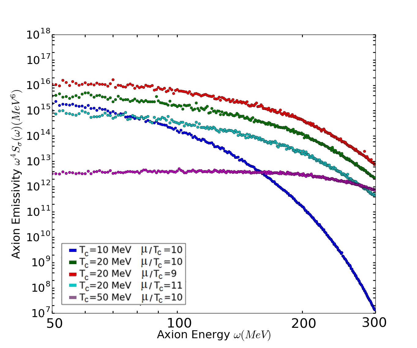
We re-evaluate $\omega$ ⁴S_$\sigma$( $\omega$ ), on which the axion emissivity depends (Eqn. 5), for T_c <20 MeV. We use the analytic simplification for the phase space integral for S_$\sigma$( $\omega$ ) from [Hannestad and Raffelt 1998] and perform a 5 dimensional numeric Monte Carlo integration as described in the Appendix A. In order to check our method we first reproduce the $\omega$ ⁴S_$\sigma$( $\omega$ ) plot from [Berenji, Gaskins, and Meyer 2016] using a T_c of 10 $-$ 50 MeV, $\mu$ /T_c = 9 $-$ 11 and p_Fn = 300 MeV (Fig. 3).

We reproduce the essential features of the [Berenji, Gaskins, and Meyer 2016] plot both in magnitude and in the following respects:

•

Increasing the value of $\mu$ /T_c for fixed T_c=20 MeV decreases amplitude of $\omega$ ⁴S_$\sigma$( $\omega$ )
•

$\omega$ ⁴S_$\sigma$( $\omega$ ) for T_c=10 MeV cuts-off at a lower value of $\omega$ =100 MeV than for T_c=20 MeV
•

The T_c=50 MeV case has lower values of $\omega$ ⁴S_$\sigma$( $\omega$ ) than the T_c=20 MeV case, with $\omega$ ⁴S_$\sigma$( $\omega$ ) remaining broadly flat across higher $\omega$ values of 100 $-$ 300 MeV with no pronounced cut-off at 200 $-$ 300 MeV
•

The value of $\omega$ ⁴S_$\sigma$( $\omega$ ) spans one order of magnitude for the 20 MeV case and varying $\mu$ /T_c = 9 $-$ 11

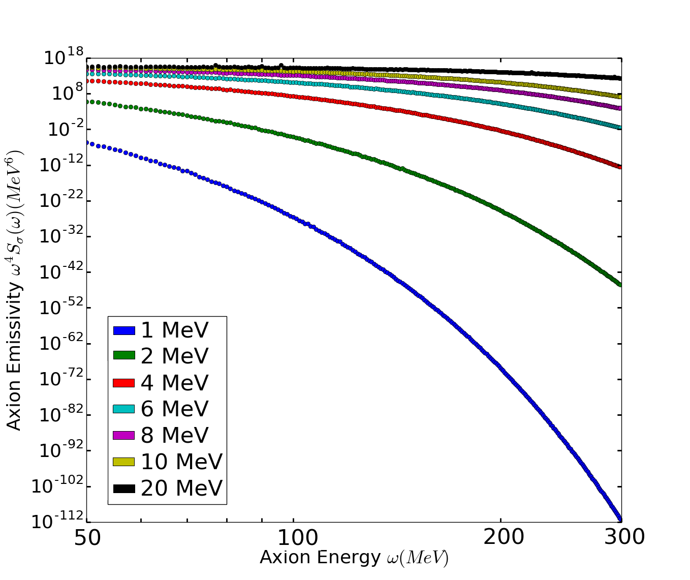
We then evaluate $\omega$ ⁴S_$\sigma$( $\omega$ ), in a lower temperature regime, for p_Fn = 300 MeV, $\mu$ /T_c = 10 and consider lower pulsar core temperatures with T_c = 1 $-$ 20 MeV (Fig. 4). Lowering T_c from 20 MeV to a plausible PNS temperature of 4 MeV reduces axion emissivity and hence gamma-ray emission by a factor of 10⁸ for axions of energy $\omega$ =100 MeV. It therefore seems implausible that there would be detectable gamma-ray emission to allow the determination of m_a using the astrophysical model of gamma-ray emission from [Berenji, Gaskins, and Meyer 2016] (Eqn. 6), for realistic pulsar core temperatures. We note however that this model is based on a quite conservative assumption that gamma-ray emission arises solely from axion radiative decay as opposed to axion to gamma-ray photon conversion in the B field of the pulsar. It is therefore possible that an alternative model allowing axion to photon conversion could produce detectable gamma-ray emission.

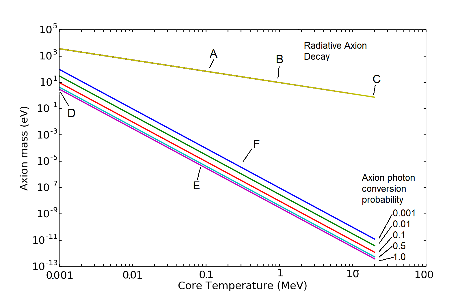
The probable lack of detectable gamma-ray emission in the lower temperature regime leads us to derive values for UL m_a from an alternative model (Eqn. 11) based on the axion power equation which defines an energy loss rate due to axion production in the pulsar core (Eqn. 9). Using the UL gamma-ray luminosity (Table 2) we determine UL m_a from Eqn. 11 whilst varying T_c and the probability of axion to photon conversion in the pulsar B field. On Fig. 5 we show the range of UL m_a values that we obtain. We see that the conversion of axions to gamma-ray photons via radiative decay results in the highest UL m_a (67.5 eV at 0.1 MeV, 9.4 eV at 1 MeV and 0.7 eV at 20 MeV, points A, B and C respectively) which is above the classic m_a search range of 10^-2 $-$ 10^-6 eV. Similarly by varying the axion to photon conversion probability from 0.001 to 1.0 (total conversion), we only obtain an UL m_a above the lower search bound of 10^-6 eV for T_c <0.1 MeV independent of the degree of axion to photon conversion or T_c <0.4 MeV assuming a probability of $\leq$ 0.001 for axion to photon conversion (Points E and F of Fig. 5 respectively). At T_c=1 keV the lowest UL m_a obtainable would be 3.0 eV assuming total conversion of axions to photons (Point D of Fig. 5). We do not offer a view on the degree of axion to photon conversion in the pulsar B field but simply present a range of conversion alternatives to give indicative values of the UL m_a.

The determination of a plausible and precise UL m_a from this alternative model thus requires both realistic lower values of T_c and a knowledge of the precise extent of the axion to photon conversion in the pulsar B field. We have dealt with the value of T_c in the PNS and old pulsar cases above; however, whilst [Berenji, Gaskins, and Meyer 2016] consider there to be no axion to photon conversion in the pulsar B field (using vacuum bi-refringence arguments) there is no consensus on the extent of axion to gamma-ray photon conversion in pulsar B fields. More attention has been paid to axion to X-ray photon inter-conversion in pulsars [Perna et al. 2012] and in axion like particle (ALP) to X-ray conversion in the higher B field (20 $\times$ 10¹⁴ G) of magnetars by [Fortin and Sinha 2018]. [Fortin and Sinha 2018] finds P_{$a\rightarrow\gamma$}=0.225 for $\omega$ = 3 keV (the peak emission) and P_{$a\rightarrow\gamma$} = 0.025 for $\omega$ = 200 keV when T_c=50 $-$ 250 keV. The lower B field of our sample notwithstanding (average $B$ =2.78 $\times$ 10¹² G) such values of P_{$a\rightarrow\gamma$} and T_c could yield constraints on m_a in the classic axion search range using the alternative model (Fig. 5).

Finally, the normalized axion energy spectrum dN_a/d $\omega$ peaks at $\omega$ /T_c = 2 [G. Raffelt 1996]. This implies that the photon energy spectrum would peak at energy T_c. Therefore for the values of T_c discussed above, in the 1 MeV range or below, the determination of an UL for unpulsed gamma-ray emission in our pulsar sample or preferably younger pulsars with a potentially higher T_c, by future low-energy gamma-ray observatories such as the All-Sky Medium Energy Gamma-ray observatory (AMEGO) or e-ASTROGAM, with greater sensitivity then any current observatory in the 0.2 $-$ 10 MeV band [Rando 2017, Angelis et al. 2018] may allow an improved determination on the UL m_a presented in this work.

Pulsar	UL Photon Flux (60-200 MeV)	UL Photon Flux (60-500 MeV)	UL m_a $\omega$ =100 MeV	UL m_a $\omega$ =200 MeV
	(From [Berenji, Gaskins, and Meyer 2016])	This analysis	(10^-2 eV)	(10^-2 eV)
	(10^-9 cm^-2 s^-1)	(10^-9 cm^-2 s^-1)
J0108-1431	4.03	1.75	0.69	2.31
J0953+0755	7.40	4.75	0.97	3.26
J0630-2834	4.82	18.90	0.97	3.25
J1136+1551	8.52	5.01	1.25	4.17

Table 5: The UL photon flux for 4 pulsars from [Berenji, Gaskins, and Meyer 2016] (60-200 MeV) compared to our analysis (60-500 MeV) and UL m_a which we derive from [Berenji, Gaskins, and Meyer 2016] fluxes for axions of energy 100 MeV and 200 MeV using Eqn. 8.

VII Conclusions

We analyze data from 17 nearby pulsars using 9 years of Fermi-LAT data and detect none. Using the UL photon flux and the astrophysical model of [Berenji, Gaskins, and Meyer 2016] which assumes a pulsar core temperature of 20 MeV we determine an improved UL axion mass (m_a) of 0.96 and 3.21 $\times$ 10^-2 eV for axions of energy 100 MeV and 200 MeV respectively. However, we show that at realistic pulsar core temperatures of <4 MeV, axion emissivity is so reduced that is unlikely a reasonable determination of UL m_a can be made with this method. An alternative axion energy loss rate model yields a plausible range of UL m_a values assuming low pulsar core temperatures but requires both the core temperature and the axion to photon conversion probability to be known to set a useful limit. Observation of the un-pulsed gamma-ray emission of our selected pulsar sample with future medium energy gamma-ray observatories such as AMEGO and e-ASTROGAM may allow a better determination of UL m_a.

Acknowledgements

We acknowledge the excellent data and analysis tools provided by the Fermi-LAT collaboration. AMB and PMC acknowledge the financial support of the UK Science and Technology Facilities Council consolidated grant ST/P000541/1. This research has made use of the SIMBAD database, operated at CDS, Strasbourg, France (Wenger et al. 2000). Finally we thank the anonymous referee for their review and very useful comments which improved this paper.

Appendix A NUCLEON PHASE SPACE INTEGRATION

The spin structure function of Eqn. 2 has an analytic simplification as presented by [Hannestad and Raffelt 1998] of which we repeat the relevant points here. From the original 12-dimensional integral, 7 dimensions may be integrated out analytically so that a 5-dimensional integral remains to be solved through numerical integration (as opposed to numerical integration of the 4-dimensional integral of [Hannestad and Raffelt 1998]).

Firstly the 3-dimensional momentum delta function is used to integrate out $d^{3}\bm{p_{4}}$ . Then, the non-relativistic nucleons have energy $E_{i}=p_{i}^{2}/2M_{N}$ and so the energy balance term c

\displaystyle E_{1}+E_{2}-E_{3}-E_{4}+\omega

\displaystyle=\frac{-2p_{3}^{2}-2\mathbf{p_{1}}\cdot\mathbf{p_{2}}+2\mathbf{p_{1}}\cdot\mathbf{p_{3}}+2\mathbf{p_{2}}\cdot\mathbf{p_{3}}}{2M_{N}}+\omega

(14)

Next, a polar co-ordinate system is used with $\alpha$ and $\beta$ being the polar and azimuthmal angles of $\bm{p_{2}}$ relative to $\bm{p_{1}}$ and $\theta$ and $\Phi$ those of $\bm{p_{3}}$ . The medium is isotropic so the $\bm{p_{1}}$ momentum can be chosen in the $z$ direction so $\int d^{3}\bm{p_{1}}=4\pi\int dp_{1}$ with $p_{1}=|\bm{p_{1}}|$ . The medium isototropy also allows the azimuthmal angle $d\Phi$ to be trivially integrated to leave three nontrivial angular integrations with the remaining angular variables expressed as follows:

\displaystyle\mathbf{p_{1}}\cdot\mathbf{p_{2}}\>=\>p_{1}p_{2}\>cos\>\alpha

(15)

\displaystyle\mathbf{p_{1}}\cdot\mathbf{p_{3}}\>=\>p_{1}p_{3}\>cos\>\theta

(16)

\displaystyle\mathbf{p_{2}}\cdot\mathbf{p_{3}}\>=\>p_{2}p_{3}\>cos\>\alpha\>cos\>\theta+\>sin\>\alpha+\>sin\>\theta+\>cos\>\beta

(17)

The integration over $d\beta$ is carried out using the $\delta$ function with $f(\beta)\equiv E_{1}+E_{2}-E_{3}-E_{4}+\omega$ and $\beta_{1}$ being the root of $f(\beta)=0$ in the interval [0, $\pi$ ] giving:

\displaystyle\int_{0}^{2\pi}\>d\beta\>\delta[f(\beta)]\>=\>\frac{2}{|df(\beta)/d\beta|_{\beta=\beta_{1}}}\>\Theta\Big(\Big|\frac{df(\beta)}{d\beta}\Big|_{\beta=\beta_{1}}^{2}\Big)

(18)

The derivative can be expressed as

\displaystyle\Big|\frac{df(\beta)}{d\beta}\Big|_{\beta=\beta_{1}}=\sqrt{az^{2}+bz+c}

(19)

where

\displaystyle z\equiv cos\>\alpha

(20)

\displaystyle a=p_{2}^{2}(-p_{1}^{2}-p_{3}^{2}+2p_{1}p_{3}cos\theta)

(21)

	$\displaystyle b=2\omega M_{N}p_{1}p_{2}-2p_{1}p_{2}p_{3}^{2}-2\omega M_{N}p_{2}p_{3}cos\theta$		(22)
	$\displaystyle+2p_{1}^{2}p_{3}cos\theta+2p_{2}p_{3}^{3}cos\theta-2p_{1}p_{2}p_{3}^{2}cos^{2}\theta$		(22)

	$\displaystyle c=\omega^{2}M_{N}^{2}+2\omega M_{N}p_{3}^{2}+p_{2}^{2}p_{3}^{2}-p_{3}^{4}-2\omega M_{N}p_{1}p_{3}cos\theta$		(23)
	$\displaystyle+2p_{1}p_{3}^{3}cos\theta-p_{1}^{2}p_{3}^{2}cos^{2}\theta-p_{2}^{2}p_{3}^{3}cos^{2}\theta$		(23)

Finally the analytic simplification of equation 18 can be solved by numerical integration through a Monte Carlo method integrating over $dp_{1}dp_{2}dp_{3}d\>cos\>\theta\>d\>cos\>\alpha$ .

References

Peccei and Quinn (1977) R. D. Pecceiand H. R. Quinn, “ $\mathrm{CP}$ conservation in the presence of pseudoparticles,” Phys. Rev. Lett. 38, 1440–1443 (1977).
Weinberg (1978) S. Weinberg, “A new light boson?” Phys. Rev. Lett. 40, 223–226 (1978).
Dine, Fischler, and Srednicki (1981) M. Dine, W. Fischler, and M. Srednicki, “A Simple Solution to the Strong CP Problem with a Harmless Axion,” Phys. Lett. 104B, 199–202 (1981).
Keil et al. (1997) W. Keil, H.-T. Janka, D. N. Schramm, G. Sigl, M. S. Turner, and J. Ellis, “Fresh look at axions and sn 1987a,” Phys. Rev. D 56, 2419–2432 (1997).
Rybka (2014) G. Rybka, “Direct detection searches for axion dark matter,” Physics of the Dark Universe 4, 14 – 16 (2014), dARK TAUP2013.
Asztalos et al. (2010) S. J. Asztalos, G. Carosi, C. Hagmann, D. Kinion, K. van Bibber, M. Hotz, L. J. Rosenberg, G. Rybka, J. Hoskins, J. Hwang, P. Sikivie, D. B. Tanner, R. Bradley, and J. Clarke, “Squid-based microwave cavity search for dark-matter axions,” Phys. Rev. Lett. 104, 041301 (2010).
Duffy et al. (2006) L. D. Duffy, P. Sikivie, D. B. Tanner, S. J. Asztalos, C. Hagmann, D. Kinion, L. J. Rosenberg, K. van Bibber, D. B. Yu, and R. F. Bradley, “High resolution search for dark-matter axions,” Phys. Rev. D 74, 012006 (2006).
Hagmann et al. (1998) C. Hagmann, D. Kinion, W. Stoeffl, K. van Bibber, E. Daw, H. Peng, L. J. Rosenberg, J. LaVeigne, P. Sikivie, N. S. Sullivan, D. B. Tanner, F. Nezrick, M. S. Turner, D. M. Moltz, J. Powell, and N. A. Golubev, “Results from a high-sensitivity search for cosmic axions,” Phys. Rev. Lett. 80, 2043–2046 (1998).
Hoskins et al. (2011) J. Hoskins, J. Hwang, C. Martin, P. Sikivie, N. S. Sullivan, D. B. Tanner, M. Hotz, L. J. Rosenberg, G. Rybka, A. Wagner, S. J. Asztalos, G. Carosi, C. Hagmann, D. Kinion, K. van Bibber, R. Bradley, and J. Clarke, “Search for nonvirialized axionic dark matter,” Phys. Rev. D 84, 121302 (2011).
Du et al. (2018) N. Du, N. Force, R. Khatiwada, E. Lentz, R. Ottens, L. J. Rosenberg, G. Rybka, G. Carosi, N. Woollett, D. Bowring, A. S. Chou, A. Sonnenschein, W. Wester, C. Boutan, N. S. Oblath, R. Bradley, E. J. Daw, A. V. Dixit, J. Clarke, S. R. O’Kelley, N. Crisosto, J. R. Gleason, S. Jois, P. Sikivie, I. Stern, N. S. Sullivan, D. B. Tanner, and G. C. Hilton (ADMX Collaboration), “Search for invisible axion dark matter with the axion dark matter experiment,” Phys. Rev. Lett. 120, 151301 (2018).
Sedrakian (2016) A. Sedrakian, “Axion cooling of neutron stars,” Phys. Rev. D 93, 065044 (2016).
Berenji, Gaskins, and Meyer (2016) B. Berenji, J. Gaskins, and M. Meyer, “Constraints on axions and axionlike particles from Fermi large area telescope observations of neutron stars,” Physical Review D 93, 13 (2016).
Iwamoto (1984) N. Iwamoto, “Axion emission from neutron stars,” Physical Review Letters 53, 1198–1201 (1984).
Iwamoto (2001) N. Iwamoto, “Nucleon-nucleon bremsstrahlung of axions and pseudoscalar particles from neutron-star matter,” Physical Review D 64, 10 (2001).
Hanhart, Phillips, and Reddy (2001) C. Hanhart, D. R. Phillips, and S. Reddy, “Neutrino and axion emissivities of neutron stars from nucleon-nucleon scattering data,” Physics Letters B 499, 9–15 (2001).
Hannestad and Raffelt (1998) S. Hannestadand G. Raffelt, “Supernova neutrino opacity from nucleon-nucleon bremsstrahlung and related processes,” Astrophysical Journal 507, 339–352 (1998).
Brinkmann and Turner (1988) R. P. Brinkmannand M. S. Turner, “Numerical rates for nucleon-nucleon, axion bremsstrahlung,” Physical Review D 38, 2338–2348 (1988).
Mayle et al. (1988) R. Mayle, J. R. Wilson, J. Ellis, K. Olive, D. N. Schramm, and G. Steigman, “Constraints on axions from sn 1987a,” Physics Letters B 203, 188 – 196 (1988).
G. Raffelt (1996) G. G. Raffelt, “Stars as laboratories for fundamental physics: The astrophysics of neutrinos, axions, and other weakly interacting particles,” Bibliovault OAI Repository, the University of Chicago Press (1996).
Raffelt (2008) G. G. Raffelt, “Astrophysical axion bounds,” Axions: Theory, Cosmology, and Experimental Searches 741, 51–71 (2008).
Manchester et al. (2005) R. N. Manchester, G. B. Hobbs, A. Teoh, and M. Hobbs, “The Australia Telescope National Facility Pulsar Catalogue,” The Astronomical Journal 129, 1993–2006 (2005), astro-ph/0412641 .
(22) Http://www.atnf.csiro.au/research/pulsar/psrcat/.
(23) Https://confluence.slac.stanford.edu/display/GLAMCOG/
Public+List+of+LAT-Detected+Gamma-Ray+Pulsars, list last updated 19^th Oct 2018, accessed on 14^th Feb 2019.
Abdo et al. (2013) A. A. Abdo, M. Ajello, A. Allafort, L. Baldini, J. Ballet, G. Barbiellini, M. G. Baring, D. Bastieri, A. Belfiore, R. Bellazzini, B. Bhattacharyya, E. Bissaldi, E. D. Bloom, E. Bonamente, et al., “The second Fermi large area telescope catalog of gamma-ray pulsars,” Astrophysical Journal Supplement Series 208, 59 (2013).
Burke-Spolaor and Bailes (2010) S. Burke-Spolaorand M. Bailes, “The millisecond radio sky: transients from a blind single-pulse search,” Monthly Notices of the Royal Astronomical Society 402, 855–866 (2010).
Jiang et al. (2017) M. Jiang, B. Y. Cui, N. A. Schmid, M. A. McLaughlin, and Z. C. Cao, “Wavelet denoising of radio observations of rotating radio transients (rrats): Improved timing parameters for eight rrats,” Astrophysical Journal 847, 13 (2017).
Bailes et al. (1997) M. Bailes, S. Johnston, J. F. Bell, D. R. Lorimer, B. W. Stappers, R. N. Manchester, A. G. Lyne, L. Nicastro, N. Damico, and B. M. Gaensler, “Discovery of four isolated millisecond pulsars,” Astrophysical Journal 481, 386–391 (1997).
Reardon et al. (2016) D. J. Reardon, G. Hobbs, W. Coles, Y. Levin, M. J. Keith, M. Bailes, N. D. R. Bhat, S. Burke-Spolaor, S. Dai, M. Kerr, P. D. Lasky, R. N. Manchester, S. Oslowski, V. Ravi, R. M. Shannon, W. van Straten, L. Toomey, J. Wang, L. Wen, X. P. You, and X. J. Zhu, “Timing analysis for 20 millisecond pulsars in the Parkes pulsar timing array,” Monthly Notices of the Royal Astronomical Society 455, 1751–1769 (2016).
Manchester et al. (1978) R. N. Manchester, A. G. Lyne, J. H. Taylor, J. M. Durdin, M. I. Large, and A. G. Little, “2nd Molonglo pulsar survey - discovery of 155 pulsars,” Monthly Notices of the Royal Astronomical Society 185, 409–421 (1978).
Siegman, Manchester, and Durdin (1993) B. C. Siegman, R. N. Manchester, and J. M. Durdin, “Timing parameters for 59 pulsars,” Monthly Notices of the Royal Astronomical Society 262, 449–455 (1993).
Manchester et al. (1996) R. N. Manchester, A. G. Lyne, N. Damico, M. Bailes, S. Johnston, D. R. Lorimer, P. A. Harrison, L. Nicastro, and J. F. Bell, “The Parkes southern pulsar survey .1. observing and data analysis systems and initial results,” Monthly Notices of the Royal Astronomical Society 279, 1235–1250 (1996).
Hobbs et al. (2004) G. Hobbs, A. G. Lyne, M. Kramer, C. E. Martin, and C. Jordan, “Long-term timing observations of 374 pulsars,” Monthly Notices of the Royal Astronomical Society 353, 1311–1344 (2004).
Pilkington et al. (1968) J. D. Pilkington, A. Hewish, S. J. Bell, and T. W. Cole, “Observations of some further pulsed radio sources,” Nature 218, 126–+ (1968).
Tauris et al. (1994) T. M. Tauris, L. Nicastro, S. Johnston, R. N. Manchester, M. Bailes, A. G. Lyne, J. Glowacki, D. R. Lorimer, and N. Damico, “Discovery of psr j0108-1431 - the closest known neutron-star,” Astrophysical Journal 428, L53–L55 (1994).
Arzoumanian et al. (1994) Z. Arzoumanian, D. J. Nice, J. H. Taylor, and S. E. Thorsett, “Timing behavior of 96 radio pulsars,” Astrophysical Journal 422, 671–680 (1994).
Large, Vaughan, and Wielebinski (1969) M. I. Large, A. E. Vaughan, and R. Wielebinski, “Highly dispersed pulsar and 3 others,” Nature 223, 1249–+ (1969).
Craft, Lovelace, and Sutton (1968) H. Craft, R. Lovelace, and J. Sutton, “New pulsar. iau circ., 2100,” 2100 (1968).
Jacoby et al. (2009) B. A. Jacoby, M. Bailes, S. M. Ord, R. T. Edwards, and S. R. Kulkarni, “A large-area survey for radio pulsars at high Galactic latitudes,” Astrophysical Journal 699, 2009–2016 (2009).
Burgay et al. (2006) M. Burgay, B. C. Joshi, N. D’Amico, A. Possenti, A. G. Lyne, R. N. Manchester, M. A. McLaughlin, M. Kramer, F. Camilo, and P. C. C. Freire, “The Parkes high-latitude pulsar survey,” Monthly Notices of the Royal Astronomical Society 368, 283–292 (2006).
Vaughan (1969) L. M. I. . W. R. Vaughan, A. E., “Three new pulsars.” Nature 222, 963 (1969).
Cole and Pilkington (1968) T. W. Coleand J. D. Pilkington, “Search for pulsating radio sources in declination range + 44 degrees delta + 90 degrees,” Nature 219, 574–+ (1968).
Camilo, Nice, and Taylor (1996) F. Camilo, D. J. Nice, and J. H. Taylor, “A search for millisecond pulsars at Galactic latitudes -50 degrees $\textless$ b $\textless$ -20 degrees,” Astrophysical Journal 461, 812–819 (1996).
Camilo and Nice (1995) F. Camiloand D. J. Nice, “Timing parameters of 29 pulsars,” Astrophysical Journal 445, 756–761 (1995).
(44) We have repeated the same analysis using the PSF3 event class which is the best quartile direction reconstruction. This does not change the determined m_a significantly considering all 17 PSRs. We therefore retain the FRONT analysis to allow direct comparison with [\rev@citealpnumRN131].
(45) Fermipy change log version 0.12.0.
Wood et al. (2017) M. Wood, R. Caputo, E. Charles, M. Di Mauro, J. Magill, and Jeremy Perkins for the Fermi-LAT Collaboration, “Fermipy: An open-source Python package for analysis of Fermi-LAT Data,” ArXiv e-prints (2017), arXiv:1707.09551 [astro-ph.IM] .
(47) As described in the Fermi Science Support Centre link https//fermi.gsfc.nasa.gov/ssc/data/analysis/scitools/source_models.html.
Leinson (2014) L. B. Leinson, “Axion mass limit from observations of the neutron star in cassiopeia a,” Journal of Cosmology and Astroparticle Physics , 11 (2014).
Ruster et al. (2005) S. B. Ruster, V. Werth, M. Buballa, I. A. Shovkovy, and D. H. Rischke, “Phase diagram of neutral quark matter: Self-consistent treatment of quark masses,” Physical Review D 72, 13 (2005).
Shen et al. (1998) H. Shen, H. Toki, K. Oyamatsu, and K. Sumiyoshi, “Relativistic equation of state of nuclear matter for supernova and neutron star,” Nuclear Physics A 637, 435–450 (1998).
Akmal, Pandharipande, and Ravenhall (1998) A. Akmal, V. R. Pandharipande, and D. G. Ravenhall, “Equation of state of nucleon matter and neutron star structure,” Physical Review C 58, 1804–1828 (1998).
Negreiros, Dexheimer, and Schramm (2012) R. Negreiros, V. A. Dexheimer, and S. Schramm, “Quark core impact on hybrid star cooling,” Physical Review C 85, 7 (2012).
Larson and Link (1999) M. B. Larsonand B. Link, “Superfluid friction and late-time thermal evolution of neutron stars,” Astrophysical Journal 521, 271–280 (1999).
Pavlov, Stringfellow, and Cordova (1996) G. G. Pavlov, G. S. Stringfellow, and F. A. Cordova, “Hubble space telescope observations of isolated pulsars,” Astrophysical Journal 467, 370–+ (1996).
Pavlov et al. (2017) G. G. Pavlov, B. Rangelov, O. Kargaltsev, A. Reisenegger, S. Guillot, and C. Reyes, “Old but still warm: Far-uv detection of psr b0950+08,” Astrophysical Journal 850, 7 (2017).
Gudmundsson, Pethick, and Epstein (1982) E. H. Gudmundsson, C. J. Pethick, and R. I. Epstein, “Neutron star envelopes,” Astrophysical Journal 259, L19–L23 (1982).
Nomoto and Tsuruta (1987) K. Nomotoand S. Tsuruta, “Cooling of neutron-stars - effects of the finite-time scale of thermal conduction,” Astrophysical Journal 312, 711–726 (1987).
Yakovlev and Pethick (2004) D. Yakovlevand C. Pethick, “Neutron star cooling,” Annual Review of Astronomy and Astrophysics 42, 169–210 (2004).
Heinke and Ho (2010) C. O. Heinkeand W. C. G. Ho, “Direct observation of the cooling of the cassiopeia a neutron star,” Astrophysical Journal Letters 719, L167–L171 (2010).
Sumiyoshi et al. (2005) K. Sumiyoshi, S. Yamada, H. Suzuki, H. Shen, S. Chiba, and H. Toki, “Postbounce evolution of core-collapse supernovae: Long-term effects of the equation of state,” Astrophysical Journal 629, 922–932 (2005).
Pons et al. (1999) J. A. Pons, S. Reddy, M. Prakash, J. M. Lattimer, and J. A. Miralles, “Evolution of proto-neutron stars,” Astrophysical Journal 513, 780–804 (1999).
Nakazato, Suzuki, and Togashi (2018) K. Nakazato, H. Suzuki, and H. Togashi, “Heavy nuclei as thermal insulation for protoneutron stars,” Phys. Rev. C 97, 035804 (2018).
Zhu, Lu, and Wang (2018) L. G. Zhu, J. L. Lu, and L. Wang, “Effects of temperature on the structure of neutron stars at high temperature,” General Relativity and Gravitation 50, 18 (2018).
Perna et al. (2012) R. Perna, W. C. G. Ho, L. Verde, M. van Adelsberg, and R. Jimenez, “Signatures of photon-axion conversion in the thermal spectra and polarization of neutron stars,” Astrophysical Journal 748, 17 (2012).
Fortin and Sinha (2018) J. F. Fortinand K. Sinha, “Constraining axion-like-particles with hard x-ray emission from magnetars,” Journal of High Energy Physics , 22 (2018).
Rando (2017) R. Rando, “The all-sky medium energy gamma-ray observatory,” Journal of Instrumentation 12, C11024 (2017).
Angelis et al. (2018) A. D. Angelis, V. Tatischeff, I. Grenier, J. McEnery, M. Mallamaci, M. Tavani, U. Oberlack, L. Hanlon, R. Walter, A. Argan, P. V. Ballmoos, A. Bulgarelli, A. Bykov, M. Hernanz, G. Kanbach, I. Kuvvetli, M. Pearce, A. Zdziarski, J. Conrad, G. Ghisellini, A. Harding, J. Isern, M. Leising, F. Longo, G. Madejski, M. Martinez, M. Mazziotta, J. Paredes, M. Pohl, R. Rando, M. Razzano, A. Aboudan, M. Ackermann, A. Addazi, M. Ajello, C. Albertus, et al., “Science with e-astrogam: A space mission for mev–gev gamma-ray astrophysics,” Journal of High Energy Astrophysics 19, 1 – 106 (2018).
Wenger et al. (2000) M. Wenger, F. Ochsenbein, D. Egret, P. Dubois, F. Bonnarel, S. Borde, F. Genova, G. Jasniewicz, S. Laloë, S. Lesteven, and R. Monier, “The SIMBAD astronomical database. The CDS reference database for astronomical objects,” Astronomy and Astrophysics Supplement 143, 9–22 (2000), astro-ph/0002110 .