跳到论文正文
W Papers独立论文阅读器 arXiv:1908.03395 论文正文 计算阅读时间 · 0%
引用这篇论文根据当前论文元数据生成,正式投稿前建议核对。


License: arXiv.org perpetual non-exclusive license
arXiv:1908.03395v1 [math.NA] 09 Aug 2019

A posteriori error estimates for the mortar
staggered DG method

Lina Zhao11 1 Department of Mathematics, The Chinese University of Hong Kong, Hong Kong Special Administrative Region. (lzhao@math.cuhk.edu.hk)    Eric Chung22 2 Department of Mathematics, The Chinese University of Hong Kong, Hong Kong Special Administrative Region. (tschung@math.cuhk.edu.hk)

Abstract: Two residual-type error estimators for the mortar staggered discontinuous Galerkin discretizations of second order elliptic equations are developed. Both error estimators are proved to be reliable and efficient. Key to the derivation of the error estimator in potential L2L^{2} error is the duality argument. On the other hand, an auxiliary function is defined, making it capable of decomposing the energy error into conforming part and nonconforming part, which can be combined with the well-known Scott-Zhang local quasi-interpolation operator and the mortar discrete formulation yields an error estimator in energy error. Importantly, our analysis for both error estimators does not require any saturation assumptions which are often needed in the literature. Several numerical experiments are presented to confirm our proposed theories.

Keywords: Staggered grids, Discontinuous Galerkin method, Nonmatching grids, A posteriori error estimates, Adaptive mesh refinement

1 Introduction

The mortar element method is a domain decomposition method with non-overlapping subdomains [5, 6]. One distinctive feature of mortar finite element method is that the meshes on adjacent subdomains are not required to be matching with each other, which makes the method well suited for problems with complicated geometries. Local features of the solution such as corner singularities or large gradients can be resolved by finer grids in the local region. Furthermore, large scale features such as geological faults and layers in subsurface flow can be modeled with nonmatching grids. Staggered discontinuous Galerkin (SDG) methods pioneered by Chung and Engquist [13, 14] earn many desirable properties such as mass conservation, superconvergence and the flexibility to deal with general quadrilateral and polygonal meshes, and have been applied to numerous partial differential equations arising from the practical applications (cf. [15, 28, 17, 20, 16, 12, 38, 40]). To further advance the applications of SDG method, a mortar formulation is developed for SDG method [24], where different triangulations in different regions of the computational domain are exploited. In the framework proposed therein, SDG discretization is employed in each subdomain and the continuity of the solution across the subdomain interfaces is imposed through the introduction of the Lagrange multipliers. The analysis developed therein shows that optimal convergence rates in both L2L^{2} and discrete energy norms are achieved. In addition, the numerical results there illustrate that if the exact solution earns local singularities, one can only obtain optimal convergence rates in regularity, not in rate. To efficiently capture the singularities and achieve optimal approximation with minimum degrees of freedom, adaptive finite element method based on a posteriori error estimators can be utilized. Due to the nonmatching meshes across the subdomain interfaces, mortar finite element methods are favored for adaptive mesh refinement. Indeed, nonmatching grids can be used on the different subdomains of a partition, this can highly reduce the number of degrees of freedom since no further nodes must be added to avoid the nonconforming meshes on the subdomain interfaces.

A posteriori error estimators have been actively studied for mixed finite element methods and discontinuous Galerkin methods on conforming grids [7, 31, 8, 22, 1, 23, 27, 25, 33, 26, 11, 21, 9, 19, 39] since the pioneering work of Babuška and Rheinboldt [2, 3]. However, a posteriori error analysis for the discretization problems on nonmatching grids is still a largely undeveloped area. Wohlmuth introduces residual type and hierarchical type a posteriori error estimators in [36, 37] for mortar finite element methods. Wheeler and Yotov [35] propose two types of a posteriori error estimators for the mortar mixed finite element method. All these estimators are constructed with some saturation assumptions. To avoid this assumption, Bernardi and Hecht present some residual type error estimators without the presence of saturation assumptions [4]. But the mesh nodes are required to be coinciding on the interface. To extend the current framework of a posteriori error analysis developed on matching grids to nonmatching grids in a more general sense, it is important to exclude the mesh restrictions on the mortar and non-mortar sides, and avoid the saturation assumptions. Recently, some residual type a posteriori error estimators are developed based on the posteriori version of the well known Strang Lemma [34], where the aforementioned restrictions are remitted.

The purpose of this paper is to design and analyze two residual type error estimators for mortar SDG method without any saturation assumptions. We first derive a reliable and efficient error estimator for mortar SDG method in potential L2L^{2} error, where the key ingredient is the duality argument. In contrast to the general error estimators developed for conforming grids, the jump of solution across the subdomain interfaces and a mortar flux difference term are also involved. Then we propose an error estimator in energy error, where some difficulties arise due to the following aspects: First, the interface grids are nonmatching across the adjacent subdomains, defining related conforming finite element spaces on the non-matching meshes as the methodology exploited in [10] is impossible; Second, mortar SDG method is a mixed type method, applying the Galerkin orthogonality directly like those proposed in [34] is infeasible. To overcome the aforementioned difficulties, we employ the well-known Scott-Zhang local quasi-interpolation operator defined in [30], which is conforming in each subdomain avoiding constructing a conforming operator over the whole domain that is usually cumbersome. Then we define an auxiliary function s∈H01​(Ω)s\in H^{1}_{0}(\Omega), which enables us to decompose the energy error into conforming part and nonconforming part. Combing the above primary ingredients, the error estimator in energy error can be derived. Again, in addition to element residual terms, the jump of solution across the subdomain interfaces and the mortar flux difference terms are also involved, where the presence of the additional terms is due to the mortar matching condition. We emphasize that our analysis for both error estimators does not need any mesh restrictions on the mortar and non-mortar sides, and saturation assumptions are also avoided.

The rest of the paper is organized as follows. In the next section, we briefly introduce the mortar formulation of SDG method. In Section 3, two residual type error estimators are proposed, and the reliability of the proposed error estimators are proved. Then, the efficiency of the proposed error estimators are established in Section 4. Several numerical experiments are carried out in Section 5, where the performances of the two error estimators are displayed. Numerical results demonstrate that singularities can be well captured and optimal convergence rates can be achieved under the adaptive mesh refinement. Finally, some conclusions are given at the end of this paper.

2 Mortar formulation of SDG method

In this section, we briefly describe the mortar formulation of SDG method by following the framework developed in [24]. The primary ingredient is to impose the continuity of the solution across subdomain interfaces by a mortar matching condition. To begin, we consider the following second order elliptic problem in two dimensions:

−∇⋅(ρ∇u)=finΩ,u=0on∂Ω,\begin{split}-\nabla\cdot(\rho\nabla u)&=f\quad\mbox{in}\;\Omega,\\ u&=0\quad\mbox{on}\;\partial\Omega,\end{split} (2.1)

where Ω\Omega is the computational domain and f⁡(x)f(x) is a given source function. We divide the domain Ω\Omega into a set of NN non-overlapping subdomains, Ω¯=∪i=1NΩ¯i\bar{\Omega}=\cup_{i=1}^{N}\bar{\Omega}_{i}. We assume, for simplicity, that {Ωi}i=1N\{\Omega_{i}\}_{i=1}^{N} is a geometrically conforming partition of Ω\Omega. We further assume that ρ\rho is a piecewise constant function, which equals ρi\rho_{i} in Ωi\Omega_{i}. Every subdomain Ωi\Omega_{i} is equipped with a quasi-uniform triangulation 𝒯hi\mathcal{T}_{h_{i}} with mesh size hi>0h_{i}>0. The triangulations {𝒯hi}i=1N\{\mathcal{T}_{h_{i}}\}_{i=1}^{N} can be non-matching across the subdomain interface Γ=∪i,j=1NΓi​j\Gamma=\cup_{i,j=1}^{N}\Gamma_{ij}, where Γi​j(=∂Ωi∩∂Ωj)\Gamma_{ij}(=\partial\Omega_{i}\cap\partial\Omega_{j}) is the interface shared by the two subdomains Ωi\Omega_{i} and Ωj\Omega_{j}. In addition, S={(i,j):Ωi​and​Ωj​have non-empty intersection}S=\{(i,j):\Omega_{i}\,\mbox{and}\,\Omega_{j}\,\mbox{have non-empty intersection}\}. In addition, we define Γi=∂Ωi∩Γ=∂Ωi\∂Ω\Gamma_{i}=\partial\Omega_{i}\cap\Gamma=\partial\Omega_{i}\backslash\partial\Omega.

Let D⊂ℝd,d=1,2D\subset\mathbb{R}^{d},d=1,2, we adopt the standard notations for the Sobolev spaces Hs​(D)H^{s}(D) and their associated norms ∥⋅∥s,D\|\cdot\|_{s,D}, and semi-norms |⋅|s,D|\cdot|_{s,D} for s≥0s\geq 0. The space H0​(D)H^{0}(D) coincides with L2​(D)L^{2}(D), for which the norm and inner products are denoted as ∥⋅∥D\|\cdot\|_{D} and (⋅,⋅)D(\cdot,\cdot)_{D}, respectively. If D=ΩD=\Omega, the subscript Ω\Omega will be dropped unless otherwise mentioned. In the sequel, we use CC to denote a generic positive constant independent of the meshsize which can have different values at different occurrences.

Next, we define some spaces which will be utilized later

Qi=L2​(Ωi)2,Q=∏i=1NQi,M=L2​(Γ)\displaystyle Q_{i}=L^{2}(\Omega_{i})^{2},\quad Q=\prod_{i=1}^{N}Q_{i},\quad M=L^{2}(\Gamma)

and

Vi={v∈H1​(Ωi),v=0​on​∂Ωi∩∂Ω},V=∏i=1NVi.\displaystyle V_{i}=\{v\in H^{1}(\Omega_{i}),v=0\;\mbox{on}\;\partial\Omega_{i}\cap\partial\Omega\},\quad V=\prod_{i=1}^{N}V_{i}.

We rewrite (2.1) into a first order system by introducing an additional unknown 𝒛\bm{z}

𝒛=ρ∇uinΩ,−∇⋅𝒛=finΩ,u=0on∂Ω,\begin{split}\bm{z}&=\rho\nabla u\hskip 12.80365pt\mbox{in}\;\Omega,\\ -\nabla\cdot\bm{z}&=f\hskip 25.6073pt\mbox{in}\;\Omega,\\ u&=0\hskip 25.6073pt\mbox{on}\;\partial\Omega,\end{split}

which can be recast into the equivalent subdomain problem

𝒛i=ρi∇uiinΩi,−∇⋅𝒛i=finΩi,𝒛i⋅𝒏i=λion∂Ωi\∂Ω,ui=0on∂Ωi∩∂Ω,λi+λj=0for all​(i,j)∈S\begin{split}\bm{z}_{i}&=\rho_{i}\nabla u_{i}\hskip 8.5359pt\mbox{in}\;\Omega_{i},\\ -\nabla\cdot\bm{z}_{i}&=f\hskip 17.07182pt\quad\mbox{in}\;\Omega_{i},\\ \bm{z}_{i}\cdot\bm{n}_{i}&=\lambda_{i}\hskip 22.76228pt\mbox{on}\;\partial\Omega_{i}\backslash\partial\Omega,\\ u_{i}&=0\hskip 17.07182pt\quad\mbox{on}\;\partial\Omega_{i}\cap\partial\Omega,\\ \lambda_{i}+\lambda_{j}&=0\hskip 25.6073pt\mbox{for all}\;(i,j)\in S\end{split} (2.2)

with an additional condition that uiu_{i} are continuous across the subdomain interface. Let 𝒏i​j\bm{n}_{ij} be the fixed unit normal direction on Γi​j\Gamma_{ij} common to the two subdomains Ωi\Omega_{i} and Ωj\Omega_{j}. We define λ\lambda on Γ\Gamma as

λ∣Γi​j=λi​𝒏i⋅𝒏i​j=λj​𝒏j⋅𝒏i​j∀Γi​j⊂Γ.\displaystyle\lambda\mid_{\Gamma_{ij}}=\lambda_{i}\,\bm{n}_{i}\cdot\bm{n}_{ij}=\lambda_{j}\,\bm{n}_{j}\cdot\bm{n}_{ij}\quad\forall\,\Gamma_{ij}\subset\Gamma.

Multiplying the equations in (2.2) by the corresponding test functions and integration by parts, we obtain the weak formulation: find (u,𝒛,λ)∈V×Q×M(u,\bm{z},\lambda)\in V\times Q\times M such that

ρi−1​(𝒛,𝒒)Ωi=(∇u,𝒒)Ωi∀𝒒∈Qi,(𝒛,∇v)Ωi−(λ​𝒏i​j⋅𝒏i,v)Γi=(f,v)Ωi∀v∈Vi,∑i=1N(⟦u⟧,μ)Γi=0∀μ∈M,\begin{split}\rho_{i}^{-1}(\bm{z},\bm{q})_{\Omega_{i}}&=(\nabla u,\bm{q})_{\Omega_{i}}\quad\forall\bm{q}\in Q_{i},\\ (\bm{z},\nabla v)_{\Omega_{i}}-(\lambda\bm{n}_{ij}\cdot\bm{n}_{i},v\,)_{\Gamma_{i}}&=(f,v)_{\Omega_{i}}\qquad\forall v\in V_{i},\\ \sum_{i=1}^{N}(\llbracket u\rrbracket,\mu)_{\Gamma_{i}}&=0\hskip 48.36958pt\forall\mu\in M,\end{split} (2.3)

where λ​𝒏i​j⋅𝒏i=𝒛∣Ωi⋅𝒏i\lambda\,\bm{n}_{ij}\cdot\bm{n}_{i}=\bm{z}\mid_{\Omega_{i}}\cdot\bm{n}_{i}.

We can rewrite (2.3) as: find (𝒛,u,λ)∈Q×V×M(\bm{z},u,\lambda)\in Q\times V\times M such that

A⁡(𝒛,u,λ,𝒒,v,μ)=(f,v)∀(𝒒,v,μ)∈Q×V×M,\displaystyle A(\bm{z},u,\lambda;\bm{q},v,\mu)=(f,v)\quad\forall(\bm{q},v,\mu)\in Q\times V\times M,

where

A⁡(𝒛,u,λ,𝒒,v,μ)=∑i=1N(ρi−1​(𝒛,𝒒)Ωi−(∇u,𝒒)Ωi+(𝒛,∇v)Ωi−(λ,v​𝒏i⋅𝒏i​j)Γi+(u​𝒏i⋅𝒏i​j,μ)Γi).\begin{split}A(\bm{z},u,\lambda;\bm{q},v,\mu)=\sum_{i=1}^{N}\Big(\rho_{i}^{-1}(\bm{z},\bm{q})_{\Omega_{i}}-(\nabla u,\bm{q})_{\Omega_{i}}+(\bm{z},\nabla v)_{\Omega_{i}}-(\lambda,v\,\bm{n}_{i}\cdot\bm{n}_{ij})_{\Gamma_{i}}+(u\bm{n}_{i}\cdot\bm{n}_{ij},\mu)_{\Gamma_{i}}\Big).\end{split}

We then present the construction of the SDG spaces for each Ωi\Omega_{i}, and the construction follows the framework given in [24]. To this end, we first introduce some notations that will be employed later. We let ℱu,i\mathcal{F}_{u,i} be the set of edges in the initial triangulation 𝒯hi\mathcal{T}_{h_{i}} excluding the edges on the interface and ℱu,i0⊂ℱu,i\mathcal{F}_{u,i}^{0}\subset\mathcal{F}_{u,i} be the set of interior edges. For each triangle τ∈𝒯hi\tau\in\mathcal{T}_{h_{i}}, we divide it into three subtriangles by connecting an interior point to the three vertices. We note that the interior point can be chosen as the centroid of the triangle to get a good regularity of the subdivided triangulation.

We denote by 𝒯i\mathcal{T}_{i} the resulting finer triangulation and by ℱp,i\mathcal{F}_{p,i} the set of edges generated by the subdivision process. In addition, we let 𝒯=∪i=1N𝒯i\mathcal{T}=\cup_{i=1}^{N}\mathcal{T}_{i}, 𝒯h=∪i=1N𝒯hi\mathcal{T}_{h}=\cup_{i=1}^{N}\mathcal{T}_{h_{i}}, ℱp=∪i=1Nℱp,i\mathcal{F}_{p}=\cup_{i=1}^{N}\mathcal{F}_{p,i}, ℱu=∪i=1Nℱu,i\mathcal{F}_{u}=\cup_{i=1}^{N}\mathcal{F}_{u,i}, ℱu0=∪i=1Nℱu,i0\mathcal{F}_{u}^{0}=\cup_{i=1}^{N}\mathcal{F}_{u,i}^{0}, ℱ0=ℱu0∪ℱp\mathcal{F}^{0}=\mathcal{F}_{u}^{0}\cup\mathcal{F}_{p}, and ℱ=ℱu∪ℱp\mathcal{F}=\mathcal{F}_{u}\cup\mathcal{F}_{p}. We use hτh_{\tau} to denote the diameter of τ∈𝒯\tau\in\mathcal{T}, heh_{e} to denote the length of edge ee, and h=maxτ∈𝒯⁡hτh=\max_{\tau\in\mathcal{T}}h_{\tau}.

For each edge ee, we define a unit normal vector 𝒏e\bm{n}_{e} as follows: If e∈ℱ∖ℱ0e\in\mathcal{F}\setminus\mathcal{F}^{0}, then 𝒏e\bm{n}_{e} is the unit normal vector of ee pointing towards the outside of Ω\Omega. If e∈ℱ0e\in\mathcal{F}^{0}, an interior edge, we then fix 𝒏e\bm{n}_{e} as one of the two possible unit normal vectors on ee. When there is no ambiguity, we use 𝒏\bm{n} instead of 𝒏e\bm{n}_{e} to simplify the notation.

Let k≥0k\geq 0 be the order of polynomial used for the approximation and Pk​(τ)P^{k}(\tau) be the set of polynomials with degree less than or equal to kk defined on τ\tau. We define the following spaces

Qhi={𝒒:𝒒∣τ∈Pk(τ)2,τ∈𝒯iand⟦𝒒⋅𝒏⟧∣e=0,∀e∈ℱp,i}\displaystyle Q_{h_{i}}=\{\bm{q}:\bm{q}\mid_{\tau}\in P^{k}(\tau)^{2},\tau\in\mathcal{T}_{i}\;\mbox{and}\;\llbracket\bm{q}\cdot\bm{n}\rrbracket\mid_{e}=0,\;\forall e\in\mathcal{F}_{p,i}\}

and

Vhi={v:v∣τ∈Pk(τ),τ∈𝒯iand⟦v⟧∣e=0,∀e∈ℱu,i},\displaystyle V_{h_{i}}=\{v:v\mid_{\tau}\in P^{k}(\tau),\tau\in\mathcal{T}_{i}\;\mbox{and}\;\llbracket v\rrbracket\mid_{e}=0,\;\forall e\in\mathcal{F}_{u,i}\},

where the jumps ⟦𝒒⋅𝒏⟧∣e\llbracket\bm{q}\cdot\bm{n}\rrbracket\mid_{e} and ⟦v⟧∣e\llbracket v\rrbracket\mid_{e} are defined in the standard way

⟦𝒒⋅𝒏⟧∣e:=𝒒∣τ1⋅𝒏−𝒒∣τ2⋅𝒏and⟦v⟧∣e:=v∣τ1−v∣τ2.\displaystyle\llbracket\bm{q}\cdot\bm{n}\rrbracket\mid_{e}:=\bm{q}\mid_{\tau_{1}}\cdot\bm{n}-\bm{q}\mid_{\tau_{2}}\cdot\bm{n}\quad\mbox{and}\quad\llbracket v\rrbracket\mid_{e}:=v\mid_{\tau_{1}}-v\mid_{\tau_{2}}.

In the above, τ1\tau_{1} and τ2\tau_{2} are the two triangles with the common edge ee. In the above definition, we assume 𝒏\bm{n} is pointing from τ1\tau_{1} to τ2\tau_{2}. In addition, we define

Vhi0={v∈Vhi:v=0​on​∂Ω∩∂Ωi}.\displaystyle V_{h_{i}}^{0}=\{v\in V_{h_{i}}:v=0\;\mbox{on}\;\partial\Omega\cap\partial\Omega_{i}\}.

On the whole computational domain, we define Vh:=∏i=1NVhi0V_{h}:=\prod_{i=1}^{N}V_{h_{i}}^{0} and Qh:=∏i=1NQhiQ_{h}:=\prod_{i=1}^{N}Q_{h_{i}}.

Refer to caption
Figure 1: Region S⁡(ν)S(\nu) (initial triangle) and Region D⁡(e)D(e) (dotted quadrilateral): ℱu\mathcal{F}_{u} (initial edges, solid line) and ℱp\mathcal{F}_{p} (new edges, dotted line) .
Refer to caption
Figure 2: Nonmatching initial triangulation in two neighbouring subdomains

We recall that Γi​j\Gamma_{ij} is the interface between Ωi\Omega_{i} and Ωj\Omega_{j}, see Fig. 2. On Γi​j\Gamma_{ij}, we introduce two different meshes called Ti​j,iT_{ij,i} and Ti​j,jT_{ij,j}, which are respectively defined as the restrictions of 𝒯hi\mathcal{T}_{h_{i}} and 𝒯hj\mathcal{T}_{h_{j}} on Γi​j\Gamma_{ij}. Among these two meshes, we select one as non-mortar mesh and the other as mortar mesh. For the non-mortar mesh, say Ti​j,iT_{ij,i}, we introduce the space of Lagrange multipliers Mi​j=Vhi0∣Γi​jM_{ij}=V_{h_{i}}^{0}\mid_{\Gamma_{ij}}, which consists of piecewise polynomials of degree up to kk defined on Γi​j\Gamma_{ij} with respect to the mesh Ti​j,iT_{ij,i}. Also, we denote the union of all the non-mortar mesh as 𝒯Γ,h=∪i,j=1NTi​j,i\mathcal{T}^{\Gamma,h}=\cup_{i,j=1}^{N}T_{ij,i}. In addition, we define Mh:=Π(i,j)∈S​Mi​jM_{h}:=\Pi_{(i,j)\in S}M_{ij}. The space MhM_{h} is used to enforce continuity of functions in VhV_{h}. Specially, we define the following mortar SDG space for the approximation of uu

V^h={v=(v1,…,vN)∈Vh:∫Γi​j(vi−vj)ψds=0∀ψ∈Mi​j,∀Γi​j⊂Γ}.\displaystyle\widehat{V}_{h}=\{v=(v_{1},\ldots,v_{N})\in V_{h}:\int_{\Gamma_{ij}}(v_{i}-v_{j})\psi\;ds=0\quad\forall\psi\in M_{ij},\;\forall\,\Gamma_{ij}\subset\Gamma\}.

Furthermore, we use S⁡(ν)S(\nu) to denote the triangle in the initial triangulation 𝒯hi\mathcal{T}_{h_{i}} with ν\nu denoting the interior point chosen in the above subdivision process. Thus, S⁡(ν)S(\nu) is the union of the three triangles in 𝒯i\mathcal{T}_{i} having the interior point ν\nu as a common vertex. For an edge e∈ℱu,i0e\in\mathcal{F}_{u,i}^{0}, we let D⁡(e)D(e) be the union of the two triangles in 𝒯i\mathcal{T}_{i} sharing the edge ee, and for an edge e∈ℱu,i∩∂Ωie\in\mathcal{F}_{u,i}\cap\partial\Omega_{i}, we let D⁡(e)D(e) be the triangle in 𝒯i\mathcal{T}_{i} having the edge ee, see Fig. 1 for an illustration. In addition for e∈𝒯Γ,he\in\mathcal{T}^{\Gamma,h}, we use D⁡(e)D(e) to denote the union of the simplicial submeshes on both sides sharing the edge ee or part of ee.

To derive the discrete version for (2.2), we introduce λh∈Mh\lambda_{h}\in M_{h} to approximate λ\lambda. We note that λh∣Γi​j\lambda_{h}\mid_{\Gamma_{ij}} is considered as an approximation of the flux 𝒛⋅𝒏i​j\bm{z}\cdot\bm{n}_{ij} on Γi​j\Gamma_{ij}. Following [24], we define

ci​(v,μ)=∑Γi​j⊂∂Ωi∫Γi​jv​μ​𝒏i⋅𝒏i​j​𝑑s∀(v,μ)∈Vhi0×∏(i,j)∈SMi​j.\displaystyle c_{i}(v,\mu)=\sum_{\Gamma_{ij}\subset\partial\Omega_{i}}\int_{\Gamma_{ij}}v\,\mu\,\bm{n}_{i}\cdot\bm{n}_{ij}\;ds\quad\forall(v,\mu)\in V_{h_{i}}^{0}\times\prod_{(i,j)\in S}M_{ij}.

We also define the following bilinear forms

bi​(𝒛,v)\displaystyle b_{i}(\bm{z},v) =(𝒛,∇v)Ωi−∑e∈ℱp,i(𝒛⋅𝒏,⟦v⟧)e,\displaystyle=(\bm{z},\nabla v)_{\Omega_{i}}-\sum_{e\in\mathcal{F}_{p,i}}(\bm{z}\cdot\bm{n},\llbracket v\rrbracket)_{e},
bi∗​(v,𝒒)\displaystyle b_{i}^{*}(v,\bm{q}) =−(v,∇⋅𝒒)Ωi+∑e∈ℱu,i0(v,⟦𝒒⋅𝒏⟧)e+(v,𝒒⋅𝒏i)Γi,\displaystyle=-(v,\nabla\cdot\bm{q})_{\Omega_{i}}+\sum_{e\in\mathcal{F}_{u,i}^{0}}(v,\llbracket\bm{q}\cdot\bm{n}\rrbracket)_{e}+(v,\bm{q}\cdot\bm{n}_{i})_{\Gamma_{i}},

where the gradient and divergence operators are elementwise operators. Integration by parts reveals that the above bilinear forms are adjoint to each other, namely, bi​(𝒒,v)=bi∗​(v,𝒒)b_{i}(\bm{q},v)=b_{i}^{*}(v,\bm{q})  ∀(v,𝒒)∈Vhi0×Qhi\forall(v,\bm{q})\in V_{h_{i}}^{0}\times Q_{h_{i}}.

With the aforementioned ingredients, the mortar SDG discretization for (2.2) reads: find (uh,𝒛h,λh)∈Vh×Qh×Mh(u_{h},\bm{z}_{h},\lambda_{h})\in V_{h}\times Q_{h}\times M_{h} such that

ρi−1​(𝒛h,𝒒)Ωi=bi∗(uh,𝒒)∀𝒒∈Qhi,i=1,…,N,bi​(𝒛h,v)−ci​(v,λh)=(f,v)Ωi∀v∈Vhi0,i=1,…,N,∑i=1Nci​(uh,μ)=0∀μ∈Mh,\begin{split}\rho_{i}^{-1}(\bm{z}_{h},\bm{q})_{\Omega_{i}}&=b_{i}^{*}(u_{h},\bm{q})\quad\;\forall\bm{q}\in Q_{h_{i}},\;i=1,\ldots,N,\\ b_{i}(\bm{z}_{h},v)-c_{i}(v,\lambda_{h})&=(f,v)_{\Omega_{i}}\qquad\forall v\in V_{h_{i}}^{0},\;i=1,\ldots,N,\\ \sum_{i=1}^{N}c_{i}(u_{h},\mu)&=0\hskip 48.36958pt\forall\mu\in M_{h},\end{split} (2.4)

which can be rewritten as: find (uh,𝒛h,λh)∈Vh×Qh×Mh(u_{h},\bm{z}_{h},\lambda_{h})\in V_{h}\times Q_{h}\times M_{h} such that

Ah​(𝒛h,uh,λh,𝒒,v,μ)=(f,v)∀(v,𝒒,μ)∈Vh×Qh×Mh,\displaystyle A_{h}(\bm{z}_{h},u_{h},\lambda_{h};\bm{q},v,\mu)=(f,v)\quad\forall(v,\bm{q},\mu)\in V_{h}\times Q_{h}\times M_{h},

where

Ah​(𝒛h,uh,λh,𝒒,v,μ)=∑i=1N(ρi−1​(𝒛,𝒒)Ωi−bi∗​(uh,𝒒)+bi​(𝒛h,v)−ci​(v,λh)+ci​(uh,μ)).\displaystyle A_{h}(\bm{z}_{h},u_{h},\lambda_{h};\bm{q},v,\mu)=\sum_{i=1}^{N}\Big(\rho_{i}^{-1}(\bm{z},\bm{q})_{\Omega_{i}}-b_{i}^{*}(u_{h},\bm{q})+b_{i}(\bm{z}_{h},v)-c_{i}(v,\lambda_{h})+c_{i}(u_{h},\mu)\Big). (2.5)

We infer from integration by parts

Ah​(𝒛−𝒛h,u−uh,λ−λh,𝒒,v,μ)=0∀(v,𝒒,μ)∈Vh×Qh×Mh.\displaystyle A_{h}(\bm{z}-\bm{z}_{h},u-u_{h},\lambda-\lambda_{h};\bm{q},v,\mu)=0\quad\forall(v,\bm{q},\mu)\in V_{h}\times Q_{h}\times M_{h}. (2.6)

We recall some a priori error estimates from [24] which are needed later to illustrate the efficiency of the proposed error estimators.

Lemma 2.1.

Let u|Ωi∈H1+σi​(Ωi)u|_{\Omega_{i}}\in H^{1+\sigma_{i}}(\Omega_{i}) with σi>1/2\sigma_{i}>1/2. Let (𝐳h,uh,λh)∈Qh×Vh×Mh(\bm{z}_{h},u_{h},\lambda_{h})\in Q_{h}\times V_{h}\times M_{h} be the solution of (2.4). Then the following estimates hold

∑i=1Nρi​‖∇(u−uh)‖0,Ωi2\displaystyle\sum_{i=1}^{N}\rho_{i}\|\nabla(u-u_{h})\|_{0,\Omega_{i}}^{2} ≤C​∑i=1Nρi​hi2​min⁡{σi,k}​‖u‖σi+1,Ωi2,\displaystyle\leq C\sum_{i=1}^{N}\rho_{i}h_{i}^{2\min\{\sigma_{i},k\}}\|u\|_{\sigma_{i}+1,\Omega_{i}}^{2},
∑i=1Nρi​‖u−uh‖0,Ωi2\displaystyle\sum_{i=1}^{N}\rho_{i}\|u-u_{h}\|_{0,\Omega_{i}}^{2} ≤C​∑i=1Nρi​hi2​min⁡{σi,k}+2​‖u‖σi+1,Ωi2,\displaystyle\leq C\sum_{i=1}^{N}\rho_{i}h_{i}^{2\min\{\sigma_{i},k\}+2}\|u\|_{\sigma_{i}+1,\Omega_{i}}^{2},
∑i=1Nρi−1​‖𝒛−𝒛h‖0,Ωi2\displaystyle\sum_{i=1}^{N}\rho_{i}^{-1}\|\bm{z}-\bm{z}_{h}\|_{0,\Omega_{i}}^{2} ≤C​∑i=1Nρi​hi2​min⁡{σi,k+12}​‖u‖σi+1,Ωi2.\displaystyle\leq C\sum_{i=1}^{N}\rho_{i}h_{i}^{2\min\{\sigma_{i},k+\frac{1}{2}\}}\|u\|_{\sigma_{i}+1,\Omega_{i}}^{2}.

3 Reliability

In this section, two residual-type error estimators are proposed. First, we develop an error estimator in potential L2L^{2} error, which mainly relies on the duality argument. Next, we propose an energy error estimator based on an auxiliary function and the well-known Scott-Zhang local quasi-interpolation operator.

3.1 Potential error estimator

To begin, we recall the following trace inequality

‖v‖0,e≤C⁡(hτ−12​‖v‖0,τ+hτ12​‖∇v‖0,τ)∀v∈H1​(τ),∀τ∈𝒯,e∈∂τ.\displaystyle\|v\|_{0,e}\leq C(h_{\tau}^{-\frac{1}{2}}\|v\|_{0,\tau}+h_{\tau}^{\frac{1}{2}}\|\nabla v\|_{0,\tau})\quad\forall v\in H^{1}(\tau),\quad\forall\tau\in\mathcal{T},\;e\in\partial\tau. (3.1)

and

‖v‖1/2,e≤C​‖v‖1,τ∀v∈H1​(τ),τ∈𝒯,e∈∂τ.\displaystyle\|v\|_{1/2,e}\leq C\|v\|_{1,\tau}\quad\forall v\in H^{1}(\tau),\tau\in\mathcal{T},e\in\partial\tau. (3.2)

We then define two interpolation operators Ii:H1​(Ωi)→VhiI_{i}:H^{1}(\Omega_{i})\rightarrow V_{h_{i}} and Ji:Hϵ​(Ωi)2→Qhi,ϵ>1/2J_{i}:H^{\epsilon}(\Omega_{i})^{2}\rightarrow Q_{h_{i}},\epsilon>1/2 by

(Ii​v,ϕ)τ\displaystyle(I_{i}v,\phi)_{\tau} =(v,ϕ)τ∀ϕ∈Pk−1​(τ),τ∈𝒯,\displaystyle=(v,\phi)_{\tau}\quad\forall\phi\in P^{k-1}(\tau),\;\tau\in\mathcal{T},
(Ii​v,ϕ)e\displaystyle(I_{i}v,\phi)_{e} =(v,ϕ)e∀ϕ∈Pk​(e),e∈ℱu\displaystyle=(v,\phi)_{e}\quad\;\forall\phi\in P^{k}(e),\;e\in\mathcal{F}_{u}

and

(Ji​𝝉,𝒒)τ\displaystyle(J_{i}\bm{\tau},\bm{q})_{\tau} =(𝝉,𝒒)τ∀𝒒∈Pk−1​(τ)2,τ∈𝒯,\displaystyle=(\bm{\tau},\bm{q})_{\tau}\qquad\;\forall\bm{q}\in P^{k-1}(\tau)^{2},\tau\in\mathcal{T},
(Ji​𝝉⋅𝒏e,ϕ)e\displaystyle(J_{i}\bm{\tau}\cdot\bm{n}_{e},\phi)_{e} =(𝝉⋅𝒏e,ϕ)e∀ϕ∈Pk​(e),e∈ℱp.\displaystyle=(\bm{\tau}\cdot\bm{n}_{e},\phi)_{e}\quad\forall\phi\in P^{k}(e),\;e\in\mathcal{F}_{p}.

In addition, we let πe\pi_{e} be the L2L^{2} projection operator onto MhM_{h}. Then, the following inequalities hold true for smooth enough functions 𝒒,v\bm{q},v and μ\mu (cf. [18, 24])

‖μ−πe​μ‖0,e≤C​he1/2​‖μ‖1/2,e,‖v−Ii​v‖0,τ≤Chτl+1∥v∥l+1,τ,l=0,1,‖v−Ii​v‖0,e≤C​he3/2​‖v‖2,τ,‖𝒒−Ji​𝒒‖0,τ≤C​hτ​‖𝒒‖1,τ,‖𝒒−Ji​𝒒‖0,e≤C​hτ1/2​‖𝒒‖1,τ.\begin{split}\|\mu-\pi_{e}\mu\|_{0,e}&\leq Ch_{e}^{1/2}\|\mu\|_{1/2,e},\\ \|v-I_{i}v\|_{0,\tau}&\leq Ch_{\tau}^{l+1}\|v\|_{l+1,\tau},\quad l=0,1,\\ \|v-I_{i}v\|_{0,e}&\leq Ch_{e}^{3/2}\|v\|_{2,\tau},\\ \|\bm{q}-J_{i}\bm{q}\|_{0,\tau}&\leq Ch_{\tau}\|\bm{q}\|_{1,\tau},\\ \|\bm{q}-J_{i}\bm{q}\|_{0,e}&\leq Ch_{\tau}^{1/2}\|\bm{q}\|_{1,\tau}.\end{split} (3.3)

On each element τ∈𝒯\tau\in\mathcal{T}, we define the local error estimator as

ητ2\displaystyle\eta_{\tau}^{2} =hτ4​‖f+∇⋅𝒛h‖0,τ2+hτ2​‖ρ−1​𝒛h−∇uh‖0,τ2+∑e∈∂τ∩ℱu0he3​‖⟦𝒛h⋅𝒏⟧‖0,e2\displaystyle=h_{\tau}^{4}\|f+\nabla\cdot\bm{z}_{h}\|_{0,\tau}^{2}+h_{\tau}^{2}\|\rho^{-1}\bm{z}_{h}-\nabla u_{h}\|_{0,\tau}^{2}+\sum_{e\in\partial\tau\cap\mathcal{F}_{u}^{0}}h_{e}^{3}\|\llbracket\bm{z}_{h}\cdot\bm{n}\rrbracket\|_{0,e}^{2}
+∑e∈∂τ∩Γhe3∥λh𝒏i⋅𝒏i​j−𝒛h⋅𝒏i∥0,e2+∑e∈∂τ∩(𝒯Γ,h∪ℱp)he∥⟦uh⟧∥0,e2.\displaystyle\;+\sum_{e\in\partial\tau\cap\Gamma}h_{e}^{3}\|\lambda_{h}\bm{n}_{i}\cdot\bm{n}_{ij}-\bm{z}_{h}\cdot\bm{n}_{i}\|_{0,e}^{2}+\sum_{e\in\partial\tau\cap(\mathcal{T}^{\Gamma,h}\cup\mathcal{F}_{p})}h_{e}\|\llbracket u_{h}\rrbracket\|_{0,e}^{2}.

Then the global error estimator in potential L2L^{2} error can be defined as

η12=∑τ∈𝒯ητ2.\displaystyle\eta_{1}^{2}=\sum_{\tau\in\mathcal{T}}\eta_{\tau}^{2}. (3.4)

The main result of this section can be stated in the next theorem.

Theorem 3.1.

Let (𝐳,u)(\bm{z},u) be the weak solution of (2.3) and (𝐳h,uh,λh)∈Qh×Vh×Mh(\bm{z}_{h},u_{h},\lambda_{h})\in Q_{h}\times V_{h}\times M_{h} be the solution of (2.4). Let η1\eta_{1} be defined in (3.4), then there exists a positive constant CC such that

‖u−uh‖0≤C​η1.\displaystyle\|u-u_{h}\|_{0}\leq C\eta_{1}.
Proof.

Assume the auxiliary problem

−∇⋅(ρ∇w)=u−uhinΩ,w=0on∂Ω\begin{split}-\nabla\cdot(\rho\nabla w)&=u-u_{h}\quad\mbox{in}\;\Omega,\\ w&=0\hskip 34.14322pt\mbox{on}\;\partial\Omega\end{split} (3.5)

satisfies the elliptic regularity estimate

‖w‖2≤C​‖u−uh‖0.\displaystyle\|w\|_{2}\leq C\|u-u_{h}\|_{0}. (3.6)

Let 𝑼=−ρ∇w\bm{U}=-\rho\nabla w and 𝑼i⋅𝒏i=μi\bm{U}_{i}\cdot\bm{n}_{i}=\mu_{i} on ∂Ωi∖∂Ω\partial\Omega_{i}\setminus\partial\Omega, then (3.5) can be recast into the following first order system

𝑼\displaystyle\bm{U} =−ρ∇winΩ,\displaystyle=-\rho\nabla w\quad\mbox{in}\;\Omega,
∇⋅𝑼\displaystyle\nabla\cdot\bm{U} =u−uhinΩ,\displaystyle=u-u_{h}\quad\mbox{in}\;\Omega,
w\displaystyle w =0on∂Ω.\displaystyle=0\hskip 34.14322pt\mbox{on}\;\partial\Omega.

Notice that the above problem is equivalent to the following subdomain problems

𝑼i=−ρi∇wiinΩi,∇⋅𝑼i=u−uhinΩi,𝑼i⋅𝒏i=μion∂Ωi\∂Ω,wi=0on∂Ωi∩∂Ω,μi+μj=0for all (i,j)∈S,\begin{split}\bm{U}_{i}&=-\rho_{i}\nabla w_{i}\;\;\mbox{in}\;\Omega_{i},\\ \nabla\cdot\bm{U}_{i}&=u-u_{h}\quad\;\mbox{in}\;\Omega_{i},\\ \bm{U}_{i}\cdot\bm{n}_{i}&=\mu_{i}\hskip 31.2982pt\mbox{on}\;\partial\Omega_{i}\backslash\partial\Omega,\\ w_{i}&=0\hskip 36.98866pt\mbox{on}\;\partial\Omega_{i}\cap\partial\Omega,\\ \mu_{i}+\mu_{j}&=0\hskip 36.98866pt\mbox{for all }\;(i,j)\in S,\end{split} (3.7)

with the additional condition that wiw_{i} are continuous across the subdomain interfaces.

Multiplying the first equation of (3.7) by 𝒛−𝒛h\bm{z}-\bm{z}_{h}, the second equation by u−uhu-u_{h} and integrating over Ω\Omega to get

‖u−uh‖02\displaystyle\|u-u_{h}\|_{0}^{2} =∑i=1N((∇⋅𝑼,u−uh)Ωi+ρi−1​(𝑼,𝒛−𝒛h)Ωi+(∇w,𝒛−𝒛h)ΩiCLOSE\displaystyle=\sum_{i=1}^{N}\Big((\nabla\cdot\bm{U},u-u_{h})_{\Omega_{i}}+\rho_{i}^{-1}(\bm{U},\bm{z}-\bm{z}_{h})_{\Omega_{i}}+(\nabla w,\bm{z}-\bm{z}_{h})_{\Omega_{i}}
OPEN−(w,(λ−λh)​𝒏i⋅𝒏i​j)Γi).\displaystyle\;-(w,(\lambda-\lambda_{h})\bm{n}_{i}\cdot\bm{n}_{ij})_{\Gamma_{i}}\Big).

Integration by parts, employing the definition of AhA_{h} (cf. (2.5)) and using 𝑼i⋅𝒏i=μi\bm{U}_{i}\cdot\bm{n}_{i}=\mu_{i} on ∂Ωi\∂Ω\partial\Omega_{i}\backslash\partial\Omega yield

‖u−uh‖02\displaystyle\|u-u_{h}\|_{0}^{2} =∑i=1N((𝑼⋅𝒏i,u−uh)Γi−∑e∈ℱp,i(𝑼⋅𝒏,⟦uh⟧)e−(𝑼,∇(u−uh))Ωi+ρi−1​(𝑼,𝒛−𝒛h)ΩiCLOSE\displaystyle=\sum_{i=1}^{N}\Big((\bm{U}\cdot\bm{n}_{i},u-u_{h})_{\Gamma_{i}}-\sum_{e\in\mathcal{F}_{p,i}}(\bm{U}\cdot\bm{n},\llbracket u_{h}\rrbracket)_{e}-(\bm{U},\nabla(u-u_{h}))_{\Omega_{i}}+\rho_{i}^{-1}(\bm{U},\bm{z}-\bm{z}_{h})_{\Omega_{i}}
OPEN+(∇w,𝒛−𝒛h)Ωi−(w,(λ−λh)​𝒏i⋅𝒏i​j)Γi)\displaystyle\;+(\nabla w,\bm{z}-\bm{z}_{h})_{\Omega_{i}}-(w,(\lambda-\lambda_{h})\bm{n}_{i}\cdot\bm{n}_{ij})_{\Gamma_{i}}\Big)
=Ah​(𝒛,u,λ,𝑼,w,μ)−Ah​(𝒛h,uh,λh,𝑼,w,μ)\displaystyle=A_{h}(\bm{z},u,\lambda;\bm{U},w,\mu)-A_{h}(\bm{z}_{h},u_{h},\lambda_{h};\bm{U},w,\mu)
=Ah​(𝒛−𝒛h,u−uh,λ−λh,𝑼,w,μ).\displaystyle=A_{h}(\bm{z}-\bm{z}_{h},u-u_{h},\lambda-\lambda_{h};\bm{U},w,\mu).

Employing (2.5) and (2.6), we deduce that

‖u−uh‖02\displaystyle\|u-u_{h}\|_{0}^{2} =Ah​(𝒛−𝒛h,u−uh,λ−λh,𝑼−Ji​𝑼,w−Ii​w,μ−πe​μ)\displaystyle=A_{h}(\bm{z}-\bm{z}_{h},u-u_{h},\lambda-\lambda_{h};\bm{U}-J_{i}\bm{U},w-I_{i}w,\mu-\pi_{e}\mu)
=∑τ∈𝒯((f+∇⋅𝒛h,w−Ii​w)τ−(ρ−1​𝒛h−∇uh,𝑼−Ji​𝑼)τCLOSE\displaystyle=\sum_{\tau\in\mathcal{T}}\Big((f+\nabla\cdot\bm{z}_{h},w-I_{i}w)_{\tau}-(\rho^{-1}\bm{z}_{h}-\nabla u_{h},\bm{U}-J_{i}\bm{U})_{\tau}
−∑e∈ℱp(⟦uh⟧,(𝑼−Ji𝑼)⋅𝒏)e−∑e∈ℱu0(⟦𝒛h⋅𝒏⟧,w−Iiw)e\displaystyle\;-\sum_{e\in\mathcal{F}_{p}}(\llbracket u_{h}\rrbracket,(\bm{U}-J_{i}\bm{U})\cdot\bm{n})_{e}-\sum_{e\in\mathcal{F}_{u}^{0}}(\llbracket\bm{z}_{h}\cdot\bm{n}\rrbracket,w-I_{i}w)_{e}
+∑i=1N((λh𝒏i⋅𝒏i​j−𝒛h⋅𝒏i,w−Iiw)Γi−(uh𝒏i⋅𝒏i​j,μ−πeμ)Γi).\displaystyle\;+\sum_{i=1}^{N}\Big((\lambda_{h}\bm{n}_{i}\cdot\bm{n}_{ij}-\bm{z}_{h}\cdot\bm{n}_{i},w-I_{i}w)_{\Gamma_{i}}-(u_{h}\bm{n}_{i}\cdot\bm{n}_{ij},\mu-\pi_{e}\mu)_{\Gamma_{i}}\Big).

The Cauchy-Schwarz inequality and the approximation properties (3.3) imply

‖u−uh‖02\displaystyle\|u-u_{h}\|_{0}^{2} ≤C⁡(∑τ∈𝒯(hτ2​‖f+∇⋅𝒛h‖0,τ​‖w‖2,τ+hτ​‖ρ−1​𝒛h−∇uh‖0,τ​‖𝑼‖1,τCLOSECLOSE\displaystyle\leq C\Big(\sum_{\tau\in\mathcal{T}}(h_{\tau}^{2}\|f+\nabla\cdot\bm{z}_{h}\|_{0,\tau}\|w\|_{2,\tau}+h_{\tau}\|\rho^{-1}\bm{z}_{h}-\nabla u_{h}\|_{0,\tau}\|\bm{U}\|_{1,\tau}
OPEN+‖λh​𝒏i⋅𝒏i​j−𝒛h⋅𝒏i‖0,∂τ∩Γ​he3/2​‖w‖2,τ)+∑e∈ℱphe1/2​‖⟦uh⟧‖0,e​‖𝑼‖1,D⁡(e)\displaystyle\;+\|\lambda_{h}\bm{n}_{i}\cdot\bm{n}_{ij}-\bm{z}_{h}\cdot\bm{n}_{i}\|_{0,\partial\tau\cap\Gamma}h_{e}^{3/2}\|w\|_{2,\tau})+\sum_{e\in\mathcal{F}_{p}}h_{e}^{1/2}\|\llbracket u_{h}\rrbracket\|_{0,e}\|\bm{U}\|_{1,D(e)}
+∑e∈ℱu0he3/2∥⟦𝒛h⋅𝒏⟧∥0,e∥w∥2,D⁡(e)+∑e∈𝒯Γ,hhe1/2∥⟦uh⟧∥0,e∥μ∥1/2,e).\displaystyle\;+\sum_{e\in\mathcal{F}_{u}^{0}}h_{e}^{3/2}\|\llbracket\bm{z}_{h}\cdot\bm{n}\rrbracket\|_{0,e}\|w\|_{2,D(e)}+\sum_{e\in\mathcal{T}^{\Gamma,h}}h_{e}^{1/2}\|\llbracket u_{h}\rrbracket\|_{0,e}\|\mu\|_{1/2,e}\Big).

This together with (3.2) and the elliptic regularity estimate (3.6) completes the proof.

∎

3.2 Energy error estimator

This section is devoted to the construction of the error estimator in energy error, the primary ingredient is to define an auxiliary function which enables us to decompose the error into conforming part and nonconforming part. To this end, we first introduce the following lemma, which provides the upper bound for the nonconforming error.

Following Lemma 3.6 of [34] and Theorem 2.2 of [22], we have

Lemma 3.1.

There exists a positive constant CC independent of the mesh size such that

minv∈H01​(Ω)∥ρ12∇(v−uh)∥0≤C(∑ℱp∪𝒯Γ,hhe−1∥⟦ρ12uh⟧∥0,e2)1/2.\displaystyle\min_{v\in H^{1}_{0}(\Omega)}\|\rho^{\frac{1}{2}}\nabla(v-u_{h})\|_{0}\leq C\Big(\sum_{\mathcal{F}_{p}\cup\mathcal{T}^{\Gamma,h}}h_{e}^{-1}\|\llbracket\rho^{\frac{1}{2}}u_{h}\rrbracket\|_{0,e}^{2}\Big)^{1/2}.

Let Πh:H1​(Ωi)→Xh​(Ωi)\Pi_{h}:H^{1}(\Omega_{i})\rightarrow X_{h}(\Omega_{i}) be the well-known Scott-Zhang local quasi-interpolation operator, where Xh​(Ωi)X_{h}(\Omega_{i}) is P1P^{1} conforming element space in each subdomain Ωi\Omega_{i}. In addition, Πh\Pi_{h} satisfies the following interpolation error estimates (cf. [30]).

Lemma 3.2.

We have the following interpolation error estimates for v∈H01​(Ω)v\in H^{1}_{0}(\Omega)

hτ−2​‖v−Πh​v‖0,τ2\displaystyle h_{\tau}^{-2}\|v-\Pi_{h}v\|_{0,\tau}^{2} ≤C​|v|1,ωττ∈𝒯i,\displaystyle\leq C|v|_{1,\omega_{\tau}}\quad\tau\in\mathcal{T}_{i},
he−1​‖v−Πh​v‖0,e2\displaystyle h_{e}^{-1}\|v-\Pi_{h}v\|_{0,e}^{2} ≤C​|v|1,ωe2e∈ℱu,i∪ℰh​(Ω¯i),\displaystyle\leq C|v|_{1,\omega_{e}}^{2}\quad e\in\mathcal{F}_{u,i}\cup\mathcal{E}_{h}(\bar{\Omega}_{i}),

where ℰh​(Ω¯i)\mathcal{E}_{h}(\bar{\Omega}_{i}) denotes all the edges of 𝒯i\mathcal{T}_{i} in Ω¯i\bar{\Omega}_{i}, and ωτ,ωe\omega_{\tau},\omega_{e} denotes the union of all the elements in 𝒯i\mathcal{T}_{i} sharing at least a node with τ\tau and ee, respectively.

We define the local error estimator on each element τ∈𝒯\tau\in\mathcal{T} as

η¯τ2=hτ2ρ−1∥f+∇⋅𝒛h∥0,τ2+∑e∈∂τ∩ℱuheρ−1∥⟦𝒛h⋅𝒏⟧∥0,e2+∥ρ−12𝒛h−ρ12∇uh∥0,τ2+∑e∈∂τ∩Γheρ−1∥λh𝒏i⋅𝒏i​j−𝒛h⋅𝒏i∥0,e2+∑e∈∂τ∩(𝒯Γ,h∪ℱp)he−1ρ∥⟦uh⟧∥0,e2.\begin{split}\bar{\eta}_{\tau}^{2}&=h_{\tau}^{2}\rho^{-1}\|f+\nabla\cdot\bm{z}_{h}\|_{0,\tau}^{2}+\sum_{e\in\partial\tau\cap\mathcal{F}_{u}}h_{e}\rho^{-1}\|\llbracket\bm{z}_{h}\cdot\bm{n}\rrbracket\|_{0,e}^{2}+\|\rho^{-\frac{1}{2}}\bm{z}_{h}-\rho^{\frac{1}{2}}\nabla u_{h}\|_{0,\tau}^{2}\\ &\;+\sum_{e\in\partial\tau\cap\Gamma}h_{e}\rho^{-1}\|\lambda_{h}\bm{n}_{i}\cdot\bm{n}_{ij}-\bm{z}_{h}\cdot\bm{n}_{i}\|_{0,e}^{2}+\sum_{e\in\partial\tau\cap(\mathcal{T}^{\Gamma,h}\cup\mathcal{F}_{p})}h_{e}^{-1}\rho\|\llbracket u_{h}\rrbracket\|_{0,e}^{2}.\end{split} (3.8)

Then, the global error estimator in energy error can be defined as

η22=∑τ∈𝒯η¯τ2.\displaystyle\eta_{2}^{2}=\sum_{\tau\in\mathcal{T}}\bar{\eta}_{\tau}^{2}. (3.9)
Theorem 3.2.

There exists a positive constant CC such that the following estimate holds

∥ρ12∇(u−uh)∥0≤Cη2.\displaystyle\|\rho^{\frac{1}{2}}\nabla(u-u_{h})\|_{0}\leq C\eta_{2}.
Proof.

We first define a function s∈H01​(Ω)s\in H^{1}_{0}(\Omega) such that

(ρ∇s,∇v)=(ρ∇uh,∇v)∀v∈H01(Ω),\displaystyle(\rho\nabla s,\nabla v)=(\rho\nabla u_{h},\nabla v)\quad\forall v\in H^{1}_{0}(\Omega), (3.10)

where the existence and uniqueness of ss follow from Riesz representation theorem.

By taking v=u−sv=u-s in (3.10), we can get

∥ρ12∇(u−uh)∥02=∥ρ12∇(u−s)∥02+∥ρ12∇(s−uh)∥02.\displaystyle\|\rho^{\frac{1}{2}}\nabla(u-u_{h})\|_{0}^{2}=\|\rho^{\frac{1}{2}}\nabla(u-s)\|_{0}^{2}+\|\rho^{\frac{1}{2}}\nabla(s-u_{h})\|_{0}^{2}. (3.11)

We can first bound the second term by employing Lemma 3.1 yielding

∥ρ12∇(s−uh)∥0≤C(∑ℱp∪𝒯Γ,hhe−1∥⟦ρ12uh⟧∥0,e2)1/2.\displaystyle\|\rho^{\frac{1}{2}}\nabla(s-u_{h})\|_{0}\leq C\Big(\sum_{\mathcal{F}_{p}\cup\mathcal{T}^{\Gamma,h}}h_{e}^{-1}\|\llbracket\rho^{\frac{1}{2}}u_{h}\rrbracket\|_{0,e}^{2}\Big)^{1/2}. (3.12)

On the other hand, we have from the definition

∥ρ12∇(u−s)∥0\displaystyle\|\rho^{\frac{1}{2}}\nabla(u-s)\|_{0} =supψ∈H01​(Ω)(ρ∇(u−s),∇ψ)∥ρ1/2∇ψ∥0\displaystyle=\sup_{\psi\in H^{1}_{0}(\Omega)}\frac{(\rho\nabla(u-s),\nabla\psi)}{\|\rho^{1/2}\nabla\psi\|_{0}}
=supψ∈H01​(Ω)(ρ∇(u−uh),∇ψ)∥ρ1/2∇ψ∥0.\displaystyle=\sup_{\psi\in H^{1}_{0}(\Omega)}\frac{(\rho\nabla(u-u_{h}),\nabla\psi)}{\|\rho^{1/2}\nabla\psi\|_{0}}.

Integration by parts implies

(ρ∇(u−uh),∇ψ)=(ρ∇(u−uh),∇(ψ−Πhψ))+(ρ∇(u−uh),∇Πhψ)=∑i=1N(ρ∇u⋅𝒏,ψ−Πhψ)Γi−(ρΔu,ψ−Πhψ)−(𝒛h,∇(ψ−Πhψ))+(ρ−12𝒛h−ρ12∇uh,ρ12∇(ψ−Πhψ))+(ρ∇(u−uh),∇Πhψ).\begin{split}(\rho\nabla(u-u_{h}),\nabla\psi)&=(\rho\nabla(u-u_{h}),\nabla(\psi-\Pi_{h}\psi))+(\rho\nabla(u-u_{h}),\nabla\Pi_{h}\psi)\\ &=\sum_{i=1}^{N}(\rho\nabla u\cdot\bm{n},\psi-\Pi_{h}\psi)_{\Gamma_{i}}-(\rho\Delta u,\psi-\Pi_{h}\psi)-(\bm{z}_{h},\nabla(\psi-\Pi_{h}\psi))\\ &\;+(\rho^{-\frac{1}{2}}\bm{z}_{h}-\rho^{\frac{1}{2}}\nabla u_{h},\rho^{\frac{1}{2}}\nabla(\psi-\Pi_{h}\psi))+(\rho\nabla(u-u_{h}),\nabla\Pi_{h}\psi).\end{split} (3.13)

The penultimate term of (3.13) can be estimated by integration by parts

(𝒛h,∇(ψ−Πh​ψ))\displaystyle(\bm{z}_{h},\nabla(\psi-\Pi_{h}\psi)) =∑e∈ℱu0(⟦𝒛h⋅𝒏⟧,ψ−Πh​ψ)e+∑i=1N(𝒛h⋅𝒏i,ψ−Πh​ψ)Γi−(∇⋅𝒛h,ψ−Πh​ψ).\displaystyle=\sum_{e\in\mathcal{F}_{u}^{0}}(\llbracket\bm{z}_{h}\cdot\bm{n}\rrbracket,\psi-\Pi_{h}\psi)_{e}+\sum_{i=1}^{N}(\bm{z}_{h}\cdot\bm{n}_{i},\psi-\Pi_{h}\psi)_{\Gamma_{i}}-(\nabla\cdot\bm{z}_{h},\psi-\Pi_{h}\psi).

The last term of (3.13) can be recast into the following form by exploiting integration by parts and the second equation of (2.4)

(ρ∇(u−uh),∇Πhψ)\displaystyle(\rho\nabla(u-u_{h}),\nabla\Pi_{h}\psi) =∑i=1N(ρ∇u⋅𝒏i,Πhψ)Γi−(ρΔu,Πhψ)−(ρ∇uh,∇Πhψ)\displaystyle=\sum_{i=1}^{N}(\rho\nabla u\cdot\bm{n}_{i},\Pi_{h}\psi)_{\Gamma_{i}}-(\rho\Delta u,\Pi_{h}\psi)-(\rho\nabla u_{h},\nabla\Pi_{h}\psi)
=∑i=1N(ρ∇u⋅𝒏i,Πhψ)Γi+(f,Πhψ)−(ρ∇uh,∇Πhψ)\displaystyle=\sum_{i=1}^{N}(\rho\nabla u\cdot\bm{n}_{i},\Pi_{h}\psi)_{\Gamma_{i}}+(f,\Pi_{h}\psi)-(\rho\nabla u_{h},\nabla\Pi_{h}\psi)
=∑i=1N(ρ∇u⋅𝒏i,Πhψ)Γi+∑i=1N(bi(𝒛h,Πhψ)−ci(Πhψ,λh))−(ρ∇uh,∇Πhψ)\displaystyle=\sum_{i=1}^{N}(\rho\nabla u\cdot\bm{n}_{i},\Pi_{h}\psi)_{\Gamma_{i}}+\sum_{i=1}^{N}(b_{i}(\bm{z}_{h},\Pi_{h}\psi)-c_{i}(\Pi_{h}\psi,\lambda_{h}))-(\rho\nabla u_{h},\nabla\Pi_{h}\psi)
=∑i=1N(ρ∇u⋅𝒏i,Πhψ)Γi+(ρ−12𝒛h−ρ12∇uh,ρ12∇Πhψ)\displaystyle=\sum_{i=1}^{N}(\rho\nabla u\cdot\bm{n}_{i},\Pi_{h}\psi)_{\Gamma_{i}}+(\rho^{-\frac{1}{2}}\bm{z}_{h}-\rho^{\frac{1}{2}}\nabla u_{h},\rho^{\frac{1}{2}}\nabla\Pi_{h}\psi)
+∑i=1N(λh𝒏i⋅𝒏i​j,ψ−Πhψ)Γi.\displaystyle\;+\sum_{i=1}^{N}(\lambda_{h}\bm{n}_{i}\cdot\bm{n}_{ij},\psi-\Pi_{h}\psi)_{\Gamma_{i}}.

Finally, we can obtain by combing the above equations

(ρ∇(u−uh),∇ψ)\displaystyle(\rho\nabla(u-u_{h}),\nabla\psi) =(ρ−12(f+∇⋅𝒛h),ρ12(ψ−Πhψ))+(ρ−12𝒛h−ρ12∇uh,ρ12∇ψ)\displaystyle=(\rho^{-\frac{1}{2}}(f+\nabla\cdot\bm{z}_{h}),\rho^{\frac{1}{2}}(\psi-\Pi_{h}\psi))+(\rho^{-\frac{1}{2}}\bm{z}_{h}-\rho^{\frac{1}{2}}\nabla u_{h},\rho^{\frac{1}{2}}\nabla\psi)
+∑i=1N(ρ−12(λh𝒏i⋅𝒏i​j−𝒛h⋅𝒏i),ρ12(ψ−Πhψ))Γi\displaystyle\;+\sum_{i=1}^{N}(\rho^{-\frac{1}{2}}(\lambda_{h}\bm{n}_{i}\cdot\bm{n}_{ij}-\bm{z}_{h}\cdot\bm{n}_{i}),\rho^{\frac{1}{2}}(\psi-\Pi_{h}\psi))_{\Gamma_{i}}
−∑e∈ℱu0(⟦ρ−12𝒛h⋅𝒏⟧,ρ12(ψ−Πhψ))e,\displaystyle\;-\sum_{e\in\mathcal{F}_{u}^{0}}(\llbracket\rho^{-\frac{1}{2}}\bm{z}_{h}\cdot\bm{n}\rrbracket,\rho^{\frac{1}{2}}(\psi-\Pi_{h}\psi))_{e},

which, coupling with (3.11), (3.12) and Lemma 3.2 yields the desired estimate.

∎

4 Efficiency

This section is devoted to establishing the lower bounds on the errors. To this end, we set the element bubble function for each element τ\tau as ψτ\psi_{\tau} and the edge bubble function for each edge ee as ψe\psi_{e}. The properties of the bubble functions are given in the next lemma.

Lemma 4.1.

The following inequalities hold for all functions v∈Pk​(τ)v\in P^{k}(\tau).

‖v‖0,τ≤C​‖ψτ1/2​v‖0,τ≤C​‖v‖0,τ,\displaystyle\|v\|_{0,\tau}\leq C\|\psi_{\tau}^{1/2}v\|_{0,\tau}\leq C\|v\|_{0,\tau}, (4.1)
‖∇(ψτ​v)‖0,τ≤C​hτ−1​‖v‖0,τ.\displaystyle\|\nabla(\psi_{\tau}v)\|_{0,\tau}\leq Ch_{\tau}^{-1}\|v\|_{0,\tau}. (4.2)

Moreover, there exists an extension operator PeP_{e} that extends any function defined on e∈ℱe\in\mathcal{F} to the element τ\tau and satisfies

he1/2​‖φ‖0,e≤C​‖ψe​Pe​φ‖0,τ≤C​he1/2​‖φ‖0,e∀φ∈Pk​(e).h_{e}^{1/2}\|\varphi\|_{0,e}\leq C\|\psi_{e}P_{e}\varphi\|_{0,\tau}\leq Ch_{e}^{1/2}\|\varphi\|_{0,e}\quad\forall\varphi\in P^{k}(e). (4.3)

Then, the lower bounds on the errors can be stated in the next theorem.

Theorem 4.1.

Let 𝒯h\mathcal{T}_{h} be shape regular and let fhf_{h} be the piecewise linear polynomial approximation of ff. Then, there exists a positive constant CC independent of hh such that

η12≤C⁡(‖u−uh‖02+∑τ∈𝒯hτ2​‖∇(u−uh)‖0,τ2+∑e∈𝒯Γ,hhe3​‖λ−λh‖0,e2CLOSE+∑τ∈𝒯(hτ4∥∇(𝒛−𝒛h)∥0,τ2+hτ2∥𝒛−𝒛h∥0,τ2+hτ4∥f−fh∥0,τ2))\begin{split}\eta_{1}^{2}&\leq C\Big(\|u-u_{h}\|_{0}^{2}+\sum_{\tau\in\mathcal{T}}h_{\tau}^{2}\|\nabla(u-u_{h})\|_{0,\tau}^{2}+\sum_{e\in\mathcal{T}^{\Gamma,h}}h_{e}^{3}\|\lambda-\lambda_{h}\|_{0,e}^{2}\\ &+\sum_{\tau\in\mathcal{T}}(h_{\tau}^{4}\|\nabla(\bm{z}-\bm{z}_{h})\|_{0,\tau}^{2}+h_{\tau}^{2}\|\bm{z}-\bm{z}_{h}\|_{0,\tau}^{2}+h_{\tau}^{4}\|f-f_{h}\|_{0,\tau}^{2})\Big)\end{split} (4.4)

and

η22≤C(∥ρ−12(𝒛−𝒛h)∥02+∑τ∈𝒯(hτ2∥ρ−12∇(𝒛−𝒛h)∥0,τ2+hτ2∥ρ−12(f−fh)∥0,τ2+hτ−2∥ρ12(u−uh)∥0,τ2+∥ρ12∇(u−uh)∥0,τ2)+∑e∈𝒯Γ,hhe∥ρ−12(λ−λh)∥0,e2).\begin{split}\eta_{2}^{2}&\leq C\Big(\|\rho^{-\frac{1}{2}}(\bm{z}-\bm{z}_{h})\|_{0}^{2}+\sum_{\tau\in\mathcal{T}}\Big(h_{\tau}^{2}\|\rho^{-\frac{1}{2}}\nabla(\bm{z}-\bm{z}_{h})\|_{0,\tau}^{2}+h_{\tau}^{2}\|\rho^{-\frac{1}{2}}(f-f_{h})\|_{0,\tau}^{2}\\ &\;+h_{\tau}^{-2}\|\rho^{\frac{1}{2}}(u-u_{h})\|_{0,\tau}^{2}+\|\rho^{\frac{1}{2}}\nabla(u-u_{h})\|_{0,\tau}^{2}\Big)+\sum_{e\in\mathcal{T}^{\Gamma,h}}h_{e}\|\rho^{-\frac{1}{2}}(\lambda-\lambda_{h})\|_{0,e}^{2}\Big).\end{split}

In addition, the following local bounds hold for any τ∈𝒯h\tau\in\mathcal{T}_{h},e∈∂τe\in\partial\tau and e^∈ℱp∪𝒯Γ,h\hat{e}\in\mathcal{F}_{p}\cup\mathcal{T}^{\Gamma,h}

hτ2​‖f+∇⋅𝒛h‖0,τ2+‖𝒛h−∇uh‖0,τ2\displaystyle h_{\tau}^{2}\|f+\nabla\cdot\bm{z}_{h}\|_{0,\tau}^{2}+\|\bm{z}_{h}-\nabla u_{h}\|_{0,\tau}^{2} ≤C⁡(‖𝒛−𝒛h‖0,τ2+‖∇(u−uh)‖0,τ2+hτ2​‖f−fh‖0,τ2),\displaystyle\leq C\Big(\|\bm{z}-\bm{z}_{h}\|_{0,\tau}^{2}+\|\nabla(u-u_{h})\|_{0,\tau}^{2}+h_{\tau}^{2}\|f-f_{h}\|_{0,\tau}^{2}\Big),
he1/2​‖⟦𝒛h⋅𝒏⟧‖0,e\displaystyle h_{e}^{1/2}\|\llbracket\bm{z}_{h}\cdot\bm{n}\rrbracket\|_{0,e} ≤C⁡(‖𝒛−𝒛h‖0,D⁡(e)+(∑τ∈D⁡(e)hτ2​‖f−fh‖0,τ2)1/2),\displaystyle\leq C\Big(\|\bm{z}-\bm{z}_{h}\|_{0,D(e)}+(\sum_{\tau\in D(e)}h_{\tau}^{2}\|f-f_{h}\|_{0,\tau}^{2})^{1/2}\Big),
he1/2​‖λh​𝒏i⋅𝒏i​j−𝒛h⋅𝒏i‖0,e\displaystyle h_{e}^{1/2}\|\lambda_{h}\bm{n}_{i}\cdot\bm{n}_{ij}-\bm{z}_{h}\cdot\bm{n}_{i}\|_{0,e} ≤C⁡(he1/2​‖λ−λh‖0,e+‖𝒛−𝒛h‖0,τ+hτ​‖∇(𝒛−𝒛h)‖0,τ)\displaystyle\leq C\Big(h_{e}^{1/2}\|\lambda-\lambda_{h}\|_{0,e}+\|\bm{z}-\bm{z}_{h}\|_{0,\tau}+h_{\tau}\|\nabla(\bm{z}-\bm{z}_{h})\|_{0,\tau}\Big)

and

∥⟦uh⟧∥0,e^≤C∑τ∈D⁡(e^)(hτ−1/2∥u−uh∥0,τ+hτ1/2∥∇(u−uh)∥0,τ).\displaystyle\|\llbracket u_{h}\rrbracket\|_{0,\hat{e}}\leq C\sum_{\tau\in D(\hat{e})}\Big(h_{\tau}^{-1/2}\|u-u_{h}\|_{0,\tau}+h_{\tau}^{1/2}\|\nabla(u-u_{h})\|_{0,\tau}\Big).
Proof.

Let Rτ​(f)=f+∇⋅𝒛hR_{\tau}(f)=f+\nabla\cdot\bm{z}_{h}. Green’s theorem and the Cauchy-Schwarz inequality imply

(Rτ​(fh),ψτ​Rτ​(fh))τ\displaystyle(R_{\tau}(f_{h}),\psi_{\tau}R_{\tau}(f_{h}))_{\tau} =(−∇⋅(𝒛−𝒛h),ψτRτ(fh))τ+(fh−f,ψτRτ(fh))τ\displaystyle=(-\nabla\cdot(\bm{z}-\bm{z}_{h}),\psi_{\tau}R_{\tau}(f_{h}))_{\tau}+(f_{h}-f,\psi_{\tau}R_{\tau}(f_{h}))_{\tau}
=(𝒛−𝒛h,∇(ψτ​Rτ​(fh)))τ+(fh−f,ψτ​Rτ​(fh))τ\displaystyle=(\bm{z}-\bm{z}_{h},\nabla(\psi_{\tau}R_{\tau}(f_{h})))_{\tau}+(f_{h}-f,\psi_{\tau}R_{\tau}(f_{h}))_{\tau}
≤C⁡(‖𝒛−𝒛h‖0,τ​‖∇(ψτ​Rτ​(fh))‖0,τ+‖f−fh‖0,τ​‖ψτ​Rτ​(fh)‖0,τ)\displaystyle\leq C(\|\bm{z}-\bm{z}_{h}\|_{0,\tau}\|\nabla(\psi_{\tau}R_{\tau}(f_{h}))\|_{0,\tau}+\|f-f_{h}\|_{0,\tau}\|\psi_{\tau}R_{\tau}(f_{h})\|_{0,\tau})
≤C⁡(‖𝒛−𝒛h‖0,τ​hτ−1​‖Rτ​(fh)‖0,τ+‖f−fh‖0,τ​‖Rτ​(fh)‖0,τ),\displaystyle\leq C(\|\bm{z}-\bm{z}_{h}\|_{0,\tau}h_{\tau}^{-1}\|R_{\tau}(f_{h})\|_{0,\tau}+\|f-f_{h}\|_{0,\tau}\|R_{\tau}(f_{h})\|_{0,\tau}),

where in the last inequality, we use (4.1) and (4.2).

Combining the above inequality with (4.1), we can achieve

‖Rτ​(fh)‖0,τ2≤C⁡(‖𝒛−𝒛h‖0,τ​hτ−1​‖Rτ​(fh)‖0,τ+‖f−fh‖0,τ​‖Rτ​(fh)‖0,τ),\displaystyle\|R_{\tau}(f_{h})\|_{0,\tau}^{2}\leq C(\|\bm{z}-\bm{z}_{h}\|_{0,\tau}h_{\tau}^{-1}\|R_{\tau}(f_{h})\|_{0,\tau}+\|f-f_{h}\|_{0,\tau}\|R_{\tau}(f_{h})\|_{0,\tau}),

which yields

hτ​‖Rτ​(f)‖0,τ≤C⁡(‖𝒛−𝒛h‖0,τ+hτ​‖f−fh‖0,τ).\displaystyle h_{\tau}\|R_{\tau}(f)\|_{0,\tau}\leq C(\|\bm{z}-\bm{z}_{h}\|_{0,\tau}+h_{\tau}\|f-f_{h}\|_{0,\tau}). (4.5)

Next, fix an edge e∈ℱu0e\in\mathcal{F}_{u}^{0}, for any w=ψe​Pe​⟦𝒛h⋅𝒏⟧∈H01​(D⁡(e))w=\psi_{e}P_{e}\llbracket\bm{z}_{h}\cdot\bm{n}\rrbracket\in H^{1}_{0}(D(e)), we have from integration by parts

(⟦𝒛h⟧⋅𝒏e,ψe​Pe​⟦𝒛h⋅𝒏⟧)e\displaystyle(\llbracket\bm{z}_{h}\rrbracket\cdot\bm{n}_{e},\psi_{e}P_{e}\llbracket\bm{z}_{h}\cdot\bm{n}\rrbracket)_{e} =∑τ∈D⁡(e)((𝒛h−𝒛)⋅𝒏τ,ψe​Pe​⟦𝒛h⋅𝒏⟧)∂τ\displaystyle=\sum_{\tau\in D(e)}((\bm{z}_{h}-\bm{z})\cdot\bm{n}_{\tau},\psi_{e}P_{e}\llbracket\bm{z}_{h}\cdot\bm{n}\rrbracket)_{\partial\tau}
=∑τ∈D⁡(e)((∇⋅(𝒛h−𝒛),ψe​Pe​⟦𝒛h⋅𝒏⟧)τ+(𝒛h−𝒛,∇(ψe​Pe​⟦𝒛h⋅𝒏⟧))τ)\displaystyle=\sum_{\tau\in D(e)}\Big((\nabla\cdot(\bm{z}_{h}-\bm{z}),\psi_{e}P_{e}\llbracket\bm{z}_{h}\cdot\bm{n}\rrbracket)_{\tau}+(\bm{z}_{h}-\bm{z},\nabla(\psi_{e}P_{e}\llbracket\bm{z}_{h}\cdot\bm{n}\rrbracket))_{\tau}\Big)
=∑τ∈D⁡(e)((Rτ​(f),ψe​Pe​⟦𝒛h⋅𝒏⟧)τ+(𝒛h−𝒛,∇(ψe​Pe​⟦𝒛h⋅𝒏⟧))τ),\displaystyle=\sum_{\tau\in D(e)}((R_{\tau}(f),\psi_{e}P_{e}\llbracket\bm{z}_{h}\cdot\bm{n}\rrbracket)_{\tau}+(\bm{z}_{h}-\bm{z},\nabla(\psi_{e}P_{e}\llbracket\bm{z}_{h}\cdot\bm{n}\rrbracket))_{\tau}),

which, coupling with (4.3), inverse inequality and (4.5) yields

‖⟦𝒛h⋅𝒏⟧‖0,e2≤C​∑τ∈D⁡(e)(‖𝒛−𝒛h‖0,τ​‖∇(ψe​Pe​⟦𝒛h⋅𝒏⟧)‖0,τ+‖f+∇⋅𝒛h‖0,τ​‖ψe​Pe​⟦𝒛h⋅𝒏⟧‖0,τ)≤C​∑τ∈D⁡(e)(‖𝒛−𝒛h‖0,τ​hτ−1​‖ψe​Pe​⟦𝒛h⋅𝒏⟧‖0,τ+‖f+∇⋅𝒛h‖0,τ​‖ψe​Pe​⟦𝒛h⋅𝒏⟧‖0,τ)≤C⁡((∑τ∈D⁡(e)‖𝒛−𝒛h‖0,τ2)1/2+(∑τ∈D⁡(e)hτ2​‖f−fh‖0,τ2)12)​he−12​‖⟦𝒛h⋅𝒏⟧‖0,e.\begin{split}\|\llbracket\bm{z}_{h}\cdot\bm{n}\rrbracket\|_{0,e}^{2}&\leq C\sum_{\tau\in D(e)}\Big(\|\bm{z}-\bm{z}_{h}\|_{0,\tau}\|\nabla(\psi_{e}P_{e}\llbracket\bm{z}_{h}\cdot\bm{n}\rrbracket)\|_{0,\tau}+\|f+\nabla\cdot\bm{z}_{h}\|_{0,\tau}\|\psi_{e}P_{e}\llbracket\bm{z}_{h}\cdot\bm{n}\rrbracket\|_{0,\tau}\Big)\\ &\leq C\sum_{\tau\in D(e)}\Big(\|\bm{z}-\bm{z}_{h}\|_{0,\tau}h_{\tau}^{-1}\|\psi_{e}P_{e}\llbracket\bm{z}_{h}\cdot\bm{n}\rrbracket\|_{0,\tau}+\|f+\nabla\cdot\bm{z}_{h}\|_{0,\tau}\|\psi_{e}P_{e}\llbracket\bm{z}_{h}\cdot\bm{n}\rrbracket\|_{0,\tau}\Big)\\ &\leq C\Big(\Big(\sum_{\tau\in D(e)}\|\bm{z}-\bm{z}_{h}\|_{0,\tau}^{2}\Big)^{1/2}+\Big(\sum_{\tau\in D(e)}h_{\tau}^{2}\|f-f_{h}\|_{0,\tau}^{2}\Big)^{\frac{1}{2}}\Big)h_{e}^{-\frac{1}{2}}\|\llbracket\bm{z}_{h}\cdot\bm{n}\rrbracket\|_{0,e}.\end{split}

Thus

he1/2​‖⟦𝒛h⋅𝒏⟧‖0,e≤C⁡(‖𝒛−𝒛h‖0,D⁡(e)+(∑τ∈D⁡(e)hτ2​‖f−fh‖0,τ2)1/2).\displaystyle h_{e}^{1/2}\|\llbracket\bm{z}_{h}\cdot\bm{n}\rrbracket\|_{0,e}\leq C(\|\bm{z}-\bm{z}_{h}\|_{0,D(e)}+(\sum_{\tau\in D(e)}h_{\tau}^{2}\|f-f_{h}\|_{0,\tau}^{2})^{1/2}).

Triangle inequality implies

‖𝒛h−∇uh‖0≤‖𝒛−𝒛h‖0+‖∇(u−uh)‖0.\displaystyle\|\bm{z}_{h}-\nabla u_{h}\|_{0}\leq\|\bm{z}-\bm{z}_{h}\|_{0}+\|\nabla(u-u_{h})\|_{0}.

Finally, the triangle inequality and trace inequality (3.1) yield

‖λh​𝒏i⋅𝒏i​j−𝒛h⋅𝒏i‖0,e\displaystyle\|\lambda_{h}\bm{n}_{i}\cdot\bm{n}_{ij}-\bm{z}_{h}\cdot\bm{n}_{i}\|_{0,e} ≤C⁡(‖λ−λh‖0,e+‖𝒛⋅𝒏−𝒛h⋅𝒏‖0,e)\displaystyle\leq C(\|\lambda-\lambda_{h}\|_{0,e}+\|\bm{z}\cdot\bm{n}-\bm{z}_{h}\cdot\bm{n}\|_{0,e})
≤C(∥λ−λh∥0,e+hτ−1/2∥𝒛−𝒛h∥0,τ+hτ1/2∥∇(𝒛−𝒛h)∥0,τ)\displaystyle\leq C\Big(\|\lambda-\lambda_{h}\|_{0,e}+h_{\tau}^{-1/2}\|\bm{z}-\bm{z}_{h}\|_{0,\tau}+h_{\tau}^{1/2}\|\nabla(\bm{z}-\bm{z}_{h})\|_{0,\tau}\Big)

and

∥⟦uh⟧∥0,e^=∥⟦u−uh⟧∥0,e^≤C∑τ∈D⁡(e^)(hτ−1/2∥u−uh∥0,τ+hτ1/2∥∇(u−uh)∥0,τ).\displaystyle\|\llbracket u_{h}\rrbracket\|_{0,\hat{e}}=\|\llbracket u-u_{h}\rrbracket\|_{0,\hat{e}}\leq C\sum_{\tau\in D(\hat{e})}\Big(h_{\tau}^{-1/2}\|u-u_{h}\|_{0,\tau}+h_{\tau}^{1/2}\|\nabla(u-u_{h})\|_{0,\tau}\Big).

The preceding arguments complete the assertion. ∎

Remark 4.1.

It follows from Lemma 2.1 that the orders of convergence for all the terms present in the right hand side of (4.4) are comparable to ‖u−uh‖0\|u-u_{h}\|_{0}. Thus, this bound, combined with Theorem 3.1, implies that η1\eta_{1} is an efficient and reliable estimator for the potential L2L^{2} error. Similarly, η2\eta_{2} is also an efficient and reliable estimator for the energy error.

5 Numerical experiments

In this section we present several numerical experiments to demonstrate the performance of the proposed error estimators. The adaptive mesh pattern and convergence history are reported for each example. In all of our simulations, we use piecewise linear elements, i.e., k=1k=1. Since the new triangulation 𝒯\mathcal{T} is only formed to define the method and it is not a refinement. Therefore, in our refinement algorithm, we will carry out the refinement on 𝒯h\mathcal{T}_{h} by an estimator defined on each ρ∈𝒯h\rho\in\mathcal{T}_{h}. We define the error estimator as

ξρ=∑τ∈𝒯,τ∩ρ≠∅ητ2.\displaystyle\xi_{\rho}=\sum_{\tau\in\mathcal{T},\tau\cap\rho\neq\emptyset}\eta_{\tau}^{2}.

Moreover, for any subset ℳ⊂𝒯h\mathcal{M}\subset\mathcal{T}_{h}, we define

ξ2​(ℳ):=∑ρ∈ℳξ2​(ρ).\displaystyle\xi^{2}(\mathcal{M}):=\sum_{\rho\in\mathcal{M}}\xi^{2}(\rho).

Similar definitions can be applied for η¯τ\bar{\eta}_{\tau} defined in (3.8).

Our adaptive refinement can be implemented by the following iteration:

  1. 1.

    Start with an initial mesh 𝒯h0\mathcal{T}_{h}^{0}.

  2. 2.

    Solve the discrete problem (2.4) for (𝒖hℓ,𝒛hℓ,phℓ)(\bm{u}_{h}^{\ell},\bm{z}_{h}^{\ell},p_{h}^{\ell}) with respect to 𝒯hℓ\mathcal{T}_{h}^{\ell}.

  3. 3.

    Compute ξρ,∀ρ∈𝒯hℓ\xi_{\rho},\forall\rho\in\mathcal{T}_{h}^{\ell}.

  4. 4.

    Mark the minimal set ℳ⊆𝒯h\mathcal{M}\subseteq\mathcal{T}_{h} satisfying θ​∑ρ∈𝒯hξρ2≤∑ρ∈ℳξρ2\theta\sum_{\rho\in\mathcal{T}_{h}}\xi_{\rho}^{2}\leq\sum_{\rho\in\mathcal{M}}\xi_{\rho}^{2} for some fixed parameter θ∈(0,1)\theta\in(0,1).

  5. 5.

    Refine marked triangles and compute 𝒯hℓ+1\mathcal{T}^{\ell+1}_{h} by red and green refinement for adaptive mesh. Update ℓ\ell and go to step 2.

Example 5.1.

In this example, Ω=(0,1)2\Omega=(0,1)^{2} and ρ=1\rho=1, we consider the exact solution given by

u⁡(x,y)=1000​x​y​e−100​(x2+y2).\displaystyle u(x,y)=1000xye^{-100(x^{2}+y^{2})}.

The global domain Ω\Omega is decomposed into four square subdomains and the initial grid in each subdomain is 2×22\times 2.

The contour plot of the exact solution and the adaptive mesh pattern arising from the energy error estimator are reported in Fig. 3. The adaptive mesh pattern for the error estimator in potential L2L^{2} error is similar and is omitted for simplicity. We note that the grids are appropriately refined along the boundary layers.

The convergence history for ‖u−uh‖0\|u-u_{h}\|_{0} and η1\eta_{1} as well as ‖∇(u−uh)‖0\|\nabla(u-u_{h})\|_{0} and η2\eta_{2} are displayed in Fig. 4. We observe that the adaptive solution needs much fewer elements to provide the same accuracy.

Refer to caption
Refer to caption
Figure 3: The contour plot of the exact solution and the adaptive mesh pattern for example 1.
Refer to caption
Refer to caption
Figure 4: Convergence history: potential error estimator (left) and energy error estimator (right).
Example 5.2.

In this example, we consider a non-smooth solution in H3/2−δ​(Ω)H^{3/2-\delta}(\Omega) with δ>0\delta>0 defined by u⁡(r,θ)=r1/2​cos⁡(2​θ)u(r,\theta)=r^{1/2}\cos(2\theta) with polar coordinates (r,θ)(r,\theta) centered at (0.5,0.5)(0.5,0.5). In addition, we let ρ=1\rho=1. We assume that the computational domain is decomposed into four square subdomains.

The initial mesh and adaptive mesh pattern using the energy error estimator are shown in Fig. 6. We observe that the singularly can be well captured by the proposed error estimators.

The convergence history for ‖u−uh‖0\|u-u_{h}\|_{0} and η1\eta_{1} as well as ‖∇(u−uh)‖0\|\nabla(u-u_{h})\|_{0} and η2\eta_{2} under uniform refinement and adaptive refinement, respectively, are shown in Fig. 7. It is clear that the order of convergence for ‖u−uh‖0\|u-u_{h}\|_{0} and η1\eta_{1} under uniform refinement is approximately 1.5, while the order of convergence for ‖u−uh‖0\|u-u_{h}\|_{0} and η1\eta_{1} under adaptive refinement is approximately 2. On the other hand, the order of convergence for ‖∇(u−uh)‖0\|\nabla(u-u_{h})\|_{0} and η2\eta_{2} under uniform refinement is approximately 0.5, while the order of convergence for ‖∇(u−uh)‖0\|\nabla(u-u_{h})\|_{0} and η2\eta_{2} under adaptive refinement is approximately 1. This demonstrates that under uniform refinement we can achieve the reduced convergence rate reflecting singularity, and optimal convergence rates can be recovered by employing adaptive mesh refinement. This example highlights that adaptive mesh refinement outperforms uniform mesh refinement and can lead to optimal convergence rate even with low solution regularity.

Refer to caption
Figure 5: The contour plot of the exact solution for example 2.
Refer to caption
Refer to caption
Figure 6: Initial mesh (left) and adaptive mesh pattern (right).
Refer to caption
Refer to caption
Figure 7: Convergence history: potential error estimator (left) and energy error estimator (right).
Example 5.3.

Our third example is an interface problem which exhibits an interface singularity, cf. [29, 32]. Consider Ω=(−1,1)×(−1,1)\Omega=(-1,1)\times(-1,1), divided into four subdomains Ωi\Omega_{i} along the Cartesian axes (the subregion {x>0,y>0}∩Ω\{x>0,y>0\}\cap\Omega is denoted as Ω1\Omega_{1} and the subsequent numbering is done counterclockwise). The exact solution is given by

u⁡(r,θ)=rα​(Ki​sin⁡(α​θ)+Si​cos⁡(α​θ))\displaystyle u(r,\theta)=r^{\alpha}(K_{i}\sin(\alpha\theta)+S_{i}\cos(\alpha\theta))

in each Ωi\Omega_{i}. The solution is continuous across the interfaces and the normal component of its flux 𝒛\bm{z} is continuous; it exhibits a singularity at the origin and it only belongs to H1+α​(Ω)H^{1+\alpha}(\Omega). We take the piecewise constant coefficient as ρ1=ρ3=5,ρ2=ρ4=1\rho_{1}=\rho_{3}=5,\rho_{2}=\rho_{4}=1 and α=0.53544095\alpha=0.53544095. The values of Ki,SiK_{i},S_{i} can be found in, e.g., [32].

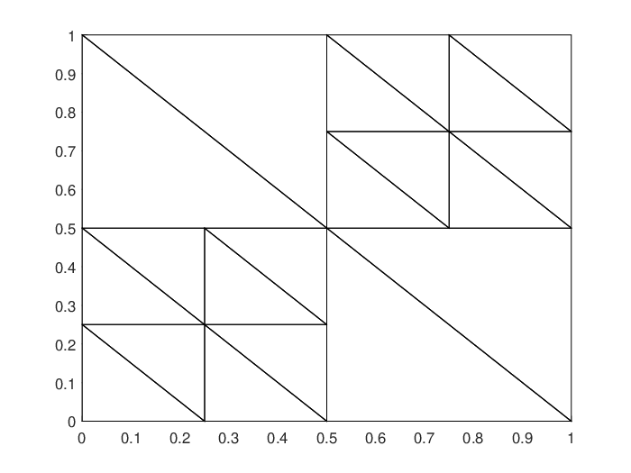
The initial mesh is the same as Fig. 7 and the convergence history and adaptive mesh pattern are reported in Fig. 8 and Fig. 9, respectively. Again, reduced convergence rate can be achieved for uniform refinement due to low solution regularity, while optimal convergence rates can be recovered by employing adaptive mesh refinement. In addition, the singularity is well captured. This example once again illustrates that the proposed error estimators can guide adaptive mesh refinement.

Refer to caption
Refer to caption
Figure 8: Convergence history: potential error estimator (left) and energy error estimator (right).
Refer to caption
Refer to caption
Figure 9: Approximate solution on adaptively refined meshes (left) and adaptive mesh pattern for energy error estimator (right).

6 Conclusion

In this paper, we have proposed two residual-type error estimators in potential L2L^{2} error and energy error, respectively. The proposed error estimators are proved to be reliable and efficient. The key idea is to exploit the duality argument for potential L2L^{2} error. To derive an error estimator in energy error, we decompose the energy error into conforming part and nonconforming part via the introduction of an auxiliary function. The numerical results demonstrate that the singularities can be well captured by the proposed error estimators, in addition, the superiority of adaptive mesh refinement over uniform mesh refinement is clearly visible in the improved convergence rate for solutions of limited regularity.

Acknowledgements

The research of Eric Chung is partially supported by the Hong Kong RGC General Research Fund (Project numbers 14304217 and 14302018), CUHK Faculty of Science Direct Grant 2018-19 and NSFC/RGC Joint Research Scheme (Project number HKUST620/15).

References

  • [1] M. Ainsworth, A posteriori error estimation for lowest order Raviart-Thomas mixed finite elements, SIAM J. Sci. Comput., 30 (2005), pp. 189–204.
  • [2] I. Babuška and W. C. Rheinboldt, Error estimates for adaptive finite element computations, SIAM J. Numer. Anal., 15 (1978), pp. 736–754.
  • [3] I. Babuška and W. C. Rheinboldt, A posteriori error estimates for the finite element method, Int. J. Numer. Methods Eng., 12 (1978), pp. 1597–1615.
  • [4] C. Bernardi and F. Hecht, Error indicators for the mortar finite element discretization of the Laplace equations, Math. Comp., 71 (2002), pp. 1371–1403.
  • [5] C. Bernardi, Y. Maday, and A. T. Patera, Domain decomposition by the mortar element method, In: H. G. Kaper, M. Garbey, G. W. Pieper, Asymptotic and Numerical Methods for Partial Differential Equations with Critical Parametera, pp. 269–286. Kluwer, Dordrect (1993).
  • [6] C. Bernardi, Y. Maday, and A. T. Patera, A new nonconforming approach to domain decomposition: the mortar element method, In: H. Brezis, J. L. Lions, Nonlinear Partial Differential Equations and their Application, College De France Seminar, vol. XI, pp. 13–51. Pitman, London (1994).
  • [7] D. Braess and R. Verfürth, A posteriori error estimators for the Raviart-Thomas element, SIAM J. Numer. Anal., 33 (1996), pp. 2431–2444.
  • [8] C. Carstensen, A posteriori error estimate for the mixed finite element method, Math. Comp., 66 (1997), pp. 465–476.
  • [9] C. Carstensen and J. Gedicke, Robust residual-based a posteriori Arnold–Winther mixed finiteelement analysis in elasticity, Comput. Methods Appl. Mech. Engrg., 300 (2016), pp. 245-264.
  • [10] C. Carstensen and J. Hu, A unifying theory of a posteriori error control for nonconforming finite element methods, Numer. Math., 107 (2007), pp. 473-502.
  • [11] C. Carstensen, D. Kim, and E.-J. Park, A priori and a posteriori pseudostress-velocity mixed finite element error analysis for the Stokes problem, SIAM J. Numer. Anal., 49 (2011), pp. 2501-2523.
  • [12] S. Cheung, E. T. Chung and H. Kim, A mass conservative scheme for fluid-structure interaction problems by the staggered discontinuous Galerkin method, J. Sci. Comput., 74 (2018), pp. 1423–1456.
  • [13] E. T. Chung and B. Engquist, Optimal discontinuous Galerkin methods for wave propagation, SIAM J. Numer. Anal., 44 (2006), pp. 2131–2158.
  • [14] E. T. Chung and B. Engquist, Optimal discontinuous Galerkin methods for the acoustic wave equation in higher dimensions, SIAM J. Numer. Anal., 47 (2009), pp. 3820–3848.
  • [15] E. T. Chung, B. Cockburn, and G. Fu, The staggered DG method is the limit of a hybridizable DG method. Part II: the Stokes flow, J. Sci. Comput., 66 (2016), pp. 870–887.
  • [16] E. T. Chung, E.-J. Park, and L. Zhao, Guaranteed a posteriori error estimates for a staggered discontinuous Galerkin method, J. Sci. Comput., 75 (2018), pp. 1079–1101.
  • [17] E. T. Chung and W. Qiu, Analysis of an SDG method for the incompressible Navier-Stokes equations, SIAM. J. Numer. Anal., 55 (2017), pp. 543–569.
  • [18] P. G. Ciarlet, The Finite Element Method for Elliptic Problems, North-Holland Publishing, Amsterdam, 1978.
  • [19] J. Du and E. T. Chung, An adaptive staggered discontinuous Galerkin method for the steady state convection-diffusion equation, J. Sci. Comput., 77 (2018), pp. 1490–1518.
  • [20] J. Du, E. T. Chung, M. Lam, and X.-P. Wang, Discontinuous Galerkin method with staggered hybridization for a class of nonlinear Stokes equations, J. Sci. Comput., 76 (2018), pp. 1547–1577.
  • [21] A. Ern and M. Vohralík, Polynomial-degree-robust a posteriori estimates in a unified setting for conforming, nonconforming, discontinuous Galerkin, and mixed discretizations, SIAM J. Numer. Anal., 53 (2015), pp. 1058–1081.
  • [22] O. A. Karakashian and F. Pascal, A posteriori error estimates for a discontinuous Galerkin approximation of second-order elliptic problems, SIAM J. Numer. Anal., 41 (2003), pp. 2374–2399.
  • [23] K. Y. Kim, A posteriori error analysis for locally conservative mixed methods, Math. Comp., 76 (2007), pp. 43–66.
  • [24] H. Kim, E. T. Chung, and C.-Y. Lam, Mortar formulation for a class of staggered discontinuous Galerkin methods, Comput. Math. Appl., 71 (2016), pp. 1568–1585.
  • [25] D. Kim and E.-J. Park, A posteriori error estimators for the upstream weighting mixed methods for convection diffusion problems, Comput. Methods Appl. Mech. Engrg., 197 (2008), pp. 806–820.
  • [26] D. Kim and E.-J. Park, A priori and a posteriori analysis of mixed finite element methods for nonlinear elliptic equations, SIAM J. Numer. Anal., 48 (2010), pp. 1186–1207.
  • [27] M. G. Larson and A. Målqvist, A posteriori error estimates for mixed finite element approximations of elliptic problems, Numer. Math., 108 (2008), pp. 487–500.
  • [28] J. J. Lee and H. Kim, Analysis of a staggered discontinuous Galerkin method for linear elasticity, J. Sci. Comput., 66 (2016), pp. 625–649.
  • [29] B. Rivère and M. F. Wheeler, A posteriori error estimates for a discontinuous Galerkin method applied to elliptic problems, Comput. Math. Appl., 46 (2003), pp. 141–163.
  • [30] L. R. Scott and S. Zhang, Finite-element interpolation of non-smooth functions satisfying boundary conditions, Math. Comp., 54 (1990), pp. 483–493.
  • [31] R. Verfürth, A review of a posteriori error estimation and adaptive mesh-refinement techniques, Teubner-Wiley, Stuttgart (1996).
  • [32] M. Vohralík, A posteriori error estimates for lowest-order mixed finite element discretization of convection-diffusion-reaction equations, SIAM J. Numer. Anal., 45 (2007), pp. 1570–1599.
  • [33] M. Vohralík, Guaranteed and fully robust a posteriori error estimates for conforming discretizations of diffusion problems with discontinuous coefficients, J. Sci. Comput., 46 (2010), pp. 397–438.
  • [34] F. Wang and X. Xu, Some new residual-based a posteriori error estimators for the mortar finite element method, Numer. Math., 120 (2012), pp. 543–571.
  • [35] M. F. Wheeler and I. Yotov, A posteriori error estimates for the mortar mixed finite element method, SIAM J. Numer. Anal., 43 (2005), pp. 1021–1042.
  • [36] B. I. Wohlmuth, A residual based error estimator for mortar finite element discretization, Numer. Math., 84 (1999), pp. 143–171.
  • [37] B. I. Wohlmuth, Hierarchical a posteriori error estimators for mortar finite element methods with Lagrange multipliers, SIAM J. Numer. Anal., 36 (1999), pp. 1636–1658.
  • [38] L. Zhao and E.-J. Park, A staggered discontinuous Galerkin method of minimal dimension on quadrilateral and polygonal meshes, SIAM J. Sci. Comput., 40 (2018), pp. 2543–2567.
  • [39] L. Zhao and E.-J. Park, A priori and a posteriori error analysis of a staggered discontinuous Galerkin method for convection dominant diffusion equations, J. Comput. Appl. Math., 346 (2019), pp. 63–83.
  • [40] L. Zhao, E.-J. Park, and D.-w. Shin, A staggered discontinuous Galerkin method for the Stokes equations on general meshes, Comput. Methods Appl. Mech. Engrg., 345 (2019), pp. 854–875.