We seek to improve crowd counting as we perceive limits of currently prevalent density map estimation approach on both prediction accuracy and time efficiency.
We leverage multilevel pixelation of density map as it helps improve SNR of training data and therefore, reduce prediction error.
To achieve a better model, we introduce multilayer gradient fusion for
training a density-aware global count regressor. More specifically, on training stage, a backbone network receives gradients from multiple branches to learn the density
information, whereas those branches are to be detached to accelerate inference. By taking advantages of such method, our model improves benchmark results on
public datasets and exhibits itself to be a new solution to crowd counting problems in practice. Our code is publicly available at:
https://github.com/GeorgeChenZJ/deepcount
1 Introduction
Crowd counting is a task to count people in image. It is mainly used in real-life for automated public monitoring such as surveillance and traffic control. Different from
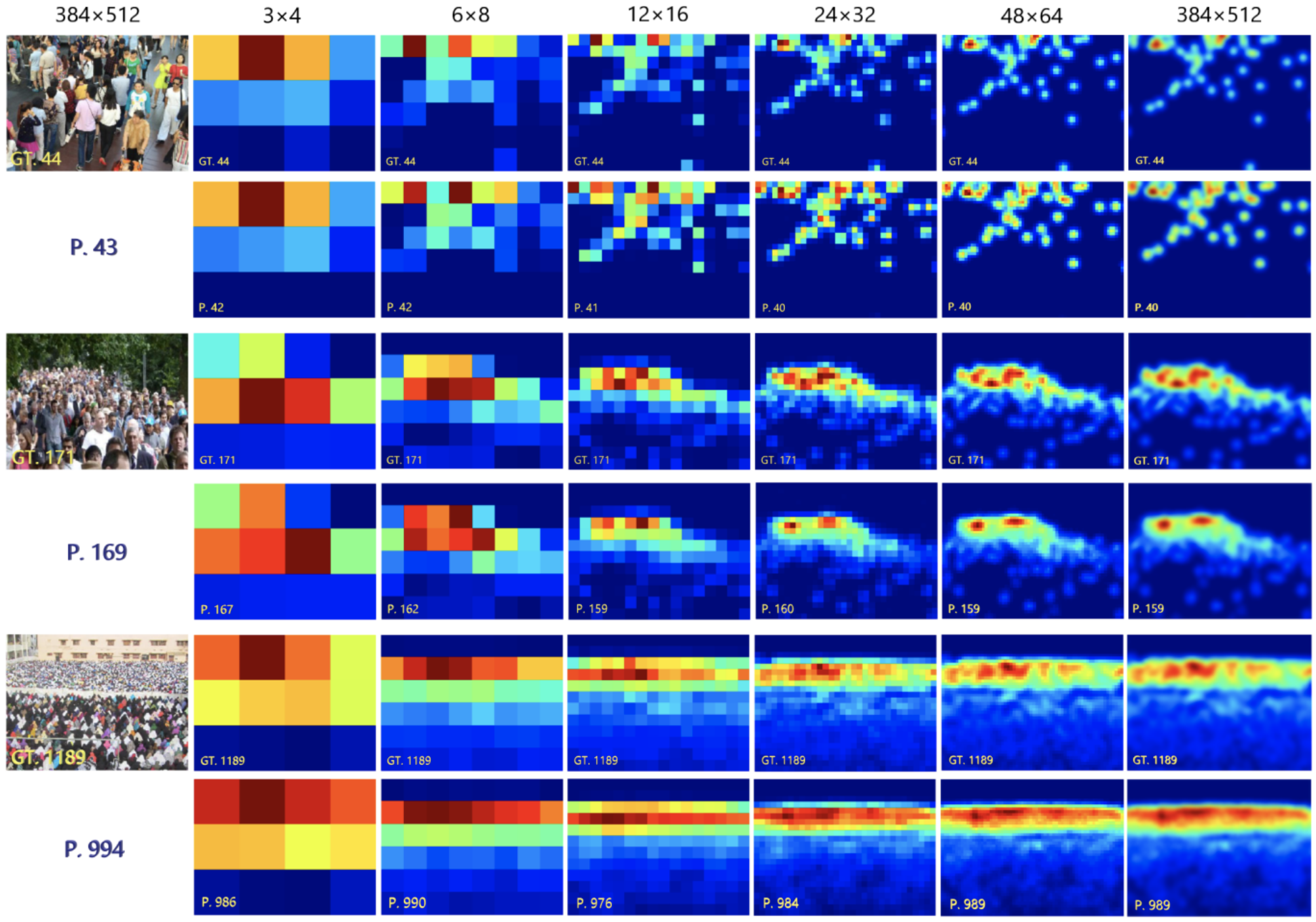
object detection, crowd counting aims at recognizing arbitrarily sized targets in various situations including sparse and cluttering scenes at the same time. Figure 1 illustrates
some of those challenging scenarios. In recent years, crowd counting has drawn more attention from computer vision researchers and has been in significant progress.
Early methods [7, 13, 33, 6, 17, 38] attempt to solve the problem by detecting every individual pedestrian in the crowd. These methods often perform poorly in the face of complex conditions such as those illustrated. The recent development of crowd counting comes from DNN-based methods which have achieved commendable performance. These
methods [37, 1, 32, 36, 2, 24, 20, 27, 29] concentrate on generating the demanding density maps before integrating them to the count. They are therefore categorised into density map-based methods. However, density maps have yet in effect to show too much importance in practice except for opportunely providing for demonstration, but are expensive
to compute, and their quality is difficult to guarantee. Meanwhile, methods that regress the global count directly have remained untouched for a while in research frontiers.
Raising state-of-the-art performances in many works, density maps have shown undeniable contribution to the improvement of prediction precision. One advantage of being
density map-based may be that information with respect to location, scale alike is fed to the network through density supervision. Consequently, multi-scale or multi-column
architectures [37, 1, 32, 2, 24] are usually adopted to fuse features from different scales to capture these kinds of information. Still, there exists two main drawbacks: first, computational cost drastically increases along with the growth of number of columns; second, useful information learned by low-level detectors might be lost through forward propagation. Likewise,
supervision information contained in gradients would be attenuated through backward propagation, making low-level detectors difficult to learn.
Figure 1: Representative images for challenges of non-uniform density, intra- and inter-scene variations in scale and perspective, and cluttering. In the figure, GT. means ground truth
and P. means prediction made by our model.
Besides, noise locally occurs due to uncertainty of annotation position on large-scale targets while Gaussian dispersion can only alleviate the issue to short extend. On the contrary,
a global count is immune to local noise, but does not carry location information which can be crucial for the network to develop attention on elusive targets.
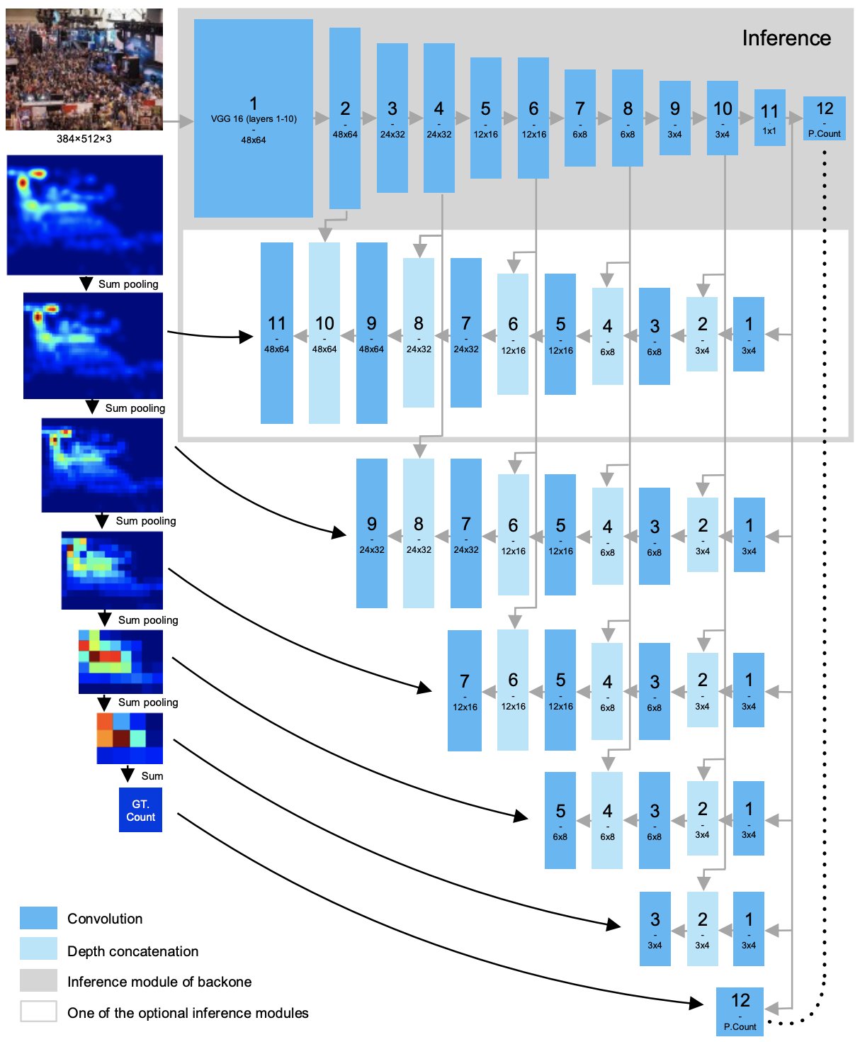
To address these problems, we propose a novel Gradient Fusion based model called DeepCount for crowd counting (network architecture shown in Figure 2), making efforts to both
avert expenditure of multi-column architecture and enhance resistance to local annotation noise. As in Figure 2, our proposed model contains a backbone network with convolution
layers deeply regressing a global count. Some auxiliary modules branch out to produce density maps with corresponding spatial dimensions and to feed gradients back to the backbone.
There are five branches having different depths and independent parameters so as to learn features in different aspects. Each branch will directly access different levels of the backbone to
inculcate knowledge to it deeply and make it more perceptive on the density distribution of the image, namely to be density-aware.
In inference phase, the backbone network can be used unaccompanied by any branches as a regressor to solely predict the global count at fastest speed, or, if needed, with
an auxiliary branch to also visualise a density map. Expensive computation is taken out, but with functionality promised.
Compared to other multi-column methods, our model fuses gradients other than features and avoids relying on the noisily supervised and computationally expensive density maps to
make prediction. By so doing, our model incorporates advantages of accuracy, flexibility, and efficiency.
Extensive experimental results on four benchmark datasets demonstrate significant improvements of our method against the state-of-the-art methods on Shanghai Tech Part A, Part B and
UCF-QNRF datasets and excellent performance on Mall dataset.
The rest of the paper is structured as follow: we review literatures for crowd counting in section 2; section 3 provides the detailed interpretation of our method; section 4 reports experiment results;
in section 5, we further discuss our findings and insights; the paper is to be concluded in section 6.
2 Related works
2.1 Detection-based methods
Early crowd counting methods tend to rely on detection approach. Low-level hand-crafted features such as Histograms of Oriented Gradients, silhouette-oriented features are exploited for traditional classifiers
such as Support Vector Machine and Random Forest [7, 33, 6, 17, 38]. Following are CNN-based methods (e.g. Faster R-CNN [25]) which have shown credible precision [19]. Nonetheless, in such times when the subject of crowd counting was more on the stage of pedestrian detection, performances of these methods on highly dense crowd scenes were similarly limited.
2.2 Count regression-based methods
Count regression-based methods are proposed to overcome limits encountered by detection-based methods. The idea of these methods is to regress a global count from the input image. There are methods using
ridge regression [4, 3], log-linear regression [22] or MLP [16] on low-level hand-crafted features to estimate the count. While they work satisfactorily on invariant scenes of sparse density, hand-crafted features can hardly represent enough variance and intricacy in complex counting scenarios. Alternatively, with the development of deep learning, features can be black-boxed and deeply learned to target the goal. Early success of
applying deep learning methods on crowd counting would be the end-to-end deep CNN regression model by Wang et al. [34]. Though, deep learning methods quickly narrowed onto density map-based methods which
have prevailed over the years since, and it was not until recently in [14] that Idrees et al. reported excellent experiment results on global count regression by advanced CNNs: Resnet101 [9] and Densenet201 [11], notwithstanding their focus on density map estimation.
2.3 Density map-based methods
Rodriguez et al. [26] first suggest the use of density map can improve crowd counting results significantly. It is supported by Zhang et al. [36] whose model produces small density map patches as well as the patch count
at its last layer. Following this density map approach, Zhang et al. [37] propose a multi-column architecture (MCNN) to also address scale variance of the targets. Inspired by such, Cao et al. [2] introduce Scale Aggregation
Network (SANet) which aggregates multi-scale features and fuses them in every layer. Likewise, Switching-CNN [1] has independent columns of CNN similar to multi-column network with different receptive fields, and ic-CNN [24] aims at predicting high-resolution density maps with two branches. Another set of methods devote themselves to trace context information as well as other abstractions all in a bit to improve the predicted density maps [32, 20, 27, 29]. On the other hand, CSRNet [18] builds dilated convolution layers upon a VGG-16 [30] backbone straightforward without too many manoeuvres, yet it reports excellent results and therefore becomes more practiced at present.
Differently, our method embodies heterogeneity of multi-column methods and straightforwardness of CSRNet whilst appearing as an existence that is both regression-based and density map-based.
Figure 2: The architecture of the proposed DeepCount Model. Module in the grey box is the backbone regressor, below which are 5 branches predicting density maps. Large-size numbers on the blocks are
referred to in detailed configuration in Table 1, while numbers in smaller font indicate the feature map dimensions.
Table 1: Configuration of DeepCount network. In the table, Conv and Conv-tr mean convolution and transposed convolution respectively. The pattern represents the dimension of convolution kernel. S denotes strides.
Module
Backbone
Branch 1
Branch 2
Branch 3
Branch 4
Branch 5
Input
Image
1
VGG 16
Layers 1-10
Conv-tr-S1
Conv-tr-S1
Conv-tr-S1
Conv-tr-S1
Conv-tr-S1
2
Conv-S1
Depth
Concatenation
Depth
Concatenation
Depth
Concatenation
Depth
Concatenation
Depth
Concatenation
3
Conv-S2
Conv-tr-S2
Conv-tr-S2
Conv-tr-S2
Conv-tr-S2
Conv-S1
4
Conv-S1
Depth
Concatenation
Depth
Concatenation
Depth
Concatenation
Depth
Concatenation
5
Conv-S2
Conv-tr-S2
Conv-tr-S2
Conv-tr-S2
Conv-S1
6
Conv-S1
Depth
Concatenation
Depth
Concatenation
Depth
Concatenation
7
Conv-S2
Conv-tr-S2
Conv-tr-S2
Conv-S1
8
Conv-S1
Depth
Concatenation
Depth
Concatenation
9
Conv-S2
Conv-tr-S2
Conv-S1
10
Conv-S1
Depth
Concatenation
11
Conv-S1
Conv-S1
12
Fc
Output
P. Count
P. Density Map
P. Density Map
P. Density Map
P. Density Map
P. Density Map
3 DeepCount
3.1 Gradient Fusion
We regard our methodology of designing the network as Gradient Fusion. Multi-column methods such as MCNN[37] and CP-CNN[32] are feature fusion methods assembling different columns features from which are fused and gradients to which are separated. Fusing feature maps of multiple columns entails lots of computation overhead since each column cannot be without in order to make prediction. In contrast, the method of gradient fusion fuses only gradient matrices
in backpropagation during training. We acknowledge that similar mechanisms are implemented in many works where they may be called otherwise. We use the name Gradient Fusion here to serve descriptive purpose to distinguish our methodology
from other multi-column methods on crowd counting.
In our network configuration (see section 3.3), the backbone module is mostly shared with branches which produce different density maps of different scales. Multi-source gradients are fused together to train this critical backbone. Complexities of solving
location estimation still exists for optimization of the parameters of the backbone. This restricts the backbone to learn location information to help branches predict density maps. This is a process which instils density-awareness to the backbone.
3.2 Density map pixelation and improved SNR
It takes great effort to label ground truth coordinates for heads in crowded images. Even with extra focus, getting wrong is inevitable. This brings error to the ground truth density maps. The correct density value of any data point in an
original MN density map (corresponding to an MN image) is the signal of the data. We assume signal () is normally distributed and has non-zero mean ().
We also assume the noise () a normally distributed random variable. It has zero mean, and standard deviation ().
Density maps of different scales are produced by pixelating the original MN density map. Each pixelation operation is a sum pooling layer with both stride and window size equal 2. After levels of pixelation, a data point in the density map has signal mean
(1)
, and noise variance
(2)
Therefore, signal-to-noise ratio (SNR) of the density map at the pixelation level is computed as
(3)
where is some constant. Thus, SNR of the training data in terms of every single data point grows exponentially for every pixelation operation, which means smaller density maps give more accurate information about the counting. But, on the other hand, some of the location information is lost after pixelation. Our network design is to maximum advantage of pixelated density map, and at the same time avoid any location information loss.
3.3 Network configuration
In order to signify our central point by comparing our model to others, we demonstrate a relatively simple network design in this paper. As shown in Figure 2, our proposed model consists of a straightforward down-sampling backbone and five branches interconnected to it. The backbone by itself has relatively low complexity. It functions as a deep CNN regressor which takes the crowd image as input and predicts the global count by regression. We design the network to have input size of to cater most aspect ratios in practical uses, whereas arbitrary larger input image sizes are tackled by division and combination. Correspondingly, there are density maps of sizes {} produced.
Specifically, the backbone has a frontend which extracts features from the input image. We transplant the first ten convolution layers from pretrained VGG-16 as our frontend model similar to CSRNet[18]. The frontend produces feature maps of 8 times smaller spatial width and height relative to the input. Following are some convolution layers to further dwindle the size of feature maps until when its spatial dimension matches the input dimension of a convolution layer entering to produce a vector. We use convolution with strides of 2 to halve the spatial dimension of the feature maps in the backend. In addition, a standard convolution layer is put between two down-sampling layers to further deepen the network and to smooth the reduction of features.
As for branches, they work in an up-sampling manner. Branches stemming from the last feature layer () of the backbone use transposed convolutions to up-sample the feature maps. To the output of each transposed convolution layer the deeper feature maps from backbone with the same dimension are channel-wise appended. Together, they form the input to the next transposed convolution layer. convolution is used to reconstruct channels to produce density map prediction. At the end of the backbone, a scalar value is produced as the global count prediction. We call our network DeepCount in short for deep CNN count regressor. Table 1 details the network configuration.
3.4 Generating ground truth density maps
To produce ground truth density maps for training, we first apply convolution by fixed Gaussian kernel with standard deviation = 5 (on the contrary of geometry-adaptive kernel adopted in most works) to generate density map of the same resolution as the original image, before sum pooling is employed to produce different levels of pixelated density maps. Five density maps are produced. Element sum of the density map is the ground truth count of the image.
3.5 Objective function
Labelling congested crowd data is indeed a painstaking task for human annotators. In some highly congested cases where the factual number of people is inevitably untraceable. This results in many annotations in congestions themselves being estimations and the ground truths becomes noisy. Also, for large scale heads, the annotation position is difficult to be exact. Hence, L1-norm loss is adopted to enhance robustness against noise as well as to convey steady updates to the network. We first define our objective function as:
(4)
where is the size of the training batch, enumerates outputs of all branches and the global count regressor, is the ground truth density map (or the global count when ), is the input image and denotes all parameters in model that contribute to making the corresponding prediction.
Given this objective function as basis, we add a multiplier to accentuate the importance of the global count prediction on backbone (where ). We notate it as a function of :
(5)
Moreover, we add another hyperparameter to approximately adjust the loss to a reasonably small value (10). An L2 regularisation term is also added to the function in an attempt to reduce overfitting. Hence, the objective function finally becomes:
(6)
3.6 Implementation
VGG-16 model pretrained on ImageNet is used to initialise the frontend of the backbone. Therefore, input images are normalised in the same manner as how the VGG-16 model is trained. As for initialising the remaining part of the model, we use Xavier [8] initialisation for weights and a constant value 0 for biases. With the exception of the VGG-16 frontend where ReLU is the activation function, we set parametric ReLUs (leaky ReLU):
(7)
following every convolution layer. We sweep hyperparameters and choose and
for the objective function in equation (6), and for the activation parameter [35] in equation (7). We use Gradient Descent optimisation with momentum 0.9 and initial learning rate to train our model, except for pretrained parameters in frontend where learning rate is divided by a factor of 2 to initially , Batch size is set to 32. On benchmark datasets, we train the network for around a hundred epochs.
As alluded to above, to cope with images of varied sizes, we divide the original image to crops to feed into our network. In inference, results from cropped images are to be merged to assemble the original ones again.
4 Evaluation
In this section, we report evaluation results yielded by our method introduced above. We evaluate our DeepCount network on four different public datasets: Shanghai Tech Part A and Part B [37], UCF-QNRF [14] and Mall [4]. Training details for all datasets are the same as mentioned in implementation section (section 3.6). In order to make fair comparison with benchmark results, we do no more data augmentation than random cropping and mirroring during training.
4.1 Evaluation metrics
For evaluation, we compute mean-absolute error (MAE) and root-mean-squared error (RMSE):
(8)
(9)
where is the number of testing images, and meaning predicted count and ground truth count respectively.
4.2 Shanghai Tech
Shanghai Tech[37] dataset includes Part A and Part B. Part A is the dataset for congested crowd counting. It has 241,677 annotations in 300 training images and 182 testing images with an average number 501. On the other hand, images in Part B are relatively sparse and all taken from streets in Shanghai. Our DeepCount model achieves state-of-the-art performance on both datasets. Test results are shown in Table 2.
Table 2: Test results on Shanghai Tech Part A and Part B.
The UCF-QNRF [14] dataset has a greater number of annotations (1,251,642) in higher quality images of a wider variety of scenes, including sparse and dense ones. There are extremely dense scenes in this dataset, so much so that a single image may have maximumly 12,865 of annotations in UCF-QNRF. It is considered a harder one. Our method outperforms current methods (see Table 4).
Table 3: Comparing between configurations and FLOPs of CSRNet and our DeepCount. Branch one (middle column) predicts the same- size density maps as does CSRNet, while backbone predicts a global count without producing any density maps.
Unlike the above datasets, images from Mall dataset[4] are surveillance video frames from a static viewpoint at a same venue. There are 800 frames for training and the other 1200 for testing. Since crowds in the dataset are sparse, Mall is not as challenging as others. Although previous methods have shown very promising results on this dataset, we still evaluate our model on it to demonstrate its excellent performance on invariant scene and as well to make comparison with some detection-based methods. (see Table 5).
Figure 3: Examples of ground truths and output density maps of test data from Shanghai Tech Part B (top), Part A (middle), UCF-QNRF (bottom). Density maps in the row starting with an image are the ground truths. The ones below are the predictions. The number in blue below the image is the predicted global count by backbone alone. The last column shows original size ground truth density maps and prediction density maps up-sampled from outputs of branch one, up-sampling being done by bilinear interpolation and separable Gaussian filter.
5 Discussion
5.1 Capacity and velocity
Arguably, the more parameters a neural network has, the greater its potential is to have high capacity to model the underlying relationship of the random variables. Although many cases suggest otherwise, we do often see positive correlation between extra parameters and increments of performance[18, 30, 9, 10]. Be that as it may, we still tend to avoid expensive computation a larger network would bear in practice. Trading off between capacity and velocity has been a dilemma for long. Hereby, we explicate how the idea of our DeepCount network is able to pursue both capacity and velocity at the same time by comparing it with CSRNet[18] in whose paper Li et al. argue cogently about the effect of number of parameters and design efficiency.
CSRNet and our backbone network use the same VGG-16 frontend. In the backend, CSRNet predicts the density map and our model predicts a global count. Assuming they receive the same input (backends thus receive input), we detail their layer configuration with corresponding output and computation cost of each layer in Table 3. In addition, we add branch one which predicts the same density map as CSRNet to the table. Computation cost is calculated in terms of number of floating-point operations (FLOPs) that happens throughout a forward pass in the backend. Number of FLOPs of one convolution layer is computed as:
(10)
where it depends multiplicatively upon output feature map size , convolution kernel size , number of output channels , and number of input channels .
Table 6: Comparing number of parameters and inference speed between CSRNet and the backbone of our DeepCount model.
Method
SHT Part B
MAE
Million
Parameters
FPS
Speedup
CSRNet
10.6
16.3
33
DeepCount(Ours)
7.2
21.4
(58.1 in total)
45
We also measure number of parameters as well as frame-per-second (FPS) for both networks (see Table 6). Run time evaluation is performed on one NVIDIA Tesla P40 GPU. As mentioned above, the backbone of our DeepCount model can be a standalone network detached from the rest in inference, and thereby becomes a count regressor without computing the computationally expensive density maps, and noticeably with better performance compared to other approaches.
As shown in Table 3 and Table 6, having a deeper architecture and greater preponderance of parameters (58.1 million for training and 21.4 million for inference) though, our DeepCount backbone does count inferences with much less FLOPs and therefore in higher velocity, and perhaps more importantly, with higher accuracy. These quantitative results suggest our proposed DeepCount model has the ability of accommodating more variations while making faster and better prediction. This implies its nature of outstanding capacity and efficiency.
5.2 Comparison on branches
Table 7: Comparing between outputs on different branches.
Branch 1
Branch 2
Branch 3
Branch 4
Branch 5
Backbone
Output Size
Million FLOPs
6034
2152
541
138
38
-
Shanghai Tech Part A
79.2
73.4
69.7
66.7
65.8
65.2
Shanghai Tech Part B
9.7
8.9
8.0
7.4
7.2
7.2
UCF-QNRF
193.3
185.0
155.3
112.3
96.9
95.7
Mall
4.74
2.89
2.46
1.77
1.56
1.55
As we have obtained the global count regressed by backbone, we can as well integrate the output density map to make count prediction like common density map-based methods. In the following, we compare predictions made between branches on MAE. Besides, we compute FLOPs for each branch to analyse their computational costs. Results are shown in Table 7.
As shown, the larger the density map, the harder it is to be precise. Immediate reasons for this may be that larger density maps are sparser and usually awash with noise caused mostly by annotations of large-scale heads. Our method avoids predicting the count relying merely on density maps but exploits useful information from them to rather train the global count regressor. This allows more accurate predictions to be achieved.
Despite extra computation, there are situations in which density map, which gives extra information about the distribution, becomes a requirement. Our model can make directly count inference with backbone at its full speed while optionally producing density maps of multiple resolutions. User can choose smaller density maps to reduce computational expensiveness or larger ones to get more illuminating impression about the crowd distribution. Using bilinear interpolation and separable Gaussian filter, the largest density map produced can be efficiently up-sampled to original resolution for high-definition display, thus we argue it is unworthy to train a network to produce a high-resolution density map. Figure 3 shows our predicted density maps compared to their ground truths.
5.3 Significance of gradients
Gradients are considered crucial to the achievement of our model. Hence, we detail more experiments to further cast light on the importance of them.
Since derivatives of ReLU are a staircase function suppressing the negative direction, gradients in half of its activation space are set to naught. The back-propagation gradient matrices are sparse and may hinder propagation of gradient flow and counterproductively cause a large part of the network underused. Instead, Parametric ReLU has non-zero gradients in all quadrants allowing the network to fully learn. Table 8 shows results of training a network with all ReLU activations in comparison with our baseline network. As shown in Table 8, when gradients are sparse, the capability of the network drops.
Table 8: Comparing results between using ReLU(sparse gradients) and PReLU(full gradients).
Activation
SHT Part B MAE
ReLU
8.3
PReLU
7.2
Also, the idea of being density-aware by gradient fusion is to leverage gradients sourced from supervision of multi-scale density maps. In ablation experiments (see Table 9), as we detach branches one by one from the largest to the smallest in training, the backbone receives less gradients in each case, and then the trend of performance degradation becomes more and more apparent. We also find that the model results satisfactorily when even trained with only global count on a dense dataset, while on a difficult one (sparse, non-uniform) it does not converge always, but we see it resolve if pretrained on dense dataset.
Table 9: Ablation on branches.
Ablation
SHT Part B MAE
No ablation
7.2
Branch 1 ablated
7.4
Branch 1-2 ablated
7.7
Branch 1-3 ablated
8.2
Branch 1-4 ablated
8.3
Branch 1-5 ablated
9.1
By means of this, we are now safer to conclude that the abundance of gradients has advantageous influence on our network and parameters in branches are indeed instrumental in the training of backbone. Giant as it may be, the network of branches is not a concern in an inference deployment. Unless training efficiency is also in a serious consideration, having a rationally greater number of parameters in this auxiliary module should be deemed innocuous as long as performance does not remain stagnant.
6 Conclusion
In this paper, we discuss advantages and limitations of current crowd counting methods, in light of which we propose a novel DeepCount network to be both fast and precise on count prediction and flexible on density map generation. State-of-the-art performance on public datasets evidences the effectiveness of our method. Our code is publicly available at:
https://github.com/GeorgeChenZJ/deepcount
We would like to thank the anonymous reviewers for their thoughtful
reading and comments.
References
[1]
Deepak Babu Sam, Shiv Surya, and R Venkatesh Babu, ‘Switching convolutional
neural network for crowd counting’, in Proceedings of the IEEE
Conference on Computer Vision and Pattern Recognition, pp. 5744–5752,
(2017).
[2]
Xinkun Cao, Zhipeng Wang, Yanyun Zhao, and Fei Su, ‘Scale aggregation network
for accurate and efficient crowd counting’, in Proceedings of the
European Conference on Computer Vision (ECCV), pp. 734–750, (2018).
[3]
Antoni B Chan, Zhang-Sheng John Liang, and Nuno Vasconcelos, ‘Privacy
preserving crowd monitoring: Counting people without people models or
tracking’, in 2008 IEEE Conference on Computer Vision and Pattern
Recognition, pp. 1–7. IEEE, (2008).
[4]
Ke Chen, Chen Change Loy, Shaogang Gong, and Tony Xiang, ‘Feature mining for
localised crowd counting.’, in BMVC, volume 1, p. 3, (2012).
[5]
Jifeng Dai, Yi Li, Kaiming He, and Jian Sun, ‘R-fcn: Object detection via
region-based fully convolutional networks’, in Advances in neural
information processing systems, pp. 379–387, (2016).
[6]
Juergen Gall, Angela Yao, Nima Razavi, Luc Van Gool, and Victor Lempitsky,
‘Hough forests for object detection, tracking, and action recognition’, IEEE transactions on pattern analysis and machine intelligence, 33(11), 2188–2202, (2011).
[7]
Weina Ge and Robert T Collins, ‘Marked point processes for crowd counting’, in
2009 IEEE Conference on Computer Vision and Pattern Recognition, pp.
2913–2920. IEEE, (2009).
[8]
Xavier Glorot and Yoshua Bengio, ‘Understanding the difficulty of training deep
feedforward neural networks’, in Proceedings of the thirteenth
international conference on artificial intelligence and statistics, pp.
249–256, (2010).
[9]
Kaiming He, Xiangyu Zhang, Shaoqing Ren, and Jian Sun, ‘Deep residual learning
for image recognition’, in Proceedings of the IEEE conference on
computer vision and pattern recognition, pp. 770–778, (2016).
[10]
Andrew G Howard, Menglong Zhu, Bo Chen, Dmitry Kalenichenko, Weijun Wang,
Tobias Weyand, Marco Andreetto, and Hartwig Adam, ‘Mobilenets: Efficient
convolutional neural networks for mobile vision applications’, arXiv
preprint arXiv:1704.04861, (2017).
[11]
Gao Huang, Zhuang Liu, Laurens Van Der Maaten, and Kilian Q Weinberger,
‘Densely connected convolutional networks’, in Proceedings of the IEEE
conference on computer vision and pattern recognition, pp. 4700–4708,
(2017).
[12]
Haroon Idrees, Imran Saleemi, Cody Seibert, and Mubarak Shah, ‘Multi-source
multi-scale counting in extremely dense crowd images’, in Proceedings of
the IEEE conference on computer vision and pattern recognition, pp.
2547–2554, (2013).
[13]
Haroon Idrees, Khurram Soomro, and Mubarak Shah, ‘Detecting humans in dense
crowds using locally-consistent scale prior and global occlusion reasoning’,
IEEE transactions on pattern analysis and machine intelligence, 37(10), 1986–1998, (2015).
[14]
Haroon Idrees, Muhmmad Tayyab, Kishan Athrey, Dong Zhang, Somaya Al-Maadeed,
Nasir Rajpoot, and Mubarak Shah, ‘Composition loss for counting, density map
estimation and localization in dense crowds’, in Proceedings of the
European Conference on Computer Vision (ECCV), pp. 532–546, (2018).
[15]
Xiaolong Jiang, Zehao Xiao, Baochang Zhang, Xiantong Zhen, Xianbin Cao, David
Doermann, and Ling Shao, ‘Crowd counting and density estimation by trellis
encoder-decoder networks’, in Proceedings of the IEEE Conference on
Computer Vision and Pattern Recognition, pp. 6133–6142, (2019).
[16]
Dan Kong, Douglas Gray, and Hai Tao, ‘A viewpoint invariant approach for crowd
counting’, in 18th International Conference on Pattern Recognition
(ICPR’06), volume 3, pp. 1187–1190. IEEE, (2006).
[17]
Min Li, Zhaoxiang Zhang, Kaiqi Huang, and Tieniu Tan, ‘Estimating the number of
people in crowded scenes by mid based foreground segmentation and
head-shoulder detection’, in 2008 19th International Conference on
Pattern Recognition, pp. 1–4. IEEE, (2008).
[18]
Yuhong Li, Xiaofan Zhang, and Deming Chen, ‘Csrnet: Dilated convolutional
neural networks for understanding the highly congested scenes’, in Proceedings of the IEEE conference on computer vision and pattern
recognition, pp. 1091–1100, (2018).
[19]
Jiang Liu, Chenqiang Gao, Deyu Meng, and Alexander G Hauptmann, ‘Decidenet:
Counting varying density crowds through attention guided detection and
density estimation’, in Proceedings of the IEEE Conference on Computer
Vision and Pattern Recognition, pp. 5197–5206, (2018).
[20]
Lingbo Liu, Hongjun Wang, Guanbin Li, Wanli Ouyang, and Liang Lin, ‘Crowd
counting using deep recurrent spatial-aware network’, arXiv preprint
arXiv:1807.00601, (2018).
[21]
Yuting Liu, Miaojing Shi, Qijun Zhao, and Xiaofang Wang, ‘Point in, box out:
Beyond counting persons in crowds’, in Proceedings of the IEEE
Conference on Computer Vision and Pattern Recognition, pp. 6469–6478,
(2019).
[22]
Zheng Ma and Antoni B Chan, ‘Crossing the line: Crowd counting by integer
programming with local features’, in Proceedings of the IEEE Conference
on Computer Vision and Pattern Recognition, pp. 2539–2546, (2013).
[23]
Viet-Quoc Pham, Tatsuo Kozakaya, Osamu Yamaguchi, and Ryuzo Okada, ‘Count
forest: Co-voting uncertain number of targets using random forest for crowd
density estimation’, in Proceedings of the IEEE International Conference
on Computer Vision, pp. 3253–3261, (2015).
[24]
Viresh Ranjan, Hieu Le, and Minh Hoai, ‘Iterative crowd counting’, in Proceedings of the European Conference on Computer Vision (ECCV), pp.
270–285, (2018).
[25]
Shaoqing Ren, Kaiming He, Ross Girshick, and Jian Sun, ‘Faster r-cnn: Towards
real-time object detection with region proposal networks’, in Advances
in neural information processing systems, pp. 91–99, (2015).
[26]
Mikel Rodriguez, Ivan Laptev, Josef Sivic, and Jean-Yves Audibert,
‘Density-aware person detection and tracking in crowds’, in 2011
International Conference on Computer Vision, pp. 2423–2430. IEEE, (2011).
[27]
Deepak Babu Sam and R Venkatesh Babu, ‘Top-down feedback for crowd counting
convolutional neural network’, in Thirty-Second AAAI Conference on
Artificial Intelligence, (2018).
[28]
Biyun Sheng, Chunhua Shen, Guosheng Lin, Jun Li, Wankou Yang, and Changyin Sun,
‘Crowd counting via weighted vlad on a dense attribute feature map’, IEEE Transactions on Circuits and Systems for Video Technology, 28(8),
1788–1797, (2016).
[29]
Zenglin Shi, Le Zhang, Yun Liu, Xiaofeng Cao, Yangdong Ye, Ming-Ming Cheng, and
Guoyan Zheng, ‘Crowd counting with deep negative correlation learning’, in
Proceedings of the IEEE conference on computer vision and pattern
recognition, pp. 5382–5390, (2018).
[30]
Karen Simonyan and Andrew Zisserman, ‘Very deep convolutional networks for
large-scale image recognition’, arXiv preprint arXiv:1409.1556, (2014).
[31]
Vishwanath A Sindagi and Vishal M Patel, ‘Cnn-based cascaded multi-task
learning of high-level prior and density estimation for crowd counting’, in
2017 14th IEEE International Conference on Advanced Video and Signal
Based Surveillance (AVSS), pp. 1–6. IEEE, (2017).
[32]
Vishwanath A Sindagi and Vishal M Patel, ‘Generating high-quality crowd density
maps using contextual pyramid cnns’, in Proceedings of the IEEE
International Conference on Computer Vision, pp. 1861–1870, (2017).
[33]
Paul Viola, Michael J Jones, and Daniel Snow, ‘Detecting pedestrians using
patterns of motion and appearance’, International Journal of Computer
Vision, 63(2), 153–161, (2005).
[34]
Chuan Wang, Hua Zhang, Liang Yang, Si Liu, and Xiaochun Cao, ‘Deep people
counting in extremely dense crowds’, in Proceedings of the 23rd ACM
international conference on Multimedia, pp. 1299–1302. ACM, (2015).
[35]
Bing Xu, Naiyan Wang, Tianqi Chen, and Mu Li, ‘Empirical evaluation of
rectified activations in convolutional network’, arXiv preprint
arXiv:1505.00853, (2015).
[36]
Cong Zhang, Hongsheng Li, Xiaogang Wang, and Xiaokang Yang, ‘Cross-scene crowd
counting via deep convolutional neural networks’, in Proceedings of the
IEEE conference on computer vision and pattern recognition, pp. 833–841,
(2015).
[37]
Yingying Zhang, Desen Zhou, Siqin Chen, Shenghua Gao, and Yi Ma, ‘Single-image
crowd counting via multi-column convolutional neural network’, in Proceedings of the IEEE conference on computer vision and pattern
recognition, pp. 589–597, (2016).
[38]
Tao Zhao, Ram Nevatia, and Bo Wu, ‘Segmentation and tracking of multiple humans
in crowded environments’, IEEE transactions on pattern analysis and
machine intelligence, 30(7), 1198–1211, (2008).