跳到论文正文
W Papers独立论文阅读器 arXiv:1908.03298 论文正文 计算阅读时间 · 0%
引用这篇论文根据当前论文元数据生成,正式投稿前建议核对。


License: arXiv.org perpetual non-exclusive license
arXiv:1908.03298v1 [cs.IT] 09 Aug 2019

On the Fundamental Limits of MIMO Massive Access CommunicationThanks: This paper was presented in part at IEEE ICC 2019. Y. Wu and W. Chen are the corresponding authors of this paper.Thanks: F. Wei and W. Chen are with Shanghai Institute of Advanced Communications and Data Sciences, the Department of Electronic Engineering, Shanghai Jiao Tong University, Minhang 200240, China (E-mail: weifan89@sjtu.edu.cn; wenchen@sjtu.edu.cn).Thanks: Y. Wu is with the Department of Electronic Engineering, Shanghai Jiao Tong University, Minhang 200240, China (e-mail: yongpeng.wu@sjtu.edu.cn)Thanks: Y. Geng is with State Key Lab of ISN, Xidian University, Xi’an, China (e-mail: ylgeng@xidian.edu.cn)Thanks: G. Caire is with Institute for Telecommunication Systems, Technical University Berlin, Einsteinufer 25, 10587 Berlin, Germany (Email: caire@tu-berlin.de).

Fan Wei    Yongpeng Wu    Affiliation: Wen Chen, , Yanlin Geng, , Affiliation: and Giuseppe Caire, 
Abstract

The multiple access channel (MAC) with many-user is a general model for massive machine type communications. In this paradigm, the number of users may be comparable or even larger than the coding blocklength nn. In contrast, classical MAC often assumes fixed and small number of the users. In this paper, we consider the massive access channel with multiple antennas system, where the base station (BS) with multiple receiving antennas serves the users in a single cell. The magnitude of users is assumed to grow unbounded with nn. We investigate the achievable region of MIMO massive access channel, where among the total users, an unknown subset referred to active users may transmit data periodically. The asymptotic active user identification cost is also quantified. With the theoretical analysis, it was shown that given finite number of the receiving antennas, the individual rate for each user can be formulated as the sum rate multiplied by some specific factors, which correspond to the allocation of sum capacity. The successive decoding does not apply due to the interferences from growing unbounded users. Theoretical analysis shows that successive decoding works only when the number of receiving antennas goes to infinity with the increasing codelength.

Index Terms: 
MIMO massive access channel, capacity region, user identification, sparse recovery, successive decoding.

I Introduction

Massive machine type communication (mMTC) has found its applications to various practical scenarios, such as wireless sensor networks, Device to Device (D2D) communication, and Internet of Things (IoT). A typical communication scenario would be a large pool of devices, with the magnitude of which may range from thousands to millions are simultaneously served by base station (BS) within single or multiple cells. Meanwhile, the users may send signals with a certain probability due to the sporadic traffic. When no data need to be delivered, the devices are kept in a sleep mode in order to save energy. Such communication scenarios have arisen two key differences from conventional multiple access (MAC) channels. In the first place, the conventional MAC assumes a fixed and small number of users such that the coding blocklength goes to infinity before the number of users operates in a same way. In contrast, in massive access communications, the number of active users may be comparable or even larger than the coding blocklength. In the second place, since the devices transmit data sporadically with certain probabilities, the decoder must be able to identify the set of active users before decoding, whereas in conventional MAC accurate user activity information is presumed.

To accommodate the such features, a many-access channel (MnAC) model was introduced in [1, 2, 3]. The key difference between MnAC and conventional MAC is that in MnAC, the number of active users may be comparable or even larger than the coding blocklength. The setup suggests a different approach to characterize the fundamental limits of MnAC. Mathematically, for a given number of users knk_{n}, which is a function of coding blocklength nn, limk→∞limn→∞f⁡(k,n)≠limn→∞f⁡(kn,n)\lim_{k\rightarrow\infty}\lim_{n\rightarrow\infty}f(k,n)\neq\lim_{n\rightarrow\infty}f(k_{n},n) for some functions f⁡(⋅)f(\cdot). The definition of MnAC model was introduced in [2]. There, it was shown random coding with Feinstein’s threshold decoding suffices to achieve the symmetric capacity of Gaussian MnAC, when knk_{n} grows sublinearly with nn. The linearly growing case was further investigated in [1], where the user identification cost for random access was also characterized. The technique for proof was based on Gallager’s error exponent analysis [4].

The models in MnAC [1, 2, 3] presume single antenna at both transceivers. On the other hand, wireless networks with multiple antennas [5, 6, 7, 8] simultaneously serving massive users is a promising 55G technology. In this paper, we investigate the achievable region of massive access channels with multiple antennas. The setup is akin to that in many-access channels. The difference is that multiple antenna arrays can be deployed at both transceivers. We characterize the asymmetric capacity of multiple-input multiple-output (MIMO) massive access channels, as well as the asymptotic user identification cost with random devices access. For the active devices identification, since active devices often constitute only a small subset of the potential ones, the sparse user recovery can be formulated as a compressed sensing problem [9, 10, 11, 12]. Thus, the user identification cost would be a by product of the asymptotic bound for sparse recovery in MIMO massive access channels. We derive the asymptotic user identification bound through concentration inequalities [13] which are related to the information density for signature symbols. From the viewpoint of communications, the derived compressed sensing bounds are further interpreted.

The asymmetric capacity for MIMO massive access channels when the set of active devices are known perfectly by the receiver is also investigated. We show that the rates can be formulated as the sum capacity of the system multiplied by some codebook size related factors that corresponds to the rate allocations. The asymptotic behavior of asymmetric capacity when the number of users goes to infinity is also characterized. Combining the results for user identification and data transmission, we finally obtain the finite dimension region of MIMO massive random access channels. In contrast to conventional MAC, where the achievable rates are determined by signal to interference plus noise (SINR), and are achieved by successive decoding at receiver [14], the successive interference cancellation may not be applicable in massive access channels given finite number of the receiving antennas. The underlying reason is by the growing unbounded user interferences in massive access channels [1]. As a last contribution of this paper, we further investigate the conditions for the number of receiving antennas required to be deployed when successive decoding works in MIMO massive access channels.

In addition to MnAC model, some recent works consider the user number KK may grow unbounded with the number of available resources NN, such that the overloading factor β=K/N\beta=K/N converges to some constant [15, 16, 17, 18]. The spectral efficiency for non-orthogonal multiple access (NOMA) with large system limit is investigated through the analysis of limiting spectral density of the spreading matrix [15]. Closed-form expression are further derived for optimal and linear minimum-mean-square error receivers, respectively [16]. The interesting results has suggested the superiority of regular sparse NOMA compared with the irregular one and also the dense randomly-spread code-division multiple-access, where the optimal decoding becomes prohibitive. Large system limit with fading scenario is further considered in [17].

It should be noted that the user random access is absent in the formulation of above models. For massive MIMO system, the achievable rates for massive connectivity with random user access are characterized in [19]. In contrast to this paper, the works in [19] assumes the number of receiving antennas may vary with user numbers such that the ratio between two quantities is kept fixed. Some practical schemes for user activity detection are further investigated in [20, 21]. In [22], random access code is defined such that the achievability bounds can be compared with existing schemes such as ALOHA, Code Division Multiple Access (CDMA), treating interference as noise (TIN), and etc. Some coding schemes [23, 24, 25] are considered later in order to achieve the above random code bound. A recent work [26] also considers the combining model of MnAC with the code definitions in [22], the bounds on the optimal required energy-per-bit is derived but with no considering on random access. For the MIMO system, a new scaling law has been investigated showing that given sufficient number of receiving antennas, the number of stably estimated active users may exceed the conventional one which is constrained by compressed sensing based user detection [27].

Unless otherwise noted, we use the following notational conventions: the lowercase letters xx, bold lowercase letters 𝐱\mathbf{x}, and bold uppercase letters 𝐗\mathbf{X} are used to denote scalars, column vectors, and matrices, respectively. We use (⋅)†(\cdot)^{\dagger} to denote complex conjugate and transpose for matrix and Tr​{⋅}\mbox{Tr}\{\cdot\} to denote the trace operator of matrix. The notion (nk)\binom{n}{k} denotes the binomial coefficient of nn choose kk. The binary entropy function is denoted by H2​(p)=−p​log⁡p−(1−p)​log⁡(1−p)H_{2}(p)=-p\log p-(1-p)\log(1-p). We use 𝒞​𝒩​(x,τ,υ)\mathcal{CN}(x;\tau,\upsilon) to denote xx follows complex Gaussian distribution with the mean τ\tau and variance υ\upsilon. The asymptotic notations O⁡(⋅)O(\cdot), o⁡(⋅)o(\cdot), Θ⁡(⋅)\Theta(\cdot), Ω⁡(⋅)\Omega(\cdot), and ω⁡(⋅)\omega(\cdot) follows a standard meaning [10]. The log⁡(⋅)\log(\cdot) functions are taken with natural base throughout this paper.

II System Model

II-A MIMO Massive Access Channels

We consider a MIMO massive access channels with ℓn\ell_{n} potential user equipments (UE) shown as in Fig. 1, where the receiver has NRN_{R} received antennas while the UEs are equipped with NTN_{T} transmit antennas. In the massive multiple access, the number of users is comparable or even larger than the coding blocklength nn. Therefore, unless dealing with the user identification problem, we denote ℓn\ell_{n} the number of potential users, and knk_{n} the number of active users on average, while the user transmission probability is given by αn=kn/ℓn\alpha_{n}=k_{n}/\ell_{n}. Since the UEs may be active or inactive depending on their data traffics, the uplink transmission can be divided into two phases. In the training phase, for the sake of user activity identification, the active UEs send signature signals to the base station (BS) with a signature length n0n_{0}. Thereafter, the active UEs send codewords with a coding blocklength n−n0n-n_{0} in the data transmission phase.

Let 𝒯={1,2,…,ℓn}\mathcal{T}=\{1,2,\ldots,\ell_{n}\} denote the total user set, and 𝒜⊆𝒯\mathcal{A}\subseteq\mathcal{T} denote the active UE set with the average size |𝒜||\mathcal{A}| equals kn=O⁡(n)k_{n}=O(n), the received signature signals at BS can be written as

𝐲⁡(i)\displaystyle\mathbf{y}(i) =∑k∈𝒜𝐇k​(i)​𝐬k​(i)+𝐳⁡(i)\displaystyle=\sum_{k\in\mathcal{A}}\mathbf{H}_{k}(i)\mathbf{s}_{k}(i)+\mathbf{z}(i) (1)
=∑k∈𝒯𝐇k​(i)​𝐬k​(i)​xk+𝐳⁡(i)\displaystyle=\sum_{k\in\mathcal{T}}\mathbf{H}_{k}(i)\mathbf{s}_{k}(i)x_{k}+\mathbf{z}(i) (2)
=𝐇(i)𝐒(i)𝐱+𝐳(i),i=1,2,…,n0\displaystyle=\mathbf{H}(i)\mathbf{S}(i)\mathbf{x}+\mathbf{z}(i),\,\,i=1,2,\ldots,n_{0} (3)

where 𝐇⁡(i)=[𝐇1​(i),𝐇2​(i),…,𝐇ℓn​(i)]\mathbf{H}(i)=\big[\mathbf{H}_{1}(i),\mathbf{H}_{2}(i),\ldots,\mathbf{H}_{\ell_{n}}(i)\big], and 𝐒⁡(i)=diag​{𝐬1​(i),𝐬2​(i),…,𝐬ℓn​(i)}\mathbf{S}(i)=\mbox{diag}\big\{\mathbf{s}_{1}(i),\mathbf{s}_{2}(i),\ldots,\mathbf{s}_{\ell_{n}}(i)\big\}. The matrix 𝐇k​(i)∈ℂNR×NT\mathbf{H}_{k}(i)\in\mathbb{C}^{N_{R}\times N_{T}} denotes the channel gain from UE kk, 𝐬k​(i)∈ℂNT\mathbf{s}_{k}(i)\in\mathbb{C}^{N_{T}} represents the signature symbols from UE kk, which is supposed to be independent and identically distributed (i.i.d.) according to complex Gaussian distribution, and 𝐳⁡(i)∈ℂNR\mathbf{z}(i)\in\mathbb{C}^{N_{R}} is the complex Gaussian noise with each entry from 𝒞​𝒩​(0,1)\mathcal{CN}(0,1). The Bernoulli vector 𝐱=[x1,x1,⋯,xℓn]T\mathbf{x}=[x_{1},x_{1},\cdots,x_{\ell_{n}}]^{T} follows since xkx_{k}s are the set of i.i.d. Bernoulli variables with probability αn=kn/ℓn\alpha_{n}=k_{n}/\ell_{n}. Given xk=1x_{k}=1, UE kk is active otherwise xk=0x_{k}=0.

Refer to caption
Fig. 1: MIMO massive random access network

For each channel use, the coefficient for each antenna within the channel matrix 𝐇k​(i)\mathbf{H}_{k}(i) can be formulated as

hl,m(k)​(i)=αl,m(k)​(i)​βk12,l∈[1,NR],m∈[1,NT],h_{l,m}^{(k)}(i)=\alpha_{l,m}^{(k)}(i)\beta_{k}^{\frac{1}{2}},\,\,l\in[1,N_{R}],\,m\in[1,N_{T}], (4)

where the small scale fading factor αl,m(k)​(i)\alpha_{l,m}^{(k)}(i) follows standard normal distribution 𝒞​𝒩​(0,1)\mathcal{CN}(0,1), and varies through different channel uses. On the other hand, the large scale fading βk\beta_{k} remains constant during the nn channel uses. For channel state information (CSI), we assume perfect knowledge of channel can be obtained at the receiver (CSIR) while only channel distribution information is available at the transmitter (CDIT).

Let 𝐗=𝐱⊗𝐈n0\mathbf{X}=\mathbf{x}\otimes\mathbf{I}_{n_{0}}, which denotes the Kronecker product of Bernoulli vector 𝐱={x1,x1,⋯xℓn}T\mathbf{x}=\{x_{1},x_{1},\cdots x_{\ell_{n}}\}^{T} and the identity matrix, the received signal in (3) can be rewritten as

𝐘n0=𝐇n0​𝐒n0​𝐗+𝐙n0=𝚽n0​𝐗+𝐙n0,\mathbf{Y}^{n_{0}}=\mathbf{H}^{n_{0}}\mathbf{S}^{n_{0}}\mathbf{X}+\mathbf{Z}^{n_{0}}=\mathbf{\Phi}^{n_{0}}\mathbf{X}+\mathbf{Z}^{n_{0}}, (5)

where 𝐘n0=[𝐲⁡(1),𝐲⁡(2),…,𝐲⁡(n0)]NR×n0\mathbf{Y}^{n_{0}}=\big[\mathbf{y}(1),\mathbf{y}(2),\ldots,\mathbf{y}(n_{0})\big]_{N_{R}\times n_{0}}, the channel and signature matrix are given by

𝐇n0=[𝐇⁡(1),𝐇⁡(2),⋯,𝐇⁡(n0)]NR×n0​NT​ℓn,\mathbf{H}^{n_{0}}=\begin{bmatrix}\mathbf{H}(1),&\mathbf{H}(2),&\cdots,&\mathbf{H}(n_{0})\\ \end{bmatrix}_{N_{R}\times n_{0}N_{T}\ell_{n}}, (6)

and

𝐒n0=[𝐒⁡(1)𝐒⁡(2)⋱𝐒⁡(n0)]n0​NT​ℓn×n0​ℓn,\mathbf{S}^{n_{0}}=\begin{bmatrix}\mathbf{S}(1)&&&\\ &\mathbf{S}(2)&&\\ &&\ddots&\\ &&&\mathbf{S}(n_{0})\\ \end{bmatrix}_{n_{0}N_{T}\ell_{n}\times n_{0}\ell_{n}}, (7)

respectively. Given ℓn≫kn\ell_{n}\gg k_{n}, the detection of sparse vector 𝐱\mathbf{x} can be formulated as a compressed sensing problem, where 𝚽n0=𝐇n0​𝐒n0\mathbf{\Phi}^{n_{0}}=\mathbf{H}^{n_{0}}\mathbf{S}^{n_{0}} is the sensing matrix.

The received data signals follows

𝐲ˇ(i)=∑k∈𝒯𝐇k(i)𝐬ˇk(i)+𝐳(i),i=n0+1,n0+2,…,n\check{\mathbf{y}}(i)=\sum_{k\in\mathcal{T}}\mathbf{H}_{k}(i)\check{\mathbf{s}}_{k}(i)+\mathbf{z}(i),\,\,i=n_{0}+1,n_{0}+2,\ldots,n (8)

where 𝐬ˇk​(i)∈ℂNT\check{\mathbf{s}}_{k}(i)\in\mathbb{C}^{N_{T}} denotes the transmitted codewords from user kk, and 𝐬ˇk​(i)=𝟎\check{\mathbf{s}}_{k}(i)=\mathbf{0} when user kk is inactive. The channel and Gaussian noise follow the analogous definitions as in Eq. (3).

II-B Codes Construction and Message-Length Capacity

In massive access channels, as the number of active users knk_{n} scales linearly with the codelength, the individual user rate would approach zero with fixed transmit powers and number of antennas due to the growing unbounded user interferences [14, Section 14.3]. As a consequence, the traditional notion of rate defined by R=log⁡M/n→0R=\log M/n\rightarrow 0 (where MM denotes the codebook size), i.e., bits per channel use becomes a less meaningful performance metric. To circumvent the above problem, we consider a codelength related notion for transmission rate, which is a referred to message-length capacity [1]. The following definitions introduce the asymmetric codes construction as well as the notion of message-length capacity for MIMO massive access channels.

Definition 1 (Codes Construction with Asymmetric Rate): Let 𝒮k\mathcal{S}_{k} and 𝒴\mathcal{Y} be the alphabet of input symbol for user kk and output symbol of the channel, respectively. An (M1,M2,…,Mℓn,n)(M_{1},M_{2},\ldots,M_{\ell_{n}},n) code for MIMO massive access channels (𝒮1×𝒮2×…×𝒮ℓn,PY|S1,…,Sℓn,𝒴)(\mathcal{S}_{1}\times\mathcal{S}_{2}\times...\times\mathcal{S}_{\ell_{n}},P_{Y|S_{1},...,S_{\ell_{n}}},\mathcal{Y}) consists of

  • •

    ℓn\ell_{n} sets of integers 𝒲k∈{0,1,2,…,Mk}\mathcal{W}_{k}\in\{0,1,2,...,M_{k}\} called message sets.

  • •

    The set of encoding functions ℰk:𝒲k→𝒮kNT×(n−n0)\mathcal{E}_{k}:\mathcal{W}_{k}\rightarrow\mathcal{S}^{N_{T}\times(n-n_{0})}_{k} for every user kk. For the set of active users, the transmitted codewords per channel use 𝐬k∈ℂNT×1\mathbf{s}_{k}\in\mathbb{C}^{N_{T}\times 1} should satisfy the following power constraint:

    pk−δ≤Tr⁡(𝐐k)≤pk,p_{k}-\delta\leq\mathrm{Tr}\big(\mathbf{Q}_{k}\big)\leq p_{k},

    where δ>0\delta>0 is an arbitrary small number and pk=Θ⁡(1)p_{k}=\Theta(1), i.e., a constant independent of the codelength nn, and 𝐐k=𝔼⁡{𝐬k​𝐬k†}\mathbf{Q}_{k}=\mathbb{E}\big\{\mathbf{s}_{k}\mathbf{s}_{k}^{{\dagger}}\big\} denotes the covariance matrix for codewords 𝐬k\mathbf{s}_{k}. For each user kk, the symbol 𝐬k\mathbf{s}_{k} are assumed to be generated i.i.d. according to the Gaussian distribution 𝒞​𝒩​(𝟎,𝐐k)\mathcal{CN}(\mathbf{0};\mathbf{Q}_{k}).

  • •

    A decoding function 𝒟:𝒴NR×(n−n0)→𝒲1×𝒲2×…×𝒲ℓn\mathcal{D}:\mathcal{Y}^{N_{R}\times(n-n_{0})}\rightarrow\mathcal{W}_{1}\times\mathcal{W}_{2}\times...\times\mathcal{W}_{\ell_{n}}, which is a deterministic mapping that assigns a sequence of estimated messages (𝒲1,𝒲2,…,𝒲ℓn)(\mathcal{W}_{1},\mathcal{W}_{2},...,\mathcal{W}_{\ell_{n}}) to each received vector 𝐘ˇ\check{\mathbf{Y}}.

The average error probability of the (M1,M2,…,Mℓn,n)(M_{1},M_{2},\ldots,M_{\ell_{n}},n) code is given by

Pe(n)=Pr{𝒟(𝐘ˇ(n−n0))≠(𝒲1,𝒲2,…,𝒲ℓn)},P_{e}^{(n)}=\mathrm{Pr}\big\{\mathcal{D}(\check{\mathbf{Y}}^{(n-n_{0})})\neq(\mathcal{W}_{1},\mathcal{W}_{2},\ldots,\mathcal{W}_{\ell_{n}})\big\}, (9)

where the messages (𝒲1,𝒲2,…,𝒲ℓn)(\mathcal{W}_{1},\mathcal{W}_{2},\ldots,\mathcal{W}_{\ell_{n}}) are generated independently over the message set, i.e.,

Pr{𝒲k=w}={1−αn,w=0;αn/Mk,w∈𝒲k\{0}.\mathrm{Pr}\{\mathcal{W}_{k}=w\}=\left\{\begin{array}[]{ll}1-\alpha_{n},&\hbox{$w=0$;}\\ \alpha_{n}/M_{k},&\hbox{$w\in\mathcal{W}_{k}\backslash\{0\}$.}\end{array}\right. (10)

Definition 2 (Asymptotically Achievable Message-Length): Given the set of functions Rk​(⋅)R_{k}(\cdot) that map natural numbers to some positive value, we say the message-length Rk​(n)R_{k}(n) are asymptotically achievable if there exists a sequence of (⌈exp⁡(R1​(n))⌉,⌈exp⁡(R2​(n))⌉,…,⌈exp⁡(Rℓn​(n))⌉,n)(\lceil\exp(R_{1}(n))\rceil,\lceil\exp(R_{2}(n))\rceil,\ldots,\lceil\exp(R_{\ell_{n}}(n))\rceil,n) codes in the sense of Definition 11 such that the average error probability Pe(n)P_{e}^{(n)} vanishes as n→∞n\rightarrow\infty.

The capacity region for MIMO massive access channels can be the closure sets of all achievable rate tuples (R1​(n),R2​(n),…,Rkn​(n))\big(R_{1}(n),R_{2}(n),\ldots,R_{k_{n}}(n)\big) for the knk_{n} active users. However, as nn becomes larger, the dimension of this rate tuple also increases since the number of users now grows unbounded with nn. Thus, to avoid an increasing dimension of capacity region, we define the finite dimension region of MIMO massive access channel by noting that the message set size MkM_{k} may not necessarily different from each other.

Definition 3 (Finite Dimension Message-Length Region): Let KjK_{j} denote the number of users with message set size exp⁡{Vj​(n)}\exp\{V_{j}(n)\}, i.e., with message-length rate Rk​(n)=Vj​(n)R_{k}(n)=V_{j}(n) for k∈𝒜k\in\mathcal{A}, where Vj​(n)V_{j}(n) are the set of “distinct” message-length rates in the system. Then by grouping together the rates Rk​(n)R_{k}(n) that are equal to each other, the JJ-dimensional region of MIMO massive access channel is defined as the closure of the convex hull of all (V1​(n),V2​(n),…,VJ​(n))\big(V_{1}(n),V_{2}(n),\ldots,V_{J}(n)\big), such that if ∑j=1JKj​Vj​(n)\sum_{j=1}^{J}K_{j}V_{j}(n) is upper bounded by the sum rate of the system, the error probability goes to zero asymptotically.

For the finite and denumerable message set size, the dimension JJ was expected to be independent of codelength nn. Thus, in Definition 3, a finite dimension region is formulated through the achievable rates for the given number of sustainable users.

III Main Results

In this subsection, the main results of this paper are stated by the following theorems. For the UE identification in the training phase, the BS outputs a set 𝒜^\hat{\mathcal{A}} with size |𝒜^|=kn|\hat{\mathcal{A}}|=k_{n}, which corresponds to the estimation of true set 𝒜\mathcal{A}. Due to the random access nature, the size of active user set 𝒜\mathcal{A} may vary randomly in every transmission. Let k𝒜=|𝒜|k_{\mathcal{A}}=|\mathcal{A}| be the random variable and δ>0\delta>0, by Chebyshev’s inequality,

Pr{|k𝒜−kn|≥δn}≤Vk𝒜δ2​n2,\mathrm{Pr}\big\{|k_{\mathcal{A}}-k_{n}|\geq\delta n\big\}\leq\frac{V_{k_{\mathcal{A}}}}{\delta^{2}n^{2}}, (11)

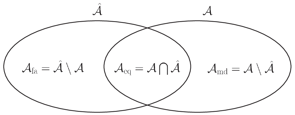
where Vk𝒜V_{k_{\mathcal{A}}} denotes the variance of random variable k𝒜k_{\mathcal{A}}. Eq. (11) indicates that for finite Vk𝒜V_{k_{\mathcal{A}}}, the probability that k𝒜k_{\mathcal{A}} deviates from the average number knk_{n} vanishes asymptotically as the codelength increases. Therefore in this paper, we assume that the decoded set 𝒜^\hat{\mathcal{A}} has almost the same cardinality with 𝒜\mathcal{A} on average. Fig. 2 illustrates the set relationship between 𝒜\mathcal{A} and 𝒜^\hat{\mathcal{A}}, where 𝒜eq\mathcal{A}_{\mathrm{eq}} denotes the correct decoded set, 𝒜fa\mathcal{A}_{\mathrm{fa}} denotes the false alarm set, and 𝒜md\mathcal{A}_{\mathrm{md}} corresponds to the misdetection set. Define the error decode probability as

Pe(ℓ)=Pr{𝒜^≠𝒜}.P^{(\ell)}_{e}=\mathrm{Pr}\{\hat{\mathcal{A}}\neq\mathcal{A}\}. (12)

To find the limits for UE identification, we assume ℓ→∞\ell\rightarrow\infty and let the other parameters change with ℓ\ell. Theorem 1 provides the asymptotic UE identification cost for the centralized detection schemes.
Refer to caption
Fig. 2: The relationship between sets 𝒜\mathcal{A} and 𝒜^\hat{\mathcal{A}}, where |𝒜|=|𝒜^|=kn|\mathcal{A}|=|\hat{\mathcal{A}}|=k_{n}, |𝒜md|=|𝒜fa|=i|\mathcal{A}_{\mathrm{md}}|=|\mathcal{A}_{\mathrm{fa}}|=i.

Theorem 1 (UE Identification Cost for Massive Random Access Channels): Denote the total number of users as ℓ\ell and the number of active users as kℓk_{\ell}. Suppose ℓ\ell and kℓk_{\ell} satisfy the following condition

limℓ→∞ℓ​e−ϱ​kℓ=0\lim_{\ell\rightarrow\infty}\ell e^{-\varrho k_{\ell}}=0 (13)

for all ϱ>0\varrho>0, which indicates that kℓ→∞k_{\ell}\rightarrow\infty as ℓ→∞\ell\rightarrow\infty. Let i=|𝒜md|i=|\mathcal{A}_{\mathrm{md}}|, if the asymptotic number of UE identification cost for centralized detection is given by

n0≥(1+ϵ)⋅maxi=1,…,kℓ⁡log⁡(ℓ−kℓi)𝔼𝐇{logdet(𝐈NR+∑k∈𝒜md𝐇k𝐐k𝐇†k)}n_{0}\geq(1+\epsilon)\cdot\max_{i=1,\ldots,k_{\ell}}\frac{\log\binom{\ell-k_{\ell}}{i}}{\mathbb{E}_{\mathbf{H}}\Big\{\log\det\big(\mathbf{I}_{N_{R}}+\sum\limits_{k\in\mathcal{A}_{\mathrm{md}}}\mathbf{H}_{k}\mathbf{Q}_{k}\mathbf{H}^{\dagger}_{k}\big)\Big\}} (14)

for some ϵ>0\epsilon>0, the error probability can be made Pe(ℓ)→0P^{(\ell)}_{e}\rightarrow 0 as ℓ\ell goes to infinity.

Conversely, when the asymptotic number of UE identification cost

n0≤(1−ϵ)⋅maxi=1,…,kℓ⁡log⁡(ℓ−kℓ+ii)𝔼𝐇{logdet(𝐈NR+∑k∈𝒜md𝐇k𝐐k𝐇†k)},n_{0}\leq(1-\epsilon)\cdot\max_{i=1,\ldots,k_{\ell}}\frac{\log\binom{\ell-k_{\ell}+i}{i}}{\mathbb{E}_{\mathbf{H}}\Big\{\log\det\big(\mathbf{I}_{N_{R}}+\sum\limits_{k\in\mathcal{A}_{\mathrm{md}}}\mathbf{H}_{k}\mathbf{Q}_{k}\mathbf{H}^{\dagger}_{k}\big)\Big\}}, (15)

for some ϵ>0\epsilon>0, we have Pe(ℓ)→1P^{(\ell)}_{e}\rightarrow 1 as ℓ\ell goes to infinity. □\square

After training phase, the receiver has a perfect knowledge of user activity within the network. The next phase is to decode the data from active UEs. Theorem 2 states the asymmetric rate for MIMO massive multiple access channels when the receiver knowing perfectly the true active UE set 𝒜\mathcal{A}.

Theorem 2 (Asymmetric Message-Length Rate for Massive Access Channels): For MIMO massive access channel described in (8), let 𝒜={1,2,…,kn}\mathcal{A}=\{1,2,\ldots,k_{n}\} denote the active user set in the network, where the total number of users scales as kn=O⁡(n)k_{n}=O(n). Assume the codebook size MkM_{k} for each user is on the same order, the message-length vector with components (R1​(n),R2​(n),…,Rkn​(n))\big(R_{1}(n),R_{2}(n),\ldots,R_{k_{n}}(n)\big) is asymptotically achievable if

Rk(n)≤ck𝔼𝐇{logdet(𝐈NR+∑t∈𝒜𝐇t𝐐t𝐇t†)},R_{k}(n)\leq c_{k}\mathbb{E}_{\mathbf{H}}\Big\{\log\det\big(\mathbf{I}_{N_{R}}+\sum_{t\in\mathcal{A}}\mathbf{H}_{t}\mathbf{Q}_{t}\mathbf{H}^{\dagger}_{t}\big)\Big\}, (16)

where ck=limn→∞n​μk(n)>0c_{k}=\lim\limits_{n\rightarrow\infty}n\mu_{k}^{(n)}>0, μk(n)=log⁡Mk∑t∈𝒜log⁡Mt∈(0,1)\mu_{k}^{(n)}=\frac{\log M_{k}}{\sum_{t\in\mathcal{A}}\log M_{t}}\in(0,1). □\square

Note that Theorem 2 has assumed that the codebook sizes MkM_{k} are on the same order for the users within the network, it then follows that 1/μkn=O⁡(n)1/\mu_{k}^{n}=O(n) and ∑k=1knck=n\sum_{k=1}^{k_{n}}c_{k}=n. Those two conditions may be useful in proving the theorems in later sections.

Corollary 1: In the massive access channels, given kn=O⁡(n)k_{n}=O(n), the asymptotically individual message-length rate behaves as

Rk​(n)→|𝒜|→∞\displaystyle R_{k}(n)\xrightarrow{|\mathcal{A}|\rightarrow\infty} ck​NR​log⁡(1+∑t∈𝒜βt​pt)\displaystyle\,c_{k}N_{R}\log\Big(1+\sum_{t\in\mathcal{A}}\beta_{t}p_{t}\Big) (17)
=\displaystyle= ck​NR​O​(log⁡n)+O⁡(1),\displaystyle\,c_{k}N_{R}O(\log n)+O(1), (18)

where pk=Tr⁡(𝐐k)p_{k}=\mathrm{Tr}(\mathbf{Q}_{k}). The term O⁡(log⁡n)O(\log n) is independent of any other constants but relates only to nn, and the O⁡(1)O(1) constant depends on the pathlosses and transmit powers. □\square

The result in (17) indicates that due to the effect of channel hardening, the asymptotic rate is close to that when the transmitter has only the statistic knowledge of effective channel gain.

Combining the results in Theorem 1 and Theorem 2, we have the following Theorem for the capacity with massive random access.

Theorem 3 (Asymmetric Message-Length Capacity for Massive Random Access Channels): Let the total number of user be ℓn\ell_{n}, and assume each user is active with a probability αn\alpha_{n} such that the average number of active users is kn=αn​ℓnk_{n}=\alpha_{n}\ell_{n}. Define

θn=ℓn​H2​(αn)n𝔼𝐇{logdet(𝐈NR+∑k∈𝒜md𝐇k𝐐k𝐇†k)}.\theta_{n}=\frac{\ell_{n}H_{2}(\alpha_{n})}{n\mathbb{E}_{\mathbf{H}}\Big\{\log\det\big(\mathbf{I}_{N_{R}}+\sum\limits_{k\in\mathcal{A}_{\mathrm{md}}}\mathbf{H}_{k}\mathbf{Q}_{k}\mathbf{H}^{\dagger}_{k}\big)\Big\}}. (19)

When 0<θn<10<\theta_{n}<1, kn=O⁡(n)k_{n}=O(n) and the scaling of ℓn\ell_{n} and knk_{n} follows (13), the asymmetric message-length capacity for user kk is given by

Bk(n)=ck𝔼𝐇{logdet(𝐈NR+∑t∈𝒜𝐇t𝐐t𝐇t†)}−μk(n)ℓnH2(αn),\displaystyle B_{k}(n)=c_{k}\mathbb{E}_{\mathbf{H}}\Big\{\log\det\big(\mathbf{I}_{N_{R}}+\sum_{t\in\mathcal{A}}\mathbf{H}_{t}\mathbf{Q}_{t}\mathbf{H}^{\dagger}_{t}\big)\Big\}-\mu_{k}^{(n)}\ell_{n}H_{2}(\alpha_{n}), (20)

where ckc_{k} and μk(n)\mu_{k}^{(n)} are defined in Theorem 2. □\square

Notice that for each user kk, rate (20) is determined by ckc_{k} (or MkM_{k}). Since the message set size MkM_{k} may not necessarily different from each other, given the Definition 3, the finite dimension region of MIMO massive access channel is formulated as

𝒞ℳ​𝒜​𝒞(n)≜{(V1(n),…,VJ(n)):K1V1(n)+⋯+KJVJ(n)\displaystyle\mathcal{C}_{\mathcal{MAC}}(n)\triangleq\Bigg\{\big(V_{1}(n),...,V_{J}(n)\big):K_{1}V_{1}(n)+\cdots+K_{J}V_{J}(n)
≤n𝔼𝐇{logdet(𝐈NR+∑k∈𝒜𝐇k𝐐k𝐇k†)}−ℓnH2(αn)},\displaystyle\leq n\mathbb{E}_{\mathbf{H}}\Big\{\log\det\big(\mathbf{I}_{N_{R}}+\sum_{k\in\mathcal{A}}\mathbf{H}_{k}\mathbf{Q}_{k}\mathbf{H}^{\dagger}_{k}\big)\Big\}-\ell_{n}H_{2}(\alpha_{n})\Bigg\}, (21)

where JJ denotes dimension of the region, which is independent of codelength nn.

IV Proof of Theorem 1 (UE Identification Cost)

IV-A Information Density and the Concentration Inequality

We begin this section by reviewing the concept of information density [28] and the related concentration inequalities [13]. For the received signal (5), let 𝐒𝒜n0={𝐒𝒜eqn0,𝐒𝒜mdn0}\mathbf{S}^{n_{0}}_{\mathcal{A}}=\{\mathbf{S}^{n_{0}}_{\mathcal{A}_{\mathrm{eq}}},\mathbf{S}^{n_{0}}_{\mathcal{A}_{\mathrm{md}}}\}, where we use 𝐒𝒜n0\mathbf{S}^{n_{0}}_{\mathcal{A}} to denote the submatrix containing the signals from user set 𝒜\mathcal{A} only. Given the joint probability P⁡(𝐘n0,𝐒𝒜n0,𝐇n0)P(\mathbf{Y}^{n_{0}},\mathbf{S}^{n_{0}}_{\mathcal{A}},\mathbf{H}^{n_{0}}), the conditional information density is defined as

ı(𝐘n0;𝐒𝒜mdn0|𝐒𝒜eqn0,𝐇n0)=logP⁡(𝐘n0|𝐒𝒜mdn0,𝐒𝒜eqn0,𝐇n0)P⁡(𝐘n0|𝐒𝒜eqn0,𝐇n0).\imath(\mathbf{Y}^{n_{0}};\mathbf{S}^{n_{0}}_{\mathcal{A}_{\mathrm{md}}}|\mathbf{S}^{n_{0}}_{\mathcal{A}_{\mathrm{eq}}},\mathbf{H}^{n_{0}})=\log\frac{P(\mathbf{Y}^{n_{0}}|\mathbf{S}^{n_{0}}_{\mathcal{A}_{\mathrm{md}}},\mathbf{S}^{n_{0}}_{\mathcal{A}_{\mathrm{eq}}},\mathbf{H}^{n_{0}})}{P(\mathbf{Y}^{n_{0}}|\mathbf{S}^{n_{0}}_{\mathcal{A}_{\mathrm{eq}}},\mathbf{H}^{n_{0}})}. (22)

Eq. (22) is referred to as (conditional) information density because when averaging with the joint probability P⁡(𝐘n0,𝐒𝒜n0,𝐇n0)P(\mathbf{Y}^{n_{0}},\mathbf{S}^{n_{0}}_{\mathcal{A}},\mathbf{H}^{n_{0}}), we obtain the conditional mutual information, i.e.,

𝔼P⁡(𝐘n0,𝐒𝒜n0,𝐇n0){ı(𝐘n0;𝐒𝒜mdn0|𝐒𝒜eqn0,𝐇n0)}=I(𝐘n0;𝐒𝒜mdn0|𝐒𝒜eqn0,𝐇n0).\mathbb{E}_{P(\mathbf{Y}^{n_{0}},\mathbf{S}^{n_{0}}_{\mathcal{A}},\mathbf{H}^{n_{0}})}\big\{\imath(\mathbf{Y}^{n_{0}};\mathbf{S}^{n_{0}}_{\mathcal{A}_{\mathrm{md}}}|\mathbf{S}^{n_{0}}_{\mathcal{A}_{\mathrm{eq}}},\mathbf{H}^{n_{0}})\big\}=\,I(\mathbf{Y}^{n_{0}};\mathbf{S}^{n_{0}}_{\mathcal{A}_{\mathrm{md}}}|\mathbf{S}^{n_{0}}_{\mathcal{A}_{\mathrm{eq}}},\mathbf{H}^{n_{0}}). (23)

Given the above definition, the following concentration inequality relates to the information density in (22) may be useful to prove of the theorems in Section II.

Lemma 1: For the arbitrary set partition 𝒜={𝒜eq,𝒜md}\mathcal{A}=\{\mathcal{A}_{\mathrm{eq}},\mathcal{A}_{\mathrm{md}}\}, let 𝐲,𝐬𝒜\mathbf{y},\mathbf{s}_{\mathcal{A}} denote the received and the transmit signals per channel use, respectively. Define 𝐆𝒜md=∑k∈𝒜md𝐇k​𝐐k​𝐇k†\mathbf{G}_{\mathcal{A}_{\mathrm{md}}}=\sum_{k\in\mathcal{A}_{\mathrm{md}}}\mathbf{H}_{k}\mathbf{Q}_{k}\mathbf{H}^{\dagger}_{k}, where 𝐇k\mathbf{H}_{k} denotes the random channel matrix for user kk in an arbitrary channel use. We then have the following concentration inequality for the signals in (5)

Pr{|ı(𝐘n0;𝐒𝒜mdn0|𝐒𝒜eqn0,𝐇n0)−n0I(𝐲;𝐬𝒜md|𝐬𝒜eq,𝐇)|≥n0δ}≤2exp{−n0​δ24​c2+2​c​δ},\displaystyle\mathrm{Pr}\Big\{\big|\imath(\mathbf{Y}^{n_{0}};\mathbf{S}^{n_{0}}_{\mathcal{A}_{\mathrm{md}}}|\mathbf{S}^{n_{0}}_{\mathcal{A}_{\mathrm{eq}}},\mathbf{H}^{n_{0}})-n_{0}I(\mathbf{y};\mathbf{s}_{\mathcal{A}_{\mathrm{md}}}|\mathbf{s}_{\mathcal{A}_{\mathrm{eq}}},\mathbf{H})\big|\geq n_{0}\delta\Big\}\leq 2\exp\Big\{-\frac{n_{0}\delta^{2}}{4c^{2}+2c\delta}\Big\}, (24)

where δ>0\delta>0, c=32NR+𝔼𝐇[det(𝐈NR+𝐆𝒜md)]e−I(𝐲;𝐬𝒜md|𝐬𝒜eq,𝐇)c=32N_{R}+\mathbb{E}_{\mathbf{H}}\Big[\det\big(\mathbf{I}_{N_{R}}+\mathbf{G}_{\mathcal{A}_{\mathrm{md}}}\big)\Big]e^{-I(\mathbf{y};\mathbf{s}_{\mathcal{A}_{\mathrm{md}}}|\mathbf{s}_{\mathcal{A}_{\mathrm{eq}}},\mathbf{H})} is some constant, and the mutual information is given by

I(𝐲;𝐬𝒜md|𝐬𝒜eq,𝐇)=𝔼𝐇{logdet(𝐈NR+∑k∈𝒜md𝐇k𝐐k𝐇k†)}.I(\mathbf{y};\mathbf{s}_{\mathcal{A}_{\mathrm{md}}}|\mathbf{s}_{\mathcal{A}_{\mathrm{eq}}},\mathbf{H})=\mathbb{E}_{\mathbf{H}}\Big\{\log\det\Big(\mathbf{I}_{N_{R}}+\sum_{k\in\mathcal{A}_{\mathrm{md}}}\mathbf{H}_{k}\mathbf{Q}_{k}\mathbf{H}^{\dagger}_{k}\Big)\Big\}. (25)

□\square

Proof: See Appendix A.

IV-B Proof of Achievability

Consider a maximum likelihood (ML) decoder for the active UE detection. Mathematically, the ML decoder is assumed to search an arbitrary subset 𝒜~⊆𝒯\tilde{\mathcal{A}}\subseteq\mathcal{T} with such that

𝒜≡𝒜^=arg⁡max𝒜~⊆𝒯⁡P⁡(𝐘n0|𝐒𝒜~n0,𝐇n0).\mathcal{A}\equiv\hat{\mathcal{A}}=\arg\max_{\tilde{\mathcal{A}}\subseteq\mathcal{T}}P(\mathbf{Y}^{n_{0}}|\mathbf{S}^{n_{0}}_{\tilde{\mathcal{A}}},\mathbf{H}^{n_{0}}). (26)

We define the error event

Ξi={∃𝒜^≠𝒜:P(𝐘n0|𝐒𝒜^n0,\displaystyle\Xi_{i}=\big\{\exists\,\hat{\mathcal{A}}\neq\mathcal{A}:P(\mathbf{Y}^{n_{0}}|\mathbf{S}^{n_{0}}_{\hat{\mathcal{A}}}, OPEN𝐇n0)>P⁡(𝐘n0|𝐒𝒜n0,𝐇n0),\displaystyle\,\mathbf{H}^{n_{0}})>P(\mathbf{Y}^{n_{0}}|\mathbf{S}^{n_{0}}_{\mathcal{A}},\mathbf{H}^{n_{0}}),
|𝒜fa|=|𝒜md|=i,|𝒜^|=|𝒜|=kℓ},\displaystyle|\mathcal{A}_{\mathrm{fa}}|=|\mathcal{A}_{\mathrm{md}}|=i,|\hat{\mathcal{A}}|=|\mathcal{A}|=k_{\ell}\big\}, (27)

for all i∈{1,…,kℓ}i\in\{1,\ldots,k_{\ell}\}, as there exists a kℓk_{\ell}-size set 𝒜^\hat{\mathcal{A}} that has resulted in ii false alarm users and ii misdetection users, and is deemed to be more likely by the decoder. The relationship between sets 𝒜^\hat{\mathcal{A}} and 𝒜\mathcal{A} is illustrated in Fig. 2.

Define the set Ψi\Psi_{i} as

Ψi={𝒜^⊆𝒯:|𝒜fa|=i,|𝒜eq|=kℓ−i},\Psi_{i}=\big\{\hat{\mathcal{A}}\subseteq\mathcal{T}:|\mathcal{A}_{\mathrm{fa}}|=i,|\mathcal{A}_{\mathrm{eq}}|=k_{\ell}-i\big\}, (28)

i.e., the collection of decoded sets 𝒜^\hat{\mathcal{A}} that result in ii false alarm users and ii misdetection users. The conditional probability follows

Pr{Ξi|𝐒𝒜n0,𝐇n0,𝐘n0}≤Pr(⋃𝒜^∈ΨiΞi(𝒜^)∣𝐒𝒜n0,𝐇n0,𝐘n0).\mathrm{Pr}\big\{\Xi_{i}|\mathbf{S}^{n_{0}}_{\mathcal{A}},\mathbf{H}^{n_{0}},\mathbf{Y}^{n_{0}}\big\}\leq\mathrm{Pr}\Big(\bigcup_{\hat{\mathcal{A}}\in\Psi_{i}}\Xi_{i}(\hat{\mathcal{A}})\mid\mathbf{S}^{n_{0}}_{\mathcal{A}},\mathbf{H}^{n_{0}},\mathbf{Y}^{n_{0}}\Big). (29)

For the particular decoded set 𝒜^\hat{\mathcal{A}}, the conditional error probability P⁡(Ξi​(𝒜^)∣𝐒𝒜n0,𝐇n0,𝐘n0)P(\Xi_{i}(\hat{\mathcal{A}})\mid\mathbf{S}^{n_{0}}_{\mathcal{A}},\mathbf{H}^{n_{0}},\mathbf{Y}^{n_{0}}) is calculated as

Pr⁡(Ξi​(𝒜^)∣𝐒𝒜n0,𝐇n0,𝐘n0)\displaystyle\mathrm{Pr}\big(\Xi_{i}(\hat{\mathcal{A}})\mid\mathbf{S}^{n_{0}}_{\mathcal{A}},\mathbf{H}^{n_{0}},\mathbf{Y}^{n_{0}}\big) =∑𝐒𝒜^n0:P⁡(𝐘n0|𝐒𝒜^n0,𝐇n0)>P⁡(𝐘n0|𝐒𝒜n0,𝐇n0)Q(𝐒𝒜^n0|𝐒𝒜n0)\displaystyle=\sum_{\mathbf{S}^{n_{0}}_{\hat{\mathcal{A}}}:\,P(\mathbf{Y}^{n_{0}}|\mathbf{S}^{n_{0}}_{\hat{\mathcal{A}}},\mathbf{H}^{n_{0}})>P(\mathbf{Y}^{n_{0}}|\mathbf{S}^{n_{0}}_{\mathcal{A}},\mathbf{H}^{n_{0}})}Q(\mathbf{S}^{n_{0}}_{\hat{\mathcal{A}}}|\mathbf{S}^{n_{0}}_{\mathcal{A}}) (30)
≤∑𝐒𝒜fan0Q⁡(𝐒𝒜fan0)​P​(𝐘n0|𝐒𝒜^n0,𝐇n0)sP​(𝐘n0|𝐒𝒜n0,𝐇n0)s,\displaystyle\leq\sum_{\mathbf{S}^{n_{0}}_{\mathcal{A}_{\mathrm{fa}}}}Q(\mathbf{S}^{n_{0}}_{\mathcal{A}_{\mathrm{fa}}})\frac{P(\mathbf{Y}^{n_{0}}|\mathbf{S}^{n_{0}}_{\hat{\mathcal{A}}},\mathbf{H}^{n_{0}})^{s}}{P(\mathbf{Y}^{n_{0}}|\mathbf{S}^{n_{0}}_{\mathcal{A}},\mathbf{H}^{n_{0}})^{s}}, (31)

for any s>0s>0, where (31) is due to the conditional on 𝒜\mathcal{A} and the set partition 𝒜^={𝒜eq,𝒜fa}\hat{\mathcal{A}}=\{\mathcal{A}_{\mathrm{eq}},\mathcal{A}_{\mathrm{fa}}\}.

By the union bound and Gallager’s ρ\rho trick [4], (29) is upper bounded as

Pr{Ξi|𝐒𝒜n0,𝐇n0,𝐘n0}\displaystyle\mathrm{Pr}\big\{\Xi_{i}|\mathbf{S}^{n_{0}}_{\mathcal{A}},\mathbf{H}^{n_{0}},\mathbf{Y}^{n_{0}}\big\} ≤∑𝒜^∈ΨiPr⁡(Ξi​(𝒜^)∣𝐒𝒜n0,𝐇n0,𝐘n0)\displaystyle\leq\sum_{\hat{\mathcal{A}}\in\Psi_{i}}\mathrm{Pr}\big(\Xi_{i}(\hat{\mathcal{A}})\mid\mathbf{S}_{\mathcal{A}}^{n_{0}},\mathbf{H}^{n_{0}},\mathbf{Y}^{n_{0}}\big) (32)
≤∑𝒜eq∈Ψi(∑𝒜fa∈ΨiPr⁡(Ξi​(𝒜^)∣𝐒𝒜n0,𝐇n0,𝐘n0))ρ,\displaystyle\leq\sum_{\mathcal{A}_{\mathrm{eq}}\in\Psi_{i}}\Bigg(\sum_{\mathcal{A}_{\mathrm{fa}}\in\Psi_{i}}\mathrm{Pr}\big(\Xi_{i}(\hat{\mathcal{A}})\mid\mathbf{S}^{n_{0}}_{\mathcal{A}},\mathbf{H}^{n_{0}},\mathbf{Y}^{n_{0}}\big)\Bigg)^{\rho}, (33)

for some ρ∈[0,1]\rho\in[0,1]. Since the number of sets 𝒜eq\mathcal{A}_{\mathrm{eq}} is no greater than (kℓi)\binom{k_{\ell}}{i}, while the number of sets 𝒜fa\mathcal{A}_{\mathrm{fa}} is no greater than (ℓ−kℓi)\binom{\ell-k_{\ell}}{i}, plugging (31) into (33) we have

Pr{Ξi|𝐒𝒜n0,𝐇n0,𝐘n0}≤max𝒜eq⊆Ψiexp{−[Eo(ρ,s,𝒜eq)−ρlog(ℓ−kℓi)−log(kℓi)]},\displaystyle\mathrm{Pr}\big\{\Xi_{i}|\mathbf{S}^{n_{0}}_{\mathcal{A}},\mathbf{H}^{n_{0}},\mathbf{Y}^{n_{0}}\big\}\leq\max_{\mathcal{A}_{\mathrm{eq}}\subseteq\Psi_{i}}\exp\Bigg\{-\Bigg[E_{o}(\rho,s,\mathcal{A}_{\mathrm{eq}})-\rho\log\binom{\ell-k_{\ell}}{i}-\log\binom{k_{\ell}}{i}\Bigg]\Bigg\}, (34)

where the exponent is given by

Eo​(ρ,s,𝒜eq)=ρ​log⁡P​(𝐘n0|𝐒𝒜n0,𝐇n0)s∑𝐒𝒜fan0Q⁡(𝐒𝒜fan0)​P​(𝐘n0|𝐒𝒜^n0,𝐇n0)s.E_{o}(\rho,s,\mathcal{A}_{\mathrm{eq}})=\rho\log\frac{P(\mathbf{Y}^{n_{0}}|\mathbf{S}^{n_{0}}_{\mathcal{A}},\mathbf{H}^{n_{0}})^{s}}{\sum_{\mathbf{S}^{n_{0}}_{\mathcal{A}_{\mathrm{fa}}}}Q(\mathbf{S}^{n_{0}}_{\mathcal{A}_{\mathrm{fa}}})P(\mathbf{Y}^{n_{0}}|\mathbf{S}^{n_{0}}_{\hat{\mathcal{A}}},\mathbf{H}^{n_{0}})^{s}}. (35)

In order to prove that the error probability for ML decoder is vanishing, it is equivalent to show that

Eo​(ρ,s,𝒜eq)−ρ​log⁡(ℓ−kℓi)−log⁡(kℓi)→∞E_{o}(\rho,s,\mathcal{A}_{\mathrm{eq}})-\rho\log\binom{\ell-k_{\ell}}{i}-\log\binom{k_{\ell}}{i}\rightarrow\infty (36)

for the arbitrary set partitions 𝒜={𝒜md,𝒜eq}\mathcal{A}=\{\mathcal{A}_{\mathrm{md}},\mathcal{A}_{\mathrm{eq}}\} as ℓ\ell goes to infinity. This was equivalent to say the following inequality

Pr{⋃𝒜md,𝒜eq[Eo(ρ,s,𝒜eq)−ρlog(ℓ−kℓi)−log(kℓi)≤γ]}≤φ𝒜md(⋅),\displaystyle\mathrm{Pr}\Bigg\{\bigcup_{\mathcal{A}_{\mathrm{md}},\mathcal{A}_{\mathrm{eq}}}\Big[E_{o}(\rho,s,\mathcal{A}_{\mathrm{eq}})-\rho\log\binom{\ell-k_{\ell}}{i}-\log\binom{k_{\ell}}{i}\leq\gamma\Big]\Bigg\}\leq\varphi_{\mathcal{A}_{\mathrm{md}}}(\cdot), (37)

holds for some finite constant γ\gamma that is independent of ℓ\ell, and φ𝒜md​(⋅)\varphi_{\mathcal{A}_{\mathrm{md}}}(\cdot) is some vanishing functions, i.e., φ𝒜md​(⋅)→0\varphi_{\mathcal{A}_{\mathrm{md}}}(\cdot)\rightarrow 0 as ℓ→∞\ell\rightarrow\infty, where Pr⁡(⋅)\mathrm{Pr}(\cdot) is with respect to (w.r.t.) the joint probability P⁡(𝐘n0|𝐒𝒜n0,𝐇n0)​Q​(𝐒𝒜n0)​Q​(𝐇n0)P(\mathbf{Y}^{n_{0}}|\mathbf{S}^{n_{0}}_{\mathcal{A}},\mathbf{H}^{n_{0}})Q(\mathbf{S}^{n_{0}}_{\mathcal{A}})Q(\mathbf{H}^{n_{0}}). The union in (37) follows because

Pr(maxkXk≤Y)=Pr(⋃k{Xk≤Y})\mathrm{Pr}\Big(\max_{k}X_{k}\leq Y\Big)=\mathrm{Pr}\Big(\bigcup_{k}\big\{X_{k}\leq Y\big\}\Big) (38)

for the finite number of random variables XkX_{k}.

Let ζi=ρ​log⁡(ℓ−kℓi)+log⁡(kℓi)+γ\zeta_{i}=\rho\log\binom{\ell-k_{\ell}}{i}+\log\binom{k_{\ell}}{i}+\gamma, and define

Eo′​(ρ,s,𝒜eq)=ρ​log⁡∑𝐒𝒜fan0Q⁡(𝐒𝒜fan0)​P​(𝐘n0|𝐒𝒜^n0,𝐇n0)sP​(𝐘n0|𝐒𝒜eqn0,𝐇n0)s.E_{o}^{\prime}(\rho,s,\mathcal{A}_{\mathrm{eq}})=\rho\log\frac{\sum_{\mathbf{S}^{n_{0}}_{\mathcal{A}_{\mathrm{fa}}}}Q(\mathbf{S}^{n_{0}}_{\mathcal{A}_{\mathrm{fa}}})P(\mathbf{Y}^{n_{0}}|\mathbf{S}^{n_{0}}_{\hat{\mathcal{A}}},\mathbf{H}^{n_{0}})^{s}}{P(\mathbf{Y}^{n_{0}}|\mathbf{S}^{n_{0}}_{\mathcal{A}_{\mathrm{eq}}},\mathbf{H}^{n_{0}})^{s}}. (39)

The L.H.S. of inequality (37) is shown to be

Pr{⋃𝒜md,𝒜eq[Eo(ρ,s,𝒜eq)≤ζi]}\displaystyle\mathrm{Pr}\Bigg\{\bigcup_{\mathcal{A}_{\mathrm{md}},\mathcal{A}_{\mathrm{eq}}}\Big[E_{o}(\rho,s,\mathcal{A}_{\mathrm{eq}})\leq\zeta_{i}\Big]\Bigg\}
≤\displaystyle\leq Pr{⋃𝒜md,𝒜eq[Eo(ρ,s,𝒜eq)≤ζi∩Eo′(ρ,s,𝒜eq)≤ζi′]}\displaystyle\,\mathrm{Pr}\Bigg\{\bigcup_{\mathcal{A}_{\mathrm{md}},\mathcal{A}_{\mathrm{eq}}}\Big[E_{o}(\rho,s,\mathcal{A}_{\mathrm{eq}})\leq\zeta_{i}\cap E_{o}^{\prime}(\rho,s,\mathcal{A}_{\mathrm{eq}})\leq\zeta_{i}^{\prime}\Big]\Bigg\}
+Pr{⋃𝒜md,𝒜eq[Eo′(ρ,s,𝒜eq)>ζi′]}\displaystyle+\mathrm{Pr}\Bigg\{\bigcup_{\mathcal{A}_{\mathrm{md}},\mathcal{A}_{\mathrm{eq}}}\Big[E_{o}^{\prime}(\rho,s,\mathcal{A}_{\mathrm{eq}})>\zeta_{i}^{\prime}\Big]\Bigg\} (40)
≤\displaystyle\leq Pr{⋃𝒜md,𝒜eq[sρ⋅ı(𝐘n0;𝐒𝒜mdn0|𝐒𝒜eqn0,𝐇n0)≤ζi+ζi′]}\displaystyle\,\mathrm{Pr}\Bigg\{\bigcup_{\mathcal{A}_{\mathrm{md}},\mathcal{A}_{\mathrm{eq}}}\Big[s\rho\cdot\imath(\mathbf{Y}^{n_{0}};\mathbf{S}^{n_{0}}_{\mathcal{A}_{\mathrm{md}}}|\mathbf{S}^{n_{0}}_{\mathcal{A}_{\mathrm{eq}}},\mathbf{H}^{n_{0}})\leq\zeta_{i}+\zeta_{i}^{\prime}\Big]\Bigg\}
+Pr{⋃𝒜md,𝒜eq[Eo′(ρ,s,𝒜eq)>ζi′]}\displaystyle+\mathrm{Pr}\Bigg\{\bigcup_{\mathcal{A}_{\mathrm{md}},\mathcal{A}_{\mathrm{eq}}}\Big[E_{o}^{\prime}(\rho,s,\mathcal{A}_{\mathrm{eq}})>\zeta_{i}^{\prime}\Big]\Bigg\} (41)

for some ζi′\zeta_{i}^{\prime}, where (40) is by the relation

Pr⁡(A)\displaystyle\mathrm{Pr}(A) =Pr⁡(A)​(Pr⁡(B)+Pr⁡(B¯))\displaystyle=\mathrm{Pr}(A)\big(\mathrm{Pr}(B)+\mathrm{Pr}(\bar{B})\big)
≤Pr⁡(A∩B)+Pr⁡(B¯)\displaystyle\leq\mathrm{Pr}(A\cap B)+\mathrm{Pr}(\bar{B}) (42)

for the independent events AA and BB.

The second term in (41) is given by

Pr{⋃𝒜md,𝒜eq[Eo′(ρ,s,𝒜eq)>ζi′]}\displaystyle\mathrm{Pr}\Bigg\{\bigcup_{\mathcal{A}_{\mathrm{md}},\mathcal{A}_{\mathrm{eq}}}\Big[E_{o}^{\prime}(\rho,s,\mathcal{A}_{\mathrm{eq}})>\zeta_{i}^{\prime}\Big]\Bigg\}
=\displaystyle= ∑𝒜md,𝒜eq∑𝐘n0,𝐒𝒜eqn0,𝐇n0P⁡(𝐘n0|𝐒𝒜eqn0,𝐇n0)​Q​(𝐒𝒜eqn0)​Q​(𝐇n0)\displaystyle\sum_{\mathcal{A}_{\mathrm{md}},\mathcal{A}_{\mathrm{eq}}}\sum_{\mathbf{Y}^{n_{0}},\mathbf{S}^{n_{0}}_{\mathcal{A}_{\mathrm{eq}}},\mathbf{H}^{n_{0}}}P(\mathbf{Y}^{n_{0}}|\mathbf{S}^{n_{0}}_{\mathcal{A}_{\mathrm{eq}}},\mathbf{H}^{n_{0}})Q(\mathbf{S}^{n_{0}}_{\mathcal{A}_{\mathrm{eq}}})Q(\mathbf{H}^{n_{0}})
×1{ρlog∑𝐒𝒜fan0Q⁡(𝐒𝒜fan0)​P​(𝐘n0|𝐒𝒜^n0,𝐇n0)sP​(𝐘n0|𝐒𝒜eqn0,𝐇n0)s>ζi′}\displaystyle\qquad\times 1\Big\{\rho\log\frac{\sum_{\mathbf{S}^{n_{0}}_{\mathcal{A}_{\mathrm{fa}}}}Q(\mathbf{S}^{n_{0}}_{\mathcal{A}_{\mathrm{fa}}})P(\mathbf{Y}^{n_{0}}|\mathbf{S}^{n_{0}}_{\hat{\mathcal{A}}},\mathbf{H}^{n_{0}})^{s}}{P(\mathbf{Y}^{n_{0}}|\mathbf{S}^{n_{0}}_{\mathcal{A}_{\mathrm{eq}}},\mathbf{H}^{n_{0}})^{s}}>\zeta_{i}^{\prime}\Big\} (43)
≤\displaystyle\leq ∑i=1kℓ(kℓi)​e−ζi′ρ⋅∑𝐘n0,𝐒𝒜eqn0,𝐇n0Q⁡(𝐒𝒜eqn0,𝐇n0)​(∑𝐒𝒜fan0Q⁡(𝐒𝒜fan0)​P​(𝐘n0|𝐒𝒜^n0,𝐇n0)s)1/s\displaystyle\,\sum_{i=1}^{k_{\ell}}\binom{k_{\ell}}{i}e^{-\frac{\zeta_{i}^{\prime}}{\rho}}\cdot\sum_{\mathbf{Y}^{n_{0}},\mathbf{S}^{n_{0}}_{\mathcal{A}_{\mathrm{eq}}},\mathbf{H}^{n_{0}}}Q(\mathbf{S}^{n_{0}}_{\mathcal{A}_{\mathrm{eq}}},\mathbf{H}^{n_{0}})\Big(\sum_{\mathbf{S}^{n_{0}}_{\mathcal{A}_{\mathrm{fa}}}}Q(\mathbf{S}^{n_{0}}_{\mathcal{A}_{\mathrm{fa}}})P(\mathbf{Y}^{n_{0}}|\mathbf{S}^{n_{0}}_{\hat{\mathcal{A}}},\mathbf{H}^{n_{0}})^{s}\Big)^{1/s} (44)
≤\displaystyle\leq ∑i=1kℓ(kℓi)​e−ζi′ρ,\displaystyle\,\sum_{i=1}^{k_{\ell}}\binom{k_{\ell}}{i}e^{-\frac{\zeta_{i}^{\prime}}{\rho}}, (45)

where (45) is due to the fact that by choosing s=11+ρs=\frac{1}{1+\rho}, the following inequality always holds [4]

−log∑𝐘n0,𝐒𝒜eqn0,𝐇n0(∑𝐒𝒜fan0Q(𝐒𝒜fan0)P(𝐘n0,𝐒𝒜eqn0,𝐇n0|𝐒𝒜fan0)11+ρ)1+ρ≥0.-\log\sum_{\mathbf{Y}^{n_{0}},\mathbf{S}^{n_{0}}_{\mathcal{A}_{\mathrm{eq}}},\mathbf{H}^{n_{0}}}\Big(\sum_{\mathbf{S}^{n_{0}}_{\mathcal{A}_{\mathrm{fa}}}}Q(\mathbf{S}^{n_{0}}_{\mathcal{A}_{\mathrm{fa}}})P(\mathbf{Y}^{n_{0}},\mathbf{S}^{n_{0}}_{\mathcal{A}_{\mathrm{eq}}},\mathbf{H}^{n_{0}}|\mathbf{S}^{n_{0}}_{\mathcal{A}_{\mathrm{fa}}})^{\frac{1}{1+\rho}}\Big)^{1+\rho}\geq 0. (46)

By choosing ζi′=ρ​log⁡[kℓδ1​(kℓi)]\zeta_{i}^{\prime}=\rho\log\big[\frac{k_{\ell}}{\delta_{1}}\binom{k_{\ell}}{i}\big] for some vanishing factor δ1∈(0,1)\delta_{1}\in(0,1), we obtain

Pr{\displaystyle\mathrm{Pr}\Bigg\{ ⋃𝒜md,𝒜eq[ρlog∑𝐒𝒜fan0Q⁡(𝐒𝒜fan0)​P​(𝐘n0|𝐒𝒜^n0,𝐇n0)sP​(𝐘n0|𝐒𝒜eqn0,𝐇n0)s>ζi′]}≤δ1.\displaystyle\bigcup_{\mathcal{A}_{\mathrm{md}},\mathcal{A}_{\mathrm{eq}}}\Big[\rho\log\frac{\sum_{\mathbf{S}^{n_{0}}_{\mathcal{A}_{\mathrm{fa}}}}Q(\mathbf{S}^{n_{0}}_{\mathcal{A}_{\mathrm{fa}}})P(\mathbf{Y}^{n_{0}}|\mathbf{S}^{n_{0}}_{\hat{\mathcal{A}}},\mathbf{H}^{n_{0}})^{s}}{P(\mathbf{Y}^{n_{0}}|\mathbf{S}^{n_{0}}_{\mathcal{A}_{\mathrm{eq}}},\mathbf{H}^{n_{0}})^{s}}>\zeta_{i}^{\prime}\Big]\Bigg\}\leq\delta_{1}. (47)

We now left with the first term in (41). Given ζi′=ρ​log⁡[kℓδ​(kℓi)]\zeta_{i}^{\prime}=\rho\log\big[\frac{k_{\ell}}{\delta}\binom{k_{\ell}}{i}\big] and s=11+ρs=\frac{1}{1+\rho}, the first term in (41) can be written as

Pr{⋃𝒜md,𝒜eq[ρ1+ρı(𝐘n0;𝐒𝒜mdn0\displaystyle\mathrm{Pr}\Bigg\{\bigcup_{\mathcal{A}_{\mathrm{md}},\mathcal{A}_{\mathrm{eq}}}\Big[\frac{\rho}{1+\rho}\imath(\mathbf{Y}^{n_{0}};\mathbf{S}^{n_{0}}_{\mathcal{A}_{\mathrm{md}}} |𝐒𝒜eqn0,𝐇n0)≤ρlog(ℓ−kℓi)\displaystyle|\mathbf{S}^{n_{0}}_{\mathcal{A}_{\mathrm{eq}}},\mathbf{H}^{n_{0}})\leq\rho\log\binom{\ell-k_{\ell}}{i}
+(ρ+1)log(kℓi)+ρlogkℓδ1+γ]}.\displaystyle+(\rho+1)\log\binom{k_{\ell}}{i}+\rho\log\frac{k_{\ell}}{\delta_{1}}+\gamma\Big]\Bigg\}. (48)

To prove the probability (IV-B) is vanishing as ℓ→∞\ell\rightarrow\infty, we make the following assumption for n0n_{0}

ρ​log⁡(ℓ−kℓi)+(ρ+1)\displaystyle\rho\log\binom{\ell-k_{\ell}}{i}+(\rho+1) log⁡(kℓi)+ρ​log⁡kℓδ1+γ\displaystyle\log\binom{k_{\ell}}{i}+\rho\log\frac{k_{\ell}}{\delta_{1}}+\gamma
≤\displaystyle\leq ρ⁡(1−δ2)1+ρn0I(𝐲;𝐬𝒜md|𝐬𝒜eq,𝐇),\displaystyle\,\frac{\rho(1-\delta_{2})}{1+\rho}n_{0}I(\mathbf{y};\mathbf{s}_{\mathcal{A}_{\mathrm{md}}}|\mathbf{s}_{\mathcal{A}_{\mathrm{eq}}},\mathbf{H}), (49)

where δ2∈(0,1)\delta_{2}\in(0,1) is a small enough constant.

By Lemma 1 and setting δ=δ2I(𝐲;𝐬𝒜md|𝐬𝒜eq,𝐇)\delta=\delta_{2}I(\mathbf{y};\mathbf{s}_{\mathcal{A}_{\mathrm{md}}}|\mathbf{s}_{\mathcal{A}_{\mathrm{eq}}},\mathbf{H}) for some δ2∈(0,1)\delta_{2}\in(0,1), we have the following inequality,

Pr{ı(\displaystyle\mathrm{Pr}\Big\{\imath( 𝐘n0;𝐒𝒜mdn0|𝐒𝒜eqn0,𝐇n0)≤(1−δ2)n0I(𝐲;𝐬𝒜md|𝐬𝒜eq,𝐇)}\displaystyle\mathbf{Y}^{n_{0}};\mathbf{S}^{n_{0}}_{\mathcal{A}_{\mathrm{md}}}|\mathbf{S}^{n_{0}}_{\mathcal{A}_{\mathrm{eq}}},\mathbf{H}^{n_{0}})\leq(1-\delta_{2})n_{0}I(\mathbf{y};\mathbf{s}_{\mathcal{A}_{\mathrm{md}}}|\mathbf{s}_{\mathcal{A}_{\mathrm{eq}}},\mathbf{H})\Big\}
≤2​exp⁡{−n0[δ2I(𝐲;𝐬𝒜md|𝐬𝒜eq,𝐇)]24c2+2cδ2I(𝐲;𝐬𝒜md|𝐬𝒜eq,𝐇)},\displaystyle\leq 2\exp\Bigg\{-\frac{n_{0}\big[\delta_{2}I(\mathbf{y};\mathbf{s}_{\mathcal{A}_{\mathrm{md}}}|\mathbf{s}_{\mathcal{A}_{\mathrm{eq}}},\mathbf{H})\big]^{2}}{4c^{2}+2c\delta_{2}I(\mathbf{y};\mathbf{s}_{\mathcal{A}_{\mathrm{md}}}|\mathbf{s}_{\mathcal{A}_{\mathrm{eq}}},\mathbf{H})}\Bigg\}, (50)

for a given set partition 𝒜={𝒜md,𝒜eq}\mathcal{A}=\{\mathcal{A}_{\mathrm{md}},\mathcal{A}_{\mathrm{eq}}\}. By the union bound, and combining (IV-B), (IV-B) with (IV-B), we have

Pr{⋃𝒜md,𝒜eq[\displaystyle\mathrm{Pr}\Bigg\{\bigcup_{\mathcal{A}_{\mathrm{md}},\mathcal{A}_{\mathrm{eq}}}\Big[ ρ1+ρı(𝐘n0;𝐒𝒜mdn0|𝐒𝒜eqn0,𝐇n0)≤ρlog(ℓ−kℓi)\displaystyle\frac{\rho}{1+\rho}\imath(\mathbf{Y}^{n_{0}};\mathbf{S}^{n_{0}}_{\mathcal{A}_{\mathrm{md}}}|\mathbf{S}^{n_{0}}_{\mathcal{A}_{\mathrm{eq}}},\mathbf{H}^{n_{0}})\leq\rho\log\binom{\ell-k_{\ell}}{i}
+(ρ+1)log(kℓi)+ρlogkℓδ1+γ]}\displaystyle+(\rho+1)\log\binom{k_{\ell}}{i}+\rho\log\frac{k_{\ell}}{\delta_{1}}+\gamma\Big]\Bigg\}
≤\displaystyle\leq ∑i=1kℓ(kℓi)​ψi​(n0,δ2),\displaystyle\sum_{i=1}^{k_{\ell}}\binom{k_{\ell}}{i}\psi_{i}(n_{0},\delta_{2}), (51)

where ψi​(n0,δ2)\psi_{i}(n_{0},\delta_{2}) is given by

ψi​(n0,δ2)=2​exp⁡{−n0[δ2I(𝐲;𝐬𝒜md|𝐬𝒜eq,𝐇)]24c2+2cδ2I(𝐲;𝐬𝒜md|𝐬𝒜eq,𝐇)}.\psi_{i}(n_{0},\delta_{2})=2\exp\Bigg\{-\frac{n_{0}\big[\delta_{2}I(\mathbf{y};\mathbf{s}_{\mathcal{A}_{\mathrm{md}}}|\mathbf{s}_{\mathcal{A}_{\mathrm{eq}}},\mathbf{H})\big]^{2}}{4c^{2}+2c\delta_{2}I(\mathbf{y};\mathbf{s}_{\mathcal{A}_{\mathrm{md}}}|\mathbf{s}_{\mathcal{A}_{\mathrm{eq}}},\mathbf{H})}\Bigg\}. (52)

We now investigated the conditions for n0n_{0} such that the probability (IV-B) vanishes. Note that the upper bound of is given by

∑i=1kℓ(kℓi)​ψi​(n0,δ2)≤∑i=1kℓ2​exp⁡{log⁡(kℓi)−n0[δ2I(𝐲;𝐬𝒜md|𝐬𝒜eq,𝐇)]24c2+2cδ2I(𝐲;𝐬𝒜md|𝐬𝒜eq,𝐇)}.\displaystyle\sum_{i=1}^{k_{\ell}}\binom{k_{\ell}}{i}\psi_{i}(n_{0},\delta_{2})\leq\sum_{i=1}^{k_{\ell}}2\exp\Bigg\{\log\binom{k_{\ell}}{i}-\frac{n_{0}\big[\delta_{2}I(\mathbf{y};\mathbf{s}_{\mathcal{A}_{\mathrm{md}}}|\mathbf{s}_{\mathcal{A}_{\mathrm{eq}}},\mathbf{H})\big]^{2}}{4c^{2}+2c\delta_{2}I(\mathbf{y};\mathbf{s}_{\mathcal{A}_{\mathrm{md}}}|\mathbf{s}_{\mathcal{A}_{\mathrm{eq}}},\mathbf{H})}\Bigg\}. (53)

Thus, proving of (53) vanishes is equivalent to show

−log⁡(kℓi)−log⁡kℓ+n0[δ2I(𝐲;𝐬𝒜md|𝐬𝒜eq,𝐇)]24c2+2cδ2I(𝐲;𝐬𝒜md|𝐬𝒜eq,𝐇)→∞\displaystyle-\log\binom{k_{\ell}}{i}-\log k_{\ell}+\frac{n_{0}\big[\delta_{2}I(\mathbf{y};\mathbf{s}_{\mathcal{A}_{\mathrm{md}}}|\mathbf{s}_{\mathcal{A}_{\mathrm{eq}}},\mathbf{H})\big]^{2}}{4c^{2}+2c\delta_{2}I(\mathbf{y};\mathbf{s}_{\mathcal{A}_{\mathrm{md}}}|\mathbf{s}_{\mathcal{A}_{\mathrm{eq}}},\mathbf{H})}\rightarrow\infty (54)

for any i=1,2,…,kℓi=1,2,\ldots,k_{\ell} as ℓ\ell goes to infinity, where cc is some constant. By choosing ρ=ϵ′\rho=\epsilon^{\prime} for some ϵ′∈(0,1)\epsilon^{\prime}\in(0,1), (IV-B) further assumes the following condition for n0n_{0}

n0≥(1+ϵ′)​log⁡(ℓ−kℓi)+1+ϵ′ϵ′​log⁡(kℓi)+log⁡kℓδ1+γϵ′(1−δ2)I(𝐲;𝐬𝒜md|𝐬𝒜eq,𝐇),n_{0}\geq(1+\epsilon^{\prime})\frac{\log\binom{\ell-k_{\ell}}{i}+\frac{1+\epsilon^{\prime}}{\epsilon^{\prime}}\log\binom{k_{\ell}}{i}+\log\frac{k_{\ell}}{\delta_{1}}+\frac{\gamma}{\epsilon^{\prime}}}{(1-\delta_{2})I(\mathbf{y};\mathbf{s}_{\mathcal{A}_{\mathrm{md}}}|\mathbf{s}_{\mathcal{A}_{\mathrm{eq}}},\mathbf{H})}, (55)

for ∀i∈[1,kℓ]\forall i\in[1,k_{\ell}].

Proposition 1: Let i=|𝒜md|i=|\mathcal{A}_{\mathrm{md}}|, ℓ\ell and kℓk_{\ell} denote the total number of users and the number of active users on average, which satisfy the relationship (13). Given the signature length n0n_{0} in (55), the condition (54) holds asymptotically as ℓ→∞\ell\rightarrow\infty. Further, by the assumption ℓ≫kℓ\ell\gg k_{\ell}, Eq. (14) and (55) are equivalent asymptotically. Therefore, by choosing the signature length (14), the error probability (29) can be made arbitrary small as ℓ→∞\ell\rightarrow\infty. □\square

Proof: see Appendix B.

Given the Proposition 1, averaging (29) with the joint probability P⁡(𝐘,𝚽𝒜)P(\mathbf{Y},\mathbf{\Phi}_{\mathcal{A}}), we have Pr⁡(Ξi)→0,∀i∈[1,kℓ]\mathrm{Pr}(\Xi_{i})\rightarrow 0,\forall i\in[1,k_{\ell}].

IV-C Proof of the Converse

The proof of converse is based on Theorem 2 in [12]. The idea is that a genie can reveal the set 𝒜eq\mathcal{A}_{\mathrm{eq}} to decoder, and based on that the decoder outputs the estimate for 𝒜md\mathcal{A}_{\mathrm{md}}. For the clarity of the proof, we rewrite the theorem, which states the lower bound of error probability as follows

Pr{Ξi|𝐒𝒜n0,𝐇n0,𝐘n0}≥Pr{ı(𝐘n0;𝐒𝒜mdn0|𝐒𝒜eqn0,𝐇n0)≤log(ℓ−kℓ+ii)+logδ1}−δ1,\displaystyle\mathrm{Pr}\big\{\Xi_{i}|\mathbf{S}^{n_{0}}_{\mathcal{A}},\mathbf{H}^{n_{0}},\mathbf{Y}^{n_{0}}\big\}\geq\mathrm{Pr}\Big\{\imath(\mathbf{Y}^{n_{0}};\mathbf{S}^{n_{0}}_{\mathcal{A}_{\mathrm{md}}}|\mathbf{S}^{n_{0}}_{\mathcal{A}_{\mathrm{eq}}},\mathbf{H}^{n_{0}})\leq\log\binom{\ell-k_{\ell}+i}{i}+\log\delta_{1}\Big\}-\delta_{1}, (56)

for some fix δ1>0\delta_{1}>0, i=|𝒜md|i=|\mathcal{A}_{\mathrm{md}}|.

To find the necessary condition, we first assume the following inequalities for n0n_{0}

log(ℓ−kℓ+ii)+logδ1≥n0(1+δ2)I(𝐲;𝐬𝒜md|𝐬𝒜eq,𝐇),\log\binom{\ell-k_{\ell}+i}{i}+\log\delta_{1}\geq n_{0}(1+\delta_{2})I(\mathbf{y};\mathbf{s}_{\mathcal{A}_{\mathrm{md}}}|\mathbf{s}_{\mathcal{A}_{\mathrm{eq}}},\mathbf{H}), (57)

and

Pr{ı(𝐘n0;𝐒𝒜mdn0|𝐒𝒜eqn0,𝐇n0)≤n0(1+δ2)I(𝐲;𝐬𝒜md|𝐬𝒜eq,𝐇)}≥1−φi(⋅),\displaystyle\mathrm{Pr}\Big\{\imath(\mathbf{Y}^{n_{0}};\mathbf{S}^{n_{0}}_{\mathcal{A}_{\mathrm{md}}}|\mathbf{S}^{n_{0}}_{\mathcal{A}_{\mathrm{eq}}},\mathbf{H}^{n_{0}})\leq n_{0}(1+\delta_{2})I(\mathbf{y};\mathbf{s}_{\mathcal{A}_{\mathrm{md}}}|\mathbf{s}_{\mathcal{A}_{\mathrm{eq}}},\mathbf{H})\Big\}\geq 1-\varphi_{i}(\cdot), (58)

for some functions φi​(⋅)\varphi_{i}(\cdot). Combining (57) and (58), the error probability Pr{Ξi|𝐒𝒜n0,𝐇n0,𝐘n0}\mathrm{Pr}\big\{\Xi_{i}|\mathbf{S}^{n_{0}}_{\mathcal{A}},\mathbf{H}^{n_{0}},\mathbf{Y}^{n_{0}}\big\} is lower bounded by 1−φi​(⋅)1-\varphi_{i}(\cdot). By Lemma 1 and setting δ=δ2I(𝐲;𝐬𝒜md|𝐬𝒜eq,𝐇)\delta=\delta_{2}I(\mathbf{y};\mathbf{s}_{\mathcal{A}_{\mathrm{md}}}|\mathbf{s}_{\mathcal{A}_{\mathrm{eq}}},\mathbf{H}) for some δ2∈(0,1)\delta_{2}\in(0,1), the tail bound of (58) is given by

1−2​exp⁡{−n0[δ2I(𝐲;𝐬𝒜md|𝐬𝒜eq,𝐇)]24c2+2cδ2I(𝐲;𝐬𝒜md|𝐬𝒜eq,𝐇)}.1-2\exp\Bigg\{-\frac{n_{0}\big[\delta_{2}I(\mathbf{y};\mathbf{s}_{\mathcal{A}_{\mathrm{md}}}|\mathbf{s}_{\mathcal{A}_{\mathrm{eq}}},\mathbf{H})\big]^{2}}{4c^{2}+2c\delta_{2}I(\mathbf{y};\mathbf{s}_{\mathcal{A}_{\mathrm{md}}}|\mathbf{s}_{\mathcal{A}_{\mathrm{eq}}},\mathbf{H})}\Bigg\}. (59)

In addition, (57) implies that

n0≤log⁡(ℓ−kℓ+ii)+log⁡δ1(1+δ2)I(𝐲;𝐬𝒜md|𝐬𝒜eq,𝐇).n_{0}\leq\frac{\log\binom{\ell-k_{\ell}+i}{i}+\log\delta_{1}}{(1+\delta_{2})I(\mathbf{y};\mathbf{s}_{\mathcal{A}_{\mathrm{md}}}|\mathbf{s}_{\mathcal{A}_{\mathrm{eq}}},\mathbf{H})}. (60)

By choosing δ1→0\delta_{1}\rightarrow 0 sufficient slowly in (60), and note that the partition for set 𝒜={𝒜md,𝒜eq}\mathcal{A}=\{\mathcal{A}_{\mathrm{md}},\mathcal{A}_{\mathrm{eq}}\} is arbitrary, we obtain the converse result. To show (15) renders the error probability Pr{Ξi|𝐒𝒜n0,𝐇n0,𝐘n0}→1\mathrm{Pr}\big\{\Xi_{i}|\mathbf{S}^{n_{0}}_{\mathcal{A}},\mathbf{H}^{n_{0}},\mathbf{Y}^{n_{0}}\big\}\rightarrow 1, consider the worst case for i=1i=1 in (15), in which n0n_{0} behaves as Ω⁡(log⁡(ℓ−kℓ))\Omega(\log(\ell-k_{\ell})). Substitute that into (59), and note that φi​(⋅)\varphi_{i}(\cdot) is on the order of O⁡(e−n0)O(e^{-n_{0}}), the tail bound thus approaches to 11 as ℓ\ell goes to infinity. For the above analysis, the equality is assumed in (15) since the decoder can do no better with the less signature length. Averaging (29) with the joint probability P⁡(𝐒𝒜n0,𝐇n0,𝐘n0)P(\mathbf{S}^{n_{0}}_{\mathcal{A}},\mathbf{H}^{n_{0}},\mathbf{Y}^{n_{0}}), we have Pr⁡(Ξi)→1,∀i∈[1,kℓ]\mathrm{Pr}(\Xi_{i})\rightarrow 1,\forall i\in[1,k_{\ell}].

V Proof of Theorem 2 (Asymmetric Capacity)

After training phase, the BS may know exactly the set of active UEs within the network. In this section, we prove Theorem 2, which characterizes the asymmetric capacity of MIMO massive access channel when set 𝒜\mathcal{A} is known perfectly by the receiver.

V-A Proof of Achievability

Let 𝒜l\mathcal{A}_{l} denote the lt​hl^{th} subset of 𝒜\mathcal{A} with size k~\tilde{k}. Following an analogous way in deriving Eq. (26)-(35), we have the upper bound of the decoding error probability that 𝒜l⊆𝒜\mathcal{A}_{l}\subseteq\mathcal{A} users incur a decoding error,

Pr{Ξˇk~|𝐒ˇ𝒜n,𝐇n,𝐘ˇn}≤max𝒜l⊆Ψk~exp{−[eo(ρ,s,𝒜l\displaystyle\mathrm{Pr}\big\{\check{\Xi}_{\tilde{k}}|\check{\mathbf{S}}^{n}_{\mathcal{A}},\mathbf{H}^{n},\check{\mathbf{Y}}^{n}\big\}\leq\max_{\mathcal{A}_{l}\subseteq\Psi_{\tilde{k}}}\exp\Bigg\{-\Bigg[e_{o}(\rho,s,\mathcal{A}_{l} )−ρ∑k∈𝒜lRk(n)−log(knk~)]},\displaystyle)-\rho\sum_{k\in\mathcal{A}_{l}}R_{k}(n)-\log\binom{k_{n}}{\tilde{k}}\Bigg]\Bigg\}, (61)

where Rk​(n)=log⁡MkR_{k}(n)=\log M_{k}, Ξˇk~\check{\Xi}_{\tilde{k}} is the event that users in 𝒜l⊆𝒜\mathcal{A}_{l}\subseteq\mathcal{A} incur a decoding error, and

Ψk~={𝒜l:𝒜l⊆𝒜,|𝒜l|=k~,l∈[1,(knk~)]},\Psi_{\tilde{k}}=\Big\{\mathcal{A}_{l}:\mathcal{A}_{l}\subseteq\mathcal{A},|\mathcal{A}_{l}|=\tilde{k},l\in\Big[1,\binom{k_{n}}{\tilde{k}}\Big]\Big\}, (62)

and

eo​(ρ,s,𝒜l)=ρ​log⁡P​(𝐘ˇn|𝐒ˇ𝒜n,𝐇n)s∑𝐒ˇn′𝒜lQ(𝐒ˇn′𝒜l)P(𝐘ˇn|𝐒ˇn′𝒜,𝐇n)s.e_{o}(\rho,s,\mathcal{A}_{l})=\rho\log\frac{P(\check{\mathbf{Y}}^{n}|\check{\mathbf{S}}^{n}_{\mathcal{A}},\mathbf{H}^{n})^{s}}{\sum_{\check{\mathbf{S}}^{n^{{}^{\prime}}}_{\mathcal{A}_{l}}}Q(\check{\mathbf{S}}^{n^{{}^{\prime}}}_{\mathcal{A}_{l}})P(\check{\mathbf{Y}}^{n}|\check{\mathbf{S}}^{n^{{}^{\prime}}}_{\mathcal{A}},\mathbf{H}^{n})^{s}}. (63)

Averaging (61) with the joint probability P⁡(𝐒ˇ𝒜n,𝐇n,𝐘ˇn)P(\check{\mathbf{S}}^{n}_{\mathcal{A}},\mathbf{H}^{n},\check{\mathbf{Y}}^{n}) and note that 𝐒ˇn′𝒜l\check{\mathbf{S}}^{n^{{}^{\prime}}}_{\mathcal{A}_{l}} is the dummy variables, we have

Pr⁡{Ξˇk~}≤max𝒜l⊆Ψk~⁡exp⁡{−[Eo​(ρ,s,𝒜l)−ρ​∑k∈𝒜lRk​(n)−log⁡(knk~)]},\displaystyle\mathrm{Pr}\big\{\check{\Xi}_{\tilde{k}}\big\}\leq\max_{\mathcal{A}_{l}\subseteq\Psi_{\tilde{k}}}\exp\Bigg\{-\Bigg[E_{o}(\rho,s,\mathcal{A}_{l})-\rho\sum_{k\in\mathcal{A}_{l}}R_{k}(n)-\log\binom{k_{n}}{\tilde{k}}\Bigg]\Bigg\}, (64)

where let s=1/(1+ρ)s=1/(1+\rho), and 𝒜lc\mathcal{A}_{l}^{c} denote the complementary set of 𝒜l\mathcal{A}_{l}, the error exponent Eo​(ρ,𝒜l)E_{o}(\rho,\mathcal{A}_{l}) is given by

Eo​(ρ,𝒜l)=−log⁡𝔼𝐇n​{∫Q⁡(𝐒ˇ𝒜lcn)​[∫Q⁡(𝐒ˇ𝒜ln)​P​(𝐘ˇn|𝐒ˇ𝒜n,𝐇n)11+ρ​d​𝐒ˇ𝒜ln]1+ρ​d​𝐒ˇ𝒜lcn​d​𝐘ˇn}.\displaystyle E_{o}(\rho,\mathcal{A}_{l})=-\log\mathbb{E}_{\mathbf{H}^{n}}\Bigg\{\int Q(\check{\mathbf{S}}^{n}_{\mathcal{A}_{l}^{c}})\Bigg[\int Q(\check{\mathbf{S}}^{n}_{\mathcal{A}_{l}})P(\check{\mathbf{Y}}^{n}|\check{\mathbf{S}}^{n}_{\mathcal{A}},\mathbf{H}^{n})^{\frac{1}{1+\rho}}d\check{\mathbf{S}}^{n}_{\mathcal{A}_{l}}\Bigg]^{1+\rho}d\check{\mathbf{S}}^{n}_{\mathcal{A}_{l}^{c}}d\check{\mathbf{Y}}^{n}\Bigg\}. (65)

For the random codewords 𝐬ˇk\check{\mathbf{s}}_{k} generated i.i.d. from Gaussian distribution 𝒞​𝒩​(𝟎,𝐐k)\mathcal{CN}(\mathbf{0},\mathbf{Q}_{k}), (65) can be calculated as (see Appendix C)

Eo​(ρ,𝒜l)=−n​log⁡𝔼𝐇​{det(𝐈NR+11+ρ​𝐆𝒜l)−ρ},E_{o}(\rho,\mathcal{A}_{l})=-n\log\mathbb{E}_{\mathbf{H}}\Big\{\det\Big(\mathbf{I}_{N_{R}}+\frac{1}{1+\rho}\mathbf{G}_{\mathcal{A}_{l}}\Big)^{-\rho}\Big\}, (66)

where the covariance matrix 𝐆𝒜l=∑k∈𝒜l𝐇k​𝐐k​𝐇k†\mathbf{G}_{\mathcal{A}_{l}}=\sum\limits_{k\in\mathcal{A}_{l}}\mathbf{H}_{k}\mathbf{Q}_{k}\mathbf{H}^{\dagger}_{k}.

Proposition 2: Denote the per channel use error exponent as

Er​(ρ,𝒜l)=1n​[Eo​(ρ,𝒜l)−ρ​∑k∈𝒜lRk​(n)−log⁡(knk~)].E_{r}(\rho,\mathcal{A}_{l})=\frac{1}{n}\Bigg[E_{o}(\rho,\mathcal{A}_{l})-\rho\sum_{k\in\mathcal{A}_{l}}R_{k}(n)-\log\binom{k_{n}}{\tilde{k}}\Bigg]. (67)

For ϵ∈[0,1]\epsilon\in[0,1], if the message-length rate Rk​(n)R_{k}(n) is given by

Rk(n)=(1−ϵ)ck𝔼𝐇{logdet(𝐈NR+∑t∈𝒜𝐇t𝐐t𝐇t†)},R_{k}(n)=(1-\epsilon)c_{k}\mathbb{E}_{\mathbf{H}}\Big\{\log\det\Big(\mathbf{I}_{N_{R}}+\sum\limits_{t\in\mathcal{A}}\mathbf{H}_{t}\mathbf{Q}_{t}\mathbf{H}^{\dagger}_{t}\Big)\Big\}, (68)

for the constants ck>0c_{k}>0 such that ∑k∈𝒜ck=n\sum_{k\in\mathcal{A}}c_{k}=n. Then there exists a positive constant c0>0c_{0}>0 such that,

Er​(ρ,𝒜l)≥c0,E_{r}(\rho,\mathcal{A}_{l})\geq c_{0}, (69)

holds for all sufficient large codelength nn.

Proof: see Appendix D.

Given Proposition 2, we have Pr​{Ξˇk~}→0\mathrm{Pr}\big\{\check{\Xi}_{\tilde{k}}\big\}\rightarrow 0 for ∀k~∈[1,kn]\forall\tilde{k}\in[1,k_{n}] as n→∞n\rightarrow\infty, provided the individual rate RkR_{k} follows (68).

V-B Proof of the Converse

The proof of the converse to show that for any sequence of codes (M1,M2,…,Mkn,n)(M_{1},M_{2},\ldots,M_{k_{n}},n) with Pe(n)→0P^{(n)}_{e}\rightarrow 0 must have Rk(n)=logMk≤ck𝔼𝐇{logdet(𝐈NR+∑t∈𝒜𝐇t𝐐t𝐇t†)}R_{k}(n)=\log M_{k}\leq c_{k}\mathbb{E}_{\mathbf{H}}\Big\{\log\det\big(\mathbf{I}_{N_{R}}+\sum_{t\in\mathcal{A}}\mathbf{H}_{t}\mathbf{Q}_{t}\mathbf{H}^{\dagger}_{t}\big)\Big\} for some positive constant ckc_{k}.

Let 𝐖={𝒲1,𝒲2,…,𝒲kn}\mathbf{W}=\big\{\mathcal{W}_{1},\mathcal{W}_{2},\ldots,\mathcal{W}_{k_{n}}\big\} denote the message of knk_{n} users. The entropy of messages are computed by

H⁡(𝐖)\displaystyle H(\mathbf{W}) =H⁡(𝐖|𝐘ˇn,𝐇n)+I⁡(𝐖,𝐘ˇn,𝐇n)\displaystyle=H(\mathbf{W}|\check{\mathbf{Y}}^{n},\mathbf{H}^{n})+I(\mathbf{W};\check{\mathbf{Y}}^{n},\mathbf{H}^{n}) (70)
≤H⁡(𝐖|𝐘ˇn,𝐇n)+I⁡(𝐒ˇn,𝐘ˇn,𝐇n),\displaystyle\leq H(\mathbf{W}|\check{\mathbf{Y}}^{n},\mathbf{H}^{n})+I(\check{\mathbf{S}}^{n};\check{\mathbf{Y}}^{n},\mathbf{H}^{n}), (71)

where 𝐒ˇn={𝐒ˇ1n,𝐒ˇ2n,…,𝐒ˇknn}\check{\mathbf{S}}^{n}=\big\{\check{\mathbf{S}}^{n}_{1},\check{\mathbf{S}}^{n}_{2},\ldots,\check{\mathbf{S}}^{n}_{k_{n}}\big\}, and (71) follows from the data processing inequality since 𝐖→𝐒ˇn→(𝐘ˇn,𝐇n)\mathbf{W}\rightarrow\check{\mathbf{S}}^{n}\rightarrow(\check{\mathbf{Y}}^{n},\mathbf{H}^{n}) forms a Markov chain, and the mutual information is given by

I(𝐒ˇn;𝐘ˇn,𝐇n)≤n𝔼𝐇{logdet(𝐈NR+∑t∈𝒜𝐇t𝐐t𝐇t†)}.I(\check{\mathbf{S}}^{n};\check{\mathbf{Y}}^{n},\mathbf{H}^{n})\leq n\mathbb{E}_{\mathbf{H}}\Big\{\log\det\Big(\mathbf{I}_{N_{R}}+\sum\limits_{t\in\mathcal{A}}\mathbf{H}_{t}\mathbf{Q}_{t}\mathbf{H}_{t}^{\dagger}\Big)\Big\}. (72)

By Fano’s inequality, the conditional entropy H⁡(𝐖|𝐘ˇn,𝐇n)H(\mathbf{W}|\check{\mathbf{Y}}^{n},\mathbf{H}^{n}) is upper bounded by

H⁡(𝐖|𝐘ˇn,𝐇n)≤1+Pe(n)​∑k∈𝒜log⁡Mk.H(\mathbf{W}|\check{\mathbf{Y}}^{n},\mathbf{H}^{n})\leq 1+P^{(n)}_{e}\sum\limits_{k\in\mathcal{A}}\log M_{k}. (73)

For the uniformly distributed messages, the entropy is given by H⁡(𝐖)=∑k∈𝒜log⁡MkH(\mathbf{W})=\sum_{k\in\mathcal{A}}\log M_{k}. Combining (71), (72), and (73), we obtain

∑k∈𝒜logMk≤n𝔼𝐇{logdet(𝐈NR+∑t∈𝒜𝐇t𝐐t𝐇t†)}+1+Pe(n)∑k∈𝒜logMk.\displaystyle\sum\limits_{k\in\mathcal{A}}\log M_{k}\leq n\mathbb{E}_{\mathbf{H}}\Big\{\log\det\Big(\mathbf{I}_{N_{R}}+\sum\limits_{t\in\mathcal{A}}\mathbf{H}_{t}\mathbf{Q}_{t}\mathbf{H}_{t}^{\dagger}\Big)\Big\}+1+P^{(n)}_{e}\sum\limits_{k\in\mathcal{A}}\log M_{k}. (74)

Multiplying both sides with factor μkn\mu_{k}^{n},

(1−Pe(n))logMk≤μkn+nμkn𝔼𝐇{logdet(𝐈NR+∑t∈𝒜𝐇t𝐐t𝐇t†)}\displaystyle(1-P^{(n)}_{e})\log M_{k}\leq\mu_{k}^{n}+n\mu_{k}^{n}\mathbb{E}_{\mathbf{H}}\Big\{\log\det\Big(\mathbf{I}_{N_{R}}+\sum\limits_{t\in\mathcal{A}}\mathbf{H}_{t}\mathbf{Q}_{t}\mathbf{H}_{t}^{\dagger}\Big)\Big\} (75)

Now let n→∞n\rightarrow\infty, the term μkn\mu_{k}^{n} vanishes as shown in Section II-C. As a consequence, the rate Rk​(n)R_{k}(n) is shown to be

logMk≤ck𝔼𝐇{logdet(𝐈NR+∑t∈𝒜𝐇t𝐐t𝐇t†)},\log M_{k}\leq c_{k}\mathbb{E}_{\mathbf{H}}\Big\{\log\det\Big(\mathbf{I}_{N_{R}}+\sum\limits_{t\in\mathcal{A}}\mathbf{H}_{t}\mathbf{Q}_{t}\mathbf{H}_{t}^{\dagger}\Big)\Big\}, (76)

for some positive constant ckc_{k} which is defined in Theorem 2.

VI Proof of Theorem 3 and the Discussions on Main Results

VI-A Proof of Theorem 3

We show that when ℓ≫kℓ\ell\gg k_{\ell}, the maximum in (14) is achieved at i=kℓi=k_{\ell}. Given ℓ≫kℓ\ell\gg k_{\ell} and i=kℓi=k_{\ell}, (14) behaves as

O⁡(ℓ​H2​(kℓ/ℓ)/log⁡kℓ).O\big(\ell H_{2}\big(k_{\ell}/\ell\big)/\log k_{\ell}\big). (77)

On the other hand, when 1≤i<kℓ1\leq i<k_{\ell}, we have

log⁡(ℓ−kℓi)I(𝐲;𝐬𝒜md|𝐬𝒜eq,𝐇)=O⁡(ℓ​H2​(i/ℓ)/log⁡i).\frac{\log\binom{\ell-k_{\ell}}{i}}{I(\mathbf{y};\mathbf{s}_{\mathcal{A}_{\mathrm{md}}}|\mathbf{s}_{\mathcal{A}_{\mathrm{eq}}},\mathbf{H})}=O\big(\ell H_{2}\big(i/\ell\big)/\log i\big). (78)

We now show the ratio between (78) and (77) is always less than 1, i.e.,

H2​(i/ℓ)H2​(kℓ/ℓ)⋅log⁡kℓlog⁡i<1,∀i∈[1,kℓ).\frac{H_{2}\big(i/\ell\big)}{H_{2}\big(k_{\ell}/\ell\big)}\cdot\frac{\log k_{\ell}}{\log i}<1,\,\forall i\in[1,k_{\ell}). (79)

Since ℓ≫kℓ>i\ell\gg k_{\ell}>i, we have

H2​(x)′\displaystyle H_{2}(x)^{\prime} =(−x​log⁡x−(1−x)​log⁡(1−x))′\displaystyle=\big(-x\log x-(1-x)\log(1-x)\big)^{\prime} (80)
=log⁡((1−x)/x),\displaystyle=\log\big((1-x)/x\big), (81)

for 0<x≪1/20<x\ll 1/2. In contrast, the first order derivative of log⁡(y)\log(y) is given by (log⁡y)′=1/y(\log y)^{\prime}=1/y, for 1≤y≤kℓ1\leq y\leq k_{\ell}. In other words, the binary entropy H2​(⋅)H_{2}(\cdot) increases at a much faster speed than log\log function when ii goes to kℓk_{\ell}, thus the L.H.S. of (79) is proved to be lower than 11 for any i<kℓi<k_{\ell}. As a consequence, the maximum of (14) is shown to be achieved at i=kℓi=k_{\ell}. A similar analysis is also applicable for the converse part of Theorem 1. By (14) and (15), and noting that ℓ≫kℓ\ell\gg k_{\ell}, we have

n0=log⁡(ℓkℓ)𝔼𝐇{logdet(𝐈NR+∑k∈𝒜𝐇k𝐐k𝐇†k)}.n_{0}=\frac{\log\binom{\ell}{k_{\ell}}}{\mathbb{E}_{\mathbf{H}}\Big\{\log\det\big(\mathbf{I}_{N_{R}}+\sum_{k\in\mathcal{A}}\mathbf{H}_{k}\mathbf{Q}_{k}\mathbf{H}^{\dagger}_{k}\big)\Big\}}. (82)

To adapt to the notation in Theorem 3, we replace ℓ\ell and kℓk_{\ell} with ℓn\ell_{n} and knk_{n}, respectively. By the inequality log⁡(ℓnkn)≤ℓn​H2​(knℓn)\log\binom{\ell_{n}}{k_{n}}\leq\ell_{n}H_{2}(\frac{k_{n}}{\ell_{n}}), and combining Theorem 1 and 2, the message-length capacity for UE kk is lower bounded as

limn→∞𝔼𝐇​{μk(n)​(n−n0)​log​det(𝐈NR+∑k∈𝒜𝐇k​𝐐k​𝐇k†)}\displaystyle\lim_{n\rightarrow\infty}\mathbb{E}_{\mathbf{H}}\Big\{\mu_{k}^{(n)}(n-n_{0})\log\det\big(\mathbf{I}_{N_{R}}+\sum_{k\in\mathcal{A}}\mathbf{H}_{k}\mathbf{Q}_{k}\mathbf{H}^{\dagger}_{k}\big)\Big\}
=\displaystyle= −μk(n)log(ℓnkn)+ck𝔼𝐇{logdet(𝐈NR+∑k∈𝒜𝐇k𝐐k𝐇k†)}\displaystyle-\mu_{k}^{(n)}\log\binom{\ell_{n}}{k_{n}}+c_{k}\mathbb{E}_{\mathbf{H}}\Big\{\log\det\big(\mathbf{I}_{N_{R}}+\sum_{k\in\mathcal{A}}\mathbf{H}_{k}\mathbf{Q}_{k}\mathbf{H}^{\dagger}_{k}\big)\Big\} (83)
≥\displaystyle\geq −μk(n)ℓnH2(knℓn)+ck𝔼𝐇{logdet(𝐈NR+∑k∈𝒜𝐇k𝐐k𝐇k†)}\displaystyle-\mu_{k}^{(n)}\ell_{n}H_{2}\Big(\frac{k_{n}}{\ell_{n}}\Big)+c_{k}\mathbb{E}_{\mathbf{H}}\Big\{\log\det\big(\mathbf{I}_{N_{R}}+\sum_{k\in\mathcal{A}}\mathbf{H}_{k}\mathbf{Q}_{k}\mathbf{H}^{\dagger}_{k}\big)\Big\} (84)
=\displaystyle= Bk​(n),\displaystyle\,B_{k}(n), (85)

Given the above inequalities, the asymmetric capacity Bk​(n)B_{k}(n) in (20) is therefore asymptotically achievable.

VI-B Discussions

Refer to caption
Fig. 3: Interpretation of compressed sensing from the view of communication

The Corollary 1 in Section II follows a similar way as in Proposition 2 by using Kolmogorov’s strong law of large numbers [30]. Hence, all the theorems and corollary in Section II have been established. We now make some comments to those results as follows.

  1. 1.

    Theorem 1 characterizes the asymptotic cost for user identification in MIMO massive access channel. In Fig. 3, we interpret the process of user identification from the view of communication, where the unknown user set 𝒜\mathcal{A} can be regarded as the information source. The encoder codes the messages 𝒜\mathcal{A} by using signature symbols and hence obtain the codewords 𝐒𝒜\mathbf{S}_{\mathcal{A}}. When receiving the signals from channels, the decoder outputs an estimation to set 𝒜\mathcal{A} based on received signals 𝐘\mathbf{Y} and signature symbols 𝐒\mathbf{S}. The problem left is to find the communication times between the transceivers, i.e., n0n_{0} to ensure the decoder can output an error-free result asymptotically. Based on the set relationship in Fig. 2, Eq. (14) in Theorem 1 follows by taking consideration that when decoder has decoded the subset 𝒜eq\mathcal{A}_{\mathrm{eq}} correctly, the number of remain uncertainty sets becomes |𝒜fa|=(ℓ−kℓi)|\mathcal{A}_{\mathrm{fa}}|=\binom{\ell-k_{\ell}}{i}, which means that the decoder’s remaining uncertainty about set 𝒜\mathcal{A} now equals log⁡(ℓ−kℓi)\log\binom{\ell-k_{\ell}}{i}. Those uncertainties can be eliminated by the communications between the transceivers through signature symbols. Thus, given the communication rate equals the conditional mutual information I(𝐲;ϕ𝒜md|ϕ𝒜eq)=logdet(𝐈NR+∑k∈𝒜md𝐇k𝐐k𝐇k†)I(\mathbf{y};\boldsymbol{\phi}_{\mathcal{A}_{\mathrm{md}}}|\boldsymbol{\phi}_{\mathcal{A}_{\mathrm{eq}}})=\log\det\big(\mathbf{I}_{N_{R}}+\sum\nolimits_{k\in\mathcal{A}_{\mathrm{md}}}\mathbf{H}_{k}\mathbf{Q}_{k}\mathbf{H}^{\dagger}_{k}\big), the number of communication times, i.e., the signature length n0n_{0} is formulated as the ratio between two quantities in (14) when set 𝒜eq\mathcal{A}_{\mathrm{eq}} is known by decoder. To ensure that all 𝒜eq⊆𝒜\mathcal{A}_{\mathrm{eq}}\subseteq\mathcal{A} are applicable, a maximum operation is further conducted. The interpretation for the result in (15) is akin to that in (14). A detailed discussion on the relationship between multiple access channel and compressed sensing can be also found in [10].

  2. 2.

    Theorem 2 shows the asymptotic achievable rate in MIMO massive access channels when the active user set 𝒜\mathcal{A} is known perfectly by receiver. The individual rate in (16) is formulated as the sum rate multiplied by a factor ck=limn→∞n​μkc_{k}=\lim_{n\rightarrow\infty}n\mu_{k}, where μk\mu_{k} depends on the codebook size MkM_{k} for user kk, and corresponds to the rate allocation for user kk. Therefore, unlike conventional MAC, the achievable rates in MIMO massive access channels are determined by the codebook sizes for every user instead of SINR. The rate in conventional MAC is achieved by successive decoding at receiver. This approach, however, may not be applicable given finite number of receiving antennas since the interferences now grows unbounded with code codelength. The condition that successive decoding works will be discussed in Section V-C. Combining Theorem 1 and Theorem 2, the achievable message-length capacity region for MIMO massive random access channels is formulated in Theorem 4. The finite demission region is rewritten here for the ease of discussion,

    𝒞ℳ​𝒜​𝒞≜{\displaystyle\mathcal{C}_{\mathcal{MAC}}\triangleq\Bigg\{ (V1​(n),…,VJ​(n)):∑j=1JKj​Vj​(n)\displaystyle\big(V_{1}(n),...,V_{J}(n)\big):\sum_{j=1}^{J}K_{j}V_{j}(n)
    ≤n𝔼𝐇{logdet(𝐈NR+∑k∈𝒜𝐇k𝐐k𝐇k†)}−ℓnH2(αn)}.\displaystyle\leq n\mathbb{E}_{\mathbf{H}}\Big\{\log\det\big(\mathbf{I}_{N_{R}}+\sum_{k\in\mathcal{A}}\mathbf{H}_{k}\mathbf{Q}_{k}\mathbf{H}^{\dagger}_{k}\big)\Big\}-\ell_{n}H_{2}(\alpha_{n})\Bigg\}. (86)

    In contrast to conventional MAC region, the finite demission region (2) contains sum constraint only instead of 2kn−12^{k_{n}-1} rate constraints which corresponds successive decoding. Further, the result in (2) indicates that the sum rate of massive random access channel consists of two parts, where the first part denotes the achievable rate when the user activity set 𝒜\mathcal{A} is known perfectly by the receiver, while the entropy in second part corresponds to the total uncertainty about ℓn\ell_{n} users’ activity. As a penalty to the unknown user set 𝒜\mathcal{A}, those entropies should be subtracted from the sum capacity.

    Refer to caption
    (a) ℓn=n\ell_{n}=n
    Refer to caption
    (b) ℓn=n2\ell_{n}=n^{2}
    Fig. 4: The capacity of MIMO massive random access channel with coding blocklength
    Refer to caption
    (a) ℓn=n\ell_{n}=n
    Refer to caption
    (b) ℓn=n2\ell_{n}=n^{2}
    Fig. 5: The capacity of MIMO massive random access channel with the number of receiving antennas
  3. 3.

    Corollary 1 indicates that as the codelength increases, the individual rate in MIMO massive access channel will converge to the result that only statistic knowledge of channels is available at transmitter due to the channel hardening effect. In Fig. 4, we plot the sum capacity versus codelength for MIMO massive random access channel. The figures have verified that the asymptotic rate in (17), which depends on statistic knowledge of channels only matches well with the operation rate in (16). The figures also indicate that the sum rates grow unbounded with codelength as well. This is due to fact that we have adopted message-length capacity and assumed that the number of users may vary with codelength. In addition, we have also demonstrated the impact of user identification cost on the capacity of MIMO massive random access in Fig. 4 by plotting the dashed curves for θ\theta, which is the ratio between signature length n0n_{0} and the codelength nn, and is calculated by Eq. (19). As figure 4 shows, when the coding blocklength nn is short, the number of signature required to identify all the active users within the network may exceed the former, which lead to θ≥1\theta\geq 1 and hence the data transmission becomes impossible now. The situation is even severe when ℓn=n2\ell_{n}=n^{2} in Fig. 4(b) since the total uncertainty about user activity ℓn​H2​(αn)\ell_{n}H_{2}(\alpha_{n}) is much larger than that when ℓn=n\ell_{n}=n. On the other hand, as the codelength increases, the data transmission becomes possible when θ<1\theta<1, i.e., there exist remaining channel uses available for data transmission. Increasing the number of receiving antennas NRN_{R} will also help to identify the active users and raise the channel capacity as shown in Fig. 5. For MIMO massive random access channel given by (5) and (8), the degree of freedom (DoF) gain [7] is shown to be NDoF=min⁡{NR,kn​NT}=NRN_{\mathrm{DoF}}=\min\{N_{R},k_{n}N_{T}\}=N_{R}, which indicates that the individual rate will increase linearly with the number of receiving antennas. The results are verified in Fig. 5, where as the NRN_{R} increases, θ\theta becomes lower down and when it drops below 11, the capacities tend to increase linearly with NRN_{R} for both ℓn=n\ell_{n}=n and ℓn=n2\ell_{n}=n^{2}.

VI-C Successive Decoding

In previous discussion, we mentioned that the rate for conventional MAC is not achievable for MIMO massive access channel since successive decoding may not be applicable. On the other hand, since multiple antennas are deployed at the receiver, a natural question is that can we use multiple antenna to combat the large user interferences? We begin the analysis of successive decoding with multiple antennas in this section, and assume the number of users is kn=O⁡(n)k_{n}=O(n) with no random user activity. We consider the successive interference cancellation (SIC) where user knk_{n} is decoded first. The capacity of SIC for user knk_{n} is given by

Ckn\displaystyle C_{k_{n}} =I⁡(𝐘ˇ,𝐇,𝐒ˇ)−I⁡(𝐘ˇ,𝐇;𝐒ˇx1,…,𝐒ˇxkn−1|𝐒ˇxkn)\displaystyle=I(\check{\mathbf{Y}},\mathbf{H};\check{\mathbf{S}})-I(\check{\mathbf{Y}},\mathbf{H};\check{\mathbf{S}}_{x_{1}},\ldots,\check{\mathbf{S}}_{x_{k_{n}-1}}|\check{\mathbf{S}}_{x_{k_{n}}}) (87)
=𝔼𝐇{logdet(𝐈NR+∑k∈𝒜𝐇k𝐐k𝐇k†)\displaystyle=\mathbb{E}_{\mathbf{H}}\Bigg\{\log\det\Big(\mathbf{I}_{N_{R}}+\sum_{k\in\mathcal{A}}\mathbf{H}_{k}\mathbf{Q}_{k}\mathbf{H}^{\dagger}_{k}\Big)
−logdet(𝐈NR+∑k∈𝒜\{kn}𝐇k𝐐k𝐇k†)}\displaystyle\qquad\qquad-\log\det\Big(\mathbf{I}_{N_{R}}+\sum_{k\in\mathcal{A}\backslash\{k_{n}\}}\mathbf{H}_{k}\mathbf{Q}_{k}\mathbf{H}^{\dagger}_{k}\Big)\Bigg\} (88)
→kn→∞NR​log⁡(1+βkn​pkn1+∑k∈𝒜\{kn}βk​pk),\displaystyle\xrightarrow{k_{n}\rightarrow\infty}N_{R}\log\Big(1+\frac{\beta_{k_{n}}p_{k_{n}}}{1+\sum_{k\in\mathcal{A}\backslash\{k_{n}\}}\beta_{k}p_{k}}\Big), (89)

where 𝐒ˇ={𝐒ˇx1,…,𝐒ˇxkn}\check{\mathbf{S}}=\{\check{\mathbf{S}}_{x_{1}},\ldots,\check{\mathbf{S}}_{x_{k_{n}}}\}.

In the seminar work [1], it was shown that the error probability of successive interference cancellation for the first user decays at the rate of exp⁡{−δ​n​Ckn}\exp\{-\delta nC_{k_{n}}\}, where δ\delta is some positive constant. When the number of received antenna NRN_{R} is finite, n​CknnC_{k_{n}} converges to some constant such that the error probability is not guaranteed to vanish, i.e.,

limn→∞n​Ckn\displaystyle\lim_{n\rightarrow\infty}nC_{k_{n}} =limn→∞n​NR​log⁡(1+βkn​pkn1+∑k∈𝒜\{kn}βk​pk)\displaystyle=\lim_{n\rightarrow\infty}nN_{R}\log\Big(1+\frac{\beta_{k_{n}}p_{k_{n}}}{1+\sum_{k\in\mathcal{A}\backslash\{k_{n}\}}\beta_{k}p_{k}}\Big) (90)
≈limn→∞NR​n​βkn​pkn1+∑k∈𝒜\{kn}βk​pk\displaystyle\approx\lim_{n\rightarrow\infty}N_{R}\frac{n\beta_{k_{n}}p_{k_{n}}}{1+\sum_{k\in\mathcal{A}\backslash\{k_{n}\}}\beta_{k}p_{k}} (91)

converges as nn grows, where (91) follows from log⁡(1+x)≈x\log(1+x)\approx x for x→0x\rightarrow 0, Thus, the lower bound of successive decoding error probability is not guaranteed to be vanished when the number of receiving antenna NRN_{R} is finite, and the successive decoding is never applicable for MIMO massive access channel.

However, the situation becomes different if the number of received antenna NRN_{R} is comparable with the codelength nn. In what follows, we derive the upper bound of error probability by successive decoding based on dependence-testing (DT) bound [29]. Let knk_{n} to be the first decoded user. The code rates of user knk_{n} is given by

Rkn\displaystyle R_{k_{n}} =1n​log⁡Mkn\displaystyle=\frac{1}{n}\log M_{k_{n}} (92)
=(1−ϵ)𝔼𝐇{logdet[𝐈NR+𝐆k¯n−1(𝐇kn𝐐kn𝐇kn†)]},\displaystyle=(1-\epsilon)\mathbb{E}_{\mathbf{H}}\Big\{\log\det\Big[\mathbf{I}_{N_{R}}+\mathbf{G}_{\bar{k}_{n}}^{-1}\big(\mathbf{H}_{k_{n}}\mathbf{Q}_{k_{n}}\mathbf{H}^{\dagger}_{k_{n}}\big)\Big]\Big\}, (93)

where 𝐆k¯n=𝐈NR+∑k∈𝒜∖{kn}𝐇k​𝐐k​𝐇k†\mathbf{G}_{\bar{k}_{n}}=\mathbf{I}_{N_{R}}+\sum_{k\in\mathcal{A}\setminus\{k_{n}\}}\mathbf{H}_{k}\mathbf{Q}_{k}\mathbf{H}^{\dagger}_{k}. By DT bound, the error probability of successive decoding is upper bounded as

Pe(n)≤𝔼⁡[exp⁡{−(ı⁡(𝐘ˇ,𝐇,𝐒ˇkn)−log⁡Mk​n−12)+}],\displaystyle P_{e}^{(n)}\leq\mathbb{E}\Big[\exp\Big\{-\Big(\imath(\check{\mathbf{Y}},\mathbf{H};\check{\mathbf{S}}_{k_{n}})-\log\frac{M_{kn}-1}{2}\Big)^{+}\Big\}\Big], (94)

where x+=max⁡(x,0)x^{+}=\max(x,0), and the information density is calculated as

ı⁡(𝐘ˇCLOSE,\displaystyle\imath(\check{\mathbf{Y}}, 𝐇;𝐒ˇkn)=−∑i=1n[𝐲ˇi†(𝐈NR+∑k∈𝒜𝐇k𝐐k𝐇k†)−1𝐲ˇi−(𝐲ˇi−𝐇kn𝐬ˇkn,i)†𝐆k¯n−1(𝐲ˇi−𝐇kn𝐬ˇkn,i)]\displaystyle\mathbf{H};\check{\mathbf{S}}_{k_{n}})=-\sum_{i=1}^{n}\Big[\check{\mathbf{y}}_{i}^{\dagger}\Big(\mathbf{I}_{N_{R}}+\sum_{k\in\mathcal{A}}\mathbf{H}_{k}\mathbf{Q}_{k}\mathbf{H}^{\dagger}_{k}\Big)^{-1}\check{\mathbf{y}}_{i}-(\check{\mathbf{y}}_{i}-\mathbf{H}_{k_{n}}\check{\mathbf{s}}_{k_{n},i})^{\dagger}\mathbf{G}_{\bar{k}_{n}}^{-1}(\check{\mathbf{y}}_{i}-\mathbf{H}_{k_{n}}\check{\mathbf{s}}_{k_{n},i})\Big]
+nlogdet[𝐈NR+𝐆k¯n−1(𝐇kn𝐐kn𝐇kn†)],\displaystyle\qquad\qquad\qquad\qquad+n\log\det\Big[\mathbf{I}_{N_{R}}+\mathbf{G}_{\bar{k}_{n}}^{-1}\big(\mathbf{H}_{k_{n}}\mathbf{Q}_{k_{n}}\mathbf{H}^{\dagger}_{k_{n}}\big)\Big], (95)

where 𝐲ˇi\check{\mathbf{y}}_{i} and 𝐬ˇkn,i\check{\mathbf{s}}_{k_{n},i} denote the received signal and the codewords of user knk_{n} in it​hi^{th} channel use, respectively. By the law of large numbers and the i.i.d. of signals in each channel use, and noting that

𝔼⁡{𝐲ˇi​𝐲ˇi†}=𝐈NR+∑k∈𝒜𝐇k​𝐐k​𝐇k†,\mathbb{E}\{\check{\mathbf{y}}_{i}\check{\mathbf{y}}_{i}^{\dagger}\}=\mathbf{I}_{N_{R}}+\sum_{k\in\mathcal{A}}\mathbf{H}_{k}\mathbf{Q}_{k}\mathbf{H}^{\dagger}_{k}, (96)

and

𝔼⁡{(𝐲ˇi−𝐇kn​𝐬ˇkn,i)​(𝐲ˇi−𝐇kn​𝐬ˇkn,i)†}=𝐈NR+∑k∈𝒜∖{kn}𝐇k​𝐐k​𝐇k†,\displaystyle\mathbb{E}\big\{(\check{\mathbf{y}}_{i}-\mathbf{H}_{k_{n}}\check{\mathbf{s}}_{k_{n},i})(\check{\mathbf{y}}_{i}-\mathbf{H}_{k_{n}}\check{\mathbf{s}}_{k_{n},i})^{\dagger}\big\}=\mathbf{I}_{N_{R}}+\sum_{k\in\mathcal{A}\setminus\{k_{n}\}}\mathbf{H}_{k}\mathbf{Q}_{k}\mathbf{H}^{\dagger}_{k}, (97)

we have

limn→∞∑i=1n𝐲ˇi†​(𝐈NR+∑k∈𝒜𝐇k​𝐐k​𝐇k†)−1​𝐲ˇi\displaystyle\lim_{n\rightarrow\infty}\sum_{i=1}^{n}\check{\mathbf{y}}_{i}^{\dagger}\Big(\mathbf{I}_{N_{R}}+\sum_{k\in\mathcal{A}}\mathbf{H}_{k}\mathbf{Q}_{k}\mathbf{H}^{\dagger}_{k}\Big)^{-1}\check{\mathbf{y}}_{i}
=\displaystyle= limn→∞Tr⁡{(𝐈NR+∑k∈𝒜𝐇k​𝐐k​𝐇k†)−1​∑i=1n𝐲ˇi​𝐲ˇi†}\displaystyle\,\lim_{n\rightarrow\infty}\mathrm{Tr}\Bigg\{\Big(\mathbf{I}_{N_{R}}+\sum_{k\in\mathcal{A}}\mathbf{H}_{k}\mathbf{Q}_{k}\mathbf{H}^{\dagger}_{k}\Big)^{-1}\sum_{i=1}^{n}\check{\mathbf{y}}_{i}\check{\mathbf{y}}_{i}^{\dagger}\Bigg\} (98)
=\displaystyle= n​NR.\displaystyle\,nN_{R}. (99)

In a similar approach,

limn→∞∑i=1n(𝐲ˇi−𝐇knCLOSE\displaystyle\lim_{n\rightarrow\infty}\sum_{i=1}^{n}(\check{\mathbf{y}}_{i}-\mathbf{H}_{k_{n}} OPEN𝐬ˇkn,i)†​𝐆k¯n−1​(𝐲ˇi−𝐇kn​𝐬ˇkn,i)=n​NR.\displaystyle\check{\mathbf{s}}_{k_{n},i})^{\dagger}\mathbf{G}_{\bar{k}_{n}}^{-1}(\check{\mathbf{y}}_{i}-\mathbf{H}_{k_{n}}\check{\mathbf{s}}_{k_{n},i})=nN_{R}. (100)

Thus, the exponent is given by

limn→∞ı⁡(𝐘ˇ,𝐇,𝐒ˇkn)−log⁡Mk​n−12\displaystyle\lim_{n\rightarrow\infty}\imath(\check{\mathbf{Y}},\mathbf{H};\check{\mathbf{S}}_{k_{n}})-\log\frac{M_{kn}-1}{2}
=\displaystyle=\, ϵ​NR​n​log⁡(1+βkn​pkn1+∑k∈𝒜\{kn}βk​pk)+log⁡2\displaystyle\epsilon N_{R}n\log\Big(1+\frac{\beta_{k_{n}}p_{k_{n}}}{1+\sum_{k\in\mathcal{A}\backslash\{k_{n}\}}\beta_{k}p_{k}}\Big)+\log 2 (101)
≈\displaystyle\approx\, ϵ​NR​n​βkn​pkn1+∑k∈𝒜\{kn}βk​pk+log⁡2,\displaystyle\epsilon N_{R}\frac{n\beta_{k_{n}}p_{k_{n}}}{1+\sum_{k\in\mathcal{A}\backslash\{k_{n}\}}\beta_{k}p_{k}}+\log 2, (102)

where (102) follows from log⁡(1+x)≈x\log(1+x)\approx x for small xx. Since kn=O⁡(n)k_{n}=O(n) and pk=Θ⁡(1)p_{k}=\Theta(1), it can be observed that the exponent converges as codelength nn grows when NRN_{R} is some constant. On the other hand, when NR=O⁡(n)N_{R}=O(n) either, the exponent grows unbounded with nn and decode error probability can thus be made arbitrary small.

VII Conclusion

In this paper, the achievable capacity region of MIMO massive access channel is investigated. In contrast to conventional MAC model, the number of simultaneous communicating users may grow unbounded with codelength nn, thus lead a different behaviour for the fundamental limits. Specifically, we showed that the asymptotic rate for each user can be formulated as the sum capacity multiplied by a specific factor corresponds to the rate allocation. Thus, the rate for conventional MAC due to successive decoding is never applied. Further, the random users access is also considered, and the asymptotic users identification cost is quantified by using concentration inequalities which are related to the information densities of transmit signatures. The analysis also suggests that successive decoding is possible when the number of receiving antenna is also comparable with coding blocklength nn.

Appendix A Proof of Lemma 1

The conditional information density is given by

ı(𝐘;𝐒𝒜md|𝐒𝒜eq,𝐇)=logP⁡(𝐘|𝐒𝒜md,𝐒𝒜eq,𝐇)P⁡(𝐘|𝐒𝒜eq,𝐇).\imath(\mathbf{Y};\mathbf{S}_{\mathcal{A}_{\mathrm{md}}}|\mathbf{S}_{\mathcal{A}_{\mathrm{eq}}},\mathbf{H})=\log\frac{P(\mathbf{Y}|\mathbf{S}_{\mathcal{A}_{\mathrm{md}}},\mathbf{S}_{\mathcal{A}_{\mathrm{eq}}},\mathbf{H})}{P(\mathbf{Y}|\mathbf{S}_{\mathcal{A}_{\mathrm{eq}}},\mathbf{H})}. (103)

Due to the i.i.d. generation of the signature symbols and the memoryless nature of channel, (103) can be rewritten as

ı(𝐘;𝐒𝒜md|𝐒𝒜eq,𝐇)\displaystyle\imath(\mathbf{Y};\mathbf{S}_{\mathcal{A}_{\mathrm{md}}}|\mathbf{S}_{\mathcal{A}_{\mathrm{eq}}},\mathbf{H}) =log⁡P⁡(𝐘|𝐒𝒜md,𝐒𝒜eq,𝐇)P⁡(𝐘|𝐒𝒜eq,𝐇)\displaystyle=\log\frac{P(\mathbf{Y}|\mathbf{S}_{\mathcal{A}_{\mathrm{md}}},\mathbf{S}_{\mathcal{A}_{\mathrm{eq}}},\mathbf{H})}{P(\mathbf{Y}|\mathbf{S}_{\mathcal{A}_{\mathrm{eq}}},\mathbf{H})} (104)
=∑i=1n0log⁡P⁡(𝐲⁡(i)|𝐬𝒜md​(i),𝐬𝒜eq​(i),𝐇⁡(i))P⁡(𝐲⁡(i)|𝐬𝒜eq​(i),𝐇⁡(i)),\displaystyle=\sum_{i=1}^{n_{0}}\log\frac{P(\mathbf{y}(i)|\mathbf{s}_{\mathcal{A}_{\mathrm{md}}}(i),\mathbf{s}_{\mathcal{A}_{\mathrm{eq}}}(i),\mathbf{H}(i))}{P(\mathbf{y}(i)|\mathbf{s}_{\mathcal{A}_{\mathrm{eq}}}(i),\mathbf{H}(i))}, (105)

where the probabilities are given by

P⁡(𝐲⁡(i)|𝐬𝒜md​(i),𝐬𝒜eq​(i),𝐇⁡(i))=𝒞​𝒩​(𝐳⁡(i),𝟎,𝐈NR),P(\mathbf{y}(i)|\mathbf{s}_{\mathcal{A}_{\mathrm{md}}}(i),\mathbf{s}_{\mathcal{A}_{\mathrm{eq}}}(i),\mathbf{H}(i))=\mathcal{CN}(\mathbf{z}(i);\mathbf{0},\mathbf{I}_{N_{R}}), (106)

and

P⁡(𝐲⁡(i)|𝐬𝒜eq​(i),𝐇⁡(i))=𝒞​𝒩​(𝐳⁡(i)+∑k∈𝒜md𝐇k​(i)​𝐬k​(i),𝟎,𝐈NR+𝐆𝒜md​(i)),P(\mathbf{y}(i)|\mathbf{s}_{\mathcal{A}_{\mathrm{eq}}}(i),\mathbf{H}(i))=\mathcal{CN}\Big(\mathbf{z}(i)+\sum_{k\in\mathcal{A}_{\mathrm{md}}}\mathbf{H}_{k}(i)\mathbf{s}_{k}(i);\mathbf{0},\mathbf{I}_{N_{R}}+\mathbf{G}_{\mathcal{A}_{\mathrm{md}}}(i)\Big), (107)

where

𝐆𝒜md​(i)=∑k∈𝒜md𝐇k​(i)​𝐐k​𝐇k†​(i).\mathbf{G}_{\mathcal{A}_{\mathrm{md}}}(i)=\sum_{k\in\mathcal{A}_{\mathrm{md}}}\mathbf{H}_{k}(i)\mathbf{Q}_{k}\mathbf{H}^{\dagger}_{k}(i). (108)

Combining (105), (106), and (107), we obtain

ı(𝐲(i);𝐬𝒜md(i)|𝐬𝒜eq(i),𝐇(i))=\displaystyle\imath(\mathbf{y}(i);\mathbf{s}_{\mathcal{A}_{\mathrm{md}}}(i)|\mathbf{s}_{\mathcal{A}_{\mathrm{eq}}}(i),\mathbf{H}(i))= i^(𝐲(i);𝐬𝒜md(i)|𝐬𝒜eq(i),𝐇(i))−∥𝐳(i)∥2\displaystyle\,\hat{i}(\mathbf{y}(i);\mathbf{s}_{\mathcal{A}_{\mathrm{md}}}(i)|\mathbf{s}_{\mathcal{A}_{\mathrm{eq}}}(i),\mathbf{H}(i))-\|\mathbf{z}(i)\|^{2}
+(𝐳⁡(i)+ϕ𝒜md​(i)CLOSE\displaystyle+(\mathbf{z}(i)+\boldsymbol{\phi}_{\mathcal{A}_{\mathrm{md}}}(i) OPEN)†​(𝐈NR+𝐆𝒜md​(i))−1​(𝐳⁡(i)+ϕ𝒜md​(i)),\displaystyle)^{\dagger}\big(\mathbf{I}_{N_{R}}+\mathbf{G}_{\mathcal{A}_{\mathrm{md}}}(i)\big)^{-1}(\mathbf{z}(i)+\boldsymbol{\phi}_{\mathcal{A}_{\mathrm{md}}}(i)), (109)

where i^(𝐲(i);𝐬𝒜md(i)|𝐬𝒜eq(i),𝐇(i))=logdet(𝐈NR+𝐆𝒜md(i))\hat{i}(\mathbf{y}(i);\mathbf{s}_{\mathcal{A}_{\mathrm{md}}}(i)|\mathbf{s}_{\mathcal{A}_{\mathrm{eq}}}(i),\mathbf{H}(i))=\log\det(\mathbf{I}_{N_{R}}+\mathbf{G}_{\mathcal{A}_{\mathrm{md}}}(i)), and ϕ𝒜md​(i)=∑k∈𝒜md𝐇k​(i)​𝐬k​(i)\boldsymbol{\phi}_{\mathcal{A}_{\mathrm{md}}}(i)=\sum\limits_{k\in\mathcal{A}_{\mathrm{md}}}\mathbf{H}_{k}(i)\mathbf{s}_{k}(i).

For notational simplification, we will drop the time index ii during the subsequent derivations. Define 𝛀𝒜md≜𝐈NR+𝐆𝒜md\mathbf{\Omega}_{\mathcal{A}_{\mathrm{md}}}\triangleq\mathbf{I}_{N_{R}}+\mathbf{G}_{\mathcal{A}_{\mathrm{md}}}, and

W\displaystyle W ≜ı(𝐲;𝐬𝒜md|𝐬𝒜eq,𝐇)−I(𝐲;𝐬𝒜md|𝐬𝒜eq,𝐇)\displaystyle\triangleq\imath(\mathbf{y};\mathbf{s}_{\mathcal{A}_{\mathrm{md}}}|\mathbf{s}_{\mathcal{A}_{\mathrm{eq}}},\mathbf{H})-I(\mathbf{y};\mathbf{s}_{\mathcal{A}_{\mathrm{md}}}|\mathbf{s}_{\mathcal{A}_{\mathrm{eq}}},\mathbf{H}) (110)
=−I(𝐲;𝐬𝒜md|𝐬𝒜eq,𝐇)+i^(𝐲;𝐬𝒜md|𝐬𝒜eq,𝐇)−∥𝐳∥2+(𝐳+ϕ𝒜md)†𝛀𝒜md−1(𝐳+ϕ𝒜md)\displaystyle=-I(\mathbf{y};\mathbf{s}_{\mathcal{A}_{\mathrm{md}}}|\mathbf{s}_{\mathcal{A}_{\mathrm{eq}}},\mathbf{H})+\hat{i}(\mathbf{y};\mathbf{s}_{\mathcal{A}_{\mathrm{md}}}|\mathbf{s}_{\mathcal{A}_{\mathrm{eq}}},\mathbf{H})-\|\mathbf{z}\|^{2}+(\mathbf{z}+\boldsymbol{\phi}_{\mathcal{A}_{\mathrm{md}}})^{\dagger}\mathbf{\Omega}_{\mathcal{A}_{\mathrm{md}}}^{-1}(\mathbf{z}+\boldsymbol{\phi}_{\mathcal{A}_{\mathrm{md}}}) (111)
=−I(𝐲;𝐬𝒜md|𝐬𝒜eq,𝐇)+i^(𝐲;𝐬𝒜md|𝐬𝒜eq,𝐇)−𝐳†(𝐈NR−𝛀𝒜md−1)𝐳\displaystyle=-I(\mathbf{y};\mathbf{s}_{\mathcal{A}_{\mathrm{md}}}|\mathbf{s}_{\mathcal{A}_{\mathrm{eq}}},\mathbf{H})+\hat{i}(\mathbf{y};\mathbf{s}_{\mathcal{A}_{\mathrm{md}}}|\mathbf{s}_{\mathcal{A}_{\mathrm{eq}}},\mathbf{H})-\mathbf{z}^{\dagger}\big(\mathbf{I}_{N_{R}}-\mathbf{\Omega}_{\mathcal{A}_{\mathrm{md}}}^{-1}\big)\mathbf{z}
+ϕ𝒜md†​𝛀𝒜md−1​ϕ𝒜md+𝐳†​𝛀𝒜md−1​ϕ𝒜md+ϕ𝒜md†​𝛀𝒜md−1​𝐳\displaystyle\quad+\boldsymbol{\phi}_{\mathcal{A}_{\mathrm{md}}}^{\dagger}\mathbf{\Omega}_{\mathcal{A}_{\mathrm{md}}}^{-1}\boldsymbol{\phi}_{\mathcal{A}_{\mathrm{md}}}+\mathbf{z}^{\dagger}\mathbf{\Omega}_{\mathcal{A}_{\mathrm{md}}}^{-1}\boldsymbol{\phi}_{\mathcal{A}_{\mathrm{md}}}+\boldsymbol{\phi}_{\mathcal{A}_{\mathrm{md}}}^{\dagger}\mathbf{\Omega}_{\mathcal{A}_{\mathrm{md}}}^{-1}\mathbf{z} (112)
=−I(𝐲;𝐬𝒜md|𝐬𝒜eq,𝐇)+i^(𝐲;𝐬𝒜md|𝐬𝒜eq,𝐇)−𝐳†𝛀𝒜md−1𝐆𝒜md𝐳\displaystyle=-I(\mathbf{y};\mathbf{s}_{\mathcal{A}_{\mathrm{md}}}|\mathbf{s}_{\mathcal{A}_{\mathrm{eq}}},\mathbf{H})+\hat{i}(\mathbf{y};\mathbf{s}_{\mathcal{A}_{\mathrm{md}}}|\mathbf{s}_{\mathcal{A}_{\mathrm{eq}}},\mathbf{H})-\mathbf{z}^{\dagger}\mathbf{\Omega}_{\mathcal{A}_{\mathrm{md}}}^{-1}\mathbf{G}_{\mathcal{A}_{\mathrm{md}}}\mathbf{z}
+ϕ^𝒜md†​𝛀𝒜md−1​𝐆𝒜md​ϕ^𝒜md+𝐳†​𝛀𝒜md−1​𝐏​ϕ^𝒜md+ϕ^𝒜md†​𝐏†​𝛀𝒜md−1​𝐳\displaystyle\quad+\hat{\boldsymbol{\phi}}_{\mathcal{A}_{\mathrm{md}}}^{\dagger}\mathbf{\Omega}_{\mathcal{A}_{\mathrm{md}}}^{-1}\mathbf{G}_{\mathcal{A}_{\mathrm{md}}}\hat{\boldsymbol{\phi}}_{\mathcal{A}_{\mathrm{md}}}+\mathbf{z}^{\dagger}\mathbf{\Omega}_{\mathcal{A}_{\mathrm{md}}}^{-1}\mathbf{P}\hat{\boldsymbol{\phi}}_{\mathcal{A}_{\mathrm{md}}}+\hat{\boldsymbol{\phi}}_{\mathcal{A}_{\mathrm{md}}}^{\dagger}\mathbf{P}^{\dagger}\mathbf{\Omega}_{\mathcal{A}_{\mathrm{md}}}^{-1}\mathbf{z} (113)
≤−I(𝐲;𝐬𝒜md|𝐬𝒜eq,𝐇)+i^(𝐲;𝐬𝒜md|𝐬𝒜eq,𝐇)−𝐳†𝛀𝒜md−1𝐆𝒜md𝐳\displaystyle\leq-I(\mathbf{y};\mathbf{s}_{\mathcal{A}_{\mathrm{md}}}|\mathbf{s}_{\mathcal{A}_{\mathrm{eq}}},\mathbf{H})+\hat{i}(\mathbf{y};\mathbf{s}_{\mathcal{A}_{\mathrm{md}}}|\mathbf{s}_{\mathcal{A}_{\mathrm{eq}}},\mathbf{H})-\mathbf{z}^{\dagger}\mathbf{\Omega}_{\mathcal{A}_{\mathrm{md}}}^{-1}\mathbf{G}_{\mathcal{A}_{\mathrm{md}}}\mathbf{z}
+2​ϕ^𝒜md†​𝛀𝒜md−1​𝐆𝒜md​ϕ^𝒜md+𝐳†​𝛀𝒜md−1​𝐳,\displaystyle\quad+2\hat{\boldsymbol{\phi}}_{\mathcal{A}_{\mathrm{md}}}^{\dagger}\mathbf{\Omega}_{\mathcal{A}_{\mathrm{md}}}^{-1}\mathbf{G}_{\mathcal{A}_{\mathrm{md}}}\hat{\boldsymbol{\phi}}_{\mathcal{A}_{\mathrm{md}}}+\mathbf{z}^{\dagger}\mathbf{\Omega}_{\mathcal{A}_{\mathrm{md}}}^{-1}\mathbf{z}, (114)

where by Cholesky decomposition, we have 𝐆𝒜md=𝐏𝐏†\mathbf{G}_{\mathcal{A}_{\mathrm{md}}}=\mathbf{P}\mathbf{P}^{\dagger}, ϕ𝒜md=𝐏​ϕ^𝒜md\boldsymbol{\phi}_{\mathcal{A}_{\mathrm{md}}}=\mathbf{P}\hat{\boldsymbol{\phi}}_{\mathcal{A}_{\mathrm{md}}}, and ϕ^𝒜md∼𝒞​𝒩​(𝟎,𝐈NR)\hat{\boldsymbol{\phi}}_{\mathcal{A}_{\mathrm{md}}}\sim\mathcal{CN}(\mathbf{0},\mathbf{I}_{N_{R}}). Let

A=−𝐳†​𝛀𝒜md−1​𝐆𝒜md​𝐳+2​ϕ^𝒜md†​𝛀𝒜md−1​𝐆𝒜md​ϕ^𝒜md+𝐳†​𝛀𝒜md−1​𝐳A=-\mathbf{z}^{\dagger}\mathbf{\Omega}_{\mathcal{A}_{\mathrm{md}}}^{-1}\mathbf{G}_{\mathcal{A}_{\mathrm{md}}}\mathbf{z}+2\hat{\boldsymbol{\phi}}_{\mathcal{A}_{\mathrm{md}}}^{\dagger}\mathbf{\Omega}_{\mathcal{A}_{\mathrm{md}}}^{-1}\mathbf{G}_{\mathcal{A}_{\mathrm{md}}}\hat{\boldsymbol{\phi}}_{\mathcal{A}_{\mathrm{md}}}+\mathbf{z}^{\dagger}\mathbf{\Omega}_{\mathcal{A}_{\mathrm{md}}}^{-1}\mathbf{z} (115)

and

B=−I(𝐲;𝐬𝒜md|𝐬𝒜eq,𝐇)+i^(𝐲;𝐬𝒜md|𝐬𝒜eq,𝐇),B=-I(\mathbf{y};\mathbf{s}_{\mathcal{A}_{\mathrm{md}}}|\mathbf{s}_{\mathcal{A}_{\mathrm{eq}}},\mathbf{H})+\hat{i}(\mathbf{y};\mathbf{s}_{\mathcal{A}_{\mathrm{md}}}|\mathbf{s}_{\mathcal{A}_{\mathrm{eq}}},\mathbf{H}), (116)

with singular value decomposition (SVD), we have

|A|\displaystyle|A| ≤3​∑i=1NRσi​(𝐀)​|Z^max|2+∑i=1NRσi​(𝐁)​|Z^max|2,\displaystyle\leq 3\sum_{i=1}^{N_{R}}\sigma_{i}(\mathbf{A})|\hat{Z}_{\mathrm{max}}|^{2}+\sum_{i=1}^{N_{R}}\sigma_{i}(\mathbf{B})|\hat{Z}_{\mathrm{max}}|^{2}, (117)

where 𝐀=(𝐈NR+𝐆𝒜md−1)−1\mathbf{A}=(\mathbf{I}_{N_{R}}+\mathbf{G}_{\mathcal{A}_{\mathrm{md}}}^{-1})^{-1}, 𝐁=(𝐈NR+𝐆𝒜md)−1\mathbf{B}=(\mathbf{I}_{N_{R}}+\mathbf{G}_{\mathcal{A}_{\mathrm{md}}})^{-1}, and σi​(⋅)\sigma_{i}(\cdot) denotes the it​hi^{th} singular value of matrix. Given the unitary matrices 𝐔\mathbf{U} and 𝐕\mathbf{V} for the SVD of 𝐀\mathbf{A} and 𝐁\mathbf{B}, Z^max\hat{Z}_{\mathrm{max}} is the maximum absolution value among the entries in vectors 𝐔​ϕ^𝒜md\mathbf{U}\hat{\boldsymbol{\phi}}_{\mathcal{A}_{\mathrm{md}}}, 𝐔𝐳\mathbf{Uz}, and 𝐕𝐳\mathbf{Vz}. Let Z^max=|Zmax(r)+j​Zmax(j)|\hat{Z}_{\mathrm{max}}=|Z^{(r)}_{\mathrm{max}}+jZ^{(j)}_{\mathrm{max}}|, where Zmax(r,j)∼𝒩⁡(0,1)Z^{(r,j)}_{\mathrm{max}}\sim\mathcal{N}(0,1). Eq (117) is further upper bounded as

|A|\displaystyle|A| ≤2​∑i=1NR[3​σi​(𝐀)+σi​(𝐁)]​max⁡{|Zmax(r)|2,|Zmax(j)|2}\displaystyle\leq 2\sum_{i=1}^{N_{R}}\Big[3\sigma_{i}(\mathbf{A})+\sigma_{i}(\mathbf{B})\Big]\max\big\{|Z^{(r)}_{\mathrm{max}}|^{2},|Z^{(j)}_{\mathrm{max}}|^{2}\big\}
=2​[3​T​r​(𝐀)+Tr⁡(𝐁)]​max⁡{|Zmax(r)|2,|Zmax(j)|2}.\displaystyle=2\big[3\mathrm{Tr}(\mathbf{A})+\mathrm{Tr}(\mathbf{B})\big]\max\big\{|Z^{(r)}_{\mathrm{max}}|^{2},|Z^{(j)}_{\mathrm{max}}|^{2}\big\}. (118)

The expectation of qt​hq^{th} moment of |W||W| is thus upper bounded as

𝔼⁡[|A|q]\displaystyle\mathbb{E}[|A|^{q}] ≤2q​𝔼𝐇​[(3​T​r​(𝐀)+Tr⁡(𝐁))q]​𝔼​[(Zmax(r))2​q+(Zmax(i))2​q]\displaystyle\leq 2^{q}\mathbb{E}_{\mathbf{H}}\Big[\big(3\mathrm{Tr}(\mathbf{A})+\mathrm{Tr}(\mathbf{B})\big)^{q}\Big]\mathbb{E}\big[(Z^{(r)}_{\mathrm{max}})^{2q}+(Z^{(i)}_{\mathrm{max}})^{2q}\big] (119)
≤4q​𝔼𝐇​[(3​T​r​(𝐀)+Tr⁡(𝐁))q]​2π​Γ​(q+12)\displaystyle\leq 4^{q}\mathbb{E}_{\mathbf{H}}\Big[\big(3\mathrm{Tr}(\mathbf{A})+\mathrm{Tr}(\mathbf{B})\big)^{q}\Big]\frac{2}{\sqrt{\pi}}\Gamma(q+\frac{1}{2}) (120)
≤4q​𝔼𝐇​[(3​T​r​(𝐀)+Tr⁡(𝐁))q]​2​q!\displaystyle\leq 4^{q}\mathbb{E}_{\mathbf{H}}\Big[\big(3\mathrm{Tr}(\mathbf{A})+\mathrm{Tr}(\mathbf{B})\big)^{q}\Big]2q! (121)
≤(16​NR)q​2​q!\displaystyle\leq(16N_{R})^{q}2q! (122)

where (120) follows from 𝔼⁡[Z^2​q]≤2qπ​Γ​(q+12)\mathbb{E}[\hat{Z}^{2q}]\leq\frac{2^{q}}{\sqrt{\pi}}\Gamma(q+\frac{1}{2}), for the Gaussian random variable Z^∼N⁡(0,1)\hat{Z}\sim N(0,1), (121) follows from Γ⁡(q+12)≤π​q!\Gamma(q+\frac{1}{2})\leq\sqrt{\pi}q!, and (122) follows since 𝐆𝒜md\mathbf{G}_{\mathcal{A}_{\mathrm{md}}} is positive definite, the eigenvalues of matrix 𝐀\mathbf{A} and 𝐁\mathbf{B} are strictly lower than 11.

On the other hand, the expectation of the qt​hq^{th} moment of BB is given by

𝔼𝐇​[|B|q]\displaystyle\mathbb{E}_{\mathbf{H}}[|B|^{q}] =𝔼𝐇[|i^(𝐲;𝐬𝒜md|𝐬𝒜eq,𝐇)−I(𝐲;𝐬𝒜md|𝐬𝒜eq,𝐇)|q]\displaystyle=\mathbb{E}_{\mathbf{H}}\Big[\big|\hat{i}(\mathbf{y};\mathbf{s}_{\mathcal{A}_{\mathrm{md}}}|\mathbf{s}_{\mathcal{A}_{\mathrm{eq}}},\mathbf{H})-I(\mathbf{y};\mathbf{s}_{\mathcal{A}_{\mathrm{md}}}|\mathbf{s}_{\mathcal{A}_{\mathrm{eq}}},\mathbf{H})\big|^{q}\Big] (123)
≤q!𝔼𝐇{exp[i^(𝐲;𝐬𝒜md|𝐬𝒜eq,𝐇)−I(𝐲;𝐬𝒜md|𝐬𝒜eq,𝐇)]}\displaystyle\leq q!\mathbb{E}_{\mathbf{H}}\Big\{\exp\Big[\hat{i}(\mathbf{y};\mathbf{s}_{\mathcal{A}_{\mathrm{md}}}|\mathbf{s}_{\mathcal{A}_{\mathrm{eq}}},\mathbf{H})-I(\mathbf{y};\mathbf{s}_{\mathcal{A}_{\mathrm{md}}}|\mathbf{s}_{\mathcal{A}_{\mathrm{eq}}},\mathbf{H})\Big]\Big\} (124)
=q!𝔼𝐇{det(𝐈NR+𝐆𝒜md)}e−I(𝐲;𝐬𝒜md|𝐬𝒜eq,𝐇),\displaystyle=q!\mathbb{E}_{\mathbf{H}}\Big\{\det\big(\mathbf{I}_{N_{R}}+\mathbf{G}_{\mathcal{A}_{\mathrm{md}}}\big)\Big\}e^{-I(\mathbf{y};\mathbf{s}_{\mathcal{A}_{\mathrm{md}}}|\mathbf{s}_{\mathcal{A}_{\mathrm{eq}}},\mathbf{H})}, (125)

where by choosing t=1t=1, (124) follows from the moment generating function equality

𝔼X​[et​X]≥tqq!​𝔼X​[Xq].\mathbb{E}_{X}[e^{tX}]\geq\frac{t^{q}}{q!}\mathbb{E}_{X}[X^{q}]. (126)

By the inequality

𝔼⁡[|A+B|q]≤2q−1​(𝔼⁡[|A|q]+𝔼⁡[|B|q]),q>1,\mathbb{E}[|A+B|^{q}]\leq 2^{q-1}\big(\mathbb{E}[|A|^{q}]+\mathbb{E}[|B|^{q}]\big),\,q>1, (127)

and combing (122) and (125), we obtain

𝔼⁡[|W|q]\displaystyle\mathbb{E}[|W|^{q}] ≤q!{(32NR)q+2q−1𝔼𝐇[det(𝐈NR+𝐆𝒜md)]e−I(𝐲;𝐬𝒜md|𝐬𝒜eq,𝐇)}\displaystyle\leq q!\Big\{(32N_{R})^{q}+2^{q-1}\mathbb{E}_{\mathbf{H}}\Big[\det\big(\mathbf{I}_{N_{R}}+\mathbf{G}_{\mathcal{A}_{\mathrm{md}}}\big)\Big]e^{-I(\mathbf{y};\mathbf{s}_{\mathcal{A}_{\mathrm{md}}}|\mathbf{s}_{\mathcal{A}_{\mathrm{eq}}},\mathbf{H})}\Big\} (128)
≤q![32NR+𝔼𝐇[det(𝐈NR+𝐆𝒜md)]e−I(𝐲;𝐬𝒜md|𝐬𝒜eq,𝐇)]q\displaystyle\leq q!\Big[32N_{R}+\mathbb{E}_{\mathbf{H}}\Big[\det\big(\mathbf{I}_{N_{R}}+\mathbf{G}_{\mathcal{A}_{\mathrm{md}}}\big)\Big]e^{-I(\mathbf{y};\mathbf{s}_{\mathcal{A}_{\mathrm{md}}}|\mathbf{s}_{\mathcal{A}_{\mathrm{eq}}},\mathbf{H})}\Big]^{q} (129)

By choosing q=2q=2, we have

𝔼[|W|2]≤2[32NR+𝔼𝐇[det(𝐈NR+𝐆𝒜md)]e−I(𝐲;𝐬𝒜md|𝐬𝒜eq,𝐇)]2\mathbb{E}[|W|^{2}]\leq 2\Big[32N_{R}+\mathbb{E}_{\mathbf{H}}\Big[\det\big(\mathbf{I}_{N_{R}}+\mathbf{G}_{\mathcal{A}_{\mathrm{md}}}\big)\Big]e^{-I(\mathbf{y};\mathbf{s}_{\mathcal{A}_{\mathrm{md}}}|\mathbf{s}_{\mathcal{A}_{\mathrm{eq}}},\mathbf{H})}\Big]^{2} (130)

Thus, setting c=32NR+𝔼𝐇[det(𝐈NR+𝐆𝒜md)]e−I(𝐲;𝐬𝒜md|𝐬𝒜eq,𝐇)c=32N_{R}+\mathbb{E}_{\mathbf{H}}\Big[\det\big(\mathbf{I}_{N_{R}}+\mathbf{G}_{\mathcal{A}_{\mathrm{md}}}\big)\Big]e^{-I(\mathbf{y};\mathbf{s}_{\mathcal{A}_{\mathrm{md}}}|\mathbf{s}_{\mathcal{A}_{\mathrm{eq}}},\mathbf{H})}, τ=2​n0​c2\tau=2n_{0}c^{2}, we have

n0​𝔼​[|W|2]≤τ,n_{0}\mathbb{E}[|W|^{2}]\leq\tau, (131)

and

n0​𝔼​[|W|q]≤q!2​τ​cq−2,n_{0}\mathbb{E}[|W|^{q}]\leq\frac{q!}{2}\tau c^{q-2}, (132)

which satisfy the conditions for the Bernstein’s inequality [13]. By using Bernstein’s inequality, we obtain the desired results in Lemma 1.

Before ending the proving of the proposition, we show that cc is some positive and finite constant. Since cc is given by

c=32NR+𝔼𝐇[det(𝐈NR+𝐆𝒜md)]e−I(𝐲;𝐬𝒜md|𝐬𝒜eq,𝐇),c=32N_{R}+\mathbb{E}_{\mathbf{H}}\Big[\det\big(\mathbf{I}_{N_{R}}+\mathbf{G}_{\mathcal{A}_{\mathrm{md}}}\big)\Big]e^{-I(\mathbf{y};\mathbf{s}_{\mathcal{A}_{\mathrm{md}}}|\mathbf{s}_{\mathcal{A}_{\mathrm{eq}}},\mathbf{H})}, (133)

it follows directly cc is some positive constant when the set cardinality |𝒜md||\mathcal{A}_{\mathrm{md}}| is some finite constant. On the other hand, when |𝒜md||\mathcal{A}_{\mathrm{md}}| grow sublinearly or linearly with nn, we have (see (161)-(164))

lim|𝒜md|→∞det(𝐈NR+∑k∈𝒜md𝐇k​𝐐k​𝐇k†)=(1+∑t∈𝒜mdβt​Tr​(𝐐t))NR,\lim\limits_{|\mathcal{A}_{\mathrm{md}}|\rightarrow\infty}\det\Big(\mathbf{I}_{N_{R}}+\sum_{k\in\mathcal{A}_{\mathrm{md}}}\mathbf{H}_{k}\mathbf{Q}_{k}\mathbf{H}^{\dagger}_{k}\Big)=\Big(1+\sum\limits_{t\in\mathcal{A}_{\mathrm{md}}}\beta_{t}\mathrm{Tr}(\mathbf{Q}_{t})\Big)^{N_{R}}, (134)

which depends on the statistical knowledge of channel 𝐇\mathbf{H} only. Therefore, we may conclude that the limits of cc equals 32​NR+132N_{R}+1 in the latter case.

Appendix B Proof of Proposition 1

We now show the condition in (54) holds asymptotically if (55) is satisfied by considering the separated cases for the cardinalities of set 𝒜md\mathcal{A}_{\mathrm{md}}. Note that cc is some positive constant as shown in Appendix A.

Case a): i=|𝒜md|i=|\mathcal{A}_{\mathrm{md}}| is some constant. Since log⁡(pk)=O⁡(k​log⁡pk+(p−k)​log⁡pp−k)\log\binom{p}{k}=O\big(k\log\frac{p}{k}+(p-k)\log\frac{p}{p-k}\big), the L.H.S. of (54) is given by

n0[δ2I(𝐲;𝐬𝒜md|𝐬𝒜eq,𝐇)]24c2+2cδ2I(𝐲;𝐬𝒜md|𝐬𝒜eq,𝐇)−log⁡kℓ\displaystyle\frac{n_{0}\big[\delta_{2}I(\mathbf{y};\mathbf{s}_{\mathcal{A}_{\mathrm{md}}}|\mathbf{s}_{\mathcal{A}_{\mathrm{eq}}},\mathbf{H})\big]^{2}}{4c^{2}+2c\delta_{2}I(\mathbf{y};\mathbf{s}_{\mathcal{A}_{\mathrm{md}}}|\mathbf{s}_{\mathcal{A}_{\mathrm{eq}}},\mathbf{H})}-\log k_{\ell}
−i​log⁡(kℓ/i)−(kℓ−i)​log⁡[kℓ/(kℓ−i)].\displaystyle\qquad\quad-i\log(k_{\ell}/i)-(k_{\ell}-i)\log\big[k_{\ell}/(k_{\ell}-i)\big]. (135)

The mutual information is calculated as

I(𝐲;𝐬𝒜md|𝐬𝒜eq,𝐇)\displaystyle I(\mathbf{y};\mathbf{s}_{\mathcal{A}_{\mathrm{md}}}|\mathbf{s}_{\mathcal{A}_{\mathrm{eq}}},\mathbf{H}) =𝔼𝐇{logdet(𝐈NR+∑k∈𝒜md𝐇k𝐐k𝐇k†)},\displaystyle=\mathbb{E}_{\mathbf{H}}\Big\{\log\det\Big(\mathbf{I}_{N_{R}}+\sum_{k\in\mathcal{A}_{\mathrm{md}}}\mathbf{H}_{k}\mathbf{Q}_{k}\mathbf{H}^{\dagger}_{k}\Big)\Big\}, (136)

When i=|𝒜md|i=|\mathcal{A}_{\mathrm{md}}| is finite, so does the mutual information. It then follows that (B) is on the order of

Ω⁡(κ​n0−(i+1)​log⁡kℓ),\Omega\big(\kappa n_{0}-(i+1)\log k_{\ell}\big), (137)

where the constant κ\kappa is given by

κ=δ2I(𝐲;𝐬𝒜md|𝐬𝒜eq,𝐇)4c2/(δ2I(𝐲;𝐬𝒜md|𝐬𝒜eq,𝐇))+2c.\kappa=\frac{\delta_{2}I(\mathbf{y};\mathbf{s}_{\mathcal{A}_{\mathrm{md}}}|\mathbf{s}_{\mathcal{A}_{\mathrm{eq}}},\mathbf{H})}{4c^{2}/(\delta_{2}I(\mathbf{y};\mathbf{s}_{\mathcal{A}_{\mathrm{md}}}|\mathbf{s}_{\mathcal{A}_{\mathrm{eq}}},\mathbf{H}))+2c}. (138)

On the other hand, when i=|𝒜md|i=|\mathcal{A}_{\mathrm{md}}| is finite, the R.H.S. of (55) is on the order of

Ω⁡(i​log⁡(ℓ−kℓ)+(1+1/ϵ′)​i​log⁡kℓ+log⁡kℓ).\Omega\big(i\log(\ell-k_{\ell})+(1+1/\epsilon^{\prime})i\log k_{\ell}+\log k_{\ell}\big). (139)

Combining (139) and (137), it can be observed that by choosing δ2→0\delta_{2}\rightarrow 0 sufficient slowly and with a sufficiently large implied constant, the condition in (55) renders (137) growing unbounded with ℓ\ell, hence establishes the condition (B). Further, by the assumption ℓ≫kℓ\ell\gg k_{\ell}, (139) is dominated by the first term. The others can be factorized into the constant ϵ\epsilon, and hence we get the final result in (14).

Case b): i=|𝒜md|≤kℓi=|\mathcal{A}_{\mathrm{md}}|\leq k_{\ell} but grows unbounded with ℓ\ell. In this case, with the mutual information I(𝐲;𝐬𝒜md|𝐬𝒜eq,𝐇)>0I(\mathbf{y};\mathbf{s}_{\mathcal{A}_{\mathrm{md}}}|\mathbf{s}_{\mathcal{A}_{\mathrm{eq}}},\mathbf{H})>0, the terms in (B) behaves as

Θ(κn0I(𝐲;𝐬𝒜md|𝐬𝒜eq,𝐇)−logkℓ−log(kℓi)),\Theta\Big(\kappa n_{0}I(\mathbf{y};\mathbf{s}_{\mathcal{A}_{\mathrm{md}}}|\mathbf{s}_{\mathcal{A}_{\mathrm{eq}}},\mathbf{H})-\log k_{\ell}-\log\binom{k_{\ell}}{i}\Big), (140)

for some constant κ=δ2/[4c2/(δ2I(𝐲;𝐬𝒜md|𝐬𝒜eq,𝐇))+2c]\kappa=\delta_{2}/\big[4c^{2}/(\delta_{2}I(\mathbf{y};\mathbf{s}_{\mathcal{A}_{\mathrm{md}}}|\mathbf{s}_{\mathcal{A}_{\mathrm{eq}}},\mathbf{H}))+2c\big].

On the other hand, by the assumption ℓ≫kℓ≥i\ell\gg k_{\ell}\geq i, the numerator of n0n_{0} in (55) is dominated by the first term. Thus, we can factorize the terms 1ϵ′​log⁡(kℓi)−log⁡δ1+γϵ′\frac{1}{\epsilon^{\prime}}\log\binom{k_{\ell}}{i}-\log\delta_{1}+\frac{\gamma}{\epsilon^{\prime}} into the constant ϵ\epsilon. With i=|𝒜md|i=|\mathcal{A}_{\mathrm{md}}| growing unbounded with ℓ\ell, the R.H.S. of n0n_{0} in (55) is now on the order of

Θ⁡(log⁡(ℓ−kℓi)+log⁡(kℓi)+log⁡kℓI(𝐲;𝐬𝒜md|𝐬𝒜eq,𝐇)).\Theta\Bigg(\frac{\log\binom{\ell-k_{\ell}}{i}+\log\binom{k_{\ell}}{i}+\log k_{\ell}}{I(\mathbf{y};\mathbf{s}_{\mathcal{A}_{\mathrm{md}}}|\mathbf{s}_{\mathcal{A}_{\mathrm{eq}}},\mathbf{H})}\Bigg). (141)

Combining (141) and (140), it can be concluded that by choosing δ2→0\delta_{2}\rightarrow 0 sufficient slowly and with a sufficiently large implied constant, the condition in (55) renders (140) growing unbounded with ℓ\ell, hence establishes the condition (54). Further, by factorizing the last two terms in (141) into the constant ϵ\epsilon, we obtain the final result in (14).

Appendix C Proof of (65)

Without loss of generality, we assume 𝒜l={1,2,…,k~}\mathcal{A}_{l}=\{1,2,\ldots,\tilde{k}\}. Due to the i.i.d. generation of the codewords and the memoryless nature channels, we have

Eo​(ρ,s,𝒜l)=−n​log⁡𝔼𝐇​{∫Q⁡(𝐬ˇ𝒜lc)​[∫Q⁡(𝐬ˇ𝒜l)​P​(𝐲ˇ|𝐬ˇ𝒜,𝐇)11+ρ​d​𝐬ˇ𝒜l]1+ρ​d​𝐬ˇ𝒜lc​𝑑𝐲ˇ},\displaystyle E_{o}(\rho,s,\mathcal{A}_{l})=-n\log\mathbb{E}_{\mathbf{H}}\Bigg\{\int Q(\check{\mathbf{s}}_{\mathcal{A}_{l}^{c}})\Bigg[\int Q(\check{\mathbf{s}}_{\mathcal{A}_{l}})P(\check{\mathbf{y}}|\check{\mathbf{s}}_{\mathcal{A}},\mathbf{H})^{\frac{1}{1+\rho}}d\check{\mathbf{s}}_{\mathcal{A}_{l}}\Bigg]^{1+\rho}d\check{\mathbf{s}}_{\mathcal{A}_{l}^{c}}d\check{\mathbf{y}}\Bigg\}, (142)

where 𝐬ˇk∈ℂNT×1\check{\mathbf{s}}_{k}\in\mathbb{C}^{N_{T}\times 1} denote transmit codewords in each channel use, and the received signal is written as

𝐲ˇ=∑k∈𝒜l𝐇k​𝐬ˇk+𝐳,\check{\mathbf{y}}=\sum_{k\in\mathcal{A}_{l}}\mathbf{H}_{k}\check{\mathbf{s}}_{k}+\mathbf{z}, (143)

with the channel matrix 𝐇k∈ℂNR×NT\mathbf{H}_{k}\in\mathbb{C}^{N_{R}\times N_{T}}.

Since the codeword 𝐬k\mathbf{s}_{k} follows 𝒞​𝒩​(𝟎,𝐐k)\mathcal{CN}(\mathbf{0},\mathbf{Q}_{k}), the integration within (142) can be calculated as

∫Q⁡(𝐬ˇ𝒜l)​P​(𝐲ˇ|𝐬ˇ𝒜,𝐇)11+ρ​d​𝐬ˇ𝒜l\displaystyle\int Q(\check{\mathbf{s}}_{\mathcal{A}_{l}})P(\check{\mathbf{y}}|\check{\mathbf{s}}_{\mathcal{A}},\mathbf{H})^{\frac{1}{1+\rho}}d\check{\mathbf{s}}_{\mathcal{A}_{l}}
=\displaystyle= ∫𝐬ˇ𝒜l1πNR​k~​∏k∈𝒜ldet(𝐐k)exp{−∑k∈𝒜l𝐬ˇk†𝐐k−1𝐬ˇk}\displaystyle\int_{\check{\mathbf{s}}_{\mathcal{A}_{l}}}\frac{1}{\pi^{N_{R}\tilde{k}}\prod_{k\in\mathcal{A}_{l}}\det(\mathbf{Q}_{k})}\exp\Big\{-\sum_{k\in\mathcal{A}_{l}}\check{\mathbf{s}}_{k}^{\dagger}\mathbf{Q}_{k}^{-1}\check{\mathbf{s}}_{k}\Big\}
×1πNR/(1+ρ)​exp⁡{−11+ρ​‖𝐲ˇ−∑k∈𝒜𝐇k​𝐬ˇk‖2}.\displaystyle\qquad\times\frac{1}{\pi^{N_{R}/(1+\rho)}}\exp\Big\{-\frac{1}{1+\rho}\Big\|\check{\mathbf{y}}-\sum_{k\in\mathcal{A}}\mathbf{H}_{k}\check{\mathbf{s}}_{k}\Big\|^{2}\Big\}. (144)

Let 𝐲ˇ𝒜lc=𝐲ˇ−∑k∈𝒜lc𝐇k​𝐬ˇk\check{\mathbf{y}}_{\mathcal{A}_{l}^{c}}=\check{\mathbf{y}}-\sum_{k\in\mathcal{A}_{l}^{c}}\mathbf{H}_{k}\check{\mathbf{s}}_{k},

𝐬𝒜l=[𝐬1𝐬2⋯𝐬k~]k~​NT×1,𝐐𝒜l=[𝐐1⋱𝐐k~]k~​NT×k~​NT,\mathbf{s}_{\mathcal{A}_{l}}=\begin{bmatrix}\mathbf{s}_{1}\\ \mathbf{s}_{2}\\ \cdots\\ \mathbf{s}_{\tilde{k}}\\ \end{bmatrix}_{\tilde{k}N_{T}\times 1},\mathbf{Q}_{\mathcal{A}_{l}}=\begin{bmatrix}\mathbf{Q}_{1}&&\\ &\ddots&\\ &&\mathbf{Q}_{\tilde{k}}\\ \end{bmatrix}_{\tilde{k}N_{T}\times\tilde{k}N_{T}}, (145)

and

𝐇𝒜l=[𝐇1,𝐇2,⋯,𝐇k~]NR×k~​NT.\mathbf{H}_{\mathcal{A}_{l}}=\big[\mathbf{H}_{1},\mathbf{H}_{2},\cdots,\mathbf{H}_{\tilde{k}}\big]_{N_{R}\times\tilde{k}N_{T}}. (146)

Eq. (C) can be written as

∫Q⁡(𝐬ˇ𝒜l)​P​(𝐲ˇ|𝐬ˇ𝒜,𝐇)11+ρ​d​𝐬ˇ𝒜l\displaystyle\int Q(\check{\mathbf{s}}_{\mathcal{A}_{l}})P(\check{\mathbf{y}}|\check{\mathbf{s}}_{\mathcal{A}},\mathbf{H})^{\frac{1}{1+\rho}}d\check{\mathbf{s}}_{\mathcal{A}_{l}}
=\displaystyle= ∫𝐬ˇ𝒜l1πNT​k~​det(𝐐𝒜l)​exp⁡{−𝐬𝒜l†​𝐐𝒜l−1​𝐬𝒜l}​1πNR/(1+ρ)​exp​{−11+ρ​‖𝐲ˇ𝒜lc−𝐇𝒜l​𝐬𝒜l‖2}\displaystyle\int_{\check{\mathbf{s}}_{\mathcal{A}_{l}}}\frac{1}{\pi^{N_{T}\tilde{k}}\det(\mathbf{Q}_{\mathcal{A}_{l}})}\exp\{-\mathbf{s}_{\mathcal{A}_{l}}^{{\dagger}}\mathbf{Q}_{\mathcal{A}_{l}}^{-1}\mathbf{s}_{\mathcal{A}_{l}}\}\frac{1}{\pi^{N_{R}/(1+\rho)}}\exp\Big\{-\frac{1}{1+\rho}\big\|\check{\mathbf{y}}_{\mathcal{A}_{l}^{c}}-\mathbf{H}_{\mathcal{A}_{l}}\mathbf{s}_{\mathcal{A}_{l}}\big\|^{2}\Big\} (147)
=\displaystyle= 1πNT​k~​det(𝐐𝒜l)1πNR/(1+ρ)∫𝐬ˇ𝒜lexp{−𝐬𝒜l†𝐆𝒜l−1𝐬𝒜l\displaystyle\,\frac{1}{\pi^{N_{T}\tilde{k}}\det(\mathbf{Q}_{\mathcal{A}_{l}})}\frac{1}{\pi^{N_{R}/(1+\rho)}}\int_{\check{\mathbf{s}}_{\mathcal{A}_{l}}}\exp\Big\{-\mathbf{s}_{\mathcal{A}_{l}}^{{\dagger}}\mathbf{G}^{-1}_{\mathcal{A}_{l}}\mathbf{s}_{\mathcal{A}_{l}}
−11+ρ[𝐲ˇ𝒜lc†𝐇𝒜l𝐬𝒜l+(𝐇𝒜l𝐬𝒜l)†𝐲ˇ𝒜lc+∥𝐲ˇ𝒜lc∥2]}\displaystyle\qquad\qquad\qquad-\frac{1}{1+\rho}\Big[\check{\mathbf{y}}_{\mathcal{A}_{l}^{c}}^{{\dagger}}\mathbf{H}_{\mathcal{A}_{l}}\mathbf{s}_{\mathcal{A}_{l}}+(\mathbf{H}_{\mathcal{A}_{l}}\mathbf{s}_{\mathcal{A}_{l}})^{{\dagger}}\check{\mathbf{y}}_{\mathcal{A}_{l}^{c}}+\|\check{\mathbf{y}}_{\mathcal{A}_{l}^{c}}\|^{2}\Big]\Big\} (148)
=\displaystyle= det(𝐆𝒜l)det(𝐐𝒜l)​1πNR/(1+ρ)​∫𝐬ˇ𝒜l1πNT​k~​det(𝐆𝒜l)\displaystyle\,\frac{\det(\mathbf{G}_{\mathcal{A}_{l}})}{\det(\mathbf{Q}_{\mathcal{A}_{l}})}\frac{1}{\pi^{N_{R}/(1+\rho)}}\int_{\check{\mathbf{s}}_{\mathcal{A}_{l}}}\frac{1}{\pi^{N_{T}\tilde{k}}\det(\mathbf{G}_{\mathcal{A}_{l}})}
×exp⁡{−(𝐬𝒜l+𝝁𝒜l)†​𝐆𝒜l−1​(𝐬𝒜l+𝝁𝒜l)}​exp​{−11+ρ​‖𝐲ˇ𝒜lc‖2+𝝁𝒜l†​𝐆𝒜l−1​𝝁𝒜l}\displaystyle\qquad\times\exp\Big\{-\big(\mathbf{s}_{\mathcal{A}_{l}}+\boldsymbol{\mu}_{\mathcal{A}_{l}}\big)^{{\dagger}}\mathbf{G}_{\mathcal{A}_{l}}^{-1}\big(\mathbf{s}_{\mathcal{A}_{l}}+\boldsymbol{\mu}_{\mathcal{A}_{l}}\big)\Big\}\exp\Big\{-\frac{1}{1+\rho}\|\check{\mathbf{y}}_{\mathcal{A}_{l}^{c}}\|^{2}+\boldsymbol{\mu}_{\mathcal{A}_{l}}^{{\dagger}}\mathbf{G}_{\mathcal{A}_{l}}^{-1}\boldsymbol{\mu}_{\mathcal{A}_{l}}\Big\} (149)
=\displaystyle= det(𝐆𝒜l)det(𝐐𝒜l)​1πNR/(1+ρ)​exp⁡{−11+ρ​𝐲ˇ𝒜lc†​[𝐈NR−11+ρ​𝐇𝒜l​𝐆𝒜l​𝐇𝒜l†]​𝐲ˇ𝒜lc},\displaystyle\,\frac{\det(\mathbf{G}_{\mathcal{A}_{l}})}{\det(\mathbf{Q}_{\mathcal{A}_{l}})}\frac{1}{\pi^{N_{R}/(1+\rho)}}\exp\Big\{-\frac{1}{1+\rho}\check{\mathbf{y}}_{\mathcal{A}_{l}^{c}}^{{\dagger}}\Big[\mathbf{I}_{N_{R}}-\frac{1}{1+\rho}\mathbf{H}_{\mathcal{A}_{l}}\mathbf{G}_{\mathcal{A}_{l}}\mathbf{H}_{\mathcal{A}_{l}}^{{\dagger}}\Big]\check{\mathbf{y}}_{\mathcal{A}_{l}^{c}}\Big\}, (150)

where

𝐆𝒜l=(𝐐𝒜l−1+11+ρ​𝐇𝒜l†​𝐇𝒜l)−1,\mathbf{G}_{\mathcal{A}_{l}}=\Big(\mathbf{Q}_{\mathcal{A}_{l}}^{-1}+\frac{1}{1+\rho}\mathbf{H}^{{\dagger}}_{\mathcal{A}_{l}}\mathbf{H}_{\mathcal{A}_{l}}\Big)^{-1}, (151)

and

𝝁𝒜l=11+ρ​𝐆𝒜l​𝐇𝒜l†​𝐲ˇ𝒜lc.\boldsymbol{\mu}_{\mathcal{A}_{l}}=\frac{1}{1+\rho}\mathbf{G}_{\mathcal{A}_{l}}\mathbf{H}_{\mathcal{A}_{l}}^{{\dagger}}\check{\mathbf{y}}_{\mathcal{A}_{l}^{c}}. (152)

Let

𝛀𝒜l\displaystyle\mathbf{\Omega}_{\mathcal{A}_{l}} =[𝐈NR−11+ρ​𝐇𝒜l​𝐆𝒜l​𝐇𝒜l†]−1\displaystyle=\Big[\mathbf{I}_{N_{R}}-\frac{1}{1+\rho}\mathbf{H}_{\mathcal{A}_{l}}\mathbf{G}_{\mathcal{A}_{l}}\mathbf{H}_{\mathcal{A}_{l}}^{{\dagger}}\Big]^{-1} (153)
=𝐈NR+11+ρ​𝐇𝒜l​𝐐𝒜l​𝐇𝒜l†\displaystyle=\mathbf{I}_{N_{R}}+\frac{1}{1+\rho}\mathbf{H}_{\mathcal{A}_{l}}\mathbf{Q}_{\mathcal{A}_{l}}\mathbf{H}_{\mathcal{A}_{l}}^{{\dagger}} (154)
=𝐈NR+11+ρ​∑k∈𝒜l𝐇k​𝐐k​𝐇k†,\displaystyle=\mathbf{I}_{N_{R}}+\frac{1}{1+\rho}\sum_{k\in\mathcal{A}_{l}}\mathbf{H}_{k}\mathbf{Q}_{k}\mathbf{H}^{\dagger}_{k}, (155)

it then follows that (142) can be calculated as

Eo​(ρ,𝒜l)\displaystyle E_{o}(\rho,\mathcal{A}_{l}) =−n​log⁡𝔼𝐇​{det(𝛀𝒜l)​[det(𝐆𝒜l)det(𝐐𝒜l)]1+ρ}\displaystyle=-n\log\mathbb{E}_{\mathbf{H}}\Bigg\{\det(\mathbf{\Omega}_{\mathcal{A}_{l}})\Bigg[\frac{\det(\mathbf{G}_{\mathcal{A}_{l}})}{\det(\mathbf{Q}_{\mathcal{A}_{l}})}\Bigg]^{1+\rho}\Bigg\} (156)
=−n​log⁡𝔼𝐇​{det(𝐈NR+11+ρ​𝐆𝒜l)−ρ},\displaystyle=-n\log\mathbb{E}_{\mathbf{H}}\Big\{\det\Big(\mathbf{I}_{N_{R}}+\frac{1}{1+\rho}\mathbf{G}_{\mathcal{A}_{l}}\Big)^{-\rho}\Big\}, (157)

where 𝐆𝒜l=∑k∈𝒜l𝐇k​𝐐k​𝐇k†\mathbf{G}_{\mathcal{A}_{l}}=\sum\limits_{k\in\mathcal{A}_{l}}\mathbf{H}_{k}\mathbf{Q}_{k}\mathbf{H}^{\dagger}_{k}.

Appendix D Proof of Proposition 2

We choose ρ=1\rho=1 in the error exponent Er​(ρ,𝒜l)E_{r}(\rho,\mathcal{A}_{l}). By combining (67), (68) and noting that log⁡(knk~)≤kn​H2​(k~/kn)\log\binom{k_{n}}{\tilde{k}}\leq k_{n}H_{2}(\tilde{k}/k_{n}), Er​(ρ,𝒜l)E_{r}(\rho,\mathcal{A}_{l}) can be lower bounded as

Er​(ρ,𝒜l)|ρ=1\displaystyle E_{r}(\rho,\mathcal{A}_{l})|_{\rho=1} ≥−knn​H2​(k~/kn)−log⁡𝔼𝐇​{det(𝐈NR+12​∑t∈𝒜l𝐇t​𝐐t​𝐇t†)−1}\displaystyle\geq-\frac{k_{n}}{n}H_{2}(\tilde{k}/k_{n})-\log\mathbb{E}_{\mathbf{H}}\Big\{\det\Big(\mathbf{I}_{N_{R}}+\frac{1}{2}\sum_{t\in\mathcal{A}_{l}}\mathbf{H}_{t}\mathbf{Q}_{t}\mathbf{H}^{\dagger}_{t}\Big)^{-1}\Big\}
−(1−ϵ)n∑k∈𝒜lck𝔼𝐇{logdet(𝐈NR+𝐆𝒜)},\displaystyle-\frac{(1-\epsilon)}{n}\sum_{k\in\mathcal{A}_{l}}c_{k}\mathbb{E}_{\mathbf{H}}\Big\{\log\det\big(\mathbf{I}_{N_{R}}+\mathbf{G}_{\mathcal{A}}\big)\Big\}, (158)

where 𝐆𝒜=∑t∈𝒜𝐇t​𝐐t​𝐇t†\mathbf{G}_{\mathcal{A}}=\sum_{t\in\mathcal{A}}\mathbf{H}_{t}\mathbf{Q}_{t}\mathbf{H}^{\dagger}_{t}. In the following, we consider the separated cases and show that Er​(ρ,𝒜l)>0E_{r}(\rho,\mathcal{A}_{l})>0 as n→∞n\rightarrow\infty.

Case a): k~\tilde{k} scales linearly with codelength nn such that limn→∞k~/kn=γ\lim\limits_{n\rightarrow\infty}\tilde{k}/k_{n}=\gamma, where γ>0\gamma>0 is some constant. Since ∑k∈𝒜lck<n\sum_{k\in\mathcal{A}_{l}}c_{k}<n and H2​(k~/kn)<1H_{2}(\tilde{k}/k_{n})<1, we have

Er​(ρ,𝒜l)|ρ=1\displaystyle E_{r}(\rho,\mathcal{A}_{l})|_{\rho=1} ≥ϵ𝔼𝐇{logdet(𝐈NR+∑t∈𝒜𝐇t𝐐t𝐇t†)}\displaystyle\geq\epsilon\mathbb{E}_{\mathbf{H}}\Big\{\log\det\big(\mathbf{I}_{N_{R}}+\sum_{t\in\mathcal{A}}\mathbf{H}_{t}\mathbf{Q}_{t}\mathbf{H}^{\dagger}_{t}\big)\Big\}
−knn−{log\displaystyle-\frac{k_{n}}{n}-\Bigg\{\log 𝔼𝐇​{det(𝐈NR+12​∑t∈𝒜l𝐇t​𝐐t​𝐇t†)−1}\displaystyle\,\mathbb{E}_{\mathbf{H}}\Big\{\det\Big(\mathbf{I}_{N_{R}}+\frac{1}{2}\sum_{t\in\mathcal{A}_{l}}\mathbf{H}_{t}\mathbf{Q}_{t}\mathbf{H}^{\dagger}_{t}\Big)^{-1}\Big\}
+𝔼𝐇\displaystyle+\mathbb{E}_{\mathbf{H}} {logdet(𝐈NR+∑t∈𝒜𝐇t𝐐t𝐇t†)}}.\displaystyle\Big\{\log\det\big(\mathbf{I}_{N_{R}}+\sum_{t\in\mathcal{A}}\mathbf{H}_{t}\mathbf{Q}_{t}\mathbf{H}^{\dagger}_{t}\big)\Big\}\Bigg\}. (159)

Define matrix 𝐆t=𝐇t​𝐐t​𝐇t†\mathbf{G}_{t}=\mathbf{H}_{t}\mathbf{Q}_{t}\mathbf{H}^{\dagger}_{t}, where the (i,j)t​h(i,j)_{th} entry is given by

gi,j(t)\displaystyle g_{i,j}^{(t)} =∑n∑mhi,m(t)​qm,n(t)​(hj,n(t))∗\displaystyle=\sum_{n}\sum_{m}h_{i,m}^{(t)}q_{m,n}^{(t)}(h_{j,n}^{(t)})^{*}
=∑n∑mαi,m(t)​qm,n(t)​(αj,n(t))∗​βt.\displaystyle=\sum_{n}\sum_{m}\alpha_{i,m}^{(t)}q_{m,n}^{(t)}(\alpha_{j,n}^{(t)})^{*}\beta_{t}. (160)

Since αi,m(t)\alpha_{i,m}^{(t)} follows standard normal distribution and |𝒜|=k~=O⁡(n)|\mathcal{A}|=\tilde{k}=O(n), by Kolmogorov strong law of large number [30], we have

limkn→∞∑t∈𝒜gi,j(t)={∑t∈𝒜βt​Tr​(𝐐t),i=j;0,i≠j.\lim\limits_{k_{n}\rightarrow\infty}\sum\limits_{t\in\mathcal{A}}g_{i,j}^{(t)}=\left\{\begin{array}[]{ll}\sum\limits_{t\in\mathcal{A}}\beta_{t}\mathrm{Tr}(\mathbf{Q}_{t}),&\hbox{$i=j$;}\\ 0,&\hbox{$i\neq j$.}\end{array}\right. (161)

and

limk~→∞∑t∈𝒜lgi,j(t)={∑t∈𝒜lβt​Tr​(𝐐t),i=j;0,i≠j.\lim\limits_{\tilde{k}\rightarrow\infty}\sum\limits_{t\in\mathcal{A}_{l}}g_{i,j}^{(t)}=\left\{\begin{array}[]{ll}\sum\limits_{t\in\mathcal{A}_{l}}\beta_{t}\mathrm{Tr}(\mathbf{Q}_{t}),&\hbox{$i=j$;}\\ 0,&\hbox{$i\neq j$.}\end{array}\right. (162)

Consequently,

limkn→∞det(𝐈NR+∑t∈𝒜𝐆t)=(1+∑t∈𝒜βt​Tr​(𝐐t))NR,\lim\limits_{k_{n}\rightarrow\infty}\det\Big(\mathbf{I}_{N_{R}}+\sum\limits_{t\in\mathcal{A}}\mathbf{G}_{t}\Big)=\Big(1+\sum\limits_{t\in\mathcal{A}}\beta_{t}\mathrm{Tr}(\mathbf{Q}_{t})\Big)^{N_{R}}, (163)

and

limk~→∞det(𝐈NR+12​∑t∈𝒜l𝐆t)=(1+12​∑t∈𝒜lβt​Tr​(𝐐t))NR.\lim\limits_{\tilde{k}\rightarrow\infty}\det\Big(\mathbf{I}_{N_{R}}+\frac{1}{2}\sum\limits_{t\in\mathcal{A}_{l}}\mathbf{G}_{t}\Big)=\Big(1+\frac{1}{2}\sum\limits_{t\in\mathcal{A}_{l}}\beta_{t}\mathrm{Tr}(\mathbf{Q}_{t})\Big)^{N_{R}}. (164)

Given (163) and (164), the last two term in (D) converge to some constant with finite number of receiving antennas NRN_{R} and constant power pk=Θ⁡(1)p_{k}=\Theta(1), i.e., limn→∞kn/n=Θ⁡(1)\lim_{n\rightarrow\infty}k_{n}/n=\Theta(1) and

limn→∞log⁡𝔼𝐇​{det(𝐈NR+12​∑t∈𝒜l𝐇t​𝐐t​𝐇t†)−1}\displaystyle\lim_{n\rightarrow\infty}\log\mathbb{E}_{\mathbf{H}}\Big\{\det\Big(\mathbf{I}_{N_{R}}+\frac{1}{2}\sum_{t\in\mathcal{A}_{l}}\mathbf{H}_{t}\mathbf{Q}_{t}\mathbf{H}^{\dagger}_{t}\Big)^{-1}\Big\}
+𝔼𝐇{logdet(𝐈NR+∑t∈𝒜𝐇t𝐐t𝐇t†)}\displaystyle\qquad\qquad\qquad+\mathbb{E}_{\mathbf{H}}\Big\{\log\det\Big(\mathbf{I}_{N_{R}}+\sum_{t\in\mathcal{A}}\mathbf{H}_{t}\mathbf{Q}_{t}\mathbf{H}^{\dagger}_{t}\Big)\Big\}
=NR​log⁡[(1+∑t∈𝒜βt​pt)/(1+12​∑t∈𝒜lβt​pt)]\displaystyle=N_{R}\log\Bigg[\Big(1+\sum\limits_{t\in\mathcal{A}}\beta_{t}p_{t}\Big)\Big/\Big(1+\frac{1}{2}\sum\limits_{t\in\mathcal{A}_{l}}\beta_{t}p_{t}\Big)\Bigg] (165)
=NR​O​(log⁡(2/γ)).\displaystyle=N_{R}O\big(\log(2/\gamma)\big). (166)

On the other hand, the first term in (D) grows at a speed O⁡(log⁡(kn))O(\log(k_{n})), i.e.,

limn→∞ϵ𝔼𝐇{logdet(𝐈NR+∑t∈𝒜𝐇t𝐐t𝐇t†)}\displaystyle\lim_{n\rightarrow\infty}\epsilon\mathbb{E}_{\mathbf{H}}\Big\{\log\det\Big(\mathbf{I}_{N_{R}}+\sum_{t\in\mathcal{A}}\mathbf{H}_{t}\mathbf{Q}_{t}\mathbf{H}^{\dagger}_{t}\Big)\Big\}
=ϵ​NR​log⁡(1+∑t∈𝒜βt​pt)\displaystyle=\epsilon N_{R}\log\Big(1+\sum\limits_{t\in\mathcal{A}}\beta_{t}p_{t}\Big) (167)
=ϵ​NR​O​(log⁡kn).\displaystyle=\epsilon N_{R}O(\log k_{n}). (168)

Thus, we have Er​(1,𝒜l)>c0E_{r}(1,\mathcal{A}_{l})>c_{0} as n→∞n\rightarrow\infty.

Case b): k~\tilde{k} scales sublinearly with codelength nn such that limn→∞k~/kn=0\lim_{n\rightarrow\infty}\tilde{k}/k_{n}=0. Since limn→∞H2​(k~/kn)=0\lim\limits_{n\rightarrow\infty}H_{2}(\tilde{k}/k_{n})=0, the first term in (D) vanishes as n→∞n\rightarrow\infty. Note that 𝐇t​𝐐t​𝐇t†\mathbf{H}_{t}\mathbf{Q}_{t}\mathbf{H}^{\dagger}_{t} is positive semi-definite, its largest eigenvalue is strictly positive, and hence the largest eigenvalue of 𝐈NR+12​∑t∈𝒜l𝐇t​𝐐t​𝐇t†\mathbf{I}_{N_{R}}+\frac{1}{2}\sum_{t\in\mathcal{A}_{l}}\mathbf{H}_{t}\mathbf{Q}_{t}\mathbf{H}^{\dagger}_{t} is strictly larger than 11, so that the second term in (D) is strictly positive. As k~\tilde{k} grows sublinearly with nn, the last two terms behaves as

−log⁡𝔼𝐇​{det(𝐈NR+12​∑t∈𝒜l𝐇t​𝐐t​𝐇t†)−1}=O⁡(log⁡k~),-\log\mathbb{E}_{\mathbf{H}}\Big\{\det\Big(\mathbf{I}_{N_{R}}+\frac{1}{2}\sum_{t\in\mathcal{A}_{l}}\mathbf{H}_{t}\mathbf{Q}_{t}\mathbf{H}^{\dagger}_{t}\Big)^{-1}\Big\}=O(\log\tilde{k}), (169)

and

(1−ϵ)n∑k∈𝒜lck𝔼𝐇{logdet(𝐈NR+∑t∈𝒜𝐇t𝐐t𝐇t†)}=O(k~nlogkn),\displaystyle\frac{(1-\epsilon)}{n}\sum_{k\in\mathcal{A}_{l}}c_{k}\mathbb{E}_{\mathbf{H}}\Big\{\log\det\big(\mathbf{I}_{N_{R}}+\sum_{t\in\mathcal{A}}\mathbf{H}_{t}\mathbf{Q}_{t}\mathbf{H}^{\dagger}_{t}\big)\Big\}=O\Big(\frac{\tilde{k}}{n}\log k_{n}\Big), (170)

respectively.

Since limn→∞k~/kn=0\lim\limits_{n\rightarrow\infty}\tilde{k}/k_{n}=0 and kn=O⁡(n)k_{n}=O(n), we have the following asymptotic inequality

log⁡k~>k~n​log⁡kn,\log\tilde{k}>\frac{\tilde{k}}{n}\log k_{n}, (171)

as n→∞n\rightarrow\infty. Hence establish the proof.

Acknowledgment

The authors would like to thank…

References

  • [1] X. Chen, T.-Y. Chen, and D. Guo, “Capacity of Gaussian many-access channels,” IEEE Trans. Inform. Theory, vol. 63, no. 6, pp. 3516–3539, Jun. 2017.
  • [2] X. Chen and D. Guo, “Gaussian many-access channels: Definition and symmetric capacity,” in Proc. IEEE Inf. Theory Workshop, Seville, Spain, Sep. 2013, pp. 1–5.
  • [3] X. Chen and D. Guo, “Many-access channels: The Gaussian case with random user activities,” in Proc. IEEE Int. Symp. Inf. Theory, Honolulu, HI, USA, Jun. 2014, pp. 3127–3131.
  • [4] R. G. Gallager, Information Theory and Reliable Communication. New York, NY, USA: Wiley, 1968.
  • [5] E. Telatar, “Capacity of multi-antenna Gaussian channels,” Eur. Trans. Telecomm., vol. 10, no. 6, pp. 585–596, Nov. 1999.
  • [6] A. J. Goldsmith, S. A. Jafar, N. Jindal, and S. Vishwanath, “Capacity limits of MIMO channels,” IEEE J. Select. Areas Commun., vol. 21, no. 5, pp. 684–702, June 2003.
  • [7] H. Shin and J. H. Lee, “Capacity of multiple-antenna fading channels: Spatial fading correlation, double scattering, and keyhole,” IEEE Trans. Inf. Theory, vol. 49, no. 10, pp. 2636–2647, Oct. 2003.
  • [8] T. Marzetta, “Noncooperative cellular wireless with unlimited numbers of base station antennas,” IEEE Trans. Wireless Commun., vol. 9, no. 11, pp. 3590–3600, Nov. 2010.
  • [9] D. Donoho, “Compressed sensing,” IEEE Trans. Inf. Theory, vol. 52, no. 4, pp. 1289–1306, Apr. 2006.
  • [10] Y. Jin, Y.-H. Kim, and B. D. Rao, “Limits on support recovery of sparse signals via multiple-access communication techniques,” IEEE Trans. Inf. Theory, vol. 57, no. 12, pp. 7877–7892, Dec. 2011.
  • [11] C. Aksoylar, G. K. Atia, and V. Saligrama, “Sparse signal processing with linear and nonlinear observations: A unified Shannon-theoretic approach,” IEEE Trans. Inf. Theory, vol. 63, no. 2, pp. 749–776, Feb. 2017.
  • [12] J. Scarlett and V. Cevher, “Limits on support recovery with probabilistic models: An information-theoretic framework,” IEEE Trans. Inf. Theory, vol. 63, no. 1, pp. 593–620, Jan. 2017.
  • [13] S. Boucheron, G. Lugosi, and P. Massart, Concentration Inequalities: A Nonasymptotic Theory of Independence. Oxford U.K.: Oxford, Univ. Press, 2013.
  • [14] T. M. Cover and J. A. Thomas, Elements of Information Theory, 2nd ed. Hoboken, NJ, USA: Wiley, 2006.
  • [15] O. Shental, B. M. Zaidel, and S. Shamai, “Low-density code-domain NOMA: Better be regular,” in Proc. IEEE Int. Symp. Inf. Theory, Aachen, Germany, Jul. 2017, pp. 2628–2632.
  • [16] B. M. Zaidel, O. Shental, and S. Shitz, “Sparse NOMA: A Closed-Form Characterization,” in Proc. IEEE Int. Symp. Inf. Theory, Vail, CO, USA, Jun. 2018, pp. 2157–8117.
  • [17] M. T. P. Le, G. C. Ferrante, T. Q. S. Quek, and M. D. Benedetto, “Fundamental Limits of Low-Density Spreading NOMA With Fading,” IEEE Trans. Wireless Commun., vol. 17, no. 7, pp. 4648–4659, Jul. 2018.
  • [18] M. T. P. Le, G. C. Ferrante, G. Caso, L. D. Nardis, and M. D. Benedetto, “On information-theoretic limits of code-domain NOMA for 5G,” IET Commun., vol. 12, no. 15, pp. 1864–1871, Sep. 2018.
  • [19] L. Liu and W. Yu, “Massive connectivity with massive MIMO-Part II: Achievable rate characterization,” IEEE Trans. Signal Process., vol. 66, no. 11, pp. 2947-–2959, 2018.
  • [20] L. Liu and W. Yu, “Massive connectivity with massive MIMO-Part I: Device activity detection and channel estimation,” IEEE Trans. Signal Process., 2018, vol. 66, no. 11, pp. 2933–2946, 2018.
  • [21] Z. Chen, F. Sohrabi, and W. Yu, “Sparse activity detection for massive connectivity,” IEEE Trans. Signal Process., vol. 66, no. 7, pp. 1890–1904, Apr. 2018.
  • [22] Y. Polyanskiy, “A perspective on massive random-access,”in Proc. IEEE Int. Symp. Inf. Theory (ISIT), pp. 2523–2527, Jun. 2017.
  • [23] O. Ordentlich and Y. Polyanskiy, “Low complexity schemes for the random access Gaussian channel,” preprint. [Online]. Available: http://www.mit.edu/∼ordent/publications/RandomAccessFull.pdf
  • [24] Vamsi K. Amalladinne et al. (2018) “A Coupled Compressive Sensing Scheme for Uncoordinated Multiple Access,” preprint. [Online]. Available: https://arxiv.org/abs/1701.03620.pdf
  • [25] A. Fengler, G. Caire, P. Jung, and S. Haghighatshoar. (2019) “Massive MIMO Unsourced Random Access,” preprint. [Online]. Available: https://arxiv.org/pdf/1901.00828.pdf
  • [26] S. Kowshik and Y. Polyanskiy, (2019) “Fundamental limits of many-user MAC with finite payloads and fading,” preprint. [Online]. Available: http://people.lids.mit.edu/yp/homepage/data/manymac_fading.pdf
  • [27] S. Haghighatshoar, P. Jung, and G. Caire, (2019) “A New Scaling Law for Activity Detection in Massive MIMO Systems,” preprint. [Online]. Available: https://arxiv.org/pdf/1803.02288.pdf
  • [28] Y. Polyanskiy and Y. Wu, Lecture Notes on Information Theory, [Online]. Available: http://www.stat.yale.edu/ yw562/teaching/itlectures.pdf
  • [29] Y. Polyanskiy, H. V. Poor, and S. Verdu, “Channel coding rate in the finite blocklength regime,” IEEE Trans. Inf. Theory, vol. 56, no. 5, pp. 2307–2359, May 2010.
  • [30] P. K. Sen and J. M. Singer, Large Sample Methods in Statistics: An Introduction with Applications, New York, Chapman & Hall, Inc. New York 1993.