The subgiant HR 7322 as an asteroseismic benchmark star2019The subgiant HR 7322 as an asteroseismic benchmark star–9

We perform an in-depth analysis of HR 7322 using interferometry (Sec. 2.2), asteroseismology (Sec. 2.3), spectroscopy (Sec. 2.4), and grid-based stellar modelling (Sec. 3.3). A graphic overview of the relationships between the variables and observational methods can be seen in Fig. 1. Starting in the right-hand side of Fig. 1, a literature value for the effective temperature determined from spectroscopy $T_{\textup{eff, spec}}$ is used to compute the first iteration of the linear limb-darkening coefficient $u_{\lambda}$. Combining the limb-darkening coefficient and the interferometric data, the limb-darkened angular diameter $\theta_{\mathrm{LD}}$ of HR 7322 is found. Using a measured parallax $\varpi$ a distance can be derived and thus the linear radius of the star $R_{\textup{int}}$ is then determined from Eq. 5. Finally, from $\theta_{\mathrm{LD}}$ and the bolometric flux of the star $F_{\textup{bol}}$, an estimate of the effective temperature $T_{\textup{eff, int}}$ can be determined from interferometry using Eq. 6.

We wish to compare the interferometric radius of the star with that predicted from asteroseismic inference. Using photometric data from Kepler, the large frequency separation $\Delta\nu$ and the frequency of maximum power $\nu_{\text{max}}$ can be computed. The logarithmic surface gravity $\log g$ can be estimated from Eq. 1 using $\nu_{\text{max}}$ and $T_{\textup{eff, int}}$. By anchoring $\log g$ in the spectroscopic analysis to this value, the metallicity $[\text{Fe/H}]$ and a spectroscopic estimate of the effective temperature $T_{\textup{eff, spec}}$ can be determined. Then $T_{\textup{eff, spec}}$ can be fed back into a recalculation of the limb-darkening coefficient and the interferometric limb-darkened angular diameter $\theta_{\mathrm{LD}}$. This calculation loop continues until no change in limb-darkening coefficient is found and consequently the calculated angular diameter remains unchanged from the last iteration. An asteroseismic radius $R_{\textup{seismic}}$ and an asteroseismic mass $M_{\textup{seismic}}$ can be determined by combining asteroseismic parameters $\Delta\nu$ and $\nu_{\text{max}}$ with an estimate of temperature ( Eqs. 3 & 4). Finally, we compare the measured physical parameters to the quantities from stellar modelling.

We measured the angular diameter of HR 7322 using long-baseline optical interferometry. We used the PAVO beam combiner (Ireland et al. 2008, Precision Astronomical Visible Observations;) at the CHARA array located at Mount Wilson Observatory, California (ten Brummelaar et al. 2005, Center for High Angular Resolution Astronomy;). The CHARA array consists of six 1-m telescopes in a Y-configuration, allowing 15 different baseline configurations between 34.07 and $330.66\text{\,}\mathrm{m}$. PAVO is a three-beam pupil-plane beam combiner, optimised for high sensitivity at visible wavelengths (${\sim}600$–$900\text{\,}\mathrm{nm}$).

Our observations were made using PAVO in two-telescope mode and baselines ranging from 157.27–251.34 $\mathrm{m}$. A summary of our observations can be found in Table 1. Table 2 lists the six stars we used to calibrate the fringe visibilities of HR 7322. Ideally an interferometric calibrator star is an unresolved point source with no close companions. The calibrator stars need to be observed as closely in time and in angular distance to the target object as possible in order to avoid changes in system variability, and therefore we observed the calibrator stars immediately before and after the target object. For all but one scan, the observing procedure was Calibrator 1 $\rightarrow$ Target $\rightarrow$ Calibrator 2. For the last scan of August 18 2014, only one calibrator was used as the second calibrator HD 185872 caused a miscalibration of target. This does not change the derived angular diameters.

The angular diameters of the calibrators were found using the $(V-K)$ surface brightness calibration of Boyajian et al. 2014. The $V$-band magnitudes were adopted from the Tycho-2 catalogue (Høg et al. 2000), and converted into the Johnson system using the calibration given by Bessell 2000. $K$-band magnitudes were taken from the Two Micron All Sky Survey catalogue (Skrutskie et al. 2006). Interstellar extinction was estimated from the dust map of Green et al. 2015 and the extinction law of O’Donnell 1994. The calculated angular diameters were corrected for the limb-darkening to determine the corresponding uniform-disc diameter in $R$-band.

The data were reduced, calibrated, and analysed using the PAVO reduction pipeline, (Ireland et al. 2008; Bazot et al. 2011; Derekas et al. 2011; Huber et al. 2012; Maestro et al. 2013, see e.g.). The uncertainties were estimated by performing Monte Carlo simulations with 100000 iterations assuming Gaussian uncertainties in the visibility measurements, $5\text{\,}\mathrm{nm}$ in the wavelength calibration, and $5\text{\,}\mathrm{\,per\>cent}$ in the sizes of the calibrator stars.

We fitted a linear limb-darkened disc model to the visibility measurements $V_{\text{LD}}$ (Hanbury Brown et al. 1974),

where $x=\pi B\theta_{\mathrm{LD}}\lambda^{-1}$. Here $u_{\lambda}$ is the linear limb-darkening coefficient, $J_{n}(x)$ is the $n$’th order Bessel function of the first kind, $B$ is the projected baseline, $\theta_{\mathrm{LD}}$ is the limb-darkening corrected angular diameter, and $\lambda$ is the wavelength at which the observation was made. The product $B\lambda^{-1}$ is known as the spatial frequency.

The limb-darkening coefficient $u_{\lambda}$ of HR 7322 was estimated using a $T_{\textup{eff}}$-$u_{\lambda}$ relation in the $R$-band (White et al., in prep.). The limb-darkening coefficient also has a metallicity and surface gravity dependence, but no strong relations with these quantities at these wavelengths were found and therefore our estimate of limb-darkening coefficient was found using only effective temperature. The relation was found by performing 10000 iterations of a Monte Carlo simulation of the measured limb-darkening coefficients and temperatures from PAVO of 16 stars by allowing the values to vary within their uncertainties. The Sun was also added to the determination of the relation by using the limb-darkening coefficient from Neckel & Labs 1994. Using the spectroscopic temperature (see Table 5), the limb-darkening coefficient for HR 7322 was determined to be $u_{\lambda}=$0.22\pm\pm 0.05\text{\,}$$. Using this $u_{\lambda}$, the fit in Eq. 7 to the visibility measurements yields a limb-darkened angular diameter of HR 7322 of $\theta_{\mathrm{LD}}=$0.443\pm\pm 0.007\text{\,}\mathrm{m}\mathrm{a}\mathrm{s}$$ (see Fig. 2). When a uniform disc model, i.e. a model that does not include limb darkening, is fitted to the data, then the uniform-disc angular diameter is found to be $\theta_{\mathrm{UD}}=$0.435\pm\pm 0.005\text{\,}\mathrm{m}\mathrm{a}\mathrm{s}$$.

An interferometric measure of effective temperature $T_{\textup{eff, int}}$ can be found using an estimate of the bolometric flux at Earth. The bolometric flux of HR 7322 was measured by Casagrande et al. 2011 to be $F_{\textup{bol}}={(1.06\pm 0.05)\times 10^{-7}}$\mathrm{erg}\text{\,}{\mathrm{s}}^{-1}\text{\,}{\mathrm{cm}}^{-2}$$, resulting in a effective temperature of $T_{\textup{eff, int}}=$6350\pm\pm 90\text{\,}\mathrm{K}$$.

The photometric time series of HR 7322 is available from the NASA Kepler mission, which observed HR 7322 in short-cadence mode (${\sim}$ $1\text{\,}\mathrm{min}$) during quarter 15 (Q15) spanning $96.7\text{\,}\mathrm{d}$ as part of Kepler Guest Investigator Program GO40009. One safe mode event occurred during Q15, causing a gap in the photometric time series. Light curves were constructed from pixel data downloaded from the KASOC database¹¹ 1 www.kasoc.phys.au.dk. The raw time series was corrected for instrumental signals using the KASOC filter, which employs two median filters of different widths, with the final filter being a weighted sum of the two filters based on the variability in the light curve (Handberg & Lund 2014).

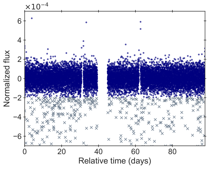
As seen in Fig. 3, the time series of HR 7322 shows a substantial number of outliers below the average flux level. As the data were obtained a few months before the second reaction wheel of the spacecraft failed, we follow the same approach as Johnson et al. 2014 and ascribe these outliers to pointing jitter caused by the increased friction that eventually led to the reaction wheel failure. The power density spectrum (PDS; Fig. 4) used for further seismic analysis was constructed from a weighted least-squares sine-wave fitting, single-side calibrated, normalised according to Parseval’s theorem, and converted to power density by multiplying by the effective observing length obtained from the integral of the spectral window (Kjeldsen & Frandsen 1992).

The individual mode frequencies for HR 7322 were extracted from the power spectrum using the peak-bagging approach described in Lund et al. 2017. Fig. 4 shows the PDS with the frequency of the fitted modes indicated, and as seen here HR 7322 shows a departure from the regularity in the mode degree pattern around $780\text{\,}\mathrm{\SIUnitSymbolMicro Hz}$ with two dipole modes (green triangles) being between two radial modes (orange diamonds) instead of only a single dipole mode. First-guesses for the mode frequencies included in the peak-bagging were obtained from visual inspection of the PDS. We note that $l=1$ modes were treated in the same way as pure p-modes, but with amplitudes and linewidths decoupled from the $l=0$ modes.

The large frequency separation $\Delta\nu$ and the frequency of maximum power $\nu_{\text{max}}$ were estimated by running the cleaned time series through the automated analysis pipeline described in Huber et al. 2009; Huber et al. 2011, and they were determined to be $\Delta\nu=$53.92\pm\pm 0.20\text{\,}\mathrm{\SIUnitSymbolMicro Hz}$$ and $\nu_{\text{max}}=$960\pm\pm 15\text{\,}\mathrm{\SIUnitSymbolMicro Hz}$$. The value of $\nu_{\text{max}}$ is in agreement with a simple Lorentz fit to the amplitudes of the individual modes.

Takeda et al. 2005 measured the projected rotational velocity $V\sin i$ of HR 7322 using spectroscopy to be $3\text{\,}\mathrm{km}\text{\,}{\mathrm{s}}^{-1}$, indicating either a low rotation rate or a pole-on view. From the peak-bagging, no clear independent values can be obtained for the rotational splitting ($\nu_{s}$) or stellar inclination. However, a seismic equivalent for the projected rotational velocity can be derived from the projected rotational splitting $\nu_{s}\sin i$ and the modelled stellar radius as $V\sin i=2\pi R\nu_{s}\sin i$ (Lund et al. 2014). We find a value of $V\sin i=4.5\pm 1.8\,\rm km\,s^{-1}$, in agreement with the value from Takeda et al. 2005.

The Hertzsprung SONG 1-m telescope (Andersen et al. 2014; Grundahl et al. 2017) at Observatorio del Teide on Tenerife was used to obtain high-resolution ($R=90000$) échelle spectra of HR 7322 on March 13 and September 16, 2016. Extraction of spectra, flat fielding and wavelength calibration were carried out with the SONG data reduction pipeline. Individual spectra were combined in iraf after correction for Doppler shifts resulting in a spectrum in the ${\sim}4400$–$6900\text{\,}\mathrm{\textup{\AA}}$ region with a signal-to-noise ratio of $\textup{S}/\textup{N}{\sim}400$ at $6000\text{\,}\mathrm{\textup{\AA}}$. For this spectrum, equivalent widths of the spectral lines listed in Nissen 2015 were measured by Gaussian fitting to the line profiles.

The equivalent widths were analysed with marcs model atmospheres (Gustafsson et al. 2008) with the method described in Nissen et al. 2017 to obtain abundances of elements. As seen in Eq. 1, the frequency of maximum power is related to the surface gravity and the effective temperature $\nu_{\text{max}}\propto g/\sqrt{T_{\textup{eff}}}$. A logarithmic surface gravity of $\log g=3.95\pm 0.01$ was determined for HR 7322 by using the asteroseismic $\nu_{\text{max}}$ and the interferometric $T_{\textup{eff}}$ (see Table 5) and by adopting $\text{T}_{\text{eff},\odot}=$5772\text{\,}\mathrm{K}$$, $\log g_{\odot}=4.438$, and $\nu_{\text{max},\odot}=$3090\text{\,}\mathrm{\SIUnitSymbolMicro Hz}$$ for the Sun. Then, the spectroscopic $T_{\textup{eff}}$ was determined from the requirement that the same Fe abundance should be obtained from Fe i and Fe ii lines. In this connection, non-LTE corrections from Lind et al. 2012 were taken into account, which decreases $T_{\textup{eff}}$ by $50\text{\,}\mathrm{K}$ relative to the LTE value. The results are $T_{\textup{eff}}=$6313\pm\pm 35\text{\,}\mathrm{K}$$ and $[\text{Fe/H}]=-0.23\pm 0.04$. We assume that the systematic uncertainties are of the same order of magnitude as the statistical uncertainties and add these uncertainties in quadrature to get a combined uncertainty of $50\text{\,}\mathrm{K}$ and $0.06\text{\,}\mathrm{d}\mathrm{e}\mathrm{x}$ respectively. Comparing this effective temperature from spectroscopy with the effective temperature from interferometry, we see that they have an excellent agreement within ${\sim}0.4\sigma$. Using this spectroscopic $T_{\textup{eff}}$ value in the scaling relation does not change $\log g$ significantly, i.e. by only $0.003\text{\,}\mathrm{d}\mathrm{e}\mathrm{x}$. As the two temperatures agree, we choose to use the interferometric temperature in the following analysis.

In addition, the ratio between the abundance of alpha-capture elements (Mg, Si, Ca, and Ti) and Fe was determined to be $[\text{$\alpha$/Fe}]=0.06\pm 0.03$ showing that HR 7322 belongs to the population of low-$\alpha$ (thin disk) stars.

We know the limb-darkened angular diameter $\theta_{\mathrm{LD}}$ of HR 7322 and thus the linear radius of the star can be estimated from Eq. 5 using an estimate of the distance, which is usually determined directly from the parallax $\varpi$. The parallax for HR 7322 was measured by the ESA missions Hipparcos and Gaia (van Leeuwen 2007; Gaia Collaboration et al. 2016a; Gaia Collaboration et al. 2016b). The Hipparcos mission measured the parallax of HR 7322 to be $\varpi=$23.79\pm\pm 0.32\text{\,}\mathrm{m}\mathrm{a}\mathrm{s}$$, while the second data release for the Gaia mission (Gaia DR2) report the parallax of HR 7322 to be $\varpi=$23.74\pm\pm 0.04\text{\,}\mathrm{m}\mathrm{a}\mathrm{s}$$ (Gaia Collaboration et al. 2018). We assess the astrometric solution of HR 7322 from Gaia by computing a re-normalised unit weight error of $\textup{RUWE}=0.82$ (Gaia Collaboration 2018), which is surprisingly low for such a bright target owing primarily to the colour index $\textup{G}_{\textup{BP}}-\textup{G}_{\textup{RP}}=0.637$ and the number of good observations ($\textup{n}_{\textup{good}}=175$) for HR 7322. Due to the good quality of the Gaia five-parameter solution, we choose to rely on the Gaia DR2 data for this bright target and trust a distance derived using this parallax.

We use the distance estimated for HR 7322 by Bailer-Jones et al. 2018, who inferred geometric distances from all parallaxes in the Gaia DR2 catalogue by using a exponentially decreasing space density prior estimated from a model of the Milky Way. The model does not take stellar properties or reddening into account. A significant zero-point offset in Gaia DR2 have been confirmed using various sources (Arenou et al. 2018; Zinn et al. 2018, e.g.) in the sense that parallaxes from Gaia DR2 are too small. Bailer-Jones et al. 2018 take this account by incorporating the global parallax zero-point from Lindegren et al. 2018 into the posterior probability density function. Using the distance from Bailer-Jones et al. 2018 in Eq. 5 yields an interferometric radius of the star of $R=$2.00\pm\pm 0.03\text{\,}\mathrm{\text{R}_{\odot}}$$. An estimate of reddening of HR 7322 was found to be approximately zero using the three-dimensional dust map from Green et al. 2018 and it does thus not violate the assumption of no reddening in the distance computation. This is also consistent with HR 7322 being close to us at a distance of ${\sim}$43\text{\,}\mathrm{p}\mathrm{c}$$ and within the Local Bubble.

Assuming that HR 7322 is homologous to the Sun, the asteroseismic scaling relations Eqs. 1 & 2 are valid, and we can find the asteroseismic estimate using the direct method in Eq. 4. We use the same $\nu_{\text{max},\odot}$ as in Sec. 2.4 along with $\Delta\nu_{\textup{solar}}=$135.1\text{\,}\mathrm{\SIUnitSymbolMicro Hz}$$. We find the asteroseismic radius and mass of HR 7322 to be $R=$2.04\pm\pm 0.04\text{\,}\mathrm{\text{R}_{\odot}}$$ and $M=$1.36\pm\pm 0.07\text{\,}\mathrm{\text{M}_{\odot}}$$ using the direct method.

However, the homology assumption leading to the scaling relation is not strictly valid. It has been shown that Eq. 4 holds within $5\text{\,}\mathrm{\,per\>cent}$ for dwarfs, subgiants, and giants (Stello et al. 2009; White et al. 2013; Huber et al. 2017, see e.g.) and that Eq. 3 holds within $10-$15\text{\,}\mathrm{\,per\>cent}$$ (Miglio 2012; Chaplin et al. 2014, see e.g.).

Previous studies have found that the scaling relations for $\Delta\nu$ and $\nu_{\text{max}}$ can be improved using corrections, typically written as a correction factor $f_{{\nu}_{\text{max}}}$ and $f_{\Delta\nu}$ multiplied on the right hand side of Eqs. 1 & 2 respectively. We still do not have a complete physical understanding of $\nu_{\text{max}}$, which also means that determining $f_{{\nu}_{\text{max}}}$ is an unresolved issue. Belkacem et al. 2011 proposed a dependence on the Mach number and mixing length parameter in the near-surface layers, meaning that $\nu_{\text{max}}$ should depend heavily on the physical conditions near the surface of the star. Viani et al. 2017 find that the most visible deviation between the observations and stellar models can be explained by adding a dependency on the mean molecular weight, however it seems that $[\text{Fe/H}]$ of HR 7322 is within the metallicity range where this additional term has little-to-no influence. White et al. 2011 studied a grid of stellar models and suggested a second-order polynomial correction to the $\Delta\nu$ scaling relation (Eq. 2) where $f_{\Delta\nu}$ is a function of the effective temperature. Sharma et al. 2016 suggested a correction depending on the evolutionary state, $[\text{Fe/H}]$, $\log g$, and $T_{\textup{eff}}$, where $f_{\Delta\nu}$ is found by interpolation in a grid based on stellar modelling. Sahlholdt et al. 2018 studied about $100$ main-sequence stars from the Kepler LEGACY sample (Lund et al. 2017; Silva Aguirre et al. 2017) and the Kages sample (Davies et al. 2016; Silva Aguirre et al. 2015) and found a linear and a quadratic polynomial parametrisation of $f_{\Delta\nu}$ and $f_{{\nu}_{\text{max}}}$ respectively, both only depending on the effective temperature.

A different approach is to derive new scaling relations with different exponents than in Eqs. 3 & 4. Bellinger 2019 derive new scaling relations not only for radius and mass but for stellar age as well, based on the same sample of main-sequence stars as Sahlholdt et al. 2018. In contrast to Sahlholdt et al. 2018, these scaling relations for mass and radius depend not only on effective temperature, but also contain a small, but non-zero dependency on metallicity as well. Kallinger et al. 2018 derive new non-linear scaling relation based on six red giants in eclipsing binary system along with about 60 red giants in the two open clusters NGC 6791 and NGC 6819 and as their correction is purely empirical, they do not contain any model-based correction terms.

In Table 3, the radius and mass of HR 7322 are calculated using these corrections, and we see that the different versions of the asteroseismic scaling relation for radius have a maximum ${\sim}0.8\sigma$ difference from the interferometric radius and are thus all in good agreement with the radius from interferometry.

We determine stellar properties of HR 7322 using grid-based stellar modelling. We construct grids of theoretical models of stellar evolution covering the necessary parameter space, which we compare the observed parameters to the predicted theoretical quantities. Quantities like stellar age can thus be estimated from the fit to the other observables. In this case, we fit the observed individual frequencies of HR 7322 along with the spectroscopic metallicity and the interferometric temperature to the grid.

Grids of stellar models were computed with the Garching Stellar Evolution Code (Weiss & Schlattl 2008, garstec;). The stellar models are computed using the Grevesse & Sauval 1998 solar mixture along with the OPAL equation of state (Rogers & Nayfonov 2002) and OPAL opacities (Iglesias & Rogers 1996) at high temperatures supplemented by the opacities of Ferguson et al. 2005 at low temperatures. garstec uses the NACRE nuclear reaction rates (Angulo et al. 1999) except for ¹⁴N($p,\gamma$)¹⁵O and ¹²C($\alpha,\gamma$)¹⁶O for which the rates from Formicola et al. 2004 and Hammer et al. 2005 were used. Convection was treated using the mixing-length formalism (Kippenhahn et al. 2012), where the fixed mixing length parameter was set to a solar-calibrated value of $\alpha_{\textup{mlt}}=1.818$. In the modelling of HR 7322, we used an Eddington grey atmosphere. Diffusion and settling of helium and heavier elements were not included, neither was convective overshooting. The stellar grid samples masses from $1.0$–$1.5$ $\mathrm{\text{M}_{\odot}}$ in steps of $0.01\text{\,}\mathrm{\text{M}_{\odot}}$ and it samples metallicities from $[\text{Me/H}]=-0.32$ to $-0.14$ in steps of $0.03$, assuming a fixed linear Galactic chemical evolution model of $\Delta Y/\Delta Z=1.4$ (Balser 2006). The grid covers $\Delta\nu$ in the range $50$–$60$ $\mathrm{\SIUnitSymbolMicro Hz}$, thus spanning the parameter space from about $5\text{\,}\mathrm{\SIUnitSymbolMicro Hz}$ on both sides of the observed $\Delta\nu$. The frequencies of the stellar models were computed using the Aarhus adiabatic pulsation code (Christensen-Dalsgaard 2008, adipls;). In order to correct for the systematic difference between the observed and the calculated frequencies introduced by the erroneous treatment of the near-surface layer in current stellar models, the two-term surface correction from Ball & Gizon 2014 was applied to the computed frequencies.

Three additional grids of stellar models were made in the same manner as described above (which we nickname nor): one with a lower mixing length parameter of $\alpha_{\textup{mlt}}=1.6$ (lowmlt), one with a higher mixing length parameter of $\alpha_{\textup{mlt}}=2.0$ (highmlt), and one including exponential convective overshooting with an efficiency parameter of $f=0.016$ (ove) (Freytag et al. 1996; Weiss & Schlattl 2008).

We use the BAyesian STellar Algorithm (Silva Aguirre et al. 2015; Silva Aguirre et al. 2017, basta;) to determine the stellar parameters of HR 7322. Given a precomputed grid of stellar models, basta uses a Bayesian approach to compute the probability density function of a given stellar parameter using a set of observational constraints. basta allows the possibility to add prior knowledge to the Bayesian fit, and we used the Salpeter Initial Mass Function (Salpeter 1955) as a prior to quantify our expectation of most stars being low-mass stars.

Including the frequencies in the fit has been done for other subgiant stars such as $\eta$ Boo (Kjeldsen et al. 1995; Christensen-Dalsgaard et al. 1995; Carrier et al. 2005), $\beta$ Hyi (Bedding et al. 2007; Brandão et al. 2011), and more recently $\mu$ Her (Grundahl et al. 2017; Li et al. 2019) and TOI 197 (Huber et al. 2019). As mentioned in Sec. 1, the observed p-modes in main-sequence stars are approximately evenly spaced in frequency. However, post-main-sequence stars do show deviations from this regularity as mode bumping occur due to a coupling between the acoustic p-modes in the expanding convective envelope and the buoyancy-driven g-modes in the stellar core (Osaki 1975; Aizenman et al. 1977). This coupling causes a range of non-radial pulsation modes to get mixed character – behaving like p-modes in the envelope and like g-modes in the core – which shifts the mode frequencies from their regular spacing and makes them stand out in the échelle diagrams as an avoided crossing.

In the échelle diagram of HR 7322 (Fig. 5), one dipole ($l=1$) avoided crossing is clearly visible. Fig. 6 shows how powerful avoided crossings can be to estimate precise stellar age. For a given mass and metallicity, only a few models spanning a narrow range in age of approximately $30$ Myr have the avoided crossing in-between the radial modes of radial order $n=13$ and $n=14$. When this is expanded to include the other masses and metallicities of the grid, the age range spans only about $100$ Myr, underlining how fitting this signature affects the uncertainty in age by constraining the parameter space much more than the spectroscopic values or the global asteroseimic parameters. This allows precise determination of stellar parameters (Deheuvels & Michel 2011; Benomar et al. 2014, see e.g.) and makes it possible to measure the age of the star with a relative statistical uncertainty of a few per cent (Metcalfe et al. 2010; Tian et al. 2015).

The results extracted from the probability density functions for each grid when fitting metallicity, interferometric temperature, and individual frequencies are seen in Table 4. The metallicity of HR 7322 was computed using the spectroscopic $[\text{Fe/H}]$ and [$\text{$\alpha$/Fe}]$ following Salaris et al. 2002. We compared the frequencies of the model in each grid with the lowest $\chi^{2}$ value to the observed oscillation frequencies. All four best-fitting models make very reasonable fits to the individual frequencies, but the set of frequencies from the best-fitting model in the lowmlt grid was the best match. An échelle diagram of the observed frequencies and the modelled frequencies from the best-fitting model from the lowmlt grid is seen in Fig. 5. We note that the model reproduces the clear dipole avoided crossing near $780\text{\,}\mathrm{\SIUnitSymbolMicro Hz}$ along with the two lower $l=1$ modes, which also seem to be mixed. There seems to be a frequency bump near $1200\text{\,}\mathrm{\SIUnitSymbolMicro Hz}$ that is present both in the $l=1$ and $l=2$ modes, which the modelled frequencies do not reproduce. As this bump appears in a part of the power spectrum with a high signal-to-noise ratio, this could be a real physical signature. This bump can be a result of the mismatch between the helium glitch signature in the observed and modelled frequency pattern (Verma et al. 2017, see e.g.). A mismatch would be of the same magnitude as the observed difference of $\sim{}$$1\text{\,}\mathrm{\SIUnitSymbolMicro Hz}$ and it would not depend on the spherical degree $l$. The helium glitch signature is difficult to measure for subgiants because of the avoided crossings, and therefore we have not added the helium glitch signature as a constraint to the fit.

The result from the lowmlt grid best reproduces all the observational constraints. In particular, the effective temperature of the other grids disagree significantly with the observed effective temperatures, given in Table 5. This is an effect of the different mixing length parameter $\alpha_{\textup{mlt}}$ in the grids. A decrease in $\alpha_{\textup{mlt}}$ changes the behaviour of the evolutionary tracks in a similar way to a decrease in metallicity by shifting the tracks towards hotter temperatures. This can explain why the lowmlt grid with the sub-solar $\alpha_{\textup{mlt}}$ finds a solution with a temperature about $150\text{\,}\mathrm{K}$ lower than the nor and ove grids with a solar $\alpha_{\textup{mlt}}$ and about $300\text{\,}\mathrm{K}$ lower than the highmlt grid with a super-solar $\alpha_{\textup{mlt}}$.

The value of the mixing length parameter $\alpha_{\textup{mlt}}$ is known to vary across the H-R diagram (Trampedach et al. 2014; Magic et al. 2015; Mosumgaard et al. 2018). The stagger grid (Magic et al. 2015) predicts the mixing length parameter of HR 7322 based on the interferometric temperature, spectroscopic metallicity, and $\log g$ to be less than their solar-calibrated value by about $\Delta\alpha_{\textup{mlt}}=0.2$, in agreement with the $\alpha_{\textup{mlt}}$ in the favoured lowmlt grid.

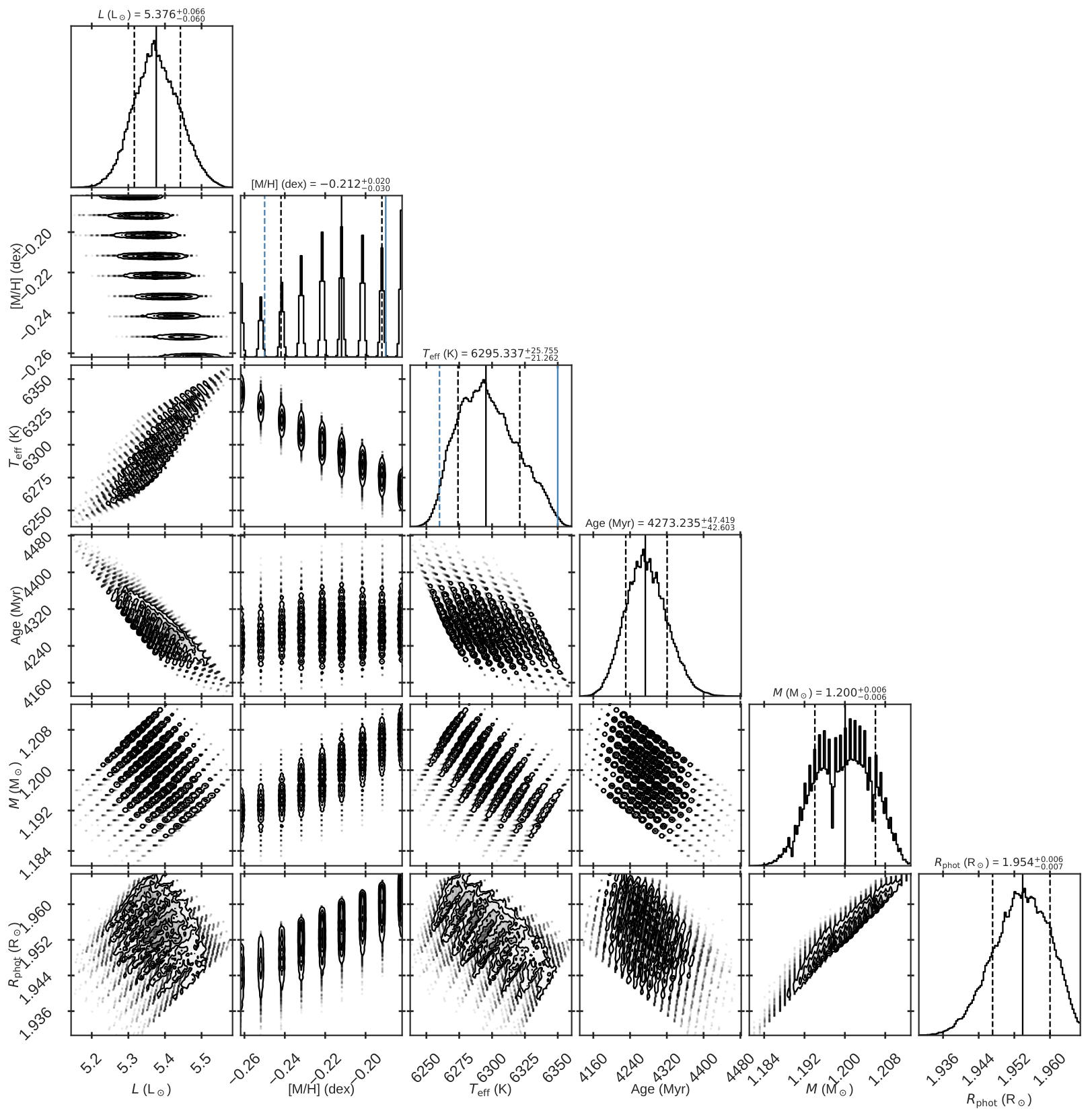
Observed individual frequencies constrain the parameter space considerably, narrowing down the formal uncertainties of the different parameters in the fit. In the case of mass and metallicity, we see in Table 4 that the uncertainties are equal to the resolution of the grid. In order to check if the uncertainties were physical or due to the limited grid resolution, we recomputed a finer grid with a higher resolution in mass $\Delta M=0.001$\mathrm{\text{M}_{\odot}}$$ and metallicity $\Delta[\text{Fe/H}]=0.01$. The results from this higher resolution grid can be seen in Table 5, and a plot of the probability density functions of the refined lowmlt grid can be seen in Fig. 9 in appendix. Interestingly, the solution only changed marginally and the uncertainties are at the same order of magnitude as in the results from the coarser version of the grid, showing that these narrow statistical uncertainties are due to the constrained parameter space and not due to the resolution of the grids.

In Fig. 7, we see the results of fitting different sets of parameters to this refined lowmlt grid. We see that by supplementing spectroscopic parameters with asteroseismic ones, we narrow down the uncertainties in particular in radius. However, we also see that none of the fits containing asteroseismic constraints reproduces the interferometric radius within 1 $\sigma$.

References

- Aerts et al. (2010) Aerts C., Christensen-Dalsgaard J., Kurtz D. W., 2010, Asteroseismology
- Aizenman et al. (1977) Aizenman M., Smeyers P., Weigert A., 1977, A&A, 58, 41
- Andersen et al. (2014) Andersen M. F., et al., 2014, in Revista Mexicana de Astronomia y Astrofisica Conference Series. p. 83
- Andrae et al. (2018) Andrae R., et al., 2018, A&A, 616, A8
- Angulo et al. (1999) Angulo C., et al., 1999, Nuclear Physics A, 656, 3
- Appourchaux & Grundahl (2013) Appourchaux T., Grundahl F., 2013, arXiv e-prints, p. arXiv:1312.6993
- Arenou et al. (2018) Arenou F., et al., 2018, A&A, 616, A17
- Bailer-Jones et al. (2018) Bailer-Jones C. A. L., Rybizki J., Fouesneau M., Mantelet G., Andrae R., 2018, AJ, 156, 58
- Ball & Gizon (2014) Ball W. H., Gizon L., 2014, A&A, 568, A123
- Balser (2006) Balser D. S., 2006, AJ, 132, 2326
- Basu & Chaplin (2017) Basu S., Chaplin W. J., 2017, Asteroseismic Data Analysis: Foundations and Techniques. Princeton University Press
- Bazot et al. (2011) Bazot M., et al., 2011, A&A, 526, L4
- Bedding et al. (2007) Bedding T. R., et al., 2007, ApJ, 663, 1315
- Belkacem et al. (2011) Belkacem K., Goupil M. J., Dupret M. A., Samadi R., Baudin F., Noels A., Mosser B., 2011, A&A, 530, A142
- Bellinger (2019) Bellinger E. P., 2019, arXiv e-prints,
- Benomar et al. (2014) Benomar O., et al., 2014, ApJ, 781, L29
- Bessell (2000) Bessell M. S., 2000, PASP, 112, 961
- Boyajian et al. (2009) Boyajian T. S., et al., 2009, ApJ, 691, 1243
- Boyajian et al. (2014) Boyajian T. S., van Belle G., von Braun K., 2014, AJ, 147, 47
- Brandão et al. (2011) Brandão I. M., et al., 2011, A&A, 527, A37
- Brown & Gilliland (1994) Brown T. M., Gilliland R. L., 1994, ARA&A, 32, 37
- Brown et al. (1991) Brown T. M., Gilliland R. L., Noyes R. W., Ramsey L. W., 1991, ApJ, 368, 599
- Campante (2018) Campante T. L., 2018, Asteroseismology and Exoplanets: Listening to the Stars and Searching for New Worlds, 49, 55
- Carrier et al. (2005) Carrier F., Eggenberger P., Bouchy F., 2005, A&A, 434, 1085
- Casagrande et al. (2011) Casagrande L., Schönrich R., Asplund M., Cassisi S., Ramírez I., Meléndez J., Bensby T., Feltzing S., 2011, A&A, 530, A138
- Chaplin & Miglio (2013) Chaplin W. J., Miglio A., 2013, Annual Review of Astronomy and Astrophysics, 51, 353
- Chaplin et al. (2014) Chaplin W. J., et al., 2014, ApJS, 210, 1
- Christensen-Dalsgaard (2008) Christensen-Dalsgaard J., 2008, Ap&SS, 316, 113
- Christensen-Dalsgaard et al. (1995) Christensen-Dalsgaard J., Bedding T. R., Houdek G., Kjeldsen H., Rosenthal C., Trampedach H., Monteiro M. J. P. F. G., Nordlund A., 1995, in Stobie R. S., Whitelock P. A., eds, Astronomical Society of the Pacific Conference Series Vol. 83, IAU Colloq. 155: Astrophysical Applications of Stellar Pulsation. p. 447 (arXiv:astro-ph/9503106)
- Code et al. (1976) Code A. D., Bless R. C., Davis J., Brown R. H., 1976, ApJ, 203, 417
- Davies et al. (2016) Davies G. R., et al., 2016, MNRAS, 456, 2183
- Deheuvels & Michel (2011) Deheuvels S., Michel E., 2011, A&A, 535, A91
- Deheuvels et al. (2016) Deheuvels S., Brandão I., Silva Aguirre V., Ballot J., Michel E., Cunha M. S., Lebreton Y., Appourchaux T., 2016, A&A, 589, A93
- Derekas et al. (2011) Derekas A., et al., 2011, Science, 332, 216
- Ferguson et al. (2005) Ferguson J. W., Alexander D. R., Allard F., Barman T., Bodnarik J. G., Hauschildt P. H., Heffner-Wong A., Tamanai A., 2005, ApJ, 623, 585
- Formicola et al. (2004) Formicola A., et al., 2004, Physics Letters B, 591, 61
- Freytag et al. (1996) Freytag B., Ludwig H. G., Steffen M., 1996, A&A, 313, 497
- Gaia Collaboration (2018) Gaia Collaboration ., 2018, Gaia Data Release 2 (DR2) gaia_source light, VO resource provided by the GAVO Data Center, http://dc.zah.uni-heidelberg.de/tableinfo/gaia.dr2light
- Gaia Collaboration et al. (2016a) Gaia Collaboration et al., 2016a, A&A, 595, A1
- Gaia Collaboration et al. (2016b) Gaia Collaboration et al., 2016b, A&A, 595, A2
- Gaia Collaboration et al. (2018) Gaia Collaboration et al., 2018, A&A, 616, A1
- García (2015) García R. A., 2015, in EAS Publications Series. pp 193–259 (arXiv:1510.02651), doi:10.1051/eas/1573004
- Gilliland et al. (2010) Gilliland R. L., et al., 2010, PASP, 122, 131
- Goldreich & Keeley (1977) Goldreich P., Keeley D. A., 1977, ApJ, 212, 243
- Green et al. (2015) Green G. M., et al., 2015, ApJ, 810, 25
- Green et al. (2018) Green G. M., et al., 2018, MNRAS, 478, 651
- Grevesse & Sauval (1998) Grevesse N., Sauval A. J., 1998, Space Sci. Rev., 85, 161
- Grundahl et al. (2017) Grundahl F., et al., 2017, ApJ, 836, 142
- Gustafsson et al. (2008) Gustafsson B., Edvardsson B., Eriksson K., Jørgensen U. G., Nordlund Å., Plez B., 2008, A&A, 486, 951
- Hammer et al. (2005) Hammer J. W., et al., 2005, Nuclear Phys. A, 758, 363
- Hanbury Brown et al. (1974) Hanbury Brown R., Davis J., Lake R. J. W., Thompson R. J., 1974, MNRAS, 167, 475
- Handberg & Lund (2014) Handberg R., Lund M. N., 2014, MNRAS, 445, 2698
- Hekker & Christensen-Dalsgaard (2017) Hekker S., Christensen-Dalsgaard J., 2017, A&ARv, 25, 1
- Høg et al. (2000) Høg E., et al., 2000, A&A, 355, L27
- Huber et al. (2009) Huber D., Stello D., Bedding T. R., Chaplin W. J., Arentoft T., Quirion P. O., Kjeldsen H., 2009, Communications in Asteroseismology, 160, 74
- Huber et al. (2011) Huber D., et al., 2011, ApJ, 743, 143
- Huber et al. (2012) Huber D., et al., 2012, ApJ, 760, 32
- Huber et al. (2017) Huber D., et al., 2017, ApJ, 844, 102
- Huber et al. (2019) Huber D., et al., 2019, arXiv e-prints, p. arXiv:1901.01643
- Iglesias & Rogers (1996) Iglesias C. A., Rogers F. J., 1996, ApJ, 464, 943
- Ireland et al. (2008) Ireland M. J., et al., 2008, in Optical and Infrared Interferometry. p. 701324, doi:10.1117/12.788386
- Johnson et al. (2014) Johnson J. A., et al., 2014, ApJ, 794, 15
- Jørgensen et al. (2017) Jørgensen A. C. S., Weiss A., Mosumgaard J. R., Silva Aguirre V., Sahlholdt C. L., 2017, MNRAS, 472, 3264
- Kallinger et al. (2010) Kallinger T., et al., 2010, A&A, 522, A1
- Kallinger et al. (2018) Kallinger T., Beck P. G., Stello D., Garcia R. A., 2018, A&A, 616, A104
- Kippenhahn et al. (2012) Kippenhahn R., Weigert A., Weiss A., 2012, Stellar Structure and Evolution, doi:10.1007/978-3-642-30304-3.
- Kjeldsen & Bedding (1995) Kjeldsen H., Bedding T. R., 1995, A&A, 293, 87
- Kjeldsen & Frandsen (1992) Kjeldsen H., Frandsen S., 1992, PASP, 104, 413
- Kjeldsen et al. (1995) Kjeldsen H., Bedding T. R., Viskum M., Frandsen S., 1995, AJ, 109, 1313
- Koch et al. (2010) Koch D. G., et al., 2010, ApJ, 713, L79
- Lebreton & Goupil (2014) Lebreton Y., Goupil M. J., 2014, A&A, 569, A21
- Li et al. (2019) Li T., Bedding T. R., Kjeldsen H., Stello D., Christensen-Dalsgaard J., Deng L., 2019, MNRAS, 483, 780
- Lind et al. (2012) Lind K., Bergemann M., Asplund M., 2012, MNRAS, 427, 50
- Lindegren et al. (2016) Lindegren L., et al., 2016, A&A, 595, A4
- Lindegren et al. (2018) Lindegren L., et al., 2018, A&A, 616, A2
- Lund et al. (2014) Lund M. N., et al., 2014, A&A, 570, A54
- Lund et al. (2017) Lund M. N., et al., 2017, ApJ, 835, 172
- Maestro et al. (2013) Maestro V., et al., 2013, MNRAS, 434, 1321
- Magic et al. (2015) Magic Z., Weiss A., Asplund M., 2015, A&A, 573, A89
- Mathur et al. (2012) Mathur S., et al., 2012, ApJ, 749, 152
- Metcalfe et al. (2010) Metcalfe T. S., et al., 2010, ApJ, 723, 1583
- Miglio (2012) Miglio A., 2012, Astrophysics and Space Science Proceedings, 26, 11
- Monnier (2003) Monnier J. D., 2003, Reports on Progress in Physics, 66, 789
- Mosumgaard et al. (2018) Mosumgaard J. R., Ball W. H., Silva Aguirre V., Weiss A., Christensen- Dalsgaard J., 2018, MNRAS, 478, 5650
- Neckel & Labs (1994) Neckel H., Labs D., 1994, Sol. Phys., 153, 91
- Nissen (2015) Nissen P. E., 2015, A&A, 579, A52
- Nissen et al. (2017) Nissen P. E., Silva Aguirre V., Christensen-Dalsgaard J., Collet R., Grundahl F., Slumstrup D., 2017, A&A, 608, A112
- O’Donnell (1994) O’Donnell J. E., 1994, ApJ, 422, 158
- Osaki (1975) Osaki J., 1975, Publications of the Astronomical Society of Japan, 27, 237
- Ricker et al. (2014) Ricker G. R., et al., 2014, in Space Telescopes and Instrumentation 2014: Optical, Infrared, and Millimeter Wave. p. 914320 (arXiv:1406.0151), doi:10.1117/12.2063489
- Rogers & Nayfonov (2002) Rogers F. J., Nayfonov A., 2002, ApJ, 576, 1064
- Sahlholdt et al. (2018) Sahlholdt C. L., Silva Aguirre V., Casagrande L., Mosumgaard J. R., Bojsen-Hansen M., 2018, MNRAS, 476, 1931
- Salaris et al. (2002) Salaris M., Cassisi S., Weiss A., 2002, Publications of the Astronomical Society of the Pacific, 114, 375
- Salpeter (1955) Salpeter E. E., 1955, ApJ, 121, 161
- Scherrer et al. (1983) Scherrer P. H., Wilcox J. M., Christensen-Dalsgaard J., Gough D. O., 1983. pp 75–87, doi:10.1007/BF00145547
- Sharma et al. (2016) Sharma S., Stello D., Bland-Hawthorn J., Huber D., Bedding T. R., 2016, ApJ, 822, 15
- Silva Aguirre et al. (2012) Silva Aguirre V., et al., 2012, ApJ, 757, 99
- Silva Aguirre et al. (2015) Silva Aguirre V., et al., 2015, MNRAS, 452, 2127
- Silva Aguirre et al. (2017) Silva Aguirre V., et al., 2017, ApJ, 835, 173
- Skrutskie et al. (2006) Skrutskie M. F., et al., 2006, AJ, 131, 1163
- Stello et al. (2009) Stello D., Chaplin W. J., Basu S., Elsworth Y., Bedding T. R., 2009, MNRAS, 400, L80
- Takeda et al. (2005) Takeda Y., et al., 2005, PASJ, 57, 13
- Tassoul (1980) Tassoul M., 1980, The Astrophysical Journal Supplement Series, 43, 469
- Tian et al. (2015) Tian Z., Bi S., Bedding T. R., Yang W., 2015, A&A, 580, A44
- Trampedach et al. (2014) Trampedach R., Stein R. F., Christensen-Dalsgaard J., Nordlund Å., Asplund M., 2014, MNRAS, 445, 4366
- Ulrich (1986) Ulrich R. K., 1986, ApJ, 306, L37
- Verma et al. (2014) Verma K., Antia H. M., Basu S., Mazumdar A., 2014, ApJ, 794, 114
- Verma et al. (2017) Verma K., Raodeo K., Antia H. M., Mazumdar A., Basu S., Lund M. N., Silva Aguirre V., 2017, ApJ, 837, 47
- Viani et al. (2017) Viani L. S., Basu S., Chaplin W. J., Davies G. R., Elsworth Y., 2017, ApJ, 843, 11
- Weiss & Schlattl (2008) Weiss A., Schlattl H., 2008, Ap&SS, 316, 99
- White et al. (2011) White T. R., Bedding T. R., Stello D., Christensen-Dalsgaard J., Huber D., Kjeldsen H., 2011, ApJ, 743, 161
- White et al. (2013) White T. R., et al., 2013, MNRAS, 433, 1262
- Zernike (1938) Zernike F., 1938, Physica, 5, 785
- Zinn et al. (2018) Zinn J. C., Pinsonneault M. H., Huber D., Stello D., 2018, arXiv e-prints, p. arXiv:1805.02650
- ten Brummelaar et al. (2005) ten Brummelaar T. A., et al., 2005, ApJ, 628, 453
- van Cittert (1934) van Cittert P. H., 1934, Physica, 1, 201
- van Leeuwen (2007) van Leeuwen F., 2007, A&A, 474, 653