Sparse Coding of Shape Trajectories for Facial Expression and Action Recognition
Abstract
The detection and tracking of human landmarks in video streams has gained in reliability partly due to the availability of affordable RGB-D sensors. The analysis of such time-varying geometric data is playing an important role in the automatic human behavior understanding. However, suitable shape representations as well as their temporal evolution, termed trajectories, often lie to nonlinear manifolds. This puts an additional constraint (i.e., nonlinearity) in using conventional Machine Learning techniques. As a solution, this paper accommodates the well-known Sparse Coding and Dictionary Learning approach to study time-varying shapes on the Kendall shape spaces of 2D and 3D landmarks. We illustrate effective coding of 3D skeletal sequences for action recognition and 2D facial landmark sequences for macro- and micro-expression recognition. To overcome the inherent nonlinearity of the shape spaces, intrinsic and extrinsic solutions were explored. As main results, shape trajectories give rise to more discriminative time-series with suitable computational properties, including sparsity and vector space structure. Extensive experiments conducted on commonly-used datasets demonstrate the competitiveness of the proposed approaches with respect to state-of-the-art.
Index Terms:
Kendall’s shape space, Shape trajectories, Sparse Coding and Dictionary Learning, Action recognition, Facial expression recognition.I Introduction
The availability of real-time skeletal data estimation solutions [Shotton11, cao2017realtime] and reliable facial landmarks detectors [xiong2013supervised, 6909636, baltrusaitis2018openface] has pushed researchers to study shapes of landmark configurations as well as their temporal evolution. For instance, 3D skeletons have been widely used to recognize human actions due to their ability in summarizing the human motion. Another example is given by the 2D facial landmarks and their tremendous use in facial expression analysis. However, human actions and facial expressions observed from visual sensors are often subject to view variations which makes their analysis complex. Considering this non-trivial problem, an efficient way to analyze these data takes into account view-invariance properties, giving rise to shape representations often lying to nonlinear shape spaces [kendall1984shape, bryner20142d, BenAmor:2016]. David G. Kendall [kendall1984shape] defines the shape as the geometric information that remains when location, scale, and rotational effects are filtered out from an object. Accordingly, one can represent 2D landmark faces and 3D skeletons as points in the 2D and 3D Kendall’s spaces, respectively. Further, when considering the dynamics of these points, the corresponding representations become trajectories in these spaces [BenAmor:2016]. However, inferencing such a representation remains challenging due to the nonlinearity of the underlying manifolds. In the literature, two alternatives have been proposed to overcome this problem for different Riemannian manifolds – they are either Extrinsic (kernel-based) [harandi2015extrinsic, DBLP:journals/corr/abs-1304-4344, jayasumana2013framework, 6751309] or Intrinsic [cetingul2009intrinsic, cetingul2011sparse, ho2013nonlinear, huang2016deep]. On one hand, extrinsic solutions are based on embeddings to higher dimensional Reproducing Kernel Hilbert Spaces (RKHS), which are vector spaces where Euclidean geometry applies. These methods bring the advantage that, as evidenced by kernel methods on , embedding a lower dimensional space in a higher dimensional one gives a richer representation of the data and helps capturing complex patterns. Nevertheless, to define a valid RKHS, the kernel function must be positive definite according to Mercer’s theorem [973]. Several works in the literature have studied kernels on the 2D Kendall’s space. For instance, the Procrustes Gaussian kernel is proposed in [jayasumana2013framework] as positive definite. In contrast, to our knowledge, such a kernel has not been explored for the 3D Kendall’s space. On the other hand, intrinsic solutions tend to project the manifold-valued data to a common tangent space attached to the manifold at a reference point [anirudh2015elastic, BenAmor:2016, Chellappa-CVPR-2014]. While it solves the problem of nonlinearity of the manifold of interest, this solution could introduce distortions, especially when the projected points are far from the reference point. In this work, we propose an extrinsic solution to represent 2D facial trajectories in RKHS and an intrinsic solution to model 3D actions. The latter brings a solution to the problem of distortions caused by tangent space approximations. In addition, we propose a comparative study of intrinsic and extrinsic solutions in the 2D and 3D Kendall’s spaces.
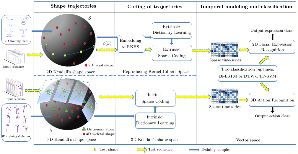
Motivated by the success of sparse representations in several recognition tasks [7565529, harandi2015extrinsic, ho2013nonlinear], we propose to code shape trajectories using Riemannian sparse coding and dictionary learning (SCDL). Specifically, 2D facial trajectories are coded in RKHS while sparse coding of 3D skeletal trajectories is performed in an intrinsic manner. As a main result, these coding techniques give rise to sparse times-series lying in vector spaces. In the contexts of facial expression recognition and action recognition, this brings two main advantages: (1) Sparse coding of shapes is performed with respect to a Riemannian dictionary. Hence, the resulting sparse times-series are expected to be more discriminative than the data themselves. In addition, they are robust to noise, knowing that SCDL is a powerful denoising tool; (2) Using sparse time-series as discriminative features allows us to perform both temporal modeling and classification in vector space, avoiding the more difficult task of classification on the manifold. An overview of the proposed approaches is given in Figure 1.
A preliminary version of this work appeared in [tanfous2018coding] with an application of intrinsic SCDL in the 3D Kendall’s space to model and recognize human actions. In this paper, we generalize the latter work to model and classify 2D facial expressions (micro and macro) in the 2D Kendall’s space. Moreover, we will provide a comparative study between the intrinsic and extrinsic approaches in the underlying shape spaces. This will be supported by extensive experiments and discussions. In summary, the main contributions of this work are,
- •
A novel human action and facial expression modeling based on SCDL in Kendall shape spaces. This allows to represent shape trajectories as time-series with suitable computational properties including sparsity and vector space structure.
- •
A comparative study of intrinsic and extrinsic SCDL solutions in the 2D and 3D Kendall’s spaces. To the best of our knowledge, this work is the first to apply both approaches to dynamic 2D and 3D shape related data.
- •
Application of our framework to 3D action recognition, 2D micro- and 2D macro- facial expression recognition. Extensive experiments are conducted on seven commonly-used datasets to show the competitiveness of the proposed approach to state-of-the-art.
The rest of the paper is organized as follows. In section II, we briefly review existing solutions of SCDL in nonlinear manifolds, geometric approaches in 3D action recognition, and some existing methods for 2D macro and micro facial expression recognition. Section III presents the geometry of the Kendall’s spaces, in addition to an embedding to RKHS that will be used to define the extrinsic SCDL solution. In section IV, we present the intrinsic and extrinsic frameworks of Riemannian SCDL. In section V, we describe the adopted temporal modeling and classification pipelines. Experimental results and discussions are reported in section VI, and section concludes the paper and draws some perspectives.
II Prior Work
In this section, we first focus our review on the extension of SCDL to nonlinear Riemannian manifolds. Then, we review geometric methods of 3D action recognition and 2D facial expression recognition.
II-A SCDL on Riemannian manifolds
Sparse representations have proved to be successful in various computer vision tasks which explains the significant interest in the last decade [7565529, harandi2015extrinsic, ho2013nonlinear]. Based on a learned dictionary, each data point can be represented as a linear combination of a few dictionary elements (atoms), so that a squared Euclidean loss is minimized. This assumes that the data points as well as the dictionary atoms are defined in vector space (to allow speaking on linear combination). However, most suitable image features often lie to nonlinear manifolds [Lui:2012]. Thus, to sparsely code these data while exploiting the Riemannian geometry of manifolds, the classical problem of SCDL needs to be extended to its nonlinear counterpart. Previous works addressed this problem [7565529, 6479703, harandi2015extrinsic, 7299018, ho2013nonlinear, 6751309, 6619442]. For instance, a straightforward solution was proposed in [6479703, Yuan2010] by embedding the manifolds of interest into Euclidean space via a fixed tangent space at a reference point. However, this solution could generate distortions since on a tangent space, only distances to the reference point are equal to true geodesic distances. To overcome this problem, Ho et al. [ho2013nonlinear] proposed a general framework for SCDL in Riemannian manifolds by working on the tangent bundle. Here, each point is coded on its attached tangent space where the atoms are mapped. By doing so, only distances to the tangent point are needed. Their proposed dictionary learning method includes an iterative update of the atoms using a gradient descent approach along geodesics. This general solution essentially relies on mappings to tangent spaces using the logarithm map operator. Although it is well defined for several manifolds, analytic formulation of the logarithm map is not available or difficult to compute for others. Therefore, some studies [harandi2015extrinsic, 7299018, DBLP:journals/corr/abs-1304-4344, 6751309] proposed to embed the Riemannian manifold into RKHS which depends on the existence of positive definite kernels, according to Mercer’s theorem [973]. For some Riemannian manifolds, such kernels are not available in the literature which disables the extension of sparse coding to Hilbert spaces. Recently, Harandi et al. [harandi2015extrinsic] proposed to map the Grassmann manifold into the space of symmetric matrices to allow the extension of sparse coding to Grassmann manifolds. They also proposed kernelized versions of the latter approach to handle the nonlinearity of the data, similarly proposed in [harandi2016sparse] for Symmetric Positive Definite matrices. In [7299018], the authors generalized sparse coding to nonlinear manifolds based on positive definite kernels. Their method was applied on three different Riemannian manifolds: the Grassmann manifold, the SPD manifold, and the 2D Kendall’s shape space. In particular, kernel SCDL was applied in the latter manifold for the task of shape classification. This method will be further studied in our work in the context of 2D dynamic facial expression recognition.
II-B 2D Facial Expression Recognition
The problem of facial expression recognition has attracted a particular attention in the last decades due to its potential in a wide spectrum of areas. The task here is to recognize the basic emotions (e.g., anger, disgust, surprise, etc.) from facial videos. Early works tackled this problem by extracting hand-crafted features that combine motion and appearance from image sequences such as LBP-TOP [zhao2007dynamic] and 3D SIFT [Liu_2014_CVPR, scovanner20073]. More recent approaches exploited deep neural networks such as 3D CNNs [liu2014deeply] and RNNs [ebrahimi2015recurrent]. In [7410698], two neural network architectures were proposed for image videos (DTAN) and 2D facial landmark sequences (DTGN) which are combined (forming DTAGN) to predict final emotions. In particular, DTGN showed to be efficient by using only 2D landmark sequences, when applied seperately. Another geometric approach was proposed in [wang2013capturing] which introduced a unified probabilistic framework based on an interval temporal Bayesian network (ITBN) built from the movements of landmark points. Aware of the small variations along a facial expression, the authors in [jain2011facial] proposed a method to capture the subtle motions within facial expressions using a variant of Conditional Random Fields (CRFs) called Latent-Dynamic CRFs (LDCRFs) on geometric features. Taking another direction, a method in [taheri2011towards] was proposed to represent 2D facial sequences as parametrized trajectories on the Grassmann manifold of 2-dimensional subspaces in ( is the number of landmarks) which is an affine-invariant shape representation. To capture the facial deformations, they used geodesic velocities between facial shapes and finally, classification was performed by applying LDA then SVM. In another work [Kacem_2017_ICCV], 2D facial landmark sequences were first represented as trajectories of Gram matrices in the manifold of positive semidefinite matrices of rank . A similarity measure is then provided by temporally aligning trajectories while taking into account the geometry of the manifold. This measure is finally used to train a pairwise proximity function SVM.
Although the macro facial expression recognition problem has seen considerable advances, micro-expression recognition is still a relatively challenging task [oh2018survey]. Micro-expressions are brief facial movements characterized by short duration, involuntariness and subtle intensity. In the literature, previous methods opted for extracting hand-crafted features from texture videos such as LBP-TOP and HOOF [zheng2016relaxed]. More recently, deep learning methods were proposed to tackle the problem by applying CNNs [breuer2017deep, kim2016micro] and RNNs [kim2016micro]. To our knowledge, only the method of [choi2018recognizing] is entirely based on analyzing 2D facial landmark sequences. Their work is based on computing the point-wise distances between adjacent landmark configurations along a sequence which is stacked in a matrix. The latter was seen as an input image to a CNN-LSTM-based classifier. However, their approach was only evaluated on a synthesized dataset produced from a macro-expression dataset. In our work, we will show that we achieve state-of-the-art results on a commonly-used micro-expression dataset using only 2D landmark data.
II-C Human Action Recognition from 3D skeletal data
Several approaches in the literature proposed spatio-temporal models to classify 3D action sequences. Early works extracted hand-crafted descriptors from 3D skeletal data. Popular examples include Key-Pose based descriptors [xia2012view, ofli2014sequence] and dynamics-based descriptors [zanfir2013moving, chaudhry2013bio]. More recently, deep learning was applied to recognize 3D actions. Both feed-forward neural networks such as CNNs [ke2017new, kim2017interpretable, yan2018spatial] and several variants of recurrent neural networks such as LSTM [liu2016spatio, zhu2016co, zhang2017view] were proposed. The above-mentioned approaches did not make any manifold assumptions on the data representation. However, several shape representations and their dynamics often lie to nonlinear manifolds. As a consequence, many approaches exploited the Riemannian geometry of nonlinear manifolds to analyze skeletal sequences. For instance, in [Chellappa-CVPR-2014], the authors proposed to represent skeletal motion as trajectories in the Special Euclidean (Lie) group (respectively ). These representations are then mapped into the correspondent Lie algebra (respectively ) which is a vector space, the tangent space attached to the Lie group at the identity, where they are processed and classified. Exploiting the same representation on Lie Groups, the authors in [anirudh2015elastic] used the framework of Transported Square-Root Velocity Fields (TSRVF) [su:AOAS:2013] to encode trajectories lying on Lie groups. They extended existing coding methods such as PCA, KSVD, and Label Consistent KSVD to these Riemannian trajectories. Another approach [BenAmor:2016] proposed a different solution by extending the Kendall’s shape theory to trajectories. Accordingly, translation, rotation, and global scaling are first filtered out from each skeleton to quantify the shape. Then, based on the TSRVF, they defined an elastic metric to jointly align and compare trajectories. Here, trajectories are transported to a reference tangent space attached to the Kendall’s shape space at a reference point. A common major drawback of these approaches is mapping trajectories to a reference tangent space which may introduce distortions. Conscious of this limitation, the authors in [vemulapalli2016rolling] proposed a mapping of trajectories on Lie groups combining the usual logarithm map with a rolling map that guarantees a better flattening of trajectories on Lie groups. In our work, we represent skeletal sequences as trajectories in the Kendall’s shape space and to overcome its nonlinearity, we propose to code them with an intrinsic formulation of SCDL that avoids distortions caused by tangent space approximations.
III Preliminaries
In the following, we review the geometry of the Kendall’s space in the case of 2D planar shapes and 3D skeletal data. Then, we describe the embedding of 2D shapes to RKHS.
III-A Geometry of the Kendall’s shape space
Let us consider a set of landmarks in (). To represent its shape, Kendall [kendall1984shape] proposed to establish equivalences with respect to shape-preserving transformations that are translations, rotations, and global scaling. Let represent a configuration of landmarks. To remove the translation variability, we follow [dryden-mardia] and introduce the notion of Helmert sub-matrix, a sub-matrix of a commonly used Helmert matrix, to perform centering of configurations. For any , the product represents the Euclidean coordinates of the centered configuration. Let be the set of all such centered configurations of landmarks in , i.e., . is a dimensional vector space and can be identified with . To remove the scale variability, we define the pre-shape space to be: ; is a unit sphere in and, thus, is dimensional. The tangent space at any pre-shape is given by: . To remove the rotation variability, for any , we define an equivalence class: that represents all rotations of a configuration . The set of all such equivalence classes, is called the shape space of configurations. The tangent space at any shape is , where is any skew-symmetric matrix. The first condition makes tangent to and the second makes perpendicular to the rotation orbit. Together, they force to be tangent to the shape space . Assuming standard Riemannian metric on , the geodesic between two points is defined as:
| (1) |
where , is the inner product on , and is the optimal rotation that aligns with : . This is also the geodesic distance between and in the shape space , representing the optimal deformation to connect to in . For , and for we have . The mapping of a point to the tangent space attached at is done by the logarithm map operator:
| (2) |
The inverse operation, e.g., exponential map, applies the shooting vector to a source shape and provides the deformed (target) shape. It is defined, for any , by,
| (3) |
Note that Kendall’s shape space is a complete Riemannian manifold such that the logarithm map is defined for all . As a consequence, the geodesic distance between two configurations and can be computed as , where denotes the norm induced by the Riemannian metric at .
The case of planar shapes – For , a 2D landmark configuration can be initially represented as a -dimensional complex vector whose real and imaginary parts respectively encode the and coordinates of the landmarks. In this case, the pre-shape space is defined, after removing the translation and scale effects, as: ; is a complex unit sphere of dimension . The rotation removal consists of defining, for any , an equivalence class that represents all rotations of a configuration . The final shape space is the set of all such equivalence classes . To measure the distance between two shapes and , we define the most popular distance on the 2D Kendall’s shape space, named the full Procrustes Distance [kendall1984shape], as
| (4) |
where and denote the inner product in and the absolute value of a complex number, respectively.
III-B Embedding of 2D shapes into RKHS
A Hilbert space is a high (often infinite) dimensional vector space that possesses the structure of an inner product allowing to measure angles and distances. To define an inner product in , we will use a kernel function which makes the resulting space a RKHS. The embedding of Kendall’s space to RKHS brings the main advantage of transforming the nonlinear manifold into a vector space where one can directly apply algorithms designed for linear data. In addition, it gives a richer representation of the original data in a higher-dimensional space. This is beneficial for the specific task of SCDL which essentially relies on measures of similarities, i.e., on an inner product. However, to define a valid RKHS, the kernel function must be positive definite, according to Mercer’s theorem [973]. For the Kendall’s space of 2D shapes, the authors of [jayasumana2013framework] have proved the positive definiteness of the Procrustes Gaussian kernel which is defined as
| (5) |
where is the full Procrustes Distance defined in Eq.(4). This kernel is positive definite for all . In the following section, it will be used to extend SCDL to RKHS.
IV Riemannian coding of shapes
Before presenting the two Riemannian SCDL solutions, i.e., intrinsic and extrinsic, we start by recalling the classic formulation of SCDL in Euclidean space. Let be a set of vectors in denoting a dictionary of atoms, and a query data point. The problem of sparse coding with respect to can be expressed as
| (6) |
where denotes the vector of codes comprised of , is the sparsity inducing function defined as the norm, and is the sparsity regularization parameter. Eq. 6 seeks to optimally approximate (by ) as a linear combination of atoms, i.e., , while tacking into account a particular sparsity constraint on the codes, . This sparsity function has the role of forcing to be represented as only a small number of atoms.
Given a finite set of training observations in , learning a Euclidean dictionary is defined as to jointly minimize the coding cost over all choices of atoms and codes according to:
| (7) |
To solve this non-convex problem, a common approach alternates between the two sets of variables, and , such that: (1) Minimizing over while is fixed is a convex problem (i.e., sparse coding). (2) Minimizing Eq. 7 over while is fixed is similarly a convex problem.
IV-A Extrinsic approach
The SCDL algorithms depend on the notion of inner product. In the following, we will discuss how it can be easily extended to RKHS.
IV-A1 Extrinsic Sparse Coding
A closed-form solution of extrinsic sparse coding is proposed in [harandi2015extrinsic]. To derive it, let us first define a mapping to RKHS induced by the kernel , where . For a query shape , extending Eq. 6 to RKHS yields
| (8) |
with . In Eq. 8, since the sparsity term depends entirely on , only the reconstruction term needs to be kernelized. Expanding the latter gives
| (9) |
where is the -dimensional kernel vector computed between the query and the dictionary atoms, and is the kernel matrix computed between the atoms. An efficient solution of kernel sparse coding can be obtained by considering as the SVD of the symmetric positive definite kernel , and as a constant term (independent on ). Thus, Eq. 9 can be written as the least-squares problem in : , where and (we refer to [harandi2015extrinsic] for the proof). In this work, this approach is applied in the Kendall’s shape space by using the kernel defined in subsection III-B.
IV-A2 Extrinsic Dictionary learning
Similarly to Euclidean dictionary learning, the extrinsic Riemannian formulation is based on an alternating optimization strategy to update weights and atoms. While the first step is obtained with extrinsic sparse coding presented above, the second is presented in what follows. Given the codes from the first step, the problem of dictionary learning can be viewed as optimizing Eq. 8 over . The main idea here is to represent as a linear combination of the training samples in RKHS, according to the Representer theorem [Schlkopf2001AGR]. The resulting weights for the training samples are stacked in a matrix , which gives . Since only the first term in Eq. 8 depends on , the problem of dictionary update can be written as , where W is the matrix of sparse codes obtained from the first step. The latter can be expanded to
To obtain the updated dictionary that is now defined by , the gradient of is zeroed out w.r.t . This gives , where † is the pseudo-inverse operator.
IV-B Intrinsic approach
To deal with the nonlinearity of Kendall’s space, a common approach opted for projecting manifold-valued data to a tangent space at a reference point (e.g., the mean shape). However, such a projection only results in first-order approximation of the data. The latter can be distorted, especially if points are far from the tangent point. In what follows, we will show how this problem can be avoided in the intrinsic formulation of SCDL.
IV-B1 Intrinsic Sparse Coding
Let be a dictionary on , and similarly the query is a point on . Accordingly, the problem of sparse coding involves the geodesic distance defined on and, thus, becomes
| (10) |
Here, denotes an encoding function that generates the approximated point on by combining atoms with codes. Note that in the special case of Euclidean space, would be a linear combination of atoms. However, in the Riemannian manifold , we have forsaken the structure of vector space which makes the linear combination of atoms lying on no longer applicable, since the approximated may lie out of the manifold. An interesting alternative is the intrinsic formulation of Eq. 10, when considering that is a complete Riemannian manifold, thus, the geodesic distance (as explained in section III-A). As a consequence, the cost function in 10 can be written as
| (11) |
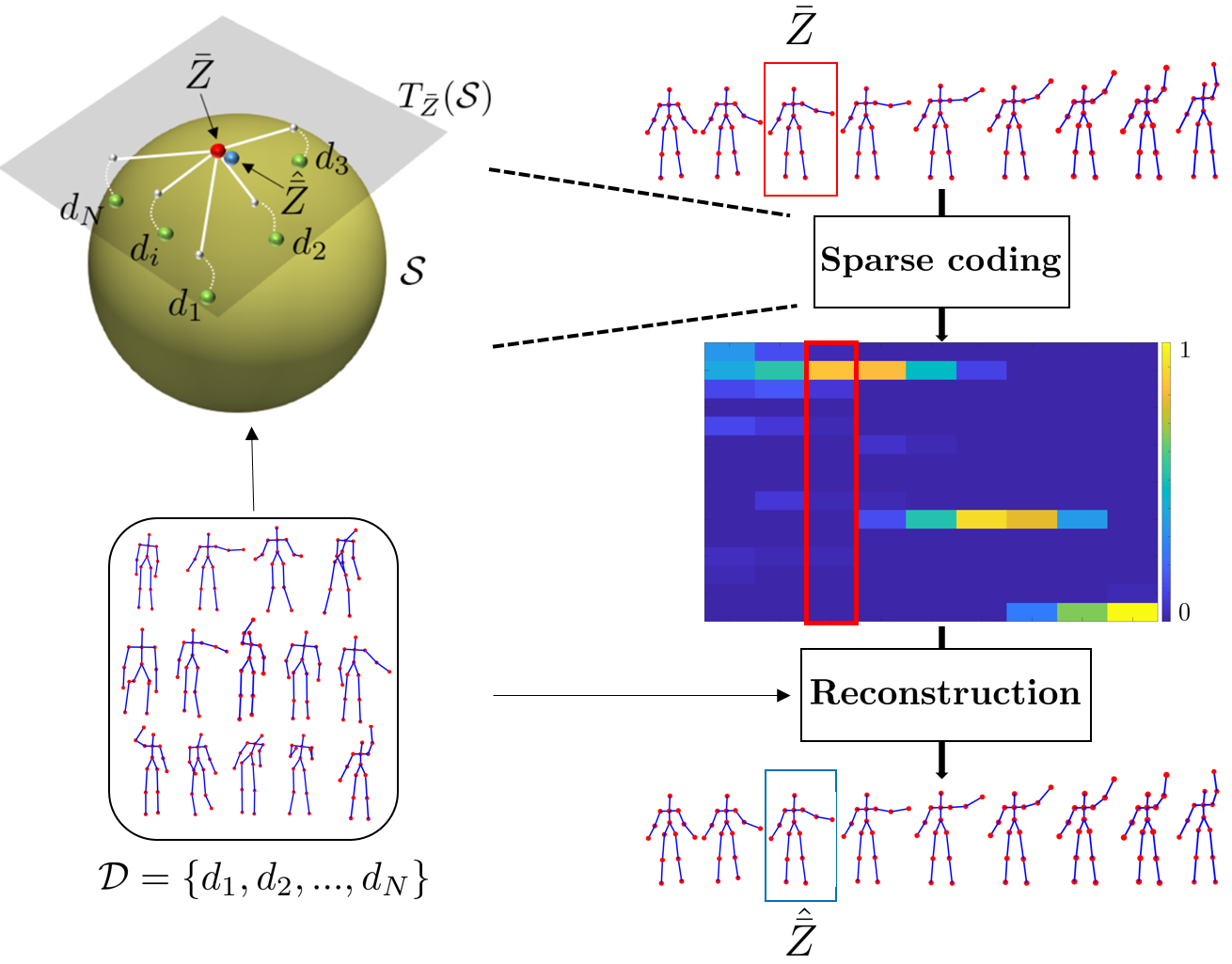
where denotes the logarithm map operator that maps each atom to the tangent space at the point being coded, and is the norm induced by the Riemannian metric at . Mathematically, this allows to partially compensate the lack of vector space structure on , as illustrated in Figure 2. To avoid the solution , we imposed in Eq. 11 an important additional affine constraint defined as . By this formulation of sparse coding, we only compute distances to the tangent point, hence we avoid the commonly induced distortions when working in a reference tangent space. By substituting the logarithm map by its explicit formulation in Eq. 11, we have
| (12) |
In practice, Eq. 12 is computed by first finding the optimal rotation between and each atom via the Procrustes algorithm [kendall1984shape]. Then, we solve for using the state-of-the-art CVXPY optimizer [cvxpy].
IV-B2 Intrinsic Dictionary Learning
Learning a discriminative dictionary typically yields accurate reconstruction of training samples and produces discriminative sparse codes. We propose a dictionary learning algorithm based on the sparse coding framework described above. Let be a dictionary on , and similarly is a set of training samples on . Similarly to the sparse coding problem, we introduce in Eq. 7 the geodesic distance defined on computed as . As a consequence, the problem of dictionary learning on Kendall’s shape space is written as
| (13) |
with the important affine constraint . Similar to the Euclidean case, the optimization problem can be solved by iteratively performing sparse coding while fixing , and optimizing while fixing the sparse codes.

IV-C Kernel clustering of shapes for dictionary learning
The performance of SCDL depends on the number of the dictionary elements , and an empiric choice of can be time consuming, especially when it comes to large datasets. As a solution, we propose an initialization step that enables an automatic inference on and accelerates the convergence of the dictionary learning algorithm. To this end, we propose to cluster the training shapes by adapting the Bayesian clustering of shapes of curves method proposed in [Zhang2015171]. In Figure 3, we show the main steps of the proposed clustering approach. First, an inner product matrix is computed from the training data based on the kernel function defined in subsection III-B. Note that in the 3D case, this kernel is positive definite for only certain values of the kernel parameter . Thus, its empiric choice is required to seek positive definiteness. The inner product matrix is then modeled using a Wishart distribution. To allow for an automatic inference on the number of clusters, prior distributions are carefully assigned to the parameters of the Wishart distribution. Then, posterior is sampled using a Markov chain Monte Carlo procedure based on the Chinese restaurant process for final clustering. We refer the reader to [Zhang2015171] for further details.
Dictionary initialization – Given a set of training samples on , the idea is to select representatives to initialize the dictionary. This is done in two main steps: (1) Clustering of shapes as described above; (2) Generating atoms from each cluster such that they well describe the intra-cluster variability. In the second step, for each cluster, we propose to perform principal geodesic analysis (PGA), first proposed by [fletcher2004principal], to obtain the best representatives of the cluster. Specifically, we map all cluster elements to the tangent space of the mean shape . Then, we perform principal component analysis (PCA) in this vector space. Finally, the resulting vectors from all the clusters are mapped to to represent the initial atoms of . Note that an advantage of performing PGA in each cluster rather than in the whole training set is to avoid the problematic case of having points in the manifold that are far from the tangent point.
V Temporal modeling and classification
Let be a sequence of landmark configuration representing a trajectory on . As described in section IV, we code each skeleton into a sparse vector of codes with respect to a dictionary ( is given a particular structure described later on in this section). As a consequence, each trajectory is mapped to a -dimensional function of sparse codes and the problem of classifying trajectories on is turned to classifying -dimensional sparse codes functions in Euclidean space, where any traditional operation on Euclidean time-series (e.g., standard machine learning techniques) could be directly applied. Several methods in the literature tend to process and classify time series [anirudh2015elastic, BenAmor:2016, Chellappa-CVPR-2014, vemulapalli2016rolling]. In our work, we adopt two different classification schemes to perform action and facial expression classification: (1) A pipeline of Dynamic Time Warping (DTW), Fourier Temporal Pyramid (FTP), and one-vs-all linear SVM. Thus, we handle rate variability, temporal misalignment and noise, and classify final features, respectively; (2) Bidirectional Long short-term memory (Bi-LSTM) which is an extension of the traditional LSTM that represents each sequence backwards and forwards to two separate recurrent networks, providing context from both the future and past [graves2005framewise].
Dictionary structure – In the context of classification, one may exploit the important information of data labels to construct more discriminative feature vectors. To this end, we propose to build class-specific dictionaries, similarly to [guha2012learning]. Formally, let be a set of labeled trajectories on belonging to different classes , we aim to build class-specific dictionaries in such that each is learned using skeletons belonging to training sequences from the corresponding class . In this scenario, coding a query skeletal shape is done with respect to each , independently. As a result, vectors of codes are obtained. These vectors are finally concatenated to form a global feature vector .
VI Experiments
To evaluate the proposed modeling approaches, we conducted extensive experiments on three applications: 2D macro facial expression recognition, 2D micro-expression recognition, and 3D action recognition. We further provide a comparative evaluation on the two SCDL frameworks that we used in the context of these applications.
Experimental Settings and Parameters – In all experiments, the values of the kernel parameter and the sparsity regularization parameter were chosen empirically. We classified the final time-series based on the two classification schemes presented in section V. In the first scheme, i.e., DTW-FTP-SVM, we used a six-level FTP and fixed the value of SVM parameter C to 1. In the second scheme, we train the network with one Bi-LSTM layer, with the exeption of NTU-RGB+D dataset where two layers were used. The minimization is performed using Adam optimizer and the applied probability of dropout is 0.3. The value of neuron size was chosen empirically for each dataset.
VI-A 2D Facial Expression Recognition
In this application, we extract 49 facial landmarks from human faces in 2D and with high accuracy using a state-of-the-art facial landmark detector [6909636]. We first represent the sequences of landmarks as trajectories in the Kendall’s shape space. Extrinsic SCDL is then applied to produce sparse time-series that are finally classified in vector space. We evaluate this approach on two different 2D facial expression recognition problems: the macro and micro.
VI-A1 Macro-Expression Recognition
The task here is to recognize the basic macro emotions, e.g., fear, surprise, happiness, etc. To this end, we applied our approach on two commonly-used datasets namely the Cohn-Kanade Extended dataset and the Oulu-CASIA dataset. Our obtained results are then discussed with respect to state-of-the-art approaches as well as to intrinsic SCDL. For both datasets, we followed the commonly-used experimental setting in [ELAIWAT2016152, 7410698, 6909622, 6247974] consisting on a 10-fold cross validation.
- •
Cohn-Kanade Extended (CK+) dataset [5543262] consists of 327 image sequences performed by 118 subjects with seven emotion labels: anger, contempt, disgust, fear, happiness, sadness, and surprise. Each sequence contains the two first temporal phases of the expression, i.e., neutral and onset (with apex frames).
- •
Oulu-CASIA dataset [article] includes 480 image sequences performed by 80 subjects. They are labeled with one of the six basic emotions (those in CK+, except the contempt). Each sequence begins with a neutral facial expression and ends with the expression apex.
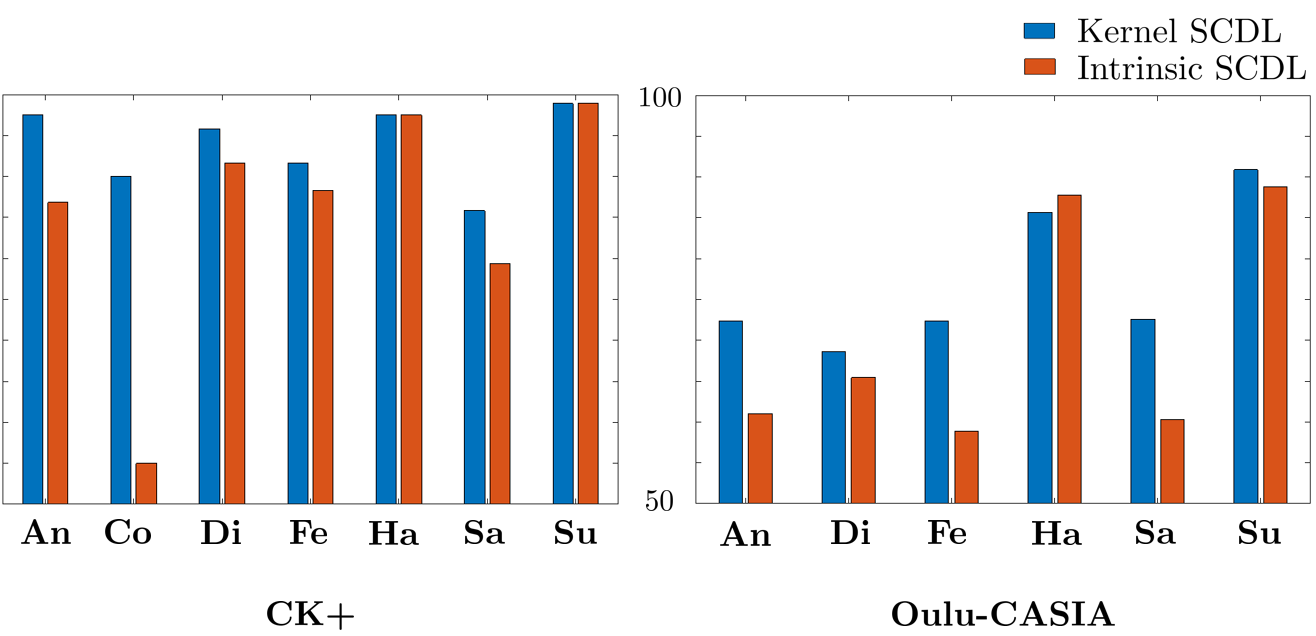
Results and discussions – Table I gives an overview of the obtained results on both datasets. Overall, our approach achieved competitive results compared to the literature. For instance, our best result on CK+ (obtained with Bi-LSTM) is by lower than the best state-of-the-art result obtained by the method of [7410698]. The latter is based on two neural network architectures trained on image videos and facial landmark sequences. However, when using only the landmark architecture (DTGN), our approach obtained a higher accuracy. Similarly, on Oulu-CASIA, our best result is lower than DTAGN and higher than DTGN. On the other hand, the method of [Kacem_2017_ICCV] achieved a better performance on both datasets compared to our method. Comparing the confusion matrices, the same method seems to better recognize the sadness expression while our method is clearly more efficient in recognizing the contempt expression. This will be further discussed later on. From Fig. 4 and the confusion matrix in Table VI-A1, we can observe that the two expressions: happiness and surprise are well recognized in the two datasets while the main confusions happened in the two expressions: fear and sadness, conforming to state-of-the-art results [Kacem_2017_ICCV, 7410698]. Besides, we highlight the superiority of extrinsic SCDL compared to intrinsic SCDL. The first is performed in RKHS which is a higher dimensional vector space. This helps capturing complex patterns in facial expressions and identifying subtle differences between similar expressions. For instance, an interesting observation could be seen for the contempt expression. As stated in [5543262], the latter is quite subtle and it gets easily confused with other, strong emotions. For this expression, the recognition accuracy obtained with intrinsic SCDL is , compared to obtained with extrinsic SCDL, as shown in Figure 4. We argue that this remarkable improvement comes from the mapping to RKHS for the same reasons mentioned above. This observation has pushed us to further evaluate the performance of our approach in the task of micro-expression recognition.
| Method | CK+ | Oulu-CASIA |
|---|---|---|
| (A) CSPL [6247974] | 89.89 | – |
| (A) ST-RBM [ELAIWAT2016152] | 95.66 | – |
| (A) STM-ExpLet [6909622] | 94.19 | 74.59 |
| (G) ITBN [wang2013capturing] | 86.30 | – |
| (G) DTGN [7410698] | 92.35 | 74.17 |
| (A+G) DTAGN [7410698] | 97.25 | 81.46 |
| (R)Shape velocity on Grassmannian [taheri2011towards] | 82.80 | – |
| (R)Shape traj. on Grassmannian [Kacem_2017_ICCV] | 94.25 | 80.0 |
| (R)Gram matrix trajectories [Kacem_2017_ICCV] | 96.87 | 83.13 |
| (R)Intrinsic SCDL (SVM) | 91.26 | 70.37 |
| (R)Intrinsic SCDL (Bi-LSTM) | 89.43 | 70.24 |
| (R)Extrinsic SCDL (SVM) | 95.62 | 77.06 |
| (R)Extrinsic SCDL (Bi-LSTM) | 95.73 | 73.09 |
| Predicted | |||||||
|
Angry |
Disgust |
Fear |
Happy |
Sadness |
Surprise | ||
| Actual | Angry | 72.33 | 12.33 | 2.11 | 1 | 12.22 | |