A probabilistic protocol for the assessment of transition and control
Abstract
Transition to turbulence dramatically alters the properties of fluid flows. In most canonical shear flows, the laminar flow is linearly stable and a finite-amplitude perturbation is necessary to trigger transition. Controlling transition to turbulence is achieved via the broadening or narrowing of the basin of attraction of the laminar flow. In this paper, a novel methodology to assess the robustness of the laminar flow and the efficiency of control strategies is introduced. It relies on the statistical sampling of the phase space neighborhood around the laminar flow in order to assess the transition probability of perturbations as a function of their energy. This approach is applied to a canonical flow (plane Couette flow) and provides invaluable insight: in the presence of the chosen control, transition is significantly suppressed whereas plausible scalar indicators of the nonlinear stability of the flow, such as the edge state energy, do not provide conclusive predictions. The methodology presented here in the context of transition to turbulence is applicable to any nonlinear system displaying finite-amplitude instability.
keywords
Authors should not enter keywords on the manuscript, as these must be chosen by the author during the online submission process and will then be added during the typesetting process (see http://journals.cambridge.org/data/relatedlink/jfm-keywords.pdf for the full list)1 Introduction
Controlling transition to turbulence is vitally important in a variety of applications ranging from pipeline flows to mixing devices. In the former, turbulence undesirably enhances transport losses, whilst in the latter, it improves mixing efficiency. A large body of research has been devoted to specific passive and active control strategies to decrease transport losses by reducing the friction drag of turbulent flows (Jung et al. 1992; Baron & Quadrio 1995; Quadrio & Ricco 2004; Kasagi et al. 2009; Quadrio 2011; Brunton & Noack 2015). Another ongoing effort to control transition is aimed at manipulating the robustness of the laminar flow to perturbations via passive modifications of channel surfaces and linear feedback control techniques (Sreenivasan 1982; Kim & Bewley 2007; Hof et al. 2010; Rabin et al. 2014; Marensi et al. 2019). The resulting strategies are largely based on the knowledge that, in subcritical shear flows, transition to long-lived turbulence occurs when both the Reynolds number, quantifying the ratio of the inertia of the flow to the viscous forces, exceeds a critical value (Avila et al. 2011; Shi et al. 2013), and a sufficiently energetic disturbance is applied (Schmiegel & Eckhardt 1997; Duguet et al. 2013). A strategy designed to prevent transition can be deemed successful when it increases the volume of the basin of attraction of the laminar flow relative to the state space volume. This relative volume is related to the edge of chaos, the manifold separating initial conditions that decay from those that transition (Skufca et al. 2006; Schneider et al. 2008; Chantry & Schneider 2014). The edge of chaos comprises local attractors, the edge states, and their stable manifolds. The importance of edge states has indeed been highlighted for boundary layer and pipe flows, where their neighborhood is often visited before transition (Mellibovsky et al. 2009; Khapko et al. 2016), and for plane Couette flow, where they have been related to optimal energy growth disturbances (Duguet et al. 2010; Olvera & Kerswell 2017) and utilized for controlling transition to turbulence (Kawahara 2005). The energy of the edge state, together with that of minimal seeds, i.e., that of the minimal energy perturbations that trigger turbulence (Pringle et al. 2012; Duguet et al. 2013), can therefore be thought of as main scalar indicators of the robustness of the laminar flow to finite amplitude perturbations.
A tempting way to design control strategies for transition is via the maximization of the energy of the minimal seed (Rabin et al. 2014) or of the edge state. In this paper, we show that such quantities may be insufficient to provide a reliable conclusion about the efficiency of control strategies. To address such shortcomings, we introduce a novel methodology: the statistical sampling of the phase space to determine the probability that perturbations laminarize as a function of their energy. We apply this approach in plane Couette flow where control is imposed via transverse wall oscillations (Jung et al. 1992; Baron & Quadrio 1995; Quadrio & Ricco 2004; Rabin et al. 2014).
2 Protocol
We consider plane Couette flow, i.e., the flow confined between two infinite plates separated by a gap and moving in opposite directions with constant velocity . The domain is periodic in the streamwise (period ) and in the spanwise (period ) directions, and no-slip boundary conditions are applied at the walls (Pershin et al. 2019). The nondimensionalized Navier–Stokes equation and the incompressibility condition are given by:
| (1) | |||
| (2) |
where is the Reynolds number, is the kinematic viscosity, is the pressure, is the unit vector in the streamwise direction and satisfies homogeneous boundary conditions in . To obtain these equations, we have decomposed the nondimensional velocity , where the laminar flow and is the incompressible perturbation. The no-slip boundary conditions read: .
We use Channelflow (Gibson 2014) to solve for the flow at various values of the Reynolds number , where is the critical value above which sustained turbulence can be observed (Shi et al. 2013; Dauchot & Daviaud 1995), and in the presence of control by wall oscillations at . The streamwise and spanwise coordinates are discretized using and Fourier coefficients and the wall-normal coordinate is discretized using Chebyshev coefficients based on the numerical resolution used in Pershin et al. 2019. The temporal discretization is performed by means of 3rd-order semi-implicit backward differentiation with time step . For , the time-averaged kinetic energy of turbulent flow realizations is , where the instantaneous kinetic energy for the state is defined as
| (3) |
where is the volume of the domain . We time-integrate a number of initial conditions and assess their behavior in the following way. If the kinetic energy of the resulting flow decays below for at most time units, the flow is said to have laminarized. Conversely, if the energy exceeds , the flow is said to have transitioned. The role of the non-zero waiting time is to ensure that an event where the flow exceeds and decays immediately after is not counted as transitional. Such events associated with high-energy perturbations may be due to the crossing of the upper edge of chaos (Budanur et al. 2020).
We compute , the laminarization probability of a random initial perturbation (RP) of energy . To do so, we consider energy levels , equispaced between and .
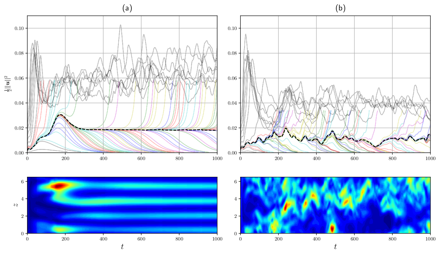
For each energy level, we generate RPs, , which we time-integrate until one of the aforementioned energy thresholds is crossed to determine the type of flow. We use RPs per energy level, except for the case for which we considered to generate more accuracy and allow for a better assessment of the control strategy. We approximate by the fraction of laminarizing RPs of energy . One may observe that due to the finite lifetime of turbulent trajectories in shear flows in small domains (Hof et al. 2006), the laminarization probability may depend on the choice of . The transient lifetimes that we observed were all, at least, an order of magnitude larger than , making our results independent on this value. We also computed the edge state kinetic energy at and using edge tracking (Skufca et al. 2006) and report the corresponding values in table 1. We demonstrate the edge tracking procedure at in figure 1(a) which yields . As can be seen from the the bottom plane in figure 1(a), the edge state for the uncontrolled case is an equilibrium structurally similar to the edge state identified in Schneider et al. 2008 in a similar domain.
To generate RPs, we first express them as a linear combination of the laminar flow field and an incompressible orthogonal component , i.e. , where , and are generated randomly, and . To ensure that has energy , we further impose . Turbulence in plane Couette flow is associated with shear concentration at the wall, yielding lower kinetic energies for the turbulent states than for the laminar flow. We thus find it intuitively useful to distinguish RPs with weakened bulk shear () from those that display stronger bulk shear (), the sets of which are hereafter called RP and RP respectively. The former can be thought of as being mostly located in phase space between the laminar (energetically higher) and the turbulent (energetically lower) flows, while the latter are located farther away from turbulence. We create such perturbations in three steps. First, we generate the random orthogonal component by drawing its spectral coefficients from the uniform distribution so that the homogeneous boundary conditions are satisfied and . Next, we draw from the uniform distribution between and and compute . To ensure that the RPs satisfy the no-slip boundary condition, we take advantage of the properties of our numerical scheme (Spalart–Moser–Rogers Runge–Kutta, see Spalart et al. 1991; leading to spatial operators solved using a Chebyshev tau algorithm, see Canuto et al. 1988) and take two (small) time-steps starting from . The resulting state is RP 11 1 For small enough time-steps, this procedure leads to negligible deviations in the energy level and in the coefficients and of the RP.. To ensure fair sampling, we use an equal number of positive and negative for each energy level.
3 Results
The results in the absence of any transition control are reported in figure 2 via the laminarization probability as a function of the RP energy at and .

We start the description from the case. For sufficiently small initial disturbance energies, the laminarization probability tends to 1, owing to the fact that the laminar flow is linearly stable. The first transitioning RP was found at the third energy level providing an upper bound for the minimal seed energy, , so that the minimal seed is located very close to the laminar fixed point. The laminarization probability decreases nearly monotonically as the RP energy increases to saturate at which we will hereafter quantify by . Most of the laminarization probability decay occurs at small amplitude, i.e., for (). For the most part, RP is responsible for the non-vanishing laminarization probability as the energy increases. The fact that does not tend to zero even for large energies is a consequence of the edge structure: it has been shown to be wrapped around the turbulent saddle such that laminarizing RP regions are locally interleaved with transitioning RP regions (Chantry & Schneider 2014), and to be fractal (Moehlis et al. 2004; Skufca et al. 2006). To understand further which RPs laminarize, we color-code them in the - plane according to their dynamics. The results for are shown in figure 3(b).

Laminarizing RPs are found for small and their number decreases as increases. Outside this clearly identifiable region, we observe very rare transitional events, evidencing the usefulness of our decomposition of the initial condition for the study of the robustness of the laminar flow. In addition, figure 3(b) shows a typical trajectory undertaken by a transitioning perturbation. This turbulent trajectory gets trapped in a small region located in the lower right corner of the figure and associated with the projection of the turbulent saddle onto the reduced subspace. This region corresponds to negative which confirms the physical reasoning behind our decomposition.
We now explore the dependence of these results on the Reynolds number. Increasing the Reynolds number from to (figures 2(c) and 3(c)) reduces the upper bound for the minimal seed energy which reflects the fact that the minimal seed energy exhibits a power-law decay as a function of (Duguet et al. 2013). Similarly, increasing reduces the edge state energy, in agreement with past studies (Wang et al. 2007). The probability associated with the distribution plateau also decreases as the Reynolds number increases ( at and at ) implying that less large-energy RPs laminarize. In general, the distribution becomes more peaked at as increases which reflects the anticipated shrinkage of the basin of attraction of the laminar flow as is increased away from criticality. We can analyse the evolution of the basin of attraction of the laminar flow with by inspecting the distribution of laminarizing and transitioning RPs in the - plane in figure 3. At , the laminarizing RPs are heavily concentrated in the region around . Decreasing slightly expands this region and, close to criticality, leads to the appearance of laminarizing RPs outside this region. Additionally, the representative transitioning trajectories shown in figure 3 indicate that the turbulent saddle expands in our projection of phase space as the Reynolds number is decreased. This reflects the fact that the variance of the turbulent kinetic energy grows as the Reynolds number is reduced towards the criticality (Faranda et al. 2014). Finally, figures 2 and 3 suggest that RP behaves similarly to RP for but that their laminarization probability tends to decrease much faster than that of RP as the Reynolds number is increased.
The probability distribution for the uncontrolled case can be approximated by the cumulative distribution function for the Gamma distribution reflected around and saturated at , i.e. , where is the lower incomplete gamma function and the values of , and are reported in table 1. The various coefficients have been determined via least-square fitting and the resulting functions are shown in figure 2 by the solid lines. One can assess control strategies by simple quantitative comparison with the distribution at a particular Reynolds number. If the action of a control strategy leads to an increase of the laminarization probability, it is successful. The difference in the shape of the laminarization probability reveals important information about the sensitivity of the laminar flow to perturbations of various amplitudes and can be used as a measure for the relative increase of the size of the basin of attraction of the laminar flow thereby quantifying control efficiency.
| , controlled | ||||
To demonstrate this, we impose in-phase spanwise wall oscillations, a strategy known to reduce the turbulent drag (Quadrio & Ricco 2004) and increase the energy of the minimal seed (Rabin et al. 2014). Under these oscillations, the modified boundary conditions read: , where , and are the amplitude, the frequency and the phase of the oscillations. The laminar flow becomes oscillatory, which modifies equation (1) into equation (2.5) of Rabin et al. 2014. We use the parameter values close to the ones considered by Rabin et al. 2014, and , and set . For these parameter values and domain size, we find that the edge state is chaotic, as shown in figure 1(b), with average kinetic energy , approximately less than for the uncontroled edge state. We generate the RPs in the same way as for the uncontrolled case, except that we also impose a random phase drawn from a uniform distribution between and .
The laminarization probability for the controlled case is shown in figure 4.

The resulting probability distribution decreases nearly monotonically to saturate around for large energy RPs. This behavior is qualitatively similar to that observed in the absence of control but fundamental quantitative differences can be reported. Firstly, the probability distribution plateaus at lower RP energy than in the uncontrolled case. This results in a larger asymptotic value of , more than double its value in the absence of wall oscillation. Secondly, a non-negligible fraction of large energy initial perturbations of RP are now found to laminarize.
that of reducing the Reynolds number in the absence of control (see figure 2(a) for Re = 400)
The effect of applying this control strategy onto transition at seems to be similar to that of reducing the Reynolds number in the absence of control (see figure 2(a) for ) despite the fact that wall oscillations effectively increase the Reynolds number by making the walls move in the spanwise direction in addition to their steady motion in the streamwise direction. An important difference can however be highlighted: this control strategy did not statistically affect the behavior of small energy perturbations from the laminar flow. To shed more light on the effect of control on the distribution of the laminarizing and transitioning RPs, we show, in figure 5, a similar representation of the initial conditions as in figure 3(b) but for the controlled case.

We recover the small region where laminarization was found in the uncontrolled case, however, we also found laminarizing RPs at larger amplitude, scattered around the region where all RPs transitioned in the absence of control. This result also bears resemblance with that at in the absence of control (see figure 3(a)). The newly controlled RPs decay via overshooting, i.e., their energy first significantly exceeds before decaying nearly monotonically. The initial phase of the RPs did not seem to play any role in determining whether or not the flow will laminarize.
The laminarization probability in the controlled case can be approximated by the fitting function , which shares the same structure as but with parameter values shown in table 1. The relative probability increase can thus be computed as averaged over the range of the considered energies. We found that this quantity is equal to so that, on average, the laminarization probability of an RP nearly doubles under the action of the aforementioned control strategy. When a single value is not satisfactory to assess the control efficiency, more detailed information can be obtained via inspecting the differences between the laminarization probabilities at each energy level.
While the fate of perturbations in the uncontrolled flow at is sensitive to the strength of the initial bulk shear measured by parameter , this is no longer the case in the presence of control via spanwise wall oscillation. Furthermore, the energy of the edge state decreases under the effect of the oscillating wall. Assuming that the edge state energy is proportional to the relative volume of the basin of attraction of the laminar fixed point, this could be interpreted as the failure of the control strategy to postpone transition but the more exhaustive analysis of phase space provided here shows that this strategy is on the contrary effective. The use of the minimal seed does not seem to provide a better basis for control assessment: the shape of the basin of attraction of the laminar flow is such that, in this study, most perturbations generated with times the energy of the minimal seed laminarized, making it difficult to extrapolate any reliable information. These observations further strengthen our approach to consider a more exhaustive method to assess control.
4 Discussion
In this paper, we have introduced a new way to analyze the robustness of the laminar flow to perturbations and to assess control strategies. We proceeded by sampling phase space in the neighbourhood of the laminar flow and evaluating the probability that the sampled initial conditions laminarize as a function of their initial energy. Our laminarisation probability bears similarities with the notion of basin stability introduced in the dynamical system context of vegetation growth (Menck et al. 2013). Our results for plane Couette flow in a small domain indicate that the laminarization probability decreases as the kinetic energy of the initial perturbation from the laminar flow is increased. It may increase back to for sufficiently large initial energy levels as a consequence of the location of the upper edge of chaos (Budanur et al. 2020). We identified that the laminarization probability decreases as the Reynods number is increased which reflects the contraction of the basin of attraction of the laminar flow. Two plausible scalar proxies for the relative volume of this basin, the edge state and the minimal seed energies, though having different asymptotic scalings with respect to , similarly reflect this expansion: their values increase as is reduced towards the criticality (Wang et al. 2007; Duguet et al. 2013).
To assess how the basin of attraction of the laminar flow changes under the action of control, the distribution of the laminarization probability obtained in the uncontrolled set-up can easily be recomputed and compared in the presence of control. We tested this methodology under control via spanwise wall oscillations at . It was shown that, under the action of similar control, the minimal seed energy increases Rabin et al. 2014 while we observed that the energy of the edge state decreases. The use of the newly introduced laminarization probability provides a much more in-depth understanding of the alteration of the robustness of the laminar flow. In particular, it revealed that the control strategy under consideration provided a major improvement in the robustness of the laminar flow, especially against large-energy perturbations. The controlled case gave similar results to the uncontrolled flow at . The laminarization probabilities differ in a subtle way: the control strategy is not efficient in laminarizing small-energy RPs but acts favourably on large-energy RPs. These observations suggest that, in contrast to the laminarization probability, scalar criteria for the robustness of the laminar flow, such as the energy of the edge state or of the minimal seed, may not be able to capture enough information to assess control strategies – the fact already noted for the edge states in the polymer drag reduction studies (Stone et al. 2002; Stone et al. 2004).
In setting up our protocol, we had to make a choice on the form of the random initial perturbation. We opted for randomizing their spectral coefficients uniformly, which might not be the ideal choice if one knows what form of perturbations are triggered in a given configuration. We stress that the current work represents a proof of concept to pave the way to customizable and more relevant protocols. There are many possibilities to constrain the initial perturbations and increase their relevance to given situations. For example, one can impose a certain shape for the spectral energy of the initial perturbations, or confine them to certain locations in the physical domain.
We believe that the methodology introduced in this paper will prove useful to control other flows (Khapko et al. 2013; Zammert & Eckhardt 2015; Watanabe et al. 2016; Chantry et al. 2017) and anticipate that, owing to the nature of transition to turbulence, it will be helpful to the study and control of a range of nonlinear systems displaying finite-amplitude instability.
Acknowledgments
This work was undertaken on ARC3, part of the High Performance Computing facilities at the University of Leeds, UK. The authors wish to thank C. Bick and R. Kerswell for fruitful discussions and the anonymous referees for their suggestions which led to a significant improvement of the paper.
Declaration of Interests
The authors report no conflict of interest.
References
- Avila et al. (2011) Avila, K., Moxey, D., de Lozar, A., Avila, M., Barkley, D. & Hof, B. 2011 The onset of turbulence in pipe flow. Science 333 (6039), 192–196.
- Baron & Quadrio (1995) Baron, A. & Quadrio, M. 1995 Turbulent drag reduction by spanwise wall oscillations. Appl. Sci. Res. 55 (4), 311–326.
- Brunton & Noack (2015) Brunton, S. L. & Noack, B. R. 2015 Closed-loop turbulence control: progress and challenges. Appl. Mech. Rev. 67 (5).
- Budanur et al. (2020) Budanur, N. B., Marensi, E., Willis, A. P. & Hof, B. 2020 Upper edge of chaos and the energetics of transition in pipe flow. Phys. Rev. Fluids 5 (2), 023903.
- Canuto et al. (1988) Canuto, C., Hussaini, M. Y., Quarteroni, A. & Zang, T. A. 1988 Spectral methods – Fundamentals in single domains. Springer-Verlag, New York .
- Chantry & Schneider (2014) Chantry, M. & Schneider, T. M. 2014 Studying edge geometry in transiently turbulent shear flows. J. Fluid Mech. 747, 506–517.
- Chantry et al. (2017) Chantry, M., Tuckerman, L. S. & Barkley, D. 2017 Universal continuous transition to turbulence in a planar shear flow. J. Fluid Mech. 824, R1.
- Dauchot & Daviaud (1995) Dauchot, O. & Daviaud, F. 1995 Finite amplitude perturbation and spots growth mechanism in plane Couette flow. Phys. Fluids 7 (2), 335–343.
- Duguet et al. (2010) Duguet, Y., Brandt, L. & Larsson, B. R. J. 2010 Towards minimal perturbations in transitional plane Couette flow. Phys. Rev. E 82 (2), 026316.
- Duguet et al. (2013) Duguet, Y., Monokrousos, A., Brandt, L. & Henningson, D. S. 2013 Minimal transition thresholds in plane Couette flow. Phys. Fluids 25 (8), 084103.
- Faranda et al. (2014) Faranda, D., Lucarini, V., Manneville, P. & Wouters, J. 2014 On using extreme values to detect global stability thresholds in multi-stable systems: The case of transitional plane Couette flow. Chaos, Solitons & Fractals 64, 26–35.
- Gibson (2014) Gibson, J. F. 2014 Channelflow: A spectral Navier–Stokes simulator in C++. Tech. Rep.. U. New Hampshire, Channelflow.org.
- Hof et al. (2010) Hof, B., De Lozar, A., Avila, M., Tu, X. & Schneider, T. M. 2010 Eliminating turbulence in spatially intermittent flows. Science 327 (5972), 1491–1494.
- Hof et al. (2006) Hof, B., Westerweel, J., Schneider, T. M. & Eckhardt, B. 2006 Finite lifetime of turbulence in shear flows. Nature 443 (7107), 59.
- Jung et al. (1992) Jung, W.-J., Mangiavacchi, N. & Akhavan, R. 1992 Suppression of turbulence in wall-bounded flows by high-frequency spanwise oscillations. Phys. Fluids A-Fluid 4 (8), 1605–1607.
- Kasagi et al. (2009) Kasagi, N., Suzuki, Y. & Fukagata, K. 2009 Microelectromechanical systems–based feedback control of turbulence for skin friction reduction. Annu. Rev. Fluid Mech. 41.
- Kawahara (2005) Kawahara, G. 2005 Laminarization of minimal plane Couette flow: going beyond the basin of attraction of turbulence. Phys. Fluids 17 (4), 041702.
- Khapko et al. (2013) Khapko, T., Kreilos, T., Schlatter, P., Duguet, Y., Eckhardt, B. & Henningson, D. S. 2013 Localized edge states in the asymptotic suction boundary layer. J. Fluid Mech. 717, R6.
- Khapko et al. (2016) Khapko, T., Kreilos, T., Schlatter, P., Duguet, Y., Eckhardt, B. & Henningson, D. S. 2016 Edge states as mediators of bypass transition in boundary-layer flows. J. Fluid Mech. 801.
- Kim & Bewley (2007) Kim, J. & Bewley, T. R. 2007 A linear systems approach to flow control. Annu. Rev. Fluid Mech. 39, 383–417.
- Marensi et al. (2019) Marensi, E., Willis, A. P. & Kerswell, R. R. 2019 Stabilisation and drag reduction of pipe flows by flattening the base profile. J. Fluid Mech. 863, 850–875.
- Mellibovsky et al. (2009) Mellibovsky, F., Meseguer, A., Schneider, T. M. & Eckhardt, B. 2009 Transition in localized pipe flow turbulence. Phys. Rev. Lett. 103 (5), 054502.
- Menck et al. (2013) Menck, P. J., Heitzig, J., Marwan, N. & Kurths, J. 2013 How basin stability complements the linear-stability paradigm. Nat. Phys. 9 (2), 89–92.
- Moehlis et al. (2004) Moehlis, J., Faisst, H. & Eckhardt, B. 2004 A low-dimensional model for turbulent shear flows. New J. Phys. 6 (1), 56.
- Olvera & Kerswell (2017) Olvera, D. & Kerswell, R. R. 2017 Optimizing energy growth as a tool for finding exact coherent structures. Phys. Rev. Fluids 2, 083902.
- Pershin et al. (2019) Pershin, A., Beaume, C. & Tobias, S. M. 2019 Dynamics of spatially localized states in transitional plane Couette flow. J. Fluid Mech. 867, 414–437.
- Pringle et al. (2012) Pringle, C. C. T., Willis, A. P. & Kerswell, R. R. 2012 Minimal seeds for shear flow turbulence: using nonlinear transient growth to touch the edge of chaos. J. Fluid Mech. 702, 415–443.
- Quadrio (2011) Quadrio, Maurizio 2011 Drag reduction in turbulent boundary layers by in-plane wall motion. Philos. Trans. R. Soc. A 369 (1940), 1428–1442.
- Quadrio & Ricco (2004) Quadrio, M. & Ricco, P. 2004 Critical assessment of turbulent drag reduction through spanwise wall oscillations. J. Fluid Mech. 521, 251–271.
- Rabin et al. (2014) Rabin, S. M. E., Caulfield, C. P. & Kerswell, R. R. 2014 Designing a more nonlinearly stable laminar flow via boundary manipulation. J. Fluid Mech. 738, R1.
- Schmiegel & Eckhardt (1997) Schmiegel, A. & Eckhardt, B. 1997 Fractal stability border in plane Couette flow. Phys. Rev. Lett. 79 (26), 5250.
- Schneider et al. (2008) Schneider, T. M., Gibson, J. F., Lagha, M., De Lillo, F. & Eckhardt, B. 2008 Laminar-turbulent boundary in plane Couette flow. Phys. Rev. E 78 (3), 037301.
- Shi et al. (2013) Shi, L., Avila, M. & Hof, B. 2013 Scale invariance at the onset of turbulence in Couette flow. Phys. Rev. Lett. 110 (20), 204502.
- Skufca et al. (2006) Skufca, J. D., Yorke, J. A. & Eckhardt, B. 2006 Edge of chaos in a parallel shear flow. Phys. Rev. Lett. 96 (17), 174101.
- Spalart et al. (1991) Spalart, P. R., Moser, R. D. & Rogers, M. M. 1991 Spectral methods for the Navier–Stokes equations with one infinite and two periodic directions. J. Comp. Phys. 96 (2), 297–324.
- Sreenivasan (1982) Sreenivasan, K. R. 1982 Laminarescent, relaminarizing and retransitional flows. Acta Mech. 44, 1–48.
- Stone et al. (2004) Stone, P. A., Roy, A., Larson, R. G., Waleffe, F. & Graham, M. D. 2004 Polymer drag reduction in exact coherent structures of plane shear flow. Phys. Fluids 16 (9), 3470–3482.
- Stone et al. (2002) Stone, P. A., Waleffe, F. & Graham, M. D. 2002 Toward a structural understanding of turbulent drag reduction: nonlinear coherent states in viscoelastic shear flows. Phys. Rev. Lett. 89 (20), 208301.
- Wang et al. (2007) Wang, J., Gibson, J. & Waleffe, F. 2007 Lower branch coherent states in shear flows: transition and control. Phys. Rev. Lett. 98 (20), 204501.
- Watanabe et al. (2016) Watanabe, T., Iima, M. & Nishiura, Y. 2016 A skeleton of collision dynamics: hierarchical network structure among even-symmetric steady pulses in binary fluid convection. SIAM J. Appl. Dyn. Sys. 15 (2), 789–806.
- Zammert & Eckhardt (2015) Zammert, S. & Eckhardt, B. 2015 Crisis bifurcations in plane Poiseuille flow. Phys. Rev. E 91, 041003(R).