跳到论文正文
W Papers独立论文阅读器 arXiv:1908.02927 论文正文 计算阅读时间 · 0%
引用这篇论文根据当前论文元数据生成,正式投稿前建议核对。


License: arXiv.org perpetual non-exclusive license
arXiv:1908.02927v1 [gr-qc] 08 Aug 2019

Analytic Keplerian-type parametrization for general spinning compact binaries with the leading order spin-orbit interactionPreprint: APS/123-QED

Gihyuk Cho 1,2, Hyung Mok Lee 2 Note: whrlsos@snu.ac.kr Affiliation: 1 Department of Physics and Astronomy, Seoul National University, Seoul 151-742, Korea
2 Korea Astronomy and Space Science Institute, 776 Daedeokdaero, Daejon, Korea
August 11, 2026
Abstract

We derive a fully analytic Keplerian-type parametrization solution to conservative motion of spinning binary in ADM gauge. This solution is able to describe three dimensional motion of binaries of arbitrary eccentricity, mass ratio and initial configuration of spin angular momentum up to the leading order of post-Newtonian(PN) approximation and a linear order in spin. Based on our results waveforms can be quickly computed with high accuracy.

I Introduction

Under Newtonian gravity which has only mass as a source, the two body problem can be analytically solved into the well-known Kepler parametrized solution. But under the Einstein gravity which has a stress energy tensor of 10 components as its source, parameters more than mass must be considered. In the classical works Mathisson 2010; Corinaldesi and Papapetrou 1951; Description 1977; Bailey and Israel 1983, multipolar expansion of stress energy tensor on a generic background metric field, has been made under the assumption that matter is highly localized in space. The results, which involve mass as a monopole contribution while spin as a dipole moment, give us understanding on how masses and spin angular momenta of point particles affect the entire dynamics. Unlike Newtonian gravity, spin angular momentum produces extra gravitational effects and thus makes orbit plane of two body and spin axes precess.
Even though dynamics of binary systems in general relativity can be solved by numerical relativity (NR) with high accuracy, it is still worth solving the equation of motion analytically. Actually, the post-Newtonian (PN) approximation which has been well established Blanchet 2014; Bernard et al. 2018, provides spin precession equation Á. Gergely et al. 1998; Gergely 1999; Blanchet et al. 2006; Faye et al. 2006 and the orbital evolution equations up to at least 4PN order Damour et al. 2014; Bernard et al. 2018. Although the PN equations can be integrated numerically with much smaller amount of computer resources than NR but analytical solution would be desirable for quick parameter estimation Veitch et al. 2015; Farr et al. 2016. Until now analytic solutions have been obtained only for some limited cases such as quasi-circular, nearly alignedKlein et al. 2013, slowly spinning Chatziioannou et al. 2013 or almost equal massKönigsdörffer and Gopakumar 2005; Tessmer 2009. General cases with arbitrary spin can be solved up to a certain PN order in terms of elliptic functions Racine 2008 and recent works present a form of the solutions partially in terms of sine-like Jacobi elliptic function with integrating out the oscillating part of orbital motion Marsat et al. 2014; Chatziioannou et al. 2017. In this paper, we present an analytic parametrized solution which involves both spin precession and orbital evolution for the binaries with arbitrary spins, masses and eccentricities of orbit. Namely, our solution parameterizes tilt angle of orbital planes and precession of spin angular momentum with respect to a fixed inertial frame, radial and angular motion of relative displacement of binaries and physical time evolution only via the eccentric anomaly, a Keplerian parameter that serves as an independent variable. Additionally because we express the entire parameterization in closed form witout any approximations, the solution is fully general.
This paper is organized as follows. In §II, dynamics which we are going to solve is presented in terms of Hamiltonian. The Hamiltonian includes Newtonian order of orbital dynamics and the leading order of spin-orbit interaction term (linear in spin). Parameters and reference frames which we choose are also presented. In §III, the ways to get the Keplerian-type parametrizations and their results are given in the following orders : Relative motion of angles between angular momenta (§III.1), the absolute precession of the orbital angular momentum in an inertial frame (§III.2), and finally, the relative position of compact binaries (§III.3). In §IV, we provide an approximant for almost equal mass case and compare it with the previous work Königsdörffer and Gopakumar 2005 as a sanity check. The final secion summarized our results.

II Dynamics with leading order of spin-orbit interaction

II.1 The Hamiltonian

In Arnowitt-Deser-Misner(ADM) type cooridnate Arnowitt et al. 2004 and with the Newton-Wigner-Pryce supplementary spin condition Newton and Wigner 1949; Pryce 1948, the (reduced) Hamiltonian HH for compact bianary systems composed of two stars with masses m1m_{1} and m2m_{2}, is as follows Wex 1995,

H=𝒑22−1r+1c2​r3​𝑳⋅𝑺eff,\displaystyle H=\frac{\bm{p}^{2}}{2}-\frac{1}{r}+\frac{1}{c^{2}r^{3}}\bm{L}\cdot\bm{S}_{\text{eff}}\,, (1)

where cc is the speed of light, 𝒓=𝑹G⁡(m1+m2)\bm{r}=\frac{\bm{R}}{G\,(m_{1}+m_{2})}, 𝒑=𝓟​(m1+m2)2m1​m2\bm{p}=\frac{\bm{\mathcal{P}}\,(m_{1}+m_{2})^{2}}{m_{1}\,m_{2}} with 𝑹\bm{R} and 𝓟\bm{\mathcal{P}} being relative position vector and conjugate momentum, respectively. The orbital angular momentum 𝑳\bm{L} and effective spin SeffS_{\text{eff}} are defined as

𝑳=𝒓×𝒑,\displaystyle\bm{L}=\bm{r}\times\bm{p}\,, (2)

and

𝑺eff=δ1​𝑺1+δ2​𝑺2.\displaystyle\bm{S}_{\text{eff}}=\delta_{1}\,\bm{S}_{1}+\delta_{2}\,\bm{S}_{2}\,. (3)

Here 𝑺1\bm{S}_{1} and 𝑺2\bm{S}_{2} are spin vectors of m1m_{1} and m2m_{2} and the waiting factors of δ1\delta_{1} and δ2\delta_{2} are,

δ1=2​m1​m2M2​(1+34​m2m1),\displaystyle\delta_{1}=2\,\frac{m_{1}\,m_{2}}{M^{2}}\left(1+\frac{3}{4}\frac{m_{2}}{m_{1}}\right)\,, (4a)
δ2=2​m1​m2M2​(1+34​m1m2).\displaystyle\delta_{2}=2\,\frac{m_{1}\,m_{2}}{M^{2}}\left(1+\frac{3}{4}\frac{m_{1}}{m_{2}}\right)\,. (4b)

For a consistent post-Newtonian approximation, we need to include the first correction of orbital dynamics (1PN) but intentionally exclude it because 1PN correction to orbital motion does not affect the spin precession at the leading order and bringing the 1PN correction into the result is expected to be straightforward Königsdörffer and Gopakumar 2005; Damour and Deruelle 1985.

II.2 The equation of motion

The equation of motion is given by Poisson bracket,

𝒓˙:=d​𝒓d​t={𝒓,H}.\displaystyle\dot{\bm{r}}:=\frac{d\bm{r}}{dt}=\{\bm{r},\,H\}\,. (5)

Likewise the corresponding angular momentum and spin precession equations are given as

d​𝑳d​t\displaystyle\frac{d\bm{L}}{dt} ={𝑳,H}=1c2​r3​𝑺eff×𝑳,\displaystyle=\{\bm{L},\,H\}=\frac{1}{c^{2}\,r^{3}}\,\bm{S}_{\text{eff}}\times\bm{L}\,, (6a)
d​𝑺1d​t\displaystyle\frac{d\bm{S}_{1}}{dt} ={𝑺1,H}=δ1c2​r3​𝑳×𝑺1,\displaystyle=\{\bm{S}_{1},\,H\}=\frac{\delta_{1}}{c^{2}\,r^{3}}\,\bm{L}\times\bm{S}_{1}\,, (6b)
d​𝑺2d​t\displaystyle\frac{d\bm{S}_{2}}{dt} ={𝑺2,H}=δ2c2​r3​𝑳×𝑺2,\displaystyle=\{\bm{S}_{2},\,H\}=\frac{\delta_{2}}{c^{2}\,r^{3}}\,\bm{L}\times\bm{S}_{2}\,, (6c)

by invoking the fact that angular momentum is a generator of rotations i.e.

{Si,Sj}=ϵi​j​k​Sk.\displaystyle\{S_{i},S_{j}\}=\epsilon_{ijk}\,S_{k}\,. (7)

From the evolution of angular momentum and spins, we can find several conserved quantities that can be exploited in deriving the dynamical solutions. First, the magnitudes of the angular momenta are conserved because

d⁡(𝑳⋅𝑳)d​t=2c2​r3​𝑳⋅(𝑺eff×𝑳)=0,\displaystyle\frac{d(\bm{L}\cdot\bm{L})}{dt}=\frac{2}{c^{2}\,r^{3}}\,\bm{L}\cdot(\bm{S}_{\text{eff}}\times\bm{L})=0\,, (8a)
d⁡(𝑺1⋅𝑺1)d​t=2​δ1c2​r3​𝑺1⋅(𝑳×𝑺1)=0,\displaystyle\frac{d(\bm{S}_{1}\cdot\bm{S}_{1})}{dt}=\frac{2\,\delta_{1}}{c^{2}\,r^{3}}\,\bm{S}_{1}\cdot(\bm{L}\times\bm{S}_{1})=0\,, (8b)
d⁡(𝑺2⋅𝑺2)d​t=2​δ2c2​r3​𝑺2⋅(𝑳×𝑺2)=0.\displaystyle\frac{d(\bm{S}_{2}\cdot\bm{S}_{2})}{dt}=\frac{2\,\delta_{2}}{c^{2}\,r^{3}}\,\bm{S}_{2}\cdot(\bm{L}\times\bm{S}_{2})=0\,. (8c)

Also in the absence of the angular momentum loss from the binary system, the total angular momentum 𝑱=𝑳+𝑺1+𝑺2\bm{J}=\bm{L}+\bm{S}_{1}+\bm{S}_{2} is conserved. Without loss of generality we can define the z-axis of the inertial frame to be aligned with 𝑱\bm{J} while the the orthogonal axes xx and yy can be chosen arbitrarily on the plane perpendicular to zz-axis as shown in Fig. 1.

Refer to caption
Figure 1: Two bases are displayed : The inertial frame (𝒆x,𝒆y,𝒆z)(\bm{e}_{x},\,\bm{e}_{y},\,\bm{e}_{z}) and the non-inertial frame (𝒊,𝒋,𝒌)(\bm{i},\,\bm{j},\,\bm{k}). The total angular momentum 𝑱\bm{J} is parallel to 𝒆z\bm{e}_{z}, and the orbital angular momentum 𝑳\bm{L} to 𝒌\bm{k}. The non-inertial frame is constructed by rotating the inertial frame around zz-axis by ξ1\xi_{1} and then around xx-axis by ξ2\xi_{2}, so that ξ1\xi_{1} and ξ2\xi_{2} determine the orientation of 𝑳\bm{L}.

At the same time, we define an orthonormal non inertial frame (𝒊,𝒋,𝒌)(\bm{i},\bm{j},\bm{k}),

(𝒊𝒋𝒌)=Λ​(𝒆x𝒆y𝒆z)\displaystyle\left(\begin{array}[]{ccc}\bm{i}\\ \bm{j}\\ \bm{k}\\ \end{array}\right)=\Lambda\,\left(\begin{array}[]{ccc}\bm{e}_{x}\\ \bm{e}_{y}\\ \bm{e}_{z}\\ \end{array}\right)

where Λ\Lambda is the Euler matrix as shown below

Λ=(cos⁡ξ1sin⁡ξ10−sinξ1cosξ2cosξ1cosξ2sin⁡ξ2sinξ1sinξ2−cosξ1sinξ2cos⁡ξ2).\displaystyle\Lambda=\left(\begin{array}[]{ccc}\cos\xi_{1}&\sin\xi_{1}&0\\ -\sin\xi_{1}\,\cos\xi_{2}&\cos\xi_{1}\,\cos\xi_{2}&\sin\xi_{2}\\ \sin\xi_{1}\sin\xi_{2}&-\cos\xi_{1}\sin\xi_{2}&\cos\xi_{2}\\ \end{array}\right)\,.

The geometric meaning of the Euler matrix is presented in Fig. 1.
Next, we define the angles γ\gamma, κ1\kappa_{1} and κ2\kappa_{2} in the range of [0,π][0,\,\pi] such that

cos⁡γ:=𝑺1⋅𝑺2S1​S2,\displaystyle\cos\gamma:=\frac{\bm{S}_{1}\cdot\bm{S}_{2}}{S_{1}\,\,S_{2}}\,, (18a)
cos⁡κ1:=𝑳⋅𝑺1L​S1,\displaystyle\cos\kappa_{1}:=\frac{\bm{L}\cdot\bm{S}_{1}}{L\,\,S_{1}}\,, (18b)
cos⁡κ2:=𝑳⋅𝑺2L​S2,\displaystyle\cos\kappa_{2}:=\frac{\bm{L}\cdot\bm{S}_{2}}{L\,\,S_{2}}\,, (18c)

as illustrated in Fig. 2.

Refer to caption
Figure 2: The geometry of spin and angular momentum vectors, and the inertial frame.

The rates of changes of these angles are given via Eq.(6) i.e.

d​cos⁡γd​t\displaystyle\frac{d\cos\gamma}{dt} =δ1−δ2c2​r3​S1​S2​𝑳⋅(𝑺1×𝑺2),\displaystyle=\,\frac{\delta_{1}-\delta_{2}}{c^{2}\,r^{3}\,S_{1}\,S_{2}}\bm{L}\cdot(\bm{S}_{1}\times\bm{S}_{2})\,, (19a)
dcosκ1d​t\displaystyle\frac{d\cos\kappa_{1}}{dt} =δ2c2​r3​S1​L​𝑳⋅(𝑺1×𝑺2),\displaystyle=\,\frac{\delta_{2}}{c^{2}\,r^{3}\,S_{1}\,L}\bm{L}\cdot(\bm{S}_{1}\times\bm{S}_{2})\,, (19b)
dcosκ2d​t\displaystyle\frac{d\cos\kappa_{2}}{dt} =−δ1c2​r3​S2​L𝑳⋅(𝑺1×𝑺2).\displaystyle=\,-\frac{\delta_{1}}{c^{2}\,r^{3}\,S_{2}\,L}\bm{L}\cdot(\bm{S}_{1}\times\bm{S}_{2})\,. (19c)

By observing their common factor 𝑳⋅(𝑺1×𝑺2)\bm{L}\cdot(\bm{S}_{1}\times\bm{S}_{2}), we can define new conserved quantities σ1\sigma_{1}, σ2\sigma_{2} as follows

σ1\displaystyle\sigma_{1}\, :=cosγ−LS2δ1−δ2δ2cosκ1,\displaystyle:=\cos\gamma-\frac{L}{S_{2}}\frac{\delta_{1}-\delta_{2}}{\delta_{2}}\cos\kappa_{1}\,, (20a)
σ2\displaystyle\sigma_{2}\, :=cosκ2+δ1δ2S1S2cosκ1.\displaystyle:=\cos\kappa_{2}+\frac{\delta_{1}}{\delta_{2}}\frac{S_{1}}{S_{2}}\cos\kappa_{1}\,. (20b)

Note that if δ1−δ2=0\delta_{1}-\delta_{2}=0, or equal mass case, then σ1=cos⁡γ\sigma_{1}=\cos\gamma implying that the angle γ\gamma between 𝑺1\bm{S}_{1} and 𝑺2\bm{S}_{2} is conserved.
Through straightforward vector algebra, one can show that 𝑳⋅(𝑺1×𝑺2)=LS1S2sinκ1sinκ2sinΔψ\bm{L}\cdot(\bm{S}_{1}\times\bm{S}_{2})=L\,S_{1}\,S_{2}\,\sin\kappa_{1}\sin\kappa_{2}\sin\Delta\psi, where Δ​ψ\Delta\psi is an angle between the projection of 𝑺1\bm{S}_{1} and 𝑺2\bm{S}_{2} onto x-y plane of the non-inertial frame where 𝑳\bm{L} is along with zz-axis (See Fig. 2). It has the following relation with the others,

cos⁡Δ​ψ=cosγ−cosκ1cosκ2sinκ1sinκ2.\displaystyle\cos\Delta\psi=\frac{\cos\gamma-\cos\kappa_{1}\,\cos\kappa_{2}}{\sin\kappa_{1}\,\sin\kappa_{2}}\,. (21)

When either sin⁡κ1=0\sin\kappa_{1}=0 or sin⁡κ2=0\sin\kappa_{2}=0, Δ​ψ\Delta\psi is not defined in the geometric sense. But physically we can extend the definition of Δ​ψ\Delta\psi properly. For example let us assume that κ1=0\kappa_{1}=0 and sin⁡κ2≠0\sin\kappa_{2}\neq 0 at the initial time t0t_{0}. Then, during an infinitesimal time interval d​tdt, d​𝑺1=0d\bm{S}_{1}=0 because |d​𝑺1d​t|∼|𝑳×𝑺1|∼sin⁡κ1=0|\frac{d\bm{S}_{1}}{dt}|\sim|\bm{L}\times\bm{S}_{1}|\sim\sin\kappa_{1}=0. On the other hand, d𝑳=𝑳(t0+dt)−𝑳(t0)=−d​t​δ2c2​r3𝑳×𝑺2d\bm{L}=\bm{L}(t_{0}+dt)-\bm{L}(t_{0})=-\frac{dt\,\delta_{2}}{c^{2}\,r^{3}}\bm{L}\times\bm{S}_{2}. Therefore the square of the d​𝑳d\bm{L} is given as

|𝑳⁡(t0+d​t)−𝑳⁡(t0)|2=d​t 2​(LS2δ2sinκ2c2​r3)2.\displaystyle\big|\bm{L}(t_{0}+dt)-\bm{L}(t_{0})\big|^{2}=dt^{\,2}\,\left(\frac{L\,S_{2}\,\delta_{2}\,\sin\kappa_{2}}{c^{2}\,r^{3}}\right)^{2}\,. (22)

Because 𝑳⁡(t0)\bm{L}(t_{0}) and 𝑺1​(t0)\bm{S}_{1}(t_{0}) are aligned and 𝑺1​(t0+d​t)=𝑺1​(t0)\bm{S}_{1}(t_{0}+dt)=\bm{S}_{1}(t_{0}), the infinitesimal change of κ1\kappa_{1} is the angle between 𝑳⁡(t0+d​t)\bm{L}(t_{0}+dt) and 𝑳⁡(t0)\bm{L}(t_{0}) . Thus the right hand side of Eq.(22) is

2​L2​(1−cos⁡d​κ1)=L2​d​κ1 2+O⁡(d​κ1 3).\displaystyle 2\,L^{2}\,(1-\cos d\kappa_{1})=L^{2}\,d\kappa_{1}^{\,2}\,+O(d\kappa_{1}^{\,3}). (23)

Since κ1\kappa_{1} can only increase during d​tdt, we get d​κ1d​t=δ2S2sinκ2c2​r3\frac{d\kappa_{1}}{dt}=\frac{\delta_{2}\,S_{2}\,\sin\kappa_{2}}{c^{2}\,r^{3}}. Thus by setting sin⁡Δ​ψ=−1\sin\Delta\psi=-1, replacing the vectorial expression 𝑳⋅(𝑺1×𝑺2)\bm{L}\cdot(\bm{S}_{1}\times\bm{S}_{2}) in Eqs.(19) to the algebraic expression LS1S2sinκ1sinκ2sinΔψL\,S_{1}\,S_{2}\,\sin\kappa_{1}\sin\kappa_{2}\sin\Delta\psi becomes valid even in the case of κ1=0\kappa_{1}=0. Likewise we arrive at same extension sin⁡Δ​ψ=−1\sin\Delta\psi=-1 when κ2=π\kappa_{2}=\pi (with sin⁡κ1≠0\sin\kappa_{1}\neq 0), while sin⁡Δ​ψ=1\sin\Delta\psi=1 in the case of κ1=π\kappa_{1}=\pi (sin⁡κ2≠0\sin\kappa_{2}\neq 0) and κ2=0\kappa_{2}=0 (sin⁡κ1≠0\sin\kappa_{1}\neq 0). Mathematically, this kind of extension is nothing but taking the limit of sin⁡κ1,2→0\sin\kappa_{1,2}\rightarrow 0 along the physically preferred paths. If sin⁡κ1=0\sin\kappa_{1}=0 and sin⁡κ2=0\sin\kappa_{2}=0 are both satisfied at some point, since every angle becomes constant, we do not need to define Δ​ψ\Delta\psi.

We have three time dependent variables κ1​(t)\kappa_{1}(t), κ2​(t)\kappa_{2}(t) and γ⁡(t)\gamma(t) to solve and two conserved quantities, σ1\sigma_{1} and σ2\sigma_{2}. So, if we determine a numerical value of any one angle (say κ1\kappa_{1}), the others are determined automatically by the initially fixed values of σ1\sigma_{1} and σ2\sigma_{2}. This fact allows the relations of Eqs.(19), where κ1\kappa_{1}, κ2\kappa_{2} and γ\gamma are non-linearly entangled, to be expressed in a single variable equation, for example κ1\kappa_{1}. This specific choice of κ1\kappa_{1} is followed from the fact that γ\gamma is not a good parameter. As mentioned earlier, γ\gamma fails to parametrize the dynamics when mass ratio becomes close to 1. Choosing γ\gamma as a paramter was used in Kesden et al. 2015, and we can see that there are divergences as q→1q\rightarrow 1 in the equations (7a) and (7b) in Kesden et al. 2015.

III The Keplerian-type parametrization

III.1 The Keplerian-type parametrization of the Angles

In this section, we solve the Eq.(19)s. We reduce the common factor 𝑳⋅(𝑺1×𝑺2)\bm{L}\cdot(\bm{S}_{1}\times\bm{S}_{2}), using σ1\sigma_{1} and σ2\sigma_{2}, into single variable (cos⁡κ1\cos\kappa_{1}) dependent expression,

𝑳⋅(𝑺1×𝑺2)L​S1​S2=sinκ1sinκ2sinΔψ,\displaystyle\frac{\bm{L}\cdot(\bm{S}_{1}\times\bm{S}_{2})}{L\,S_{1}\,S_{2}}=\sin\kappa_{1}\sin\kappa_{2}\sin\Delta\psi\,, (24)
=\displaystyle= ±1−cos2κ1−cos2κ2−cos2γ+2cosγcosκ1cosκ2\displaystyle\,\pm\sqrt{1-\cos^{2}\kappa_{1}-\cos^{2}\kappa_{2}-\cos^{2}\gamma+2\cos\gamma\cos\kappa_{1}\cos\kappa_{2}}\,
=\displaystyle= ±δ2​S2{−2δ1LS1(δ1−δ2)cos3κ1−[L2(δ1−δ2)2+2δ2Lσ2S2(δ2−δ1)+δ12S12+2δ1δ2σ1S1S2+δ22S22]cos2κ1\displaystyle\,\frac{\pm}{\delta_{2}\,S_{2}}\bigg\{-2\,\delta_{1}\,L\,S_{1}(\delta_{1}-\delta_{2})\cos^{3}\kappa_{1}-\big[L^{2}\,(\delta_{1}-\delta_{2})^{2}+2\,\delta_{2}\,L\,\sigma_{2}\,S_{2}\,(\delta_{2}-\delta_{1})+\delta_{1}^{2}\,S_{1}^{2}+2\,\delta_{1}\,\delta_{2}\,\sigma_{1}\,S_{1}\,S_{2}+\delta_{2}^{2}\,S_{2}^{2}\big]\,\cos^{2}\kappa_{1}
+2δ2S2[Lσ1(δ2−δ1)+σ2(δ1S1+δ2σ1S2)]cosκ1−δ22S22(σ12+σ22−1)}1/2.\displaystyle+2\,\delta_{2}\,S_{2}\,\big[L\,\sigma_{1}\,(\delta_{2}-\delta_{1})+\sigma_{2}\,(\delta_{1}S_{1}+\delta_{2}\sigma_{1}S_{2})\big]\,\cos\kappa_{1}-\delta_{2}^{2}\,S_{2}^{2}\,(\sigma_{1}^{2}+\sigma_{2}^{2}-1)\bigg\}^{1/2}\,.

The sign of 𝑳⋅(𝑺1×𝑺2)\bm{L}\cdot(\bm{S}_{1}\times\bm{S}_{2}) is determined by the sign of sin⁡Δ​ψ\sin\Delta\psi. For simplicity, let us denote cos⁡κ1=x\cos\kappa_{1}=x and factorize the expression inside the square root in terms of its 3rd polynomial roots of x=(x1,x2,x3)x=(x_{1},x_{2},x_{3}) and introduce a coefficient A:=2​L​S1​δ1​(δ2−δ1)A:=2\,L\,S_{1}\,\delta_{1}\,(\delta_{2}-\delta_{1}) to simplify the above equation as

𝑳⋅(𝑺1×𝑺2)L​S1​S2=±δ2​S2​A⁡(x−x1)​(x−x2)​(x−x3).\displaystyle\frac{\bm{L}\cdot(\bm{S}_{1}\times\bm{S}_{2})}{L\,S_{1}\,S_{2}}=\,\frac{\pm}{\delta_{2}\,S_{2}}\sqrt{A\,(x-x_{1})(x-x_{2})(x-x_{3})}\,. (25)

Before proceeding integrations, one needs to clarify the existence of the real roots of xx. Here is a brief proof: Let us assume that there is no instance such that κ1​(t)\kappa_{1}(t), κ2​(t)\kappa_{2}(t) and γ⁡(t)\gamma(t) satisfy 𝑳⋅(𝑺1×𝑺2)=0\bm{L}\cdot(\bm{S}_{1}\times\bm{S}_{2})=0 during evolutions. This assumption says that if 𝑳⋅(𝑺1×𝑺2)>0\bm{L}\cdot(\bm{S}_{1}\times\bm{S}_{2})>0 initially this inequalitiy always holds by virtue of continuity. Also the followings hold forever, dcosκ1d​t>0\frac{d\cos\kappa_{1}}{dt}>0, d​cos⁡γd​t>0\frac{d\cos\gamma}{dt}>0 (if δ1>δ2\delta_{1}>\delta_{2}) and dcosκ2d​t<0\frac{d\cos\kappa_{2}}{dt}<0. Then we are able to find a real value TT such that cos⁡κ1>0\cos\kappa_{1}>0, cos⁡γ>0\cos\gamma>0 and cos⁡κ2<0\cos\kappa_{2}<0 at times t>Tt>T unless dcosκ1d​t→0+\frac{d\cos\kappa_{1}}{dt}\rightarrow 0+, d​cos⁡γd​t→0+\frac{d\cos\gamma}{dt}\rightarrow 0+ and dcosκ2d​t→0−\frac{d\cos\kappa_{2}}{dt}\rightarrow 0- fast enough as t→∞t\rightarrow\infty. But we exclude this dissipative possibility because governing dynamics is symmetric under the reflection of t→−tt\rightarrow-t.
Meanwhile the time derivative of 𝑳⋅(𝑺1×𝑺2)\bm{L}\cdot(\bm{S}_{1}\times\bm{S}_{2}) is

d​𝑳⋅(𝑺1×𝑺2)d​t\displaystyle\frac{d\bm{L}\cdot(\bm{S}_{1}\times\bm{S}_{2})}{dt} (26)
=\displaystyle= −2cosκ1+2cosγcosκ2𝑳⋅(𝑺1×𝑺2)​dcosκ1d​t\displaystyle\frac{-2\cos\kappa_{1}+2\cos\gamma\,\cos\kappa_{2}}{\bm{L}\cdot(\bm{S}_{1}\times\bm{S}_{2})}\frac{d\cos\kappa_{1}}{dt}
+\displaystyle+ −2cosκ2+2cosγcosκ1𝑳⋅(𝑺1×𝑺2)​dcosκ2d​t\displaystyle\frac{-2\cos\kappa_{2}+2\cos\gamma\,\cos\kappa_{1}}{\bm{L}\cdot(\bm{S}_{1}\times\bm{S}_{2})}\frac{d\cos\kappa_{2}}{dt}
+\displaystyle+ −2cosγ+2cosκ1cosκ2𝑳⋅(𝑺1×𝑺2)​d​cos⁡γd​t.\displaystyle\frac{-2\cos\gamma+2\cos\kappa_{1}\,\cos\kappa_{2}}{\bm{L}\cdot(\bm{S}_{1}\times\bm{S}_{2})}\frac{d\cos\gamma}{dt}\,.

It is obvious that d​𝑳⋅(𝑺1×𝑺2)d​t<0\frac{d\bm{L}\cdot(\bm{S}_{1}\times\bm{S}_{2})}{dt}<0 when t>Tt>T. Similarly we can estimate its second time derivative and we can decompose it into two components i.e. d2​𝑳⋅(𝑺1×𝑺2)d​t2=A^​(t)+B^​(t)​r˙\frac{d^{2}\bm{L}\cdot(\bm{S}_{1}\times\bm{S}_{2})}{dt^{2}}=\hat{A}(t)+\hat{B}(t)\,\dot{r} where A^​(t)<0\hat{A}(t)<0, B^​(t)>0\hat{B}(t)>0 but r˙\dot{r} oscillates sinusoidally between positive and negative values with zero averaged value i.e. 12​π​∫02​πd​u​r˙=0\frac{1}{2\pi}\int_{0}^{2\pi}du\,\dot{r}=0. Thus in much longer time scale than one orbital period, the absolute value of d​𝑳⋅(𝑺1×𝑺2)d​t\frac{d\bm{L}\cdot(\bm{S}_{1}\times\bm{S}_{2})}{dt} increases, i.e. decreasing of 𝑳⋅(𝑺1×𝑺2)\bm{L}\cdot(\bm{S}_{1}\times\bm{S}_{2}) accelerates. This suggests that at some point 𝑳⋅(𝑺1×𝑺2)\bm{L}\cdot(\bm{S}_{1}\times\bm{S}_{2}) will pass zero, or 𝑳⋅(𝑺1×𝑺2)>0\bm{L}\cdot(\bm{S}_{1}\times\bm{S}_{2})>0 cannot hold forever. This is contradictory to the assumption. Likewise another assumption that 𝑳⋅(𝑺1×𝑺2)<0\bm{L}\cdot(\bm{S}_{1}\times\bm{S}_{2})<0 also encounters the same contradiction. Finally we come to the conclusion that whatever the initial condition is, binary systems eventually meet the configuration which corresponds to 𝑳⋅(𝑺1×𝑺2)=0\bm{L}\cdot(\bm{S}_{1}\times\bm{S}_{2})=0. Actually this happens twice, once when 𝑳⋅(𝑺1×𝑺2)\bm{L}\cdot(\bm{S}_{1}\times\bm{S}_{2}) is increasing or once when it is decreasing. Let us match cosine value of these two κ1\kappa_{1} values to x2x_{2} and x3x_{3}. Then it is obvious that they are real and the absolute values are less than or equal to 11. Additionally, from the fact that cubic polynomicals of which all coefficients are real, cannot have two real roots and a single complex root, we can conclude that x1x_{1} is also real. Note that our assumption does not include the equal mass case, i.e., δ1=δ2\delta_{1}=\delta_{2} in the above proof. Since there is no reason for any discontinuity toward the equal mass case, we can extend the validity of our formalism to δ1=δ2\delta_{1}=\delta_{2} although we need a special caution in applying the formalism presented below when two masses become very close. The case of nearly equal mass is treated separately in §IV.

Without loss of generality, we assume that A>0A>0 and x2≤cos⁡κ1≤x3x_{2}\leq\cos\kappa_{1}\leq x_{3}, because it must be non negative within the square root as illustrated in Fig. 3.
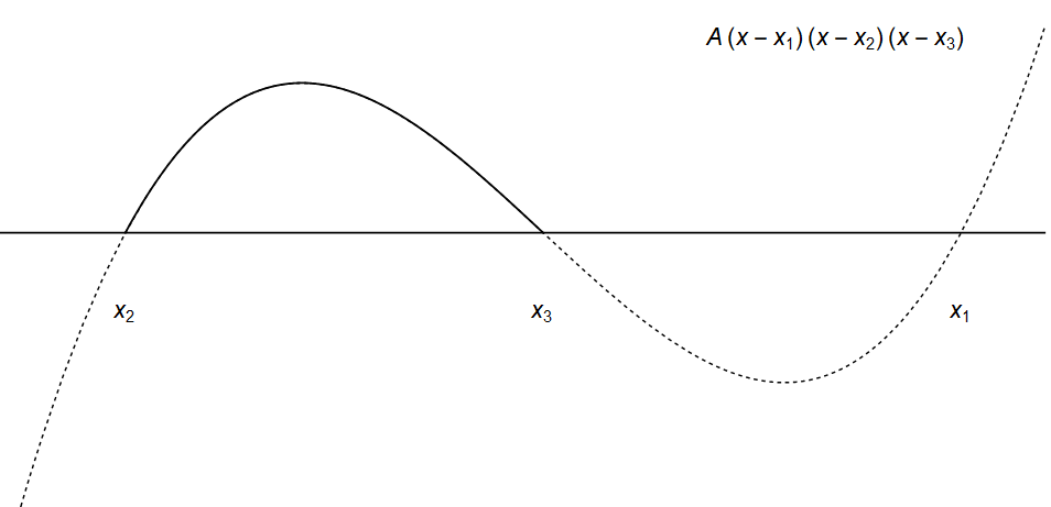
Refer to caption
Figure 3: The shape of the function inside the square-root of Eq.(24).

Eq.(19b) becomes,

d​xd​t\displaystyle\frac{dx}{dt} =±c2​r3​A⁡(x−x1)​(x−x2)​(x−x3),\displaystyle=\frac{\pm}{c^{2}\,r^{3}}\sqrt{A(x-x_{1})(x-x_{2})(x-x_{3})}\,, (27)

or,

dcosκ1A⁡(cos⁡κ1−x1)​(cos⁡κ1−x2)​(cos⁡κ1−x3)=±d​tc2​r3.\displaystyle\frac{\,d\cos\kappa_{1}}{\sqrt{A(\cos\kappa_{1}-x_{1})(\cos\kappa_{1}-x_{2})(\cos\kappa_{1}-x_{3})}}=\frac{\pm\,dt}{c^{2}\,r^{3}}. (28)

It is enough that rr is given in the Newtonian order, because we restrict the spin orbit interaction only up to the leading order. In Newtonian order we can use the well known expressions of r=a⁡(1−e​cos⁡u)r=a\,(1-e\,\cos u) and n⁡(t−t0)=u−e​sin⁡un\,(t-t_{0})=u-e\,\sin u, where uu is the eccentric anomaly, nn is the mean angular speed and tt is physical time with an initial value t0t_{0} when u=0u=0, aa is the semi-major axis of the ellipse, and ee is the eccentricity. Thus the right hand side of Eq.(28) can be integrated to

(r.h.s)=\displaystyle(r.h.s)= ∫d​u​d​td​u​±1c2​r3\displaystyle\int du\frac{dt}{du}\frac{\pm 1}{c^{2}\,r^{3}}
=\displaystyle= α±ν+e​sin⁡νc2​n​a3​(1−e2)3/2,\displaystyle\alpha\pm\frac{\nu+e\sin\nu}{c^{2}\,n\,a^{3}\,(1-e^{2})^{3/2}}\,,
=\displaystyle= α±ν+e​sin⁡νc2​L3+O⁡(1c3),\displaystyle\alpha\pm\frac{\nu+e\sin\nu}{c^{2}\,L^{3}}\,+O(\frac{1}{c^{3}}), (29)

where we use the Newtonian expression of the magnitude of the orbital angular momentum L=n13​a​(1−e2)12+O⁡(1c)L=n^{\frac{1}{3}}\,a\,(1-e^{2})^{\frac{1}{2}}+O(\frac{1}{c}) with ν=2​arctan⁡(1+e1−e​tan⁡u2)\nu=2\,\arctan(\sqrt{\frac{1+e}{1-e}}\,\tan\frac{u}{2}) and α\alpha refers to proper initial value which will be defined later. Note that the given expression of Eq.(III.1) is somewhat deceiving. Because the ±\pm sign in front of ν\nu dependent term changes as cos⁡κ1\cos\kappa_{1} passes its maximum x3x_{3} or minimum x2x_{2}. For example, if cos⁡κ1\cos\kappa_{1} arrives at x3x_{3} when ν=ν3\nu=\nu_{3}, then when ν>ν3\nu>\nu_{3} it would be better if right hand side of Eq.(III.1) is written as

α+2​ν3+esinν3c2​L3−ν+e​sin⁡νc2​L3,\displaystyle\alpha+2\,\frac{\nu_{3}+e\sin\nu_{3}}{c^{2}\,L^{3}}-\frac{\nu+e\sin\nu}{c^{2}\,L^{3}}\,, (30)

hence it has a periodic structure behind and more complicated feature than presented in Eq.(III.1). But as we can see later, the presented expression of Eq.(III.1) will be justified.
Now let us solve the left hand side of Eq.(28) keeping in mind that x2≤x≤x3<x1x_{2}\leq x\leq x_{3}<x_{1},

(l.h.s)=d​xA⁡(x−x1)​(x−x2)​(x−x3)\displaystyle(l.h.s)=\frac{dx}{\sqrt{A(x-x_{1})(x-x_{2})(x-x_{3})}} (31)
=\displaystyle= d​xA⁡(x1−x2)​x1−xx1−x2​x−x2​x3−x2​x3−xx3−x2\displaystyle\frac{dx}{\sqrt{A(x_{1}-x_{2})}\sqrt{\frac{x_{1}-x}{x_{1}-x_{2}}}\sqrt{x-x_{2}}\sqrt{x_{3}-x_{2}}\sqrt{\frac{x_{3}-x}{x_{3}-x_{2}}}}
=\displaystyle= 1x3−x2​1x−x2​d​xA⁡(x1−x2)​1−x3−x2x1−x2​x−x2x3−x2​1−x−x2x3−x2.\displaystyle\frac{\frac{1}{\sqrt{x_{3}-x_{2}}}\frac{1}{\sqrt{x-x_{2}}}dx}{\sqrt{A(x_{1}-x_{2})}\sqrt{1-\frac{x_{3}-x_{2}}{x_{1}-x_{2}}\frac{x-x_{2}}{x_{3}-x_{2}}}\sqrt{1-\frac{x-x_{2}}{x_{3}-x_{2}}}}.

Since 0≤x−x2x3−x2≤10\leq\frac{x-x_{2}}{x_{3}-x_{2}}\leq 1, we can introduce a new variable yy defined through

sin2⁡y=x−x2x3−x2\displaystyle\sin^{2}y=\frac{x-x_{2}}{x_{3}-x_{2}}\, (32)

which is restricted to 0≤y≤π20\leq y\leq\frac{\pi}{2}. Then the last line of the Eq.(31) becomes

1x3−x2​1x−x2​d​xA⁡(x1−x2)​1−x3−x2x1−x2​sin2⁡y​cos⁡y\displaystyle\frac{\frac{1}{\sqrt{x_{3}-x_{2}}}\frac{1}{\sqrt{x-x_{2}}}dx}{\sqrt{A(x_{1}-x_{2})}\sqrt{1-\frac{x_{3}-x_{2}}{x_{1}-x_{2}}\sin^{2}y}\,\cos y} (33)
=\displaystyle= 2​d​yA⁡(x1−x2)​1−x3−x2x1−x2​sin2⁡y.\displaystyle\frac{2\,dy}{\sqrt{A(x_{1}-x_{2})}\sqrt{1-\frac{x_{3}-x_{2}}{x_{1}-x_{2}}\sin^{2}y}}\,.

Identifying this integral as the Elliptic Integral of the first kind FF,

F⁡(ϕ,k):=∫ϕd​θ1−k2​sin2⁡θ,\displaystyle F(\phi,\,k):=\int^{\phi}\frac{d\theta}{\sqrt{1-k^{2}\,\sin^{2}\theta}}\,, (34)

the Eq.(33) can be written in the following compact form

2A⁡(x1−x2)​F​(arcsin⁡cos⁡κ1−x2x3−x2,x3−x2x1−x2).\displaystyle\frac{2}{\sqrt{A(x_{1}-x_{2})}}\,F\left(\arcsin\sqrt{\frac{\cos\kappa_{1}-x_{2}}{x_{3}-x_{2}}},\sqrt{\frac{x_{3}-x_{2}}{x_{1}-x_{2}}}\right)\,. (35)

There could be other possible forms instead of Eq.(35) but, under the assumption of x2≤cos⁡κ1≤x3x_{2}\leq\cos\kappa_{1}\leq x_{3}, the above form is well defined.
Finally by integrating both sides of Eq.(28), Keplerian parametrization of cos⁡κ1\cos\kappa_{1} can be obtained as,

cos⁡κ1\displaystyle\cos\kappa_{1}\, =x2+(x3−x2)​sn2​(Υ,β)\displaystyle=\,x_{2}+(x_{3}-x_{2})\,\text{sn}^{2}(\Upsilon\,,\,\beta)\, (36)
=x2​cn2​(Υ,β)+x3​dn2​(Υ,β),\displaystyle=x_{2}\,\text{cn}^{2}(\Upsilon\,,\,\beta)+x_{3}\,\text{dn}^{2}(\Upsilon\,,\,\beta)\,,

where Υ=A⁡(x1−x2)2​(α+ν+e​sin⁡νc2​L3)\Upsilon=\frac{\sqrt{A(x_{1}-x_{2})}}{2}(\alpha+\frac{\nu+e\sin\nu}{c^{2}\,L^{3}}), β=x3−x2x1−x2\beta=\sqrt{\frac{x_{3}-x_{2}}{x_{1}-x_{2}}} and sn,cn\text{sn},\text{cn} and dn are the sine, cosine and tangent like Jacobi elliptic functions Whittaker and Watson 2009.
It is worth pointing out that ±\pm sign which was supposed to be inside the definition of Υ\Upsilon according to Eq.(III.1), is removed. Because of symmetric property, sn2​(X,b)=sn2​(−X,b)\text{sn}^{2}(X,b)=\text{sn}^{2}(-X,b), we have a freedom to choose definition of Υ\Upsilon among four cases of ±A⁡(x1−x2)2​(α±ν+e​sin⁡νc2​L3)\pm\frac{\sqrt{A(x_{1}-x_{2})}}{2}(\alpha\pm\frac{\nu+e\sin\nu}{c^{2}\,L^{3}}). Firstly, we have chosen A⁡(x1−x2)2​(±α+ν+e​sin⁡νc2​L3)\frac{\sqrt{A(x_{1}-x_{2})}}{2}(\pm\alpha+\frac{\nu+e\sin\nu}{c^{2}\,L^{3}}) so that the sign of ν\nu dependent term is positive. And we make ±\pm sign in front of α\alpha be absorbed into the definition of α\alpha. That is,

α=±2A⁡(x1−x2)​F​(arcsin⁡cos⁡κ1​(0)−x2x3−x2,β),\displaystyle\alpha=\pm\frac{2}{\sqrt{A(x_{1}-x_{2})}}\,F\left(\arcsin\sqrt{\frac{\cos\kappa_{1(0)}-x_{2}}{x_{3}-x_{2}}},\,\beta\right)\,, (37)

where cos⁡κ1​(0)\cos\kappa_{1(0)} is an initial value of cos⁡κ1\cos\kappa_{1} when t=t0t=t_{0}, or u=0u=0. The ±\pm sign is determined as : ++ for the case that dcosκ1d​t>0\frac{d\cos\kappa_{1}}{dt}>0 initially while −- for dcosκ1d​t<0\frac{d\cos\kappa_{1}}{dt}<0 initially. Lastly, as we have seen, the expression of Eq.(III.1) could not capture its oscillating feature. But we do not need to be concerned of it since the final form of our solution Eq.(36) trivially captures the feature. Taking Eq.(30) as an example again, the reflection symmetry of sn, sn​(X+b,d)=sn​(X−b,d)\text{sn}(X+b,d)=\text{sn}(X-b,d) when sn has its maximum or minimum at XX, allows (here we intentionally omit A⁡(x1−x2)2\frac{\sqrt{A(x_{1}-x_{2})}}{2} and β\beta)

sn​(α+2​ν3+esinν3c2​L3−ν+e​sin⁡νc2​L3)\displaystyle\text{sn}\left(\alpha+2\frac{\nu_{3}+e\sin\nu_{3}}{c^{2}\,L^{3}}-\frac{\nu+e\sin\nu}{c^{2}\,L^{3}}\right) (38)
=\displaystyle=\, sn​(α+ν+e​sin⁡νc2​L3)\displaystyle\text{sn}\left(\alpha+\frac{\nu+e\sin\nu}{c^{2}\,L^{3}}\right)

so that our solution is justified to be valid independent of duration.
In the case of A<0A<0 i.e. m1<m2m_{1}<m_{2}, the form of our solution is still valid with rearranging the order of the roots as x1<x3≤x2x_{1}<x_{3}\leq x_{2}. Also in the case of no dynamics i.e. dcosκ1d​t=0\frac{d\cos\kappa_{1}}{dt}=0 all the time, our solution is valid with x2=x3x_{2}=x_{3}. In the case of A=0A=0 i.e. m1=m2m_{1}=m_{2}, our solution is still valid with x1→∞x_{1}\rightarrow\infty and thus β=0\beta=0.
Additionally, because the sine-like Jacobian elliptic function sn​(Υ,β)\text{sn}(\Upsilon,\beta) is periodic, we can get the period of the precessional motion. Let NN be the number of orbital cycles. During NN cycles, Υ\Upsilon increases as

Δ​ΥN=A⁡(x1−x2)​π​Nc2​L3\displaystyle\Delta\Upsilon_{N}=\frac{\sqrt{A(x_{1}-x_{2})}\,\pi\,N}{c^{2}\,L^{3}} (39)

while sn2​(Υ,β)\text{sn}^{2}(\Upsilon,\beta) has a following period Whittaker and Watson 2009,

Δ​ΥP=π​ℱ2,1​(12,12,1,β2).\displaystyle\Delta\Upsilon_{P}=\pi\,\mathcal{F}_{2,1}\left(\frac{1}{2},\frac{1}{2};1;\beta^{2}\right). (40)

So Δ​ΥP=Δ​ΥN\Delta\Upsilon_{P}=\Delta\Upsilon_{N} yields the number of cycles N=NprecN=N_{\text{prec}} of the binary system during one period of precession,

Nprec=ℱ2,1​(12,12,1,β2)​c2​L3A⁡(x1−x2)\displaystyle N_{\text{prec}}=\mathcal{F}_{2,1}\left(\frac{1}{2},\frac{1}{2};1;\beta^{2}\right)\frac{c^{2}\,L^{3}}{\sqrt{A\,(x_{1}-x_{2})}}\, (41)

where ℱ2,1\mathcal{F}_{2,1} is a hypergeometric function.
Furthermore, invoking the definitions of σ1\sigma_{1} and σ2\sigma_{2}, we can get the relationship between γ\gamma, κ1\kappa_{1} and κ2\kappa_{2}

cos⁡γ\displaystyle\cos\gamma =σ1+LS2δ1−δ2δ2cosκ1,\displaystyle=\sigma_{1}+\frac{L}{S_{2}}\frac{\delta_{1}-\delta_{2}}{\delta_{2}}\cos\kappa_{1}\,, (42a)
cos⁡κ2\displaystyle\cos\kappa_{2} =σ2−δ1δ2S1S2cosκ1.\displaystyle=\sigma_{2}-\frac{\delta_{1}}{\delta_{2}}\frac{S_{1}}{S_{2}}\cos\kappa_{1}\,. (42b)

Now, in the non-inertial frame where the orbital angular momentum is fixed as 𝑳=(0,0,L)\bm{L}=(0,0,L), we have a parametrization on how the spin angular momentums evolve around 𝑳\bm{L}.
In the non inertial frame, each angular momentum is expressed as,

𝑱=Λ−1,T​(00J)i=(0Jsinξ2Jcosξ2)n,\displaystyle\bm{J}=\Lambda^{-1,T}\left(\begin{array}[]{ccc}0\\ 0\\ J\\ \end{array}\right)_{i}=\left(\begin{array}[]{ccc}0\\ J\,\sin\xi_{2}\\ J\,\cos\xi_{2}\\ \end{array}\right)_{n}\,,
and
𝑳\displaystyle\bm{L} =(00L)n,\displaystyle=\left(\begin{array}[]{ccc}0\\ 0\\ L\\ \end{array}\right)_{n}\,,
𝑺1\displaystyle\bm{S}_{1} =S1​(sinκ1cosξ3sinκ1sinξ3cos⁡κ1)n,\displaystyle=\,S_{1}\left(\begin{array}[]{ccc}\sin\kappa_{1}\cos\xi_{3}\\ \sin\kappa_{1}\sin\xi_{3}\\ \cos\kappa_{1}\\ \end{array}\right)_{n}\,,
𝑺2\displaystyle\bm{S}_{2} =S2​(sin⁡κ2​cos⁡(ξ3+Δ​ψ)sin⁡κ2​sin⁡(ξ3+Δ​ψ)cos⁡κ2)n,\displaystyle=\,S_{2}\left(\begin{array}[]{ccc}\sin\kappa_{2}\cos(\xi_{3}+\Delta\psi)\\ \sin\kappa_{2}\sin(\xi_{3}+\Delta\psi)\\ \cos\kappa_{2}\\ \end{array}\right)_{n}\,,

where Λ−1,T\Lambda^{-1,T} is the inverse matrix of the transpose of Λ\Lambda and the subscripts nn and ii refer to non-inertial and inertial frame respectively, where components of vector are described. Since 𝑱=𝑳+𝑺1+𝑺2\bm{J}=\bm{L}+\bm{S}_{1}+\bm{S}_{2} , we get the following three relations

0\displaystyle 0\, =S1sinκ1cosξ3+S2sinκ2cos(ξ3+Δψ)\displaystyle=\,S_{1}\,\sin\kappa_{1}\,\cos\xi_{3}+S_{2}\,\sin\kappa_{2}\,\cos(\xi_{3}+\Delta\psi) (44a)
Jsinξ2\displaystyle J\,\sin\xi_{2}\, =S1sinκ1sinξ3+S2sinκ2sin(ξ3+Δψ)\displaystyle=\,\,S_{1}\,\sin\kappa_{1}\,\sin\xi_{3}+S_{2}\,\sin\kappa_{2}\,\sin(\xi_{3}+\Delta\psi) (44b)
Jcosξ2\displaystyle J\,\cos\xi_{2} =L+S1cosκ1+S2cosκ2.\displaystyle=L+S_{1}\cos\kappa_{1}+S_{2}\cos\kappa_{2}\,. (44c)

Fom Eq.(44c), we get cos⁡ξ2\cos\xi_{2} in terms of cos⁡κ1\cos\kappa_{1},

cos⁡ξ2\displaystyle\cos\xi_{2} =1J(L+S1cosκ1+S2cosκ2),\displaystyle=\frac{1}{J}(L+S_{1}\cos\kappa_{1}+S_{2}\cos\kappa_{2})\,, (45)
=L+S2​σ2J−S1​(δ1−δ2)J​δ2cosκ1.\displaystyle=\frac{L+S_{2}\sigma_{2}}{J}-\frac{S_{1}\,(\delta_{1}-\delta_{2})}{J\delta_{2}}\cos\kappa_{1}\,.

On the other hands, from Eq.(44a) and Eq.(44b), we get the expression for ξ3\xi_{3}

(sin⁡ξ3cos⁡ξ3)=(S1sinκ1+S2cosΔψsinκ2Jsinξ2S2sinΔψsinκ2Jsinξ2),\displaystyle\left(\begin{array}[]{ccc}\sin\xi_{3}\\ \cos\xi_{3}\\ \end{array}\right)=\left(\begin{array}[]{ccc}\frac{S_{1}\,\sin\kappa_{1}+S_{2}\,\cos\Delta\psi\,\sin\kappa_{2}}{J\,\sin\xi_{2}}\\ \frac{S_{2}\,\sin\Delta\psi\,\sin\kappa_{2}}{J\,\sin\xi_{2}}\\ \end{array}\right)\,,

with Eq.(21),

sin⁡ξ3=S1sin2κ1+S2(cosγ−cosκ1cosκ2)Jsinκ1sinξ2.\displaystyle\sin\xi_{3}=\frac{S_{1}\,\sin^{2}\kappa_{1}+S_{2}\,(\cos\gamma-\cos\kappa_{1}\,\cos\kappa_{2})}{J\,\sin\kappa_{1}\,\sin\xi_{2}}. (50)

This completes parametrization of all relative angles in Kepelerian type.

III.2 The Keplerian-type Parametrization of the Orbital Angular Momentum

Now, we are in the position to solve a Keplerian parametrization of ξ1\xi_{1}. The easiest way is to get components of d​𝑳d​t\frac{d\bm{L}}{dt} in the non inertial frame, and solve Eq.(6a), also in the non inertial frame.
Starting from the inertial-expression of d​𝑳d​t\frac{d\bm{L}}{dt}, we can get components of d​𝑳d​t\frac{d\bm{L}}{dt} in the non-inertial frame ,

d​𝑳d​t\displaystyle\frac{d\bm{L}}{dt} =L​d​𝒌d​t\displaystyle=L\,\frac{d\bm{k}}{dt} (51)
=L​(cosξ1sinξ2ξ˙1+sinξ1cosξ2ξ˙2sinξ1sinξ2ξ˙1−cosξ1cosξ2ξ˙2−sin⁡ξ2​ξ˙2)i\displaystyle=\,L\,\left(\begin{array}[]{ccc}\cos\xi_{1}\,\sin\xi_{2}\,\dot{\xi}_{1}+\sin\xi_{1}\,\cos\xi_{2}\,\dot{\xi}_{2}\\ \sin\xi_{1}\,\sin\xi_{2}\,\dot{\xi}_{1}-\cos\xi_{1}\,\cos\xi_{2}\,\dot{\xi}_{2}\\ -\sin\xi_{2}\,\dot{\xi}_{2}\\ \end{array}\right)_{i}
=L​(sin⁡ξ2​ξ˙1−ξ˙20)n.\displaystyle=\,L\,\left(\begin{array}[]{ccc}\sin\xi_{2}\,\dot{\xi}_{1}\\ -\dot{\xi}_{2}\\ 0\\ \end{array}\right)_{n}\,.

From the componential expression of Eq.(6a) in the non-inertial frame, we get

(sin⁡ξ2​ξ˙1−ξ˙20)n=1c2​r3​(S1δ1sinκ1sinξ3+S2δ2sinκ2sin(ξ3+Δψ)−S1δ1sinκ1cosξ3−S2δ2sinκ2cos(ξ3+Δψ)0)n.\displaystyle\left(\begin{array}[]{ccc}\sin\xi_{2}\,\dot{\xi}_{1}\\ -\dot{\xi}_{2}\\ 0\\ \end{array}\right)_{n}=\frac{1}{c^{2}\,r^{3}}\left(\begin{array}[]{ccc}S_{1}\,\delta_{1}\,\sin\kappa_{1}\,\sin\xi_{3}+S_{2}\,\delta_{2}\,\sin\kappa_{2}\,\sin(\xi_{3}+\Delta\psi)\\ -S_{1}\,\delta_{1}\,\sin\kappa_{1}\,\cos\xi_{3}-S_{2}\,\delta_{2}\,\sin\kappa_{2}\,\cos(\xi_{3}+\Delta\psi)\\ 0\\ \end{array}\right)_{n}\,.

The first row in the equation can be written in terms of cos⁡κ1\cos\kappa_{1} using the relations Eqs.(42) and (44),

ξ˙1\displaystyle\dot{\xi}_{1} =J​δ2c2​r3​−δ2{δ2[(L+σ2S2)2−J2]+S12(δ2−δ1)+σ1S1S2(δ2−δ1)}+S1(δ1−δ2)[L(δ1+δ2)+δ2σ2S2]cosκ1δ22[J2−(L+σ2S2)2]+2δ2S1(δ1−δ2)(L+σ2S2)cosκ1−S12(δ1−δ2)2cos2κ1\displaystyle=\frac{J\,\delta_{2}}{c^{2}\,r^{3}}\frac{-\delta_{2}\big\{\delta_{2}\,\big[(L+\sigma_{2}\,S_{2})^{2}-J^{2}\big]+S_{1}^{2}\,(\delta_{2}-\delta_{1})+\sigma_{1}\,S_{1}\,S_{2}\,(\delta_{2}-\delta_{1})\big\}+S_{1}\,(\delta_{1}-\delta_{2})\,\big[L\,(\delta_{1}+\delta_{2})+\delta_{2}\,\sigma_{2}\,S_{2}\big]\,\cos\kappa_{1}}{\delta_{2}^{2}\,\big[J^{2}-(L+\sigma_{2}S_{2})^{2}\big]+2\,\delta_{2}\,S_{1}\,(\delta_{1}-\delta_{2})\,(L+\sigma_{2}\,S_{2})\,\cos\kappa_{1}-S_{1}^{2}\,(\delta_{1}-\delta_{2})^{2}\,\cos^{2}\kappa_{1}}\, (64)
=:1c2​r3​(β1cos⁡κ1+α1−β2cos⁡κ1+α2),\displaystyle=:\frac{1}{c^{2}\,r^{3}}\,\left(\frac{\beta_{1}}{\cos\kappa_{1}+\alpha_{1}}-\frac{\beta_{2}}{\cos\kappa_{1}+\alpha_{2}}\right)\,,

where α1\alpha_{1}, α2\alpha_{2}, β1\beta_{1} and β2\beta_{2} are defined as follows

α1\displaystyle\alpha_{1} =−δ2​(J+L+S2​σ2)S1​(δ1−δ2),\displaystyle=-\frac{\delta_{2}\,(J+L+S_{2}\,\sigma_{2})}{S_{1}\,(\delta_{1}-\delta_{2})}\,, (65a)
α2\displaystyle\alpha_{2} =−δ2​(−J+L+S2​σ2)S1​(δ1−δ2),\displaystyle=-\frac{\delta_{2}\,(-J+L+S_{2}\,\sigma_{2})}{S_{1}\,(\delta_{1}-\delta_{2})}\,, (65b)
β1\displaystyle\beta_{1} =−L2​δ1+J2​δ2+S1​(δ1−δ2)​(S1+S2​σ1)+L​S2​δ1​σ2+J⁡[L+(δ1+δ2)+S2​σ2​δ2]2​S1​(δ1−δ2),\displaystyle=-\frac{L^{2}\,\delta_{1}+J^{2}\,\delta_{2}+S_{1}\,(\delta_{1}-\delta_{2})(S_{1}+S_{2}\,\sigma_{1})+L\,S_{2}\,\delta_{1}\,\sigma_{2}+J\,\big[L+(\delta_{1}+\delta_{2})+S_{2}\,\sigma_{2}\,\delta_{2}\big]}{2\,S_{1}\,(\delta_{1}-\delta_{2})}\,, (65c)
β2\displaystyle\beta_{2} =−L2​δ1+J2​δ2+S1​(δ1−δ2)​(S1+S2​σ1)+L​S2​δ1​σ2−J⁡[L+(δ1+δ2)+S2​σ2​δ2]2​S1​(δ1−δ2).\displaystyle=-\frac{L^{2}\,\delta_{1}+J^{2}\,\delta_{2}+S_{1}\,(\delta_{1}-\delta_{2})(S_{1}+S_{2}\,\sigma_{1})+L\,S_{2}\,\delta_{1}\,\sigma_{2}-J\,\big[L+(\delta_{1}+\delta_{2})+S_{2}\,\sigma_{2}\,\delta_{2}\big]}{2\,S_{1}\,(\delta_{1}-\delta_{2})}\,. (65d)

The integration can be written as, again with x=cos⁡κ1x=\cos\kappa_{1},

∫d​ξ1\displaystyle\int d\xi_{1} =±∫d​xA⁡(x−x1)​(x−x2)​(x−x3)(β1x+α1−β2x+α2).\displaystyle=\pm\,\int\frac{dx}{\sqrt{A\,(x-x_{1})\,(x-x_{2})\,(x-x_{3})}}\,\left(\frac{\beta_{1}}{x+\alpha_{1}}-\frac{\beta_{2}}{x+\alpha_{2}}\right)\,. (66)

At this point, we encounter similar issue discussed around Eq.(III.1). The sign of d​xd​t\frac{dx}{dt} oscillates during evolution and this makes the integration messy. To resolve this, we use yy introduced in Eq.(32) again but imposing that yy increases as tt increases instead of restricting the range of yy. (In fact, by comparing with Eq.(36), y=am​(Υ,β)y=\text{am}(\Upsilon,\beta).) Then, the integration can be written without the ±\pm sign as

∫d​ξ1=∫2​d​yA⁡(x1−x2)​1−x3−x2x1−x2​sin2⁡y​(β1α1+x21−x2−x3α1+x2​sin2⁡y−β2α2+x21−x2−x3α2+x2​sin2⁡y).\displaystyle\int d\xi_{1}=\int\frac{2\,dy}{\sqrt{A(x_{1}-x_{2})}\sqrt{1-\frac{x_{3}-x_{2}}{x_{1}-x_{2}}\sin^{2}y}}\,\left(\frac{\frac{\beta_{1}}{\alpha_{1}+x_{2}}}{1-\frac{x_{2}-x_{3}}{\alpha_{1}+x_{2}}\,\sin^{2}y}-\frac{\frac{\beta_{2}}{\alpha_{2}+x_{2}}}{1-\frac{x_{2}-x_{3}}{\alpha_{2}+x_{2}}\,\sin^{2}y}\right)\,. (67)

The above integration is identified as the Elliptic integral of the third kind Whittaker and Watson 2009, denoted as Π\Pi,

Π⁡(a,b,c):=∫0b11−c2​sin2⁡θ​d​θ1−a​sin2⁡θ.\displaystyle\Pi\,(a,\,b,\,c):=\int^{b}_{0}\frac{1}{\sqrt{1-c^{2}\,\sin^{2}\theta}}\frac{d\theta}{1-a\,\sin^{2}\theta}\,. (68)

Therefore

ξ1−ξ1​(0)\displaystyle\xi_{1}-\xi_{1(0)} =2A⁡(x1−x2)​(β1​Π​(x2−x3α1+x2,am​(Υ,β),β)α1+x2−β2​Π​(x2−x3α2+x2,am​(Υ,β),β)α2+x2),\displaystyle=\frac{2}{\sqrt{A\,(x_{1}-x_{2})}}\,\Big(\frac{\,\beta_{1}\,\Pi\,(\frac{x_{2}-x_{3}}{\alpha_{1}+x_{2}},\,\text{am}(\Upsilon,\,\beta),\,\beta)}{\alpha_{1}+x_{2}}\,-\,\frac{\beta_{2}\,\Pi\,(\frac{x_{2}-x_{3}}{\alpha_{2}+x_{2}},\,\text{am}(\Upsilon,\,\beta),\,\beta)}{\alpha_{2}+x_{2}}\Big)\,, (69)

where ξ1​(0)\xi_{1(0)} is an initially determined parameter and am denotes the Jacobi amplitude.

Up to now Keplerian parametrization for evolution of angular momentum has been derived in the inertial frame. Especially, the orbital angular momentum 𝑳\bm{L} dynamics is totally determined by Eqs.(69) and (45) up to leading order precession. The last step is a parametrization of relative motion of binaries up to the leading order of spin-orbit interaction.

III.3 Keplerian-type Parametrization of the relative motion of binaries

From the Hamiltonian Eq.(1), the equation governing 𝒓\bm{r} is

𝒓˙=∂H∂𝒑=𝒑+1c2​r3​(δ1​𝑺1+δ2​𝑺2)×𝒓,\displaystyle\dot{\bm{r}}=\frac{\partial H}{\partial\bm{p}}\,=\,\bm{p}+\frac{1}{c^{2}\,r^{3}}\,(\delta_{1}\,\bm{S}_{1}+\delta_{2}\,\bm{S}_{2})\times\bm{r}\,, (70)

or,

𝒑=𝒓˙−1c2​r3​(δ1​𝑺1+δ2​𝑺2)×𝒓.\displaystyle\bm{p}\,=\,\dot{\bm{r}}-\frac{1}{c^{2}\,r^{3}}\,(\delta_{1}\,\bm{S}_{1}+\delta_{2}\,\bm{S}_{2})\times\bm{r}. (71)

As can be seen from Fig. 1, 𝒓\bm{r} can be written,

𝒓=(r​cos⁡φr​sin⁡φ0)n.\displaystyle\bm{r}=\left(\begin{array}[]{ccc}r\cos\varphi\\ r\sin\varphi\\ 0\end{array}\right)_{n}\,.

To get an explicit expression for 𝒓˙\dot{\bm{r}}, we must take time derivative of 𝒓\bm{r} in the inertial frame, and bring it back to the non-inertial frame using the Euler matrix,

𝒓˙=(r˙cosφ−rsinφ(ξ˙1cosξ2+φ˙)r˙sinφ+rcosφ(ξ˙1cosξ2+φ˙)r(−ξ˙1sinξ2cosφ+ξ˙2sinφ))n.\displaystyle\dot{\bm{r}}=\left(\begin{array}[]{ccc}\dot{r}\,\cos\varphi-r\,\sin\varphi\,(\dot{\xi}_{1}\,\cos\xi_{2}+\dot{\varphi})\\ \dot{r}\,\sin\varphi+r\,\cos\varphi\,(\dot{\xi}_{1}\,\cos\xi_{2}+\dot{\varphi})\\ r\,(-\dot{\xi}_{1}\,\sin\xi_{2}\,\cos\varphi+\dot{\xi}_{2}\,\sin\varphi)\end{array}\right)_{n}\,.

Now we have all ingredients (Eqs.(43) and (III.3)) to express the vector identity 𝑳=𝒓×𝒑\bm{L}=\bm{r}\times\bm{p} in non-inertial frame components,

(00L)n=𝑳=𝒓×𝒑=(−Dr​sin⁡φDr​cos⁡φr2d​φd​t+r2cosξ2ξ˙1−S1δ1cosκ1+S2δ2cosκ2c2​r)n,\displaystyle\left(\begin{array}[]{ccc}0\\ 0\\ L\end{array}\right)_{n}=\bm{L}=\bm{r}\times\bm{p}=\left(\begin{array}[]{ccc}-\frac{D}{r}\,\sin\varphi\\ \frac{D}{r}\,\cos\varphi\\ r^{2}\,\frac{d\varphi}{dt}+r^{2}\,\cos\xi_{2}\,\dot{\xi}_{1}-\frac{S1\,\delta_{1}\,\cos\kappa_{1}+S2\,\delta_{2}\,\cos\kappa_{2}}{c^{2}\,r}\end{array}\right)_{n}\,,

where

D=\displaystyle D= r3​(−sin⁡φ​ξ˙2+sin⁡ξ2​cos⁡φ​ξ˙1)\displaystyle\,r^{3}\,(-\sin\varphi\,\dot{\xi}_{2}+\sin\xi_{2}\,\cos\varphi\,\dot{\xi}_{1}) (84)
−cosφ(S1δ1sinκ1sinξ3+S2δ2sinκ2sin(ξ3+Δψ))−sinφ(S1δ1cosξ3sinκ1+S2δ2cos(ξ3+Δψ)sinκ2)c2.\displaystyle-\frac{\cos\varphi\,(S_{1}\delta_{1}\,\sin\kappa_{1}\sin\xi_{3}+S_{2}\,\delta_{2}\,\sin\kappa_{2}\,\sin(\xi_{3}+\Delta\psi))-\sin\varphi(S_{1}\delta_{1}\,\cos\xi_{3}\sin\kappa_{1}+S_{2}\,\delta_{2}\,\cos(\xi_{3}+\Delta\psi)\sin\kappa_{2})}{c^{2}}\,.

Note that DD trivially vanishes as Eq.(III.3) requires as Eq.(III.2) is satisfied. The third component of 𝑳\bm{L} reads to the following equation

d​φd​t\displaystyle\frac{d\varphi}{dt} =Lr2+1c2​r3(S1δ1cosκ1+S2δ2cosκ2)−cosξ2ξ˙1,\displaystyle=\frac{L}{r^{2}}+\frac{1}{c^{2}\,r^{3}}\,(S_{1}\,\delta_{1}\,\cos\kappa_{1}+S_{2}\,\delta_{2}\,\cos\kappa_{2})-\cos\xi_{2}\,\dot{\xi}_{1}\,, (85)
=Lr2​(1−δ1+δ2c2​r)+1c2​r3​(β1α1+cos⁡κ1+β2α2+cos⁡κ1).\displaystyle=\frac{L}{r^{2}}\,(1-\frac{\delta_{1}+\delta_{2}}{c^{2}\,r})+\frac{1}{c^{2}\,r^{3}}\,(\frac{\beta_{1}}{\alpha_{1}+\cos\kappa_{1}}+\frac{\beta_{2}}{\alpha_{2}+\cos\kappa_{1}})\,.

For perturbatively consistent integration of d​φd​t\frac{d\varphi}{dt}, we need 1.5PN accurate rr expression. It is because d​φd​t\frac{d\varphi}{dt} depends on rr from Newtonian order while we want to get φ\varphi with an accuracy of 1.5PN. For a moment, we need to find the Keplerian parametrization of rr. Using 𝒑2=r˙2+L2r2\bm{p}^{2}=\dot{r}^{2}+\frac{L^{2}}{r^{2}} and H=EH=E,

r˙ 2=2​E+2r−L2r2−2​(𝑳⋅𝑺eff)c2​r3.\displaystyle\dot{r}^{\,2}=2\,E+\frac{2}{r}-\frac{L^{2}}{r^{2}}-\frac{2\,(\bm{L}\cdot\bm{S}_{\text{eff}})}{c^{2}\,r^{3}}\,. (86)

Note that 𝑳⋅𝑺eff\bm{L}\cdot\bm{S}_{\text{eff}} is a constant with the following simplification

𝑳⋅𝑺eff\displaystyle\bm{L}\cdot\bm{S}_{\text{eff}} =𝑳⋅(δ1​𝑺1+δ2​𝑺2)\displaystyle=\bm{L}\cdot(\delta_{1}\,\bm{S}_{1}+\delta_{2}\,\bm{S}_{2}) (87)
=δ1LS1cosκ1+δ2LS2cosκ2\displaystyle=\delta_{1}\,L\,S_{1}\,\cos\kappa_{1}+\delta_{2}\,L\,S_{2}\,\cos\kappa_{2}
=δ2​L​S2​σ2.\displaystyle=\delta_{2}\,L\,S_{2}\,\sigma_{2}\,.

Eq.(86) is easily integrated Damour and Deruelle 1985 and the radial motion is described, up to leading order of spin-orbit coupling, as

r\displaystyle r =ar​(1−er​cos⁡u),\displaystyle=a_{r}\,(1-e_{r}\,\cos u)\,, (88a)
n⁡(t−t0)\displaystyle n\,(t-t_{0}) =u−et​sin⁡u,\displaystyle=u-e_{t}\,\sin u\,, (88b)
where
ar\displaystyle a_{r} =−12​E​(1−2​δ2​S2​σ2L​Ec2),\displaystyle=-\frac{1}{2\,E}(1-\frac{2\,\delta_{2}\,S_{2}\,\sigma_{2}}{L}\,\frac{E}{c^{2}})\,, (88c)
n\displaystyle n =(−2​E)3/2,\displaystyle=(-2\,E)^{3/2}\,, (88d)
er2\displaystyle e_{r}^{2} =1+2​E​L2+8​(1+E​L2)​δ2​S2​σ2L​Ec2,\displaystyle=1+2\,E\,L^{2}+8\,(1+E\,L^{2})\,\frac{\delta_{2}\,S_{2}\,\sigma_{2}}{L}\,\frac{E}{c^{2}}\,, (88e)
et2\displaystyle e_{t}^{2} =1+2​E​L2+4​δ2​S2​σ2L​Ec2.\displaystyle=1+2\,E\,L^{2}+\frac{4\,\delta_{2}\,S_{2}\,\sigma_{2}}{L}\,\frac{E}{c^{2}}\,. (88f)

Now let us go back to Eq.(85). We’ve already known that the integration of the second term of right hand side of Eq.(85) is the Elliptic integral of the thrid kind and the integration of the first term is easily done via Eq.(88),

φ−φ0\displaystyle\varphi-\varphi_{0} =(1+k)​ν¯+2​β1​Π​(x2−x3α1+x2,am​(Υ,β),β)A⁡(x1−x2)​(α1+x2)+2​β2​Π​(x2−x3α2+x2,am​(Υ,β),β)A⁡(x1−x2)​(α2+x2),\displaystyle=(1+k)\,\bar{\nu}+\frac{2\,\beta_{1}\,\Pi(\frac{x_{2}-x_{3}}{\alpha_{1}+x_{2}},\,\text{am}(\Upsilon,\beta),\,\beta)}{\sqrt{A\,(x_{1}-x_{2})}(\alpha_{1}+x_{2})}\,+\frac{2\,\beta_{2}\,\Pi(\frac{x_{2}-x_{3}}{\alpha_{2}+x_{2}},\,\text{am}(\Upsilon,\beta),\,\beta)}{\sqrt{A\,(x_{1}-x_{2})}(\alpha_{2}+x_{2})}\,, (89a)
where
k\displaystyle k =−1c2​L2​(δ1+δ2+3​δ2​S2​σ2L),\displaystyle=\frac{-1}{c^{2}\,L^{2}}\,\left(\delta_{1}+\delta_{2}+3\frac{\delta_{2}\,S_{2}\,\sigma_{2}}{L}\right)\,, (89b)
ν¯\displaystyle\bar{\nu} =2​arctan⁡(1+eφ1−eφ​tan⁡u2),\displaystyle=2\,\arctan\left(\sqrt{\frac{1+e_{\varphi}}{1-e_{\varphi}}}\,\tan\frac{u}{2}\right)\,, (89c)
eφ2\displaystyle e_{\varphi}^{2} =1+2​E​L2+4​(δ1+δ2)​(1+2​E​L2)​Ec2+4​(3+4​E​L2)​δ2​S2​σ2L​Ec2,\displaystyle=1+2\,E\,L^{2}+4\,(\delta_{1}+\delta_{2})\,(1+2\,E\,L^{2})\,\frac{E}{c^{2}}+4\,(3+4\,E\,L^{2})\,\frac{\delta_{2}\,S_{2}\,\sigma_{2}}{L}\frac{E}{c^{2}}\,, (89d)

and φ0\varphi_{0} is an initially given value. In principle, we have all parametrizations for describing the Newtonian orbital motion with the leading order of spin-orbit coupling. In the inertial frame, it is written as

𝒓=r​(cosξ1cosφ−sinξ1cosξ2sinφsinξ1cosφ+cosξ1cosξ2sinφsinφsinξ2)i.\displaystyle\bm{r}=r\,\left(\begin{array}[]{ccc}\cos\xi_{1}\,\cos\varphi-\sin\xi_{1}\,\cos\xi_{2}\,\sin\varphi\\ \sin\xi_{1}\,\cos\varphi+\cos\xi_{1}\,\cos\xi_{2}\,\sin\varphi\\ \sin\varphi\,\sin\xi_{2}\end{array}\right)_{i}.

IV Almost equal mass Approximation

In this section, we restrict our parametrizations in the case of δ2−δ1∼0\delta_{2}-\delta_{1}\sim 0, and provide the simpler version trucated at the order of O⁡((δ2−δ1)2)O((\delta_{2}-\delta_{1})^{2}). Such a limiting case was considered by Tessmer 2009 but the result was not provided in a closed form. Here we provide it only by elementary functions. In the exactly equal mass case, the solution was derived by Königsdörffer and Gopakumar 2005 analytically so that we have a chance to compare directly.

For the purpose of expansion for nearly same mass binaries, we choose a dimensionless parameter δ\delta,

δ:=δ2−δ1=32​m1−m2M\displaystyle\delta:=\delta_{2}-\delta_{1}=\frac{3}{2}\,\frac{m_{1}-m_{2}}{M} (93)

which is assumed to be non-negative (i.e. m1≥m2m_{1}\geq m_{2}). The targeted approximant is achieved straightforwardly by changing of variable δ2→δ+δ1\delta_{2}\rightarrow\delta+\delta_{1} and expanding it in terms of δ\delta up to the first order. We should be careful about the fact that, since A⁡(x−x1)​(x−x2)​(x−x3)A\,(x-x_{1})(x-x_{2})(x-x_{3}) becomes the 2nd order polynomial in the case of equal mass, x1x_{1} should blow up as δ→0\delta\rightarrow 0 and indeed by concrete calculation, it turns out that x1=1δ​δ1​(S12+2​σ1​S1​S2+S22)2​L​S1+O⁡(δ0)x_{1}=\frac{1}{\delta}\,\frac{\delta_{1}\,\left(S_{1}^{2}+2\sigma_{1}\,S_{1}\,S_{2}+S_{2}^{2}\right)}{2\,L\,S_{1}}+O(\delta^{0}). And we further find that

x2−x3α1+x2\displaystyle\frac{x_{2}-x_{3}}{\alpha_{1}+x_{2}} =−δ​2​S1​S2​(1−σ12)​(S12+2​σ1​S1​S2+(1−σ22)​S22)δ1​(S12+2​σ1​S1​S2+S22)​(J+L+σ2​S2)+O⁡(δ2),\displaystyle=-\delta\,\frac{2\,S_{1}\,S_{2}\,\sqrt{\left(1-\sigma_{1}^{2}\right)\left(S_{1}^{2}+2\sigma_{1}S_{1}S_{2}+\left(1-\sigma_{2}^{2}\right)S_{2}^{2}\right)}}{\delta_{1}\,\left(S_{1}^{2}+2\sigma_{1}S_{1}S_{2}+S_{2}^{2}\right)(J+L+\sigma_{2}S_{2})}+O(\delta^{2})\,, (94)
x2−x3α2+x2\displaystyle\frac{x_{2}-x_{3}}{\alpha_{2}+x_{2}} =−δ​2​S1​S2​(1−σ12)​(S12+2​σ1​S1​S2+(1−σ22)​S22)δ1​(S12+2​σ1​S1​S2+S22)​(−J+L+σ2​S2)+O⁡(δ2),\displaystyle=-\delta\,\frac{2\,S_{1}\,S_{2}\,\sqrt{\left(1-\sigma_{1}^{2}\right)\left(S_{1}^{2}+2\sigma_{1}S_{1}S_{2}+\left(1-\sigma_{2}^{2}\right)S_{2}^{2}\right)}}{\delta_{1}\,\left(S_{1}^{2}+2\sigma_{1}S_{1}S_{2}+S_{2}^{2}\right)(-J+L+\sigma_{2}S_{2})}+O(\delta^{2})\,, (95)
β\displaystyle\beta =δ​4​L​S1​S2​(1−σ12)​(S12+2​σ1​S1​S2+(1−σ22)​S22)δ1​(S12+2​σ1​S1​S2+S22)2+O⁡(δ2).\displaystyle=\delta\,\frac{4\,L\,S_{1}\,S_{2}\,\sqrt{\left(1-\sigma_{1}^{2}\right)\,\left(S_{1}^{2}+2\sigma_{1}S_{1}S_{2}+\left(1-\sigma_{2}^{2}\right)S_{2}^{2}\right)}}{{\delta_{1}\,\left(S_{1}^{2}+2\sigma_{1}S_{1}S_{2}+S_{2}^{2}\right)^{2}}}+O(\delta^{2})\,. (96)

In order to get the Keplerian parametrizations for ξ1\xi_{1} and φ\varphi expanded up to the first order in δ\delta, it is essential to get the first order approximant of the type Π​(𝒜,am​(Υ,β),β)\Pi(\mathcal{A},\,\text{am}(\Upsilon,\beta),\,\beta). With 𝒜∼O⁡(δ1)\mathcal{A}\sim O(\delta^{1}), β∼O⁡(δ1)\beta\sim O(\delta^{1}) and Υ∼O⁡(δ0)\Upsilon\sim O(\delta^{0}), we have

Π⁡(𝒜,am​(Υ,β),β)=(1+𝒜2)​Υ−𝒜4​sin⁡2​Υ+O⁡(δ2).\displaystyle\Pi(\mathcal{A},\,\text{am}(\Upsilon,\beta),\,\beta)=\left(1+\frac{\mathcal{A}}{2}\right)\,\Upsilon-\frac{\mathcal{A}}{4}\,\sin 2\Upsilon+O(\delta^{2})\,. (97)

Then it staightforwardly follows that

ξ1−ξ1​(0)=Ξ1​Υ^+Ξ2​sin⁡2​Υ^+O⁡(δ2),\displaystyle\xi_{1}-\xi_{1(0)}=\Xi_{1}\,\hat{\Upsilon}+\,\Xi_{2}\,\sin 2\hat{\Upsilon}+O(\delta^{2})\,, (98)

where

Ξ1\displaystyle\Xi_{1} =2​JS12+2​σ1​S1​S2+S22+δ​2​J​S2​(σ1​S1+S2)δ1​(S12+2​σ1​S1​S2+S22)3/2,\displaystyle=\frac{2J}{\sqrt{S_{1}^{2}+2\sigma_{1}S_{1}S_{2}+S_{2}^{2}}}+\delta\,\frac{2\,J\,S_{2}\,(\sigma_{1}S_{1}+S_{2})}{\delta_{1}\left(S_{1}^{2}+2\sigma_{1}\,S_{1}\,S_{2}+S_{2}^{2}\right)^{3/2}}\,, (99)
Ξ2\displaystyle\Xi_{2} =−δ​J​1−σ12​S1​S22​σ2δ1​(S12+2​σ1​S1​S2+S22)3/2​S12+2​σ1​S1​S2+(1−σ22)​S22,\displaystyle=\,-\delta\,\frac{J\,\sqrt{1-\sigma_{1}^{2}}\,S_{1}\,S_{2}^{2}\,\sigma_{2}}{\delta_{1}\,(S_{1}^{2}+2\sigma_{1}\,S_{1}\,S_{2}+S_{2}^{2})^{3/2}\sqrt{S_{1}^{2}+2\,\sigma_{1}\,S_{1}\,S_{2}+(1-\sigma_{2}^{2})\,S_{2}^{2}}}\,, (100)

and Υ^\hat{\Upsilon} is the truncated one,

Υ^=α+δ1​S12+S22+2​S1​S2​σ12​c2​L3​(ν+e​sin⁡ν).\displaystyle\hat{\Upsilon}=\alpha+\frac{\delta_{1}\,\sqrt{S_{1}^{2}+S_{2}^{2}+2\,S_{1}\,S_{2}\,\sigma_{1}}}{2\,c^{2}\,L^{3}}\,(\nu+e\,\sin\nu). (101)

Similarly, Eq.(89a) is expanded to

φ−φ0=(1+k^)​ν^+Φ1​Υ^+Φ2​sin⁡2​Υ^+O⁡(δ2),\displaystyle\varphi-\varphi_{0}=(1+\hat{k})\,\hat{\nu}+\Phi_{1}\,\hat{\Upsilon}\,+\,\Phi_{2}\,\sin 2\hat{\Upsilon}+O(\delta^{2})\,, (102)

where

Φ1\displaystyle\Phi_{1} =2​LS12+2​σ1​S1​S2+S22+δ​2​L​S1​(S1+σ1​S2)δ1​(S12+2​σ1​S1​S2+S22)3/2,\displaystyle=\frac{2L}{\sqrt{S_{1}^{2}+2\sigma_{1}S_{1}S_{2}+S_{2}^{2}}}+\delta\,\frac{2\,L\,S_{1}\,(S_{1}+\sigma_{1}S_{2})}{\delta_{1}\,\left(S_{1}^{2}+2\sigma_{1}S_{1}S_{2}+S_{2}^{2}\right)^{3/2}}\,, (103a)
Φ2\displaystyle\Phi_{2} =δ​(J2−L2−L​S2​σ2)​1−σ12​S1​S2δ1​(S12+2​σ1​S1​S2+S22)3/2​S12+2​σ1​S1​S2+(1−σ22)​S22,\displaystyle=\,\delta\,\frac{(J^{2}-L^{2}-L\,S_{2}\,\sigma_{2})\,\sqrt{1-\sigma_{1}^{2}}\,S_{1}\,S_{2}}{\delta_{1}\,(S_{1}^{2}+2\sigma_{1}\,S_{1}\,S_{2}+S_{2}^{2})^{3/2}\sqrt{S_{1}^{2}+2\,\sigma_{1}\,S_{1}\,S_{2}+(1-\sigma_{2}^{2})\,S_{2}^{2}}}\,, (103b)
k^\displaystyle\hat{k}\, =−δ1​(2​L+3​σ2​S2)c2​L3+δ​(−L−3​σ2​S2)c2​L3,\displaystyle=-\frac{\delta_{1}\,(2\,L+3\,\sigma_{2}\,S_{2})}{c^{2}L^{3}}+\delta\,\frac{(-L-3\,\sigma_{2}\,S_{2})}{c^{2}L^{3}}\,, (103c)
e^ 2\displaystyle\hat{e}^{\,2} =1+2​E​L2+4​δ1​E​(4​E​L3+4​E​L2​σ2​S2+2​L+3​σ2​S2)c2​L+δ​4​E​(2​E​L3+4​E​L2​σ2​S2+L+3​σ2​S2)c2​L,\displaystyle=1+2\,E\,L^{2}+\frac{4\delta_{1}\,E\,\left(4\,E\,L^{3}+4\,E\,L^{2}\sigma_{2}S_{2}+2L+3\sigma_{2}S_{2}\right)}{c^{2}L}+\delta\,\frac{4\,E\,\left(2\,E\,L^{3}+4\,E\,L^{2}\sigma_{2}S_{2}+L+3\sigma_{2}S_{2}\right)}{c^{2}L}\,, (103d)

with ν^=2​arctan⁡(1+e^1−e^​tan⁡u2)\hat{\nu}=2\,\arctan\left(\sqrt{\frac{1+\hat{e}}{1-\hat{e}}}\,\tan\frac{u}{2}\right). Note that k^\hat{k}, e^\hat{e} are just approximants of kk and eφe_{\varphi} in Eqs.(89) truncated at the order of O⁡(δ2)O(\delta^{2}).

IV.1 Equal mass binaries limit

From this we can easily compare the leading terms with the results of Königsdörffer and Gopakumar 2005, which deals with equal mass case. By setting δ=0\delta=0, the expression for ξ1\xi_{1} becomes,

ξ1−ξ1​(0)=J​δ1c2​L3​(ν+e​sin⁡ν).\displaystyle\xi_{1}-\xi_{1(0)}=\frac{J\,\delta_{1}}{c^{2}\,L^{3}}\,(\nu+e\,\sin\nu)\,. (104)

Similarly,

φ−φ0=\displaystyle\varphi-\varphi_{0}= (1−δ1​(2​L+3​S2​σ2)c2​L3)​ν^|δ=0\displaystyle\left(1-\frac{\delta_{1}\,(2L+3\,S_{2}\,\sigma_{2})}{c^{2}\,L^{3}}\right)\,\hat{\nu}\,|_{\delta=0} (105)
+δ1c2​L2​(ν+e​sin⁡ν).\displaystyle+\frac{\delta_{1}}{c^{2}\,L^{2}}\,(\nu+e\,\sin\nu)\,.

Since the followings hold perturbatively,

2​arctan⁡(a⁡(1+b))\displaystyle 2\arctan\left(a\,(1+b)\right) (106)
=\displaystyle= 2​arctan⁡(a)+b​sin⁡(2​arctan⁡(a))+O⁡(b2),\displaystyle 2\arctan\left(a\right)+b\,\sin\left(2\arctan\left(a\right)\right)+O(b^{2})\,,

and

1+(a+b)1−(a+b)\displaystyle\sqrt{\frac{1+(a+b)}{1-(a+b)}} (107)
=\displaystyle= 1+a1−a​(1+b1−a2)+O⁡(b2)\displaystyle\sqrt{\frac{1+a}{1-a}}\,\left(1+\frac{b}{1-a^{2}}\right)+O(b^{2})

we can make some part of φ\varphi more compact by introducing

ν¯′\displaystyle\bar{\nu}^{\prime} :=ν^|δ=0+δ1c2​L2​e​sin⁡ν\displaystyle:=\hat{\nu}\,|_{\delta=0}+\frac{\delta_{1}}{c^{2}\,L^{2}}\,e\,\sin\nu (108)
= 2​arctan⁡(1+e^1−e^​tan⁡u2​(1+δ1c2​L2​e))+O⁡(1c4),\displaystyle=\,2\,\arctan\left(\sqrt{\frac{1+\hat{e}}{1-\hat{e}}}\,\tan\frac{u}{2}\,(1+\frac{\delta_{1}}{c^{2}\,L^{2}}e)\right)+O(\frac{1}{c^{4}})\,,
=: 2​arctan⁡(1+e′1−e′​tan⁡u2)+O⁡(1c4).\displaystyle=:\,2\,\arctan\left(\sqrt{\frac{1+e^{\prime}}{1-e^{\prime}}}\,\tan\frac{u}{2}\right)+O(\frac{1}{c^{4}})\,.

Now we arrive the compact form in the accuracy of O⁡(1c4)O(\frac{1}{c^{4}}) such that

φ−φ0\displaystyle\varphi-\varphi_{0} =(1+k′)​ν¯′+O⁡(1c4),\displaystyle=(1+k^{\prime})\,\bar{\nu}^{\prime}\,+O(\frac{1}{c^{4}}), (109)

where

k′=\displaystyle k^{\prime}= −δ1c2​L2​(1+3​S2​σ2L),\displaystyle\,-\frac{\delta_{1}}{c^{2}\,L^{2}}\,(1+3\frac{S_{2}\,\sigma_{2}}{L})\,, (110a)
ν¯′=\displaystyle\bar{\nu}^{\prime}=  2​arctan⁡(1+e′1−e′​tan⁡u2),\displaystyle\,2\,\arctan\left({\sqrt{\frac{1+e^{\prime}}{1-e^{\prime}}}\,\tan\frac{u}{2}}\right)\,, (110b)
e′ 2=\displaystyle e^{\prime\,2}=  1+2​E​L2+4​δ1​(1+2​E​L2)​Ec2\displaystyle\,1+2\,E\,L^{2}+4\,\delta_{1}\,(1+2\,E\,L^{2})\frac{E}{c^{2}} (110c)
+4​(3+4​E​L2)​δ1​S2​σ2L​Ec2.\displaystyle+4\,(3+4\,E\,L^{2})\frac{\delta_{1}\,S_{2}\,\sigma_{2}}{L}\,\frac{E}{c^{2}}\,.

These results are coincident with the results of Königsdörffer and Gopakumar 2005.

V Conclusion

We have solved the spin precession equation and the Newtonian orbital motion in ADM gauge for binary system with arbitrary spins, mass ratio and eccentricity up to leading order of spin orbit coupling. We arrived at quasi-Keplerian parametric solutions in a simple closed form. The elliptic functions are essential in our parametrizations and they have been thoroughly speculated by mathematicians. So our solutions are expected to give us systematic and mathematically deep understandings on how rotating bodies move in gravitational field. On the other hand, numerical computations for the elliptic functions are rather expensive compared to the elementary functions. However, our rough numercial estimations suggest that a couple of the constants defined in this paper such as β\beta, x2−x3α1+x2\frac{x_{2}-x_{3}}{\alpha_{1}+x_{2}} tend to be very small in almost all initial configurations, implying that we would be able to re-express the elliptic functions in terms of the elementary functions without significant numercial errors. This could be our future work.
We also expect that the solutions presented here can be directly used to get efficient ready-to-use time domain gravitational waveform templates modulated by spin precession and swings of orbital plane, which would be useful in analyzing the gravitational wave data. Furthermore, the result of this paper will provide useful knowledges to complete phenomenological models such as effective-one-body which requires both numerical calibrations and analytic solutions.

Acknowledgement

Gihyuk Cho acknowledges financial support through BK21 plus program of the Ministry of Education, Government of korea.

References

  • Mathisson (2010) M. Mathisson, Gen. Relativ. Gravit. 42, 989 (2010), ISSN 0001-7701.
  • Corinaldesi and Papapetrou (1951) E. Corinaldesi and A. Papapetrou, Tech. Rep. 1097 (1951).
  • Description (1977) C.-o.-m. Description, Proc. Boy. Soc. Lond. A 8, 197 (1977), ISSN 1537-5323.
  • Bailey and Israel (1983) I. Bailey and W. Israel, Commun. Math. Phys. 588, 577 (1983), ISSN 0010-3616.
  • Blanchet (2014) L. Blanchet, Living Rev. Relativ. 17 (2014).
  • Bernard et al. (2018) L. Bernard, L. Blanchet, G. Faye, and T. Marchand, Phys. Rev. D 97, 044037 (2018), ISSN 24700029, eprint arXiv:1711.00283v2.
  • Á. Gergely et al. (1998) L. Á. Gergely, Z. I. Perjés, and M. Vasúth, Phys. Rev. D 58, 124001 (1998), ISSN 15502368, eprint 9808063.
  • Gergely (1999) L. Á. Gergely, Phys. Rev. D 61, 024035 (1999), ISSN 15502368.
  • Blanchet et al. (2006) L. Blanchet, A. Buonanno, and G. Faye, Phys. Rev. D 74, 104034 (2006), ISSN 15507998, eprint 0605140.
  • Faye et al. (2006) G. Faye, L. Blanchet, and A. Buonanno, Phys. Rev. D 74, 104033 (2006), ISSN 1550-7998, eprint 0605139.
  • Damour et al. (2014) T. Damour, P. Jaranowski, and G. Schäfer, Phys. Rev. D 89, 064058 (2014), ISSN 1550-7998, eprint arXiv:1401.4548v1.
  • Veitch et al. (2015) J. Veitch, V. Raymond, B. Farr, W. Farr, P. Graff, S. Vitale, B. Aylott, K. Blackburn, N. Christensen, M. Coughlin, et al., Phys. Rev. D 91, 042003 (2015), ISSN 15502368, eprint 1409.7215.
  • Farr et al. (2016) B. Farr, C. P. L. Berry, W. M. Farr, C.-J. Haster, H. Middleton, K. Cannon, P. B. Graff, C. Hanna, I. Mandel, C. Pankow, et al., Astrophys. J. 825, 116 (2016), ISSN 1538-4357, eprint 1508.05336.
  • Klein et al. (2013) A. Klein, N. Cornish, and N. Yunes, Phys. Rev. D 88, 124015 (2013), ISSN 1550-7998.
  • Chatziioannou et al. (2013) K. Chatziioannou, A. Klein, N. Yunes, and N. Cornish, Phys. Rev. D 88, 063011 (2013), ISSN 1550-7998, eprint 1307.4418.
  • Königsdörffer and Gopakumar (2005) C. Königsdörffer and A. Gopakumar, Phys. Rev. D 71, 024039 (2005), ISSN 1550-7998, eprint 0501011.
  • Tessmer (2009) M. Tessmer, Phys. Rev. D 80, 124034 (2009), ISSN 15507998, eprint 0910.5931.
  • Racine (2008) É. Racine, Phys. Rev. D 78, 044021 (2008), ISSN 1550-7998, eprint 0803.1820.
  • Marsat et al. (2014) S. Marsat, A. Bohé, L. Blanchet, and A. Buonanno, Class. Quantum Gravity 31, 025023 (2014), ISSN 0264-9381, eprint 1307.6793.
  • Chatziioannou et al. (2017) K. Chatziioannou, A. Klein, N. Cornish, and N. Yunes, Phys. Rev. Lett. 118, 051101 (2017), ISSN 0031-9007, eprint 1606.03117.
  • Arnowitt et al. (2004) R. Arnowitt, S. Deser, and C. W. Misner (2004), eprint 0405109.
  • Newton and Wigner (1949) T. D. Newton and E. P. Wigner, Rev. Mod. Phys. 21, 400 (1949), ISSN 0034-6861.
  • Pryce (1948) M. H. L. Pryce, Proc. R. Soc. London. Ser. A. Math. Phys. Sci. 195, 62 (1948), ISSN 2053-9169.
  • Wex (1995) N. Wex, Class. Quantum Gravity 12, 983 (1995), ISSN 02649381.
  • Damour and Deruelle (1985) T. Damour and N. Deruelle, Ann. l’Institut Henri Poincare 43, 107 (1985), ISSN 0246-0211.
  • Kesden et al. (2015) M. Kesden, D. Gerosa, R. O’Shaughnessy, E. Berti, and U. Sperhake, Phys. Rev. Lett. 114, 081103 (2015), ISSN 0031-9007, eprint 1411.0674.
  • Whittaker and Watson (2009) E. Whittaker and G. Watson, A course of modern analysis: an introduction to the general theory of infinite processes and of analytic functions; with an account of the principal transcendental functions (3rd edition, 1920) (2009).