Robust Causal Inference for Incremental Return on Ad Spend with Randomized Paired Geo Experiments
Evaluating the incremental return on ad spend (iROAS) of a prospective online marketing strategy (i.e., the ratio of the strategy’s causal effect on some response metric of interest relative to its causal effect on the ad spend) has become increasingly more important. Although randomized “geo experiments” are frequently employed for this evaluation, obtaining reliable estimates of iROAS can be challenging as oftentimes only a small number of highly heterogeneous units are used. Moreover, advertisers frequently impose budget constraints on their ad spends, which further complicates causal inference by introducing interference between the experimental units. In this paper, we formulate a novel statistical framework for inferring the iROAS of online advertising from randomized paired geo experiment which further motivates and provides new insights into Rosenbaum’s arguments on instrumental variables, and we propose and develop a robust, distribution-free and interpretable estimator “Trimmed Match”, as well as a data-driven choice of the tuning parameter which may be of independent interest. We investigate the sensitivity of Trimmed Match to some violations of its assumptions and show that it can be more efficient than some alternative estimators based on simulated data. We then demonstrate its practical utility with real case studies.
and
aiyouchen@google.com and timau@google.com
Google LLC
1 Introduction
Similar to traditional offline media such as television, radio and print, the primary goal of online advertising is to help promote the selling of goods and services. However, despite these shared goals, online advertising has been the leading source of advertising revenue in the United States since 2016 (Interactive Advertising Bureau 2018). Goldfarb and Tucker 2011 attribute this success of online advertising to its superiority over other media in terms of its measurability and targetability.
A prospective online marketing strategy (e.g., expanding the list of search keywords on which to advertise) is frequently evaluated in terms of its incremental return on ad spend (iROAS)—that is, the ratio of the strategy’s causal effect on some response metric of interest relative to its causal effect on the ad spend. Here the response metric of interest may be for example, revenue from online sales, offline sales, or overall sales which may be affected by the ad. Indeed, this evaluation has become progressively more important as advertisers increasingly seek to optimize the impact of their marketing decisions—an evaluation that is, in theory, facilitated by large-scale randomized experiments (i.e. “A/B tests”) which randomize users to different ad serving conditions (Goldfarb and Tucker 2011; Johnson, Lewis and Nubbemeyer 2017). In practice, however, privacy concerns which restrict the collection of user data and technical issues such as cookie churn and multiple device usage have made it hard to maintain the integrity of a randomized user experiment in the online advertising context (Gordon et al. 2019). Consequently, observational studies remain an area of active research for estimating the causal impact of online marketing strategies (e.g., Varian 2016, Sapp et al. 2017, Chen et al. 2018, and the references therein), although the empirical studies of Lewis and Rao 2015 and Gordon et al. 2019 continue to suggest caution when using observational methods despite these recent advances.
Indeed, randomized experiments are still regarded as the “gold standard” for causal inference (Imbens and Rubin 2015) and, to mitigate some of the challenges of user-level experimentation, advertisers frequently instead employ randomized “geo experiment” designs (Vaver and Koehler 2011) which partition a geographic region of interest into a set of non-overlapping ‘‘geos’’ (e.g., Nielsen Media Research’s 210 Designated Market Areas11 1 https://www.nielsen.com/intl-campaigns/us/dma-maps.html which subdivide the United States) that are regarded as the units of experimentation rather than the individual users themselves. More formally, let be the set of geos in a target population where, for a geo , we let denote its observed bivariate outcome with ad spend and response . Following the Neyman-Rubin causal framework, we denote geo ’s potential outcomes under the control and treatment ad serving conditions as
respectively, where we can only observe one of these two bivariate potential outcomes for each geo . Therefore, relative to the control condition, there are two unit-level causal effects caused by the treatment condition for each geo —the incremental ad spend and the incremental response which are defined by
respectively. However, advertisers frequently find the iROAS, i.e. the ratio of incremental response to incremental ad spend, to be a more informative and actionable measure of advertising performance:
| (1.1) |
for . Following Kerman, Wang and Vaver 2017 and Kalyanam et al. 2018, and letting denote the set cardinality function, the overall iROAS with respect to can be defined as the ratio of the average incremental response to the average incremental ad spend:
| (1.2) |
which is the parameter of primary interest in this paper.
In a randomized experiment, one can use the group difference to obtain unbiased estimates of the average incremental response and average incremental ad spend. The ratio of these group differences then gives an empirical estimate of :
| (1.3) |
where and denote the set of geos in treatment and in control, respectively. Similar empirical estimates have been commonly used for effect ratios in other applications, e.g., the incremental cost-effectiveness ratio which summarizes the cost-effectiveness of a health care intervention (Chaudhary and Stearns 1996; Bang and Zhao 2014).
However, geo experiments often introduce some additional complexity which makes the causal estimation of the iROAS more difficult. The complexity can be attributed mostly to two sources of interference: 1) spillover effects (e.g., from consumers traveling across geo boundaries), and 2) budget constraints on ad spend. Existence of interference, if not handled properly, may invalidate traditional causal inference which relies on the “stable unit treatment value assumption” (SUTVA)—that is, the presumption that the treatment applied to one unit does not affect the outcome of another unit (Rubin 1980).
Interference due to the first source can be controllable to a large extent by using bigger geographically clustered regions as the experimental units (Vaver and Koehler 2011; Rolnick et al. 2019) and, therefore, such interference is assumed to be ignorable in this paper. As the consequence, however, geo experiments frequently involve only a small number of geos (Vaver and Koehler 2011) where the distributions of and can be very heavy-tailed and, as a result, the empirical estimator defined in equation (1.3) can be very unreliable.
Interference due to the second source is more subtle and less controllable. Although advertisers have some control over the online marketing strategies that they employ (e.g., which search keywords to advertise on, the maximal price they are willing to pay to show their ads, etc.), they are competing in a dynamic ecosystem where the actual delivery of their online ads is determined by advertising platforms which run auctions and use machine learning models to optimize the ad targeting in real-time to maximize key performance indicators such as clicks, site visits, and purchases (Varian 2009; Johnson, Lewis and Nubbemeyer 2017). Thus, for a given budget constraint for geos in the treatment group (or the control group), these advertising platforms may choose to allocate ad spend to one geo at the expense of others which, in turn, introduces interference in the responses observed in each geo. We discuss later that this interference can be handled naturally for various kinds of geo experiments, unlike interference which has recently been studied elsewhere (e.g., medical science, social network), see Rosenbaum 2007, Luo et al. 2012, Athey, Eckles and Imbens 2018 and references therein.
The key contributions of this paper are: 1) the formulation of a novel statistical framework for inferring the iROAS from randomized paired geo experiments which embed the complex nature of small sample sizes, data heavy-tailedness, and interference due to budgetary constraints, 2) the proposal and development of a robust and distribution-free estimator “Trimmed Match” with a simple interpretation, and 3) extensive simulations and real case studies demonstrating that Trimmed Match can be more efficient than some alternative estimators.
The rest of this paper is organized as follows. We first provide the background on geo experiments in the online advertising context in Section 2. Afterwards, we formulate a statistical framework for inferring in a randomized paired geo experiment in Section 3. Under this framework and in the spirit of Rosenbaum 1996; Rosenbaum 2002, we review a few distribution-free estimators based on common test statistics in Section 4, and we propose the Trimmed Match estimator in Section 5. Section 6 introduces a data-driven choice of the trim rate. Simulations demonstrating the robustness and efficiency of Trimmed Match are presented in Section 7, and some real case studies illustrating the performance of Trimmed Match in practice are shown in Section 8. Finally, Section 9 concludes with some suggestions for future research. Fast computation of Trimmed Match is presented in Appendix A.
Trimmed Match has been applied for advertiser studies at Google. The Python library for the implementation is available at GitHub (Chen, Longfils and Best 2020).
2 Background
Geo experiments are now a standard tool for the causal
measurement of online advertising at Google—see, for example, Blake, Nosko and
Tadelis 2015,
Ye et al. 2016, and Kalyanam et al. 2018.22
2
For a list of
“geo targets” supported by Google AdWords, see:
https://developers.google.com/adwords/api/docs/appendix/geotargeting
There has been some related work in terms of estimating the effectiveness of
online advertising with geo experiments, but to the best of our knowledge,
all work to date has been model-based.
Notably, after introducing the concept of a randomized geo experiment design for online advertising, Vaver and Koehler 2011 proceed to analyze them using a two stage weighted linear regression approach, called Geo-Based Regression (GBR). The first stage fits a linear predictive model for the geo-level potential control ad spend using data from the control group, where pre-experimental ad spend is used as regressors and model weights to try to account for heteroscedasticity caused by the differences in geo size. The second stage of GBR fits a regression for the response variable, where pre-experimental response and incremental ad spend—which is 0 by definition for geos in the control group, but for geos in the treatment group is inferred by the difference between the observed ad spend and the counterfactual ad spend predicted from the first stage—are used as regressors and model weights to try to account for heteroscedasticity, and the iROAS parameter is the coefficient of incremental ad spend.
More recently, to address situations where there are only a few geos available for experimentation, Kerman, Wang and Vaver 2017 propose a Time-Based Regression (TBR) approach which uses a constrained version of the Bayesian structural time series model Brodersen et al. 2015 to estimate the overall incremental response for the treatment group, where the control group’s time series is used to contemporaneously model the treatment group’s “business as usual” behavior prior to the experiment, and then subsequently used in conjunction with the trained model to predict what the treatment group’s “business as usual” counterfactual would have been had the experiment not occurred.
However, it can be shown that these methods rely on some strong modeling assumptions that are often hard to justify in practice. For GBR, the result can be quite sensitive to the choice of weights, and furthermore, even if the geo-level incremental ad spends are known, unlike more recent regression adjustment models (Lin 2013), its second stage regression may still suffer from the endogeneity problem—incremental ad spend may correlate with the residual—despite randomness in the treatment assignment. As a natural extension of GBR, one might attempt to fit the heterogeneous geo-level causal effects on the response and ad spend separately using parametric or nonparametric models (Bloniarz et al. 2016; Wager and Athey 2018; Kunzel et al. 2019). Besides the requirement of larger sample size, however, this may not be straight-forward since budget constraints on ad spend may break the assumption of independent measurements behind the models. Meanwhile, TBR assumes a stable linear relationship regarding the contemporaneous “business as usual” time series between the treatment group and the control group from the pre-experimental period into the experimental period. But this is an untestable assumption and may not hold in practice. Given the temporal dynamics (e.g., the COVID-19 pandemic as an extreme case), it is important to have a method which is robust and does not rely on any fragile and untestable modeling assumptions. Such a method is especially desirable when it needs to be built into a product to serve many geo experiments seamlessly.
3 A Statistical Framework for Inferring the iROAS
We first consider the scenario where there is no budgetary constraint so that there is no interference between geos. Recall from (1.1) that a geo ’s unit-level iROAS is defined in terms of the ratio of its incremental response to its incremental ad spend. Rearranging the terms in this definition then leads to the following lemma, which serves as the basis for our statistical framework.
Lemma 1.
for every geo .
Lemma 1 implies that the quantity
which is not observable due to unknown , remains the same regardless of whether geo is assigned to treatment or control. Loosely speaking, the quantity measures geo ’s “uninfluenced response”—that is, the part of ’s baseline response due to, for example, seasonality in the market demand which is not influenced by its ad spend.
As previously discussed in Section 1, budgetary constraints may introduce complex interference and thus a violation of SUTVA since the ad spend allocated to one geo may come at the expense of others; therefore the experimental outcome for each geo may be affected by the treatment assignment of other geos. In particular, for a design on matched pairs, there are possible assignments each associated with its own potential outcome vector of length , where the realized potential outcome vector depends on the materialized assignment— see for instance Hudgens and Halloran 2008 for a detailed formulation. But in light of Lemma 1, in this paper we assume for notational simplicity a relaxed version of SUTVA when there is interference due to budgetary constraints, which is formally described as Assumption Assumption 0 below.
Assumption 0.
The uninfluenced response for any geo introduced by Lemma 1 is invariant to both its own treatment assignment and the treatment assignment of other geos.
It is not hard to verify that under Assumption Assumption 0, the parameters in (1.1) are well defined. Assumption Assumption 0 trivially holds when there is no interference (e.g., if the advertiser had no budget constraints or if the total actual ad spend was below the pre-specified budget constraint). More generally, by the decomposition
it is important to note that under Assumption Assumption 0, is not affected by geo assignment and thus any interference introduced from budgetary constraints only affects the response through the magnitude of materialized ad spend and iROAS . In other words, this specifies a simple linear form which quantifies how the interference due to budgetary constraints affects the measurements. Consequently, Assumption Assumption 0 may still hold in less trivial situations with budget constraints such as:
- •
When the potential ad spend under the control condition is known to be 0 for every geo (e.g., showing online ads under the treatment condition versus not showing ads under the control condition), or when the potential ad spend under the treatment condition is known to be 0 for every geo (e.g., “go dark“ experiments where no ads are shown under the treatment condition (Blair and Kuse 2004)).
- •
When advertisers use their budget constraint to pre-specify each geo’s potential ad spend under the control condition (but not necessarily when under the treatment condition), or when advertisers pre-specify each geo’s potential ad spend under the treatment condition (but not necessarily when under the control condition).
These scenarios encompass many of the geo experiment designs in practice and, consequently, we assume that Assumption Assumption 0 holds in the remainder of this paper.
Proposition 1.
In a completely randomized geo experiment, under Assumption Assumption 0, the distribution of is the same between the treatment group and the control group.
Proposition 1, whose proof directly follows from Assumption Assumption 0, provides a general framework for inferring the unit-level iROAS (e.g., by parameterizing with geo-level features) and the overall target population iROAS by simplifying the bivariate causal inference problem to a single dimension. In this paper, we formulate a statistical framework specifically for inferring by assuming, just as Vaver and Koehler 2011 do, that the unit-level iROAS are all identical.
Assumption 1.
for all geos .
Although the rigorous verification of Assumption Assumption 1 is beyond the scope of this paper, our sensitivity analysis in Section 7 suggests that estimates of can still be reliable even if the unit-level iROAS moderately differ, while our hypothesis tests in Section 8 indicate that this assumption is compatible with data observed from several real case studies.
Following the recommendations of Vaver and Koehler 2011, in the remainder of this paper we consider a randomized paired design where geos are matched into pairs prior to the experiment such that, within each pair, one geo is randomly selected for treatment and the other geo for control.
Let be the random assignment for the two geos in the th pair with , where indicates that the 1st geo receives treatment and the 2nd geo receives control, while indicates that the 2nd geo receives treatment and the 1st geo receives control. Let and be the observed spend and response values for the 1st geo and the 2nd geo respectively in the th pair. Let and be the observed differences in the ad spends and responses, respectively, between the treatment geo and the control geo in the th pair, that is,
| (3.1) |
Let
| (3.2) |
Table 1 lists the notation and definitions used for the th pair of geos.
| Notation | Description |
|---|---|
| , | Observed ad spend and response for the 1st geo |
| , | Observed ad spend and response for the 2nd geo |
| Indicator which geo receives treatment or control | |
| Spend difference between treatment and control | |
| Response difference between treatment and control | |
| Difference in the “uninfluenced responses” with respect to |
Proposition 2.
With a randomized paired design for geo experiments, under Assumption Assumption 0 & Assumption 1, are mutually independent and the distribution of is symmetric about 0 for .
Let and be the uninfluenced responses associated with the two geos in the th pair, i.e. for . Then we have
Under Assumption Assumption 0, and are non-random quantities and are invariant to any treatment assignment of the geos. The conclusion follows immediately since are i.i.d. and each is symmetric about 0. ∎
Proposition 2 provides a general framework that facilitates the estimation of —regardless of how complicated the bivariate distribution of may be, we can always reformulate the causal inference problem in terms of a simpler univariate “location” problem that is defined in terms of the symmetric distribution of each .
By Proposition 2, the average of is expected to be 0, so by setting
and then solving for , we arrive at the following estimator for :
| (3.3) |
which coincides with, and also further motivates, the empirical estimator given in (1.3) with . However, recall from our discussions in Section 1 that the empirical estimator may be unreliable when the bivariate distribution of is heavy tailed.
Although the iROAS estimation problem is fundamentally different from the classical location problem as studied extensively in the statistics literature, the reformulation of the problem in terms of the symmetry of the values about 0 facilitates the application of robust statistical methods to address the heterogeneity issue of geo experiments. For conciseness, we only consider three such techniques in this paper and leave the exploration of other robust statistical methods to future work—we refer the reader to Tukey and McLaughlin 1963, Lehmann 2006, and Huber and Ronchetti 2009 for a comprehensive overview of such techniques. Specifically, we first briefly review the application of binomial sign test and the Wilcoxon signed-rank test in Section 4. Afterwards, in Section 5, we develop a robust and more easily interpretable estimator based on the trimmed mean, and we demonstrate its efficiency in practice through simulations and real case studies presented in Sections 7 and 8.
4 Related work
A similar statistic in the form of (3.2) was first proposed and studied by Rosenbaum 1996; Rosenbaum 2002 to generalize an instrumental variable argument made by Angrist, Imbens and Rubin 1996, but in a different context and without the concern of interference as studied in this paper. In this section, we review two distribution and covariate free estimators of along the same lines and refer to Rosenbaum 2020 for a more comprehensive overview.
For any let be a statistic for testing symmetry where, in the case of binomial sign test, we have
with given by (3.2) and where is the indicator function, while in the case of Wilcoxon’s signed-rank test we have
with and denoting the sign and rank functions, respectively. We refer the reader to Lehmann 2006 for additional details on tests of symmetry.
Proposition 3.
Under Assumption Assumption 0 & Assumption 1, the test statistic for either binomial sign test or Wilcoxon’s signed-rank test follow a known distribution that is symmetric about 0.
Proposition 3, whose proof follows directly from Proposition 2, allows us to construct a confidence interval for —if we let be the quantile for the distribution of under Assumption Assumption 1, then we identify the minimal interval containing all satisfying
Note, however, that may not always have a root. Following Rosenbaum 1996, the point estimator of can be defined as the average of the smallest and largest values of that minimize —that is,
| (4.1) |
where . In the remainder of this paper, we let and denote the estimators which correspond to binomial sign test statistic and Wilcoxon’s signed-rank test statistic, respectively.
5 The “Trimmed Match” Estimator
In this section, we derive an important estimator for based on the trimmed mean under Proposition 2. In particular, for a randomized paired geo experiment, let be as defined in (3.1) and, for any , let be as defined in (3.2) with the corresponding order statistics given by .
5.1 Point Estimation
For a fixed value , the trimmed mean statistic as a function of is defined as:
| (5.1) |
where is the minimal integer greater or equal to . Here is a tuning parameter which is commonly referred to as the trim rate and, in order to be well defined, must satisfy so that trimming does not remove all data points. We first develop an estimator for a fixed and defer discussions on the choice of to Section 6.
By Proposition 2, has an expected value of 0, so we can estimate by solving
| (5.2) |
When multiple roots exist, we choose the one that minimizes
| (5.3) |
a statistic which measures the symmetric deviation from 0 (Dhar and Chaudhuri 2012). More formally, we can express this estimator as:
| (5.4) |
If , then no trimming takes place and coincides with the empirical estimator from (3.3). Although no simple closed form for exists when , it is straightforward to show that
| (5.5) |
where is the set of untrimmed indices of used in the calculation of and thus depends on . Note that if the two geos in the th pair are perfectly matched in terms of the uninfluenced response, then . Therefore, has a nice interpretation: it trims the poorly matched pairs in terms of the values and estimates using only the well-matched untrimmed pairs. Consequently, in this paper, we refer to as the “Trimmed Match” estimator.
It is worth emphasizing that Trimmed Match directly estimates without having to estimate either the incremental response or the incremental spend. Moreover, the point estimate is calculated after trimming the pairs that are poorly matched in terms of the values rather than the pairs which are poorly matched with respect to the differences in their response or ad spend . Indeed, consider an alternative trimmed estimator which does not directly estimate , but instead first separately calculates a trimmed mean estimate of the average incremental response and a trimmed mean estimate of the average incremental ad spend, and then takes their ratio:
where the sets and denote the indices of the untrimmed pairs used for estimating the incremental response and the incremental ad spend, respectively, and where the two sets will generally not be identical. Note, however, that this is not a desirable estimator for since its numerator and denominator may not even yield an unbiased estimate of either the average incremental response or the average incremental spend, respectively, as neither nor is expected to follow a symmetric distribution even if all of the geo pairs are perfectly matched in terms of their “uninfluenced responses”.
Finally, it is also interesting to note the connection between trimming poorly matched pairs and the theory presented in Small and Rosenbaum 2008 which shows that a smaller study with a stronger instrument is likely to be more powerful and less sensitive to biases than a larger study with a weaker instrument. These arguments were later supported empirically by Baiocchi et al. 2010, who studied a similar effect ratio in the form of (1.2) and showed that optimally removing about half of the data in order to define fewer pairs with similar pre-treatment covariates but with stronger instrument resulted in shorter confidence intervals and more reliable conclusions. Our Trimmed Match method also identifies and trims poorly matched pairs, but does not rely on pre-treatment covariates.
5.2 Confidence Interval
Define the studentized trimmed mean statistic (Tukey and McLaughlin 1963) with respect to as follows:
| (5.6) |
where
is the winsorized variance estimate for , and
is the winsorized mean of ’s. The Trimmed Match confidence interval is constructed by determining the minimal interval containing all satisfying
| (5.7) |
where the threshold is chosen such that
Under mild conditions, approximately follows a Student’s -distribution with degrees of freedom, and we therefore set to be the quantile of this distribution. Alternatively, one can also choose the threshold by using Fisher’s randomization test approach (see, for example, Rosenbaum 2002 and Ding, Feller and Miratrix 2016) and relying on the fact that the distribution of is symmetric about zero for each .
However, when constructing the confidence interval, it is also important to recognize that the trim rate is unknown in practice. Later, in Section 6, we propose a data-driven estimate of this trim rate which can be used by plug-in to construct the confidence interval, although such an interval may suffer from undercoverage in finite samples as it ignores the uncertainty associated with estimating this tuning parameter (Ding, Feller and Miratrix 2016). Interestingly, however, our numerical studies in Section 7 suggest that the empirical coverage of the confidence intervals constructed using the estimated trim rates are often quite close to the nominal level even when is small—a finding which is consistent with the observation that the studentized trimmed mean belongs to the class of “less vulnerable confidence and significance procedures” for the classical location problem (Tukey and McLaughlin 1963).
6 Data-driven Choice of the Trim Rate
For the location problem, Jaeckel 1971 proposed minimizing the empirical estimate of the asymptotic variance when choosing the trimmed mean’s trim rate , while Hall 1981 proved the general consistency of this approach. Similarly, we could choose the trim rate for Trimmed Match by minimizing an estimate of the asymptotic variance of , which can be derived by assuming independent sample for .33 3 Some asymptotic analysis is reported in an earlier version at https://arxiv.org/abs/1908.02922v2. This may apply to the scenario with no budget constraints, but not with budget constraints.
We note that the essential idea of Jaeckel 1971 is to choose the trim rate by minimizing the uncertainty of the point estimate measured by approximate variance. To handle both scenarios without budget constraints and with budget constraints, we extend this idea and propose to choose the trim rate by minimizing the uncertainty of the point estimate measured by the width of the two-sided confidence interval previously defined in Section 5.2, where is pre-specified. Although different levels of can be used, our numerical studies in Section 7 suggest to be a reliable choice in terms of its mean squared error performance for both light and heavy tailed distributions. Hereafter we use to denote this data-driven trim rate using .
7 Simulation and Sensitivity Analysis
In this section, we present several numerical simulations which evaluate the performance and sensitivity of the Trimmed Match estimator defined by (5.4). We consider interferences between experimental units due to the presence of budget constraint on the total incremental ad spend. To meet the requirement of Assumption Assumption 0, we consider the scenarios where the potential ad spend under the control condition is pre-specified for each geo and will not be affected by any geo assignment, but the potential ad spend under the treatment condition may vary subjective to geo assignment, as discussed in Section 3. In particular, for simulations where Assumption Assumption 1 holds, we investigate how the choice of the trim rate affects the performance of and, more broadly, we compare its performance against the empirical estimator given by (3.3), as well as the binomial sign-test estimator and the Wilcoxon signed-rank-test estimator defined in Section 4. Meanwhile, for simulations where Assumption Assumption 1 is violated, we investigate how the level of deviation from Assumption Assumption 1 affects the performances of these estimators.
For each simulation scenario, we first simulate the size of each geo as
where controls the amount of geo heterogeneity in the population and is taken to be either a half-normal distribution, a log-normal distribution, or a half-Cauchy distribution. The geos are then paired based on these sizes (the largest two geos form a pair, the third and fourth largest geos form a pair, and so on), and afterwards the geos are randomized within each pair, which determines whether a geo’s control or treatment potential outcome is observed.
We list the detailed simulation steps as follows.
- Step 1.
Potential ad spend and response under the control condition according to a nonlinear relationship which is not affected by geo assignment: for ,
Let be the pre-specified budget for total incremental ad spend, where is a parameter controlling the intensity of incremental ad spend.
- Step 2.
Given a geo assignment denoted by for the treatment and control groups respectively, the incremental ad spend for each is proportional to their potential control spend:
- Step 3.
Observed ad spend and response: For each , and ; For each ,
where is the iROAS for geo with controlling the level of deviation from Assumption Assumption 1.
The overall iROAS as defined in (1.2) can be rewritten as
which may not be well-defined any more when potential outcomes depend on geo assignment. When Assumption Assumption 1 holds, i.e. , then for any assignment. When Assumption Assumption 1 is violated, to get around the ill-definition, we may assume a virtual experiment where all geos were assigned to treatment with a doubled total incremental budget, i.e. , and where the incremental budget for each geo is still proportional to their potential control spends. It is easy to show that for this virtual experiment for each , and that the overall iROAS can be simplified to a well-defined static quantity:
which will be treated as the source of truth.
To summarize, the simulation parameters which are allowed to vary from scenario to scenario are the number of geo pairs , the distribution controlling the amount of geo heterogeneity, the iROAS scale , the intensity of the incremental ad spend , and the level of deviation from Assumption Assumption 1. Within each scenario, we then simulate random assignments—a process that determines which bivariate outcome is actually observed for each geo , and also the observed differences as defined in (3.1) for each geo pair . Note that this assignment mechanism is the only source of randomness within each of our simulations.
We summarize the results for and for each scenario reported in this section, although we note that other simulation parameters (e.g. ) yielded similar conclusions. The performance of an estimator’s point estimate is evaluated in terms of its root mean square error
and its bias
where is the estimated value of from the th replicate. Meanwhile, the performance of an estimator’s confidence interval is measured in terms of its one-sided power
and its two-sided empirical coverage
where denotes the confidence interval from the th replicate.
7.1 Performance Comparison When Assumption Assumption 1 Holds
| distribution | r | |||||
|---|---|---|---|---|---|---|
| 0.5 | 2.54 (0.29) | 688.47 (1.20) | 27.82 (0.64) | 40.40 (0.78) | 1.09 (-0.07) | |
| Half-Normal | 1.0 | 0.35 (0.05) | 490.91 (19.51) | 5.30 (0.31) | 0.51 (0.12) | 0.38 (-0.00) |
| 2.0 | 0.16 (0.01) | 1.59 (0.94) | 0.24 (0.04) | 0.19 (0.03) | 0.19 (-0.01) | |
| 0.5 | 20.09 (0.64) | 224.89 (-26.62) | 111.33 (-0.16) | 114.92 (1.07) | 1.96 (0.10) | |
| Log-Normal | 1.0 | 0.86 (0.11) | 219.46 (-2.93) | 7.84 (0.35) | 0.60 (0.14) | 0.54 (0.04) |
| 2.0 | 0.41 (0.03) | 1.65 (0.99) | 0.28 (0.05) | 0.23 (0.03) | 0.24 (0.00) | |
| 0.5 | 10.26 (-1.92) | 2143.22 (-6.85) | 446.95 (6.96) | 222.86 (-0.73) | 5.20 (1.02) | |
| Half-Cauchy | 1.0 | 4.49 (-0.37) | 299.33 (9.33) | 2.25 (0.63) | 1.03 (0.27) | 1.27 (0.21) |
| 2.0 | 2.20 (-0.08) | 1.80 (1.06) | 0.47 (0.12) | 0.34 (0.06) | 0.36 (0.02) |
| distribution | r | |||||
|---|---|---|---|---|---|---|
| 0.5 | 86 (95) | 3 (95) | 52 (95) | 55 (95) | 88 (92) | |
| Half-Normal | 1.0 | 100 (89) | 9 (97) | 91 (93) | 99 (90) | 100 (87) |
| 2.0 | 100 (89) | 100 (93) | 100 (90) | 100 (89) | 100 (86) | |
| 0.5 | 16 (96) | 1 (94) | 50 (95) | 52 (95) | 60 (92) | |
| Log-Normal | 1.0 | 47 (93) | 9 (96) | 97 (92) | 100 (90) | 99 (88) |
| 2.0 | 100 (93) | 100 (93) | 100 (90) | 100 (90) | 100 (87) | |
| 0.5 | 0 (100) | 0 (96) | 7 (95) | 9 (96) | 13 (92) | |
| Half-Cauchy | 1.0 | 0 (100) | 28 (97) | 98 (91) | 98 (93) | 94 (92) |
| 2.0 | 0 (100) | 100 (93) | 100 (90) | 100 (93) | 100 (89) |
We first fix (i.e. Assumption Assumption 1 holds) to investigate the performance of the estimators as we vary the geo heterogeneity
and the incremental ad spend intensity .
Table 2 summarizes the simulation results in terms of each estimator’s RMSE and bias. Here we see that RMSE and bias of every estimator improves as the intensity of the incremental ad spend increases, and we note that the rank test based estimator is generally more efficient than the sign test based estimator , but both of them perform poorly relative to the Trimmed Match estimator . In addition, recall that the Trimmed Match estimator coincides with the empirical estimator when the trim rate . Thus, if we focus specifically on the performance of the Trimmed Match estimator, we see that some level of trimming can be beneficial when the geo sizes are generated from the more heterogeneous Log-Normal and Half-Cauchy distributions. It is interesting to note that the data-driven choice generally perform better than a fixed choice of the trim rate , even for the Half-Normal scenario at . For each scenario, RMSEs greater than 2 times the RMSE for the best performed estimator are colored in red. Obviously, among all the estimators, is the most robust for all the three distributions.
Meanwhile, Table 3 summarizes the power and empirical coverage for each estimator’s accompanying confidence interval. Indeed, although the table suggests that the Trimmed Match estimator with the data-driven estimate of the trim rate can suffer slightly from undercoverage—a result which agrees with our discussions in Section 5.2—we note that this estimator also provides considerably more power than and when there is a low () or moderate () level of incremental ad spend, more power than when there is a low () level of incremental ad spend, and is quite competitive for other scenarios.
7.2 Sensitivity Analysis When Assumption Assumption 1 is Violated

We now fix (a moderate level of incremental ad spend) and evaluate the performance of the estimators when Assumption Assumption 1 is violated—that is, the geo-level iROAS are no longer the same. Instead, in these simulations, half of the geos have an iROAS of while the other half have an iROAS of according to Step 3.
Figure 1 compares the performance of the estimators , , and in terms of a scaled RMSE. Here we see that significantly outperforms and for all scenarios. The empirical estimator slightly outperforms the Trimmed Match estimator in the case of a half-normal distribution, however, the Trimmed Match estimator significantly outperforms the empirical estimator in the cases of the heavier tailed log-normal and half-Cauchy distributions where there are stronger geo heterogeneity. Moreover, we see that the Trimmed Match estimator still provides a useful estimate of even when Assumption Assumption 1 is heavily violated at .
8 Real Case Studies
Next, we report real data analysis from three different geo experiments, referred to as “A”, “B” and “C”, respectively, which were run either in the United States or in Canada. Each of these three experiments focused on a different business vertical, but they were all designed by randomized matched geo pairs. The number of geo pairs ranges from 60 to 105. Each experiment took a few weeks which were split into two time periods: a test period during which the experiment took place, and a cooldown period where the treatment geos were returned to the control condition to account for potential lagged effects. For each geo , and are the aggregated ad spend and aggregated response over both time periods.
In experiments A and B, the advertisers wanted to measure the iROAS for an improved ad format for their business where geos assigned to the control group would run the business as usual using their existing ad format, while geos assigned to the treatment group would adopt the improved ad format. For either the control group or the treatment group, the actual ad spend was much lower than the budget pre-specified by the advertisers, and thus we expect no interference, which implies Assumption Assumption 0.
Experiment C was run to measure the iROAS of a new ad. The ad would only be shown to geos in the treatment group, but not the control group. The advertiser pre-specified a budget for the total ad spend. After the experiment, the total ad spend for the control group was 0, while for the treatment group was equal to the budget, which implies strong interferences. The potential control ad spend is 0 for each geo, and thus Assumption Assumption 0 holds as discussed in Section 3.
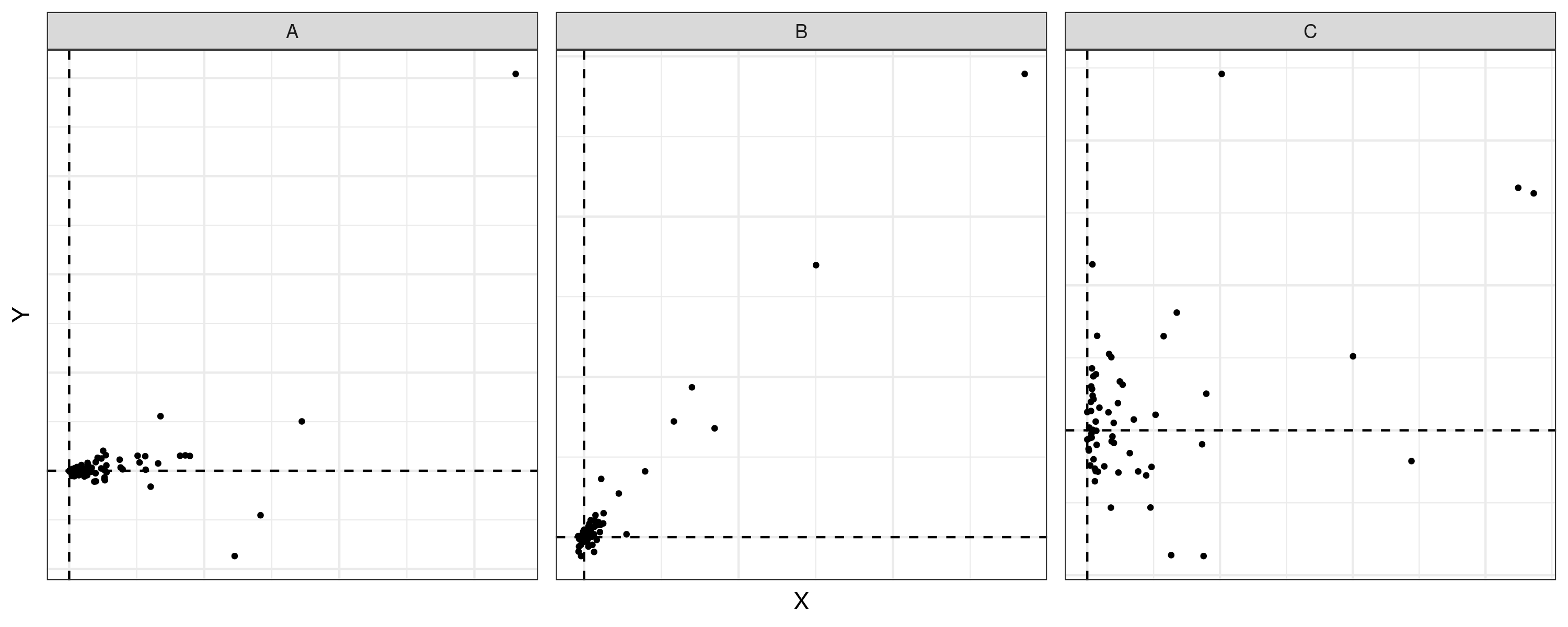
To illustrate the data heavy-tailedness, the scatter plots of for the three case studies are provided in Figure 2, where the scales of both and are removed in order to anonymize the experiments. In Table 4, we report the kurtosis as a measure of heavy-tailedness for the empirical distributions of
all of which are much larger than , which is the kurtosis of any univariate normal distribution.
| Case | Kurt() | Kurt() | Kurt() | |||||
|---|---|---|---|---|---|---|---|---|
| A | 30 | 80 | 80 | 2.79 | 0.84 | 1.09 | 1.00 | 0.22 |
| [-1.26, 5.69] | [0.23, 1.81] | [0.31, 1.85] | [0.25, 1.74] | |||||
| B | 50 | 40 | 10 | 1.00 | 0.81 | 0.87 | 1.00 | 0.00 |
| [0.81, 1.12] | [0.01, 1.06] | [0.56, 1.10] | [0.81, 1.12] | |||||
| C | 10 | 10 | 10 | 1.17 | 0.52 | 0.87 | 1.00 | 0.02 |
| [0.14, 2.18] | [-1.50, 2.69] | [-0.32, 1.97] | [-0.22, 1.94] |
Table 4 also lists the point estimates and confidence intervals for the empirical estimator , sign test based estimator , rank test based estimator , and Trimmed Match estimator . Here we see that and yield similar results except in experiment B, where the confidence interval from the rank based estimator is almost 74% wider than Trimmed Match. Meanwhile, the sign test based estimator gives confidence intervals that are even wider for all experiments by a considerable amount. It is also interesting to note that the data-driven choice of Trimmed Match’s trim rate results in no trimming (coinciding with the empirical estimator ) for case B despite the heavy-tailedness of the data, likely due to the approximately linear relationship between and (as shown in Figure 2) so that trimming a geo pair with a large may not necessarily reduce the variance. As experiment A demonstrates, however, the empirical estimator can sometimes be very unreliable as it is heavily affected by outliers (as shown in Figures 2 and 3).
Meanwhile, Figure 3 plots the Trimmed Match point estimate and confidence interval as a function of the trim rate . Here in case A, we note the significant reduction in the size of the confidence intervals relative to the empirical estimator , i.e. no trimming.

We also investigate whether the real data are incompatible with the statistical framework that we developed in Section 3 under Assumption Assumption 1, which assumes that the geo-level iROAS are all equal to one another. Recall from Proposition 2 that the distribution of the residuals is symmetric about 0, where is the number of geo pairs. Therefore, we expect to be approximately symmetric about 0 as well---a null hypothesis which we can test by using the Wilcoxon signed-rank test. The corresponding p-values44 4 Note that the p-values are based on the estimated (instead of the true values which are unknown) and thus may not be accurate. are 0.66, 0.55 and 0.85 for the above three real case studies, which suggest that the real data are not incompatible with Assumption Assumption 1. Figure 4 shows the boxplots of the fitted residuals for the three cases respectively, which illustrate the heavy-tailedness as well as approximate symmetry.

9 Discussion
In this paper, we introduced the iROAS estimation problem in online advertising and formulated a novel statistical framework for its causal inference in a randomized paired geo experiment design which is often complicated by the issues of small sample sizes, geo heterogeneity, and interference due to budgetary constraints on ad spend. Moreover, we proposed and developed a robust, distribution-free, and easily interpretable Trimmed Match estimator which adaptively trims poorly matched geo pairs. In addition, we devised a data-driven choice of the trim rate which extends Jaeckel’s idea but does not rely on asymptotic variance approximation, and presented numerical studies showing that Trimmed Match is often more efficient than alternative methods even when some of its assumptions are violated.
Several open research questions of considerable interest remain such as 1) using Trimmed Match to improve the design of matched pairs experiments, 2) using covariates to further improve the estimation precision (Rosenbaum 2002), 3) estimating the geo-level iROAS, and 4) further investigation of the choice of the trim rate and corresponding asymptotic analysis, e.g. using sample split (Klaassen 1987; Nie and Wager 2017).
Finally, although this paper focused on the estimation of the iROAS of online advertising in geo experiments, we note that Trimmed Match can also be applied to matched pairs experiments in other areas where the ratio of two causal estimands is of interest (e.g., the incremental cost-effectiveness ratio (Chaudhary and Stearns 1996; Bang and Zhao 2014); see Chapter 5.3 of Rosenbaum 2020 for more examples).
A Fast Computation of Trimmed Match
Recall from Section 5.1, that obtaining the Trimmed Match point estimate requires finding all roots of the trimmed mean equation (5.2). Moreover, recall that this computation is trivial when as just corresponds to the empirical estimator given by (1.3). Therefore, in the remainder of this section, we focus on the computation with a fixed trim rate .
Although (5.5) implies that calculating is straightforward once its corresponding set of untrimmed indices is known, is generally a priori unknown as it depends on . One could, at least in theory, check all possible subsets of size , but this brute force approach requires the evaluation of such subsets and would be computationally too expensive to be usable in practice when is large. However, by instead considering how the ordering of the values in the set changes as a function of —in particular, by enumerating all possible values of at which this ordering changes—we are able to devise an efficient algorithm for finding all of the roots of (5.2), which are required by (5.4).
Following (3.1), let be the differences in the ad spends and responses that are observed from a randomized paired geo experiment. For notational simplicity, assume that is ordered such that .
Lemma 2.
For any two pairs of geos and such that , let
Then if and only if .
Note that ties in rarely occur in practice; when ties do occur, they can be broken by adding a small amount of random noise to the ’s. Lemma 2, whose proof is straightforward and is omitted, allows us to efficiently solve the Trimmed Match equation defined by (5.2).
A.1 Solving the Trimmed Match Equation
For ease of exposition, assume that has been ordered such that , where . Then, for any , Lemma 2 implies that the ordering of is the same for all and, thus, the set of untrimmed indices
must also be the same for all . Moreover, Lemma 2 also implies that as increases and crosses a point , then for any , the ordering between and changes if and only if or .
Therefore, we can sequentially update the set of untrimmed indices based on what occurs as increases and crosses each point . If or if , then remains unchanged; if but , then we update by replacing with ; if but , then we update by replacing with . Pseudocode further describing this procedure is provided in Algorithm 1.
Input: and trim rate ; Let .
Output: roots of (5.2).
- i)
Reorder the pairs such that ; Calculate and order them such that . (Break ties with negligible random perturbation if needed.)
- ii)
Initialize the set of untrimmed indices with
Initialize , , and two ordered sets and .
- iii)
For :
- a)
If and , then update as follows:
and append to and to .
- b)
If and , then update , and similar to (a), and append to and to .
- c)
Otherwise, continue.
- a)
- iv)
Append to , and output a subset of as follows: For , output iff
A.2 Computing the Confidence Interval
A.3 Existence of
From our discussions in this section, it is not necessarily obvious whether the Trimmed Match point estimate always exists. However, the following theorem, whose proof is also omitted for conciseness, guarantees that it does indeed always exist as long as the trimmed mean of the ’s is nonzero.
Theorem 1.
(Existence) Suppose that is ordered such that . Then:
- 1)
is a continuous function with respect to .
- 2)
If , then has at least one root.
Acknowledgements
The authors would like to thank Art Owen and Jim Koehler for insightful early discussion, Peter Bickel for the reference of Jaeckel’s paper on the choice of trim rate, Nicolas Remy, Penny Chu and Tony Fagan for the support, Jouni Kerman, Yin-Hsiu Chen, Matthew Pearce, Fan Zhang, Jon Vaver, Susanna Makela, Kevin Benac, Marco Longfils and Christoph Best for interesting discussions, and the people who read and commented on the manuscript. We appreciate Editor Beth Ann Griffin and anonymous reviewers whose comments have helped improve the paper significantly. All the figures are produced with the R package ggplot2 (Wickham 2016).
References
- Angrist, Imbens and Rubin (1996) [author] Angrist, Joshua D.J. D., Imbens, Guido W.G. W. and Rubin, Donald B.D. B. (1996). Identification of causal effects using instrumental variables. Journal of the American statistical Association 91 444–455.
- Athey, Eckles and Imbens (2018) [author] Athey, SusanS., Eckles, DeanD. and Imbens, Guido W.G. W. (2018). Exact p-Values for Network Interference. Journal of the American Statistical Association 113 230-240.
- Baiocchi et al. (2010) [author] Baiocchi, MikeM., Small, Dylan S.D. S., Lorch, ScottS. and Rosenbaum, Paul R.P. R. (2010). Building a stronger instrument in an observational study of perinatal care for premature infants. Journal of the American Statistical Association 105 1285–1296.
- Bang and Zhao (2014) [author] Bang, HeejungH. and Zhao, HongweiH. (2014). Cost-effective analysis: a proposal of new reporting standards in statistical analysis. Journal of Biopharmaceutical Statistics 24 443 – 460.
- Blair and Kuse (2004) [author] Blair, Margaret HM. H. and Kuse, Allan RA. R. (2004). Better practices in advertising can change a cost of doing business to wise investments in the business. Journal of Advertising Research 44 71–89.
- Blake, Nosko and Tadelis (2015) [author] Blake, ThomasT., Nosko, ChrisC. and Tadelis, StevenS. (2015). Consumer Heterogeneity and Paid Search Effectiveness: A Large-Scale Field Experiment. Econometrica 83 155–174.
- Bloniarz et al. (2016) [author] Bloniarz, AdamA., Liu, HanzhongH., Zhang, Cun-HuiC.-H., Sekhon, Jasjeet S.J. S. and Yu, BinB. (2016). Lasso adjustments of treatment effect estimates in randomized experiments. Proceedings of the National Academy of Sciences 113 7383–7390.
- Brodersen et al. (2015) [author] Brodersen, Kay H.K. H., Gallusser, FabianF., Koehler, JimJ., Remy, NicolasN. and Scott, Steven L.S. L. (2015). Inferring causal impact using Bayesian structural time-series models. Annals of Applied Statistics 9 247–274.
- Interactive Advertising Bureau (2018) [author] Interactive Advertising Bureau (2018). IAB Internet Advertising Report: 2017 Full Year Results.
- Chaudhary and Stearns (1996) [author] Chaudhary, Mohammad A.M. A. and Stearns, Sally C.S. C. (1996). Estimating confidence intervals for cost-effectiveness ratios: an example from a randomized trial. Statistics in Medicine 15 1447–1458.
- Chen, Longfils and Best (2020) [author] Chen, AiyouA., Longfils, MarcoM. and Best, ChristophC. (2020). The Python library for Trimmed Match and Trimmed Match Design. https://github.com/google/trimmed_match. [Online; accessed 21-April-2021].
- Chen et al. (2018) [author] Chen, AiyouA., Chan, DavidD., Perry, MikeM., Jin, YuxueY., Sun, YuntingY., Wang, YueqingY. and Koehler, JimJ. (2018). Bias correction for paid search in media mix modeling Technical Report, Google Inc. https://ai.google/research/pubs/pub46861.
- Dhar and Chaudhuri (2012) [author] Dhar, Subhra SankarS. S. and Chaudhuri, ProbalP. (2012). On the derivatives of the trimmed mean. Statistica Sinica 22 655–679.
- Ding, Feller and Miratrix (2016) [author] Ding, PengP., Feller, AviA. and Miratrix, LukeL. (2016). Randomization inference for treatment effect variation. Journal of the Royal Statistical Society: Series B 78 655–671.
- Goldfarb and Tucker (2011) [author] Goldfarb, AviA. and Tucker, CatherineC. (2011). Online Advertising. In Advances in Computers, (Marvin V.M. V. Zelkowitz, ed.) 81 6, 289–315. Elsevier.
- Gordon et al. (2019) [author] Gordon, BrettB., Zettelmeyer, FlorianF., Bhargava, NehaN. and Chapsky, DanD. (2019). A Comparison of Approaches to Advertising Measurement: Evidence from Big Field Experiments at Facebook. Marketing Science 38 193–225.
- Hall (1981) [author] Hall, PeterP. (1981). Large sample properties of Jaeckel’s adaptive trimmed mean. Annals of the Institute of Statistical Mathematics 33 449–462.
- Huber and Ronchetti (2009) [author] Huber, Peter J.P. J. and Ronchetti, ElvezioE. (2009). Robust statistics. John Wiley & Sons, Inc.
- Hudgens and Halloran (2008) [author] Hudgens, Michael GM. G. and Halloran, M ElizabethM. E. (2008). Toward causal inference with interference. Journal of the American Statistical Association 103 832–842.
- Imbens and Rubin (2015) [author] Imbens, Guido W.G. W. and Rubin, Donald B.D. B. (2015). Causal Inference for Statistics, Social, and Biomedical Sciences: An Introduction. Cambridge University Press, New York, NY, USA.
- Jaeckel (1971) [author] Jaeckel, Louis A.L. A. (1971). Some flexible estimates of location. The Annals of Mathematical Statistics 42 1540–1552.
- Johnson, Lewis and Nubbemeyer (2017) [author] Johnson, Garrett A.G. A., Lewis, Randall A.R. A. and Nubbemeyer, Elmar I.E. I. (2017). Ghost ads: Improving the economics of measuring online ad effectiveness. Journal of Marketing Research 54 867–884.
- Kalyanam et al. (2018) [author] Kalyanam, KirthiK., McAteer, JohnJ., Marek, JonathanJ., Hodges, JamesJ. and Lin, LifengL. (2018). Cross channel effects of search engine advertising on brick & mortar retail sales: Meta analysis of large scale field experiments on Google.com. Quantitative Marketing and Economics 16 1–42.
- Kerman, Wang and Vaver (2017) [author] Kerman, JouniJ., Wang, PengP. and Vaver, JonJ. (2017). Estimating Ad Effectiveness using Geo Experiments in a Time-Based Regression Framework Technical Report, Google, Inc. https://ai.google/research/pubs/pub45950.
- Klaassen (1987) [author] Klaassen, Chris AJC. A. (1987). Consistent estimation of the influence function of locally asymptotically linear estimators. The Annals of Statistics 1548–1562.
- Kunzel et al. (2019) [author] Kunzel, Soren R.S. R., Sekhon, Jasjeet S.J. S., Bickel, Peter J.P. J. and Yu, BinB. (2019). Metalearners for estimating heterogeneous treatment effects using machine learning. Proceedings of the National Academy of Sciences 116 4156–4165.
- Lehmann (2006) [author] Lehmann, Erich LeoE. L. (2006). Nonparametrics: statistical methods based on ranks. Springer.
- Lewis and Rao (2015) [author] Lewis, Randall A.R. A. and Rao, Justin M.J. M. (2015). The Unfavorable Economics of Measuring the Returns to Advertising. The Quarterly Journal of Economics 130 1941-1973.
- Lin (2013) [author] Lin, WinstonW. (2013). Agnostic notes on regression adjustments to experimental data: Reexamining Freedman’s critique. The Annals of Applied Statistics 7 295–318.
- Luo et al. (2012) [author] Luo, XiX., Small, Dylan S.D. S., Li, Chiang-Shan R.C.-S. R. and Rosenbaum, Paul R.P. R. (2012). Inference With Interference Between Units in an fMRI Experiment of Motor Inhibition. Journal of the American Statistical Association 107 530-541.
- Nie and Wager (2017) [author] Nie, XinkunX. and Wager, StefanS. (2017). Quasi-oracle estimation of heterogeneous treatment effects. arXiv preprint arXiv:1712.04912.
- Rolnick et al. (2019) Rolnick, D., Aydin, K., Pouget-Abadie, J., Kamali, S., Mirrokni, V. and Najmi, A. (2019). Randomized Experimental Design via Geographic Clustering. In Proceedings of the 25th ACM International Conference on Knowledge Discovery & Data Mining 2745–2753. https://doi.org/10.1145/3292500.3330778
- Rosenbaum (1996) [author] Rosenbaum, Paul R.P. R. (1996). Identification of causal effects using instrumental variables: Comment. Journal of the American Statistical Association 91 444–444.
- Rosenbaum (2002) [author] Rosenbaum, Paul R.P. R. (2002). Covariance adjustment in randomized experiments and observational studies. Statistical Science 17 286–327.
- Rosenbaum (2007) [author] Rosenbaum, Paul RP. R. (2007). Interference Between Units in Randomized Experiments. Journal of the American Statistical Association 102 191-200.
- Rosenbaum (2020) [author] Rosenbaum, Paul R.P. R. (2020). Design of Observational Studies, 2nd Edition. Springer Series in Statistics.
- Rubin (1980) [author] Rubin, Donald B.D. B. (1980). Discussion of "Randomization Analysis of Experimental Data in the Fisher Randomization Test" by Basu. Journal of the American Statistical Association 75 591-593.
- Sapp et al. (2017) [author] Sapp, StephanieS., Vaver, JonJ., Schuringa, JonJ. and Dropsho, StevenS. (2017). Near impressions for observational causal ad impact Technical Report, Google Inc. https://ai.google/research/pubs/pub46418.
- Small and Rosenbaum (2008) [author] Small, DylanD. and Rosenbaum, Paul R.P. R. (2008). War and Wages: The Strength of Instrumental Variables and Their Sensitivity to Unobserved Biases. Journal of the American Statistical Association 103 924-933.
- Tukey and McLaughlin (1963) [author] Tukey, John W.J. W. and McLaughlin, Donald H.D. H. (1963). Less vulnerable confidence and significance procedures for location based on a single sample: Trimming/Winsorization 1. Sankhyā: The Indian Journal of Statistics, Series A 25 331–352.
- Varian (2009) [author] Varian, Hal R.H. R. (2009). Online Ad Auctions. American Economic Review 99 430-34. 10.1257/aer.99.2.430
- Varian (2016) [author] Varian, Hal R.H. R. (2016). Causal inference in economics and marketing. Proceedings of the National Academy of Sciences 113 7310–7315.
- Vaver and Koehler (2011) [author] Vaver, JonJ. and Koehler, JimJ. (2011). Measuring Ad Effectiveness Using Geo Experiments Technical Report, Google Inc. https://ai.google/research/pubs/pub38355.
- Wager and Athey (2018) [author] Wager, StefanS. and Athey, SusanS. (2018). Estimation and Inference of Heterogeneous Treatment Effects using Random Forests. Journal of the American Statistical Association 113 1228-1242. 10.1080/01621459.2017.1319839
- Wickham (2016) [author] Wickham, HadleyH. (2016). ggplot2: Elegant Graphics for Data Analysis. Springer-Verlag New York.
- Ye et al. (2016) Ye, Q., Malik, S., Chen, J. and Zhu, H. (2016). The Seasonality Of Paid Search Effectiveness From A Long Running Field Test. In Proceedings of the 2016 ACM Conference on Economics and Computation. EC ’16 515–530. ACM, New York, NY, USA.