Time- and momentum-resolved phonon population dynamics
with ultrafast electron diffuse scattering

UEDS measurements are pump-probe experiments in which an ultrafast laser pulse is used to photoexcite a thin single-crystal specimen at $t=t_{0}$, followed by probing the specimen with an ultrafast electron pulse at $t=t_{0}+\tau$, resulting in the acquisition of a transmission electron scattering pattern. By scanning across time-delays $\tau$, the dynamics in the $\mathrm{fs}$ – $\mathrm{ns}$ ($10^{-15}\textrm{--}10^{-9}$ $\mathrm{s}$) range can be recorded. UEDS data can be acquired coincidentally during ultrafast electron diffraction (UED) experiments with state-of-the-art detection cameras, although UEDS intensities are empirically $10^{4}$ to $10^{6}$ times less intense than those of Bragg diffraction. UEDS measurements are inherently statistical. Pump-probe experiments sample many decay processes, incoherently in time. Hence, all possible decay channels are represented, proportionally to their statistical likelihood.

Scattering measurements presented in this work use bunches of $10^{7}$ electrons, accelerated to $90\text{\,}\mathrm{keV}$, at a repetition rate of $1\text{\,}\mathrm{kHz}$. A radio-frequency cavity is used to compress electron bunches to $\approx$150\text{\,}\mathrm{fs}$$ at the sample, as measured by a home-built photoactivated streak camera Kassier et al. 2010. More detailed descriptions of this instrument are given elsewhere Chatelain et al. 2012; Morrison et al. 2013; Otto et al. 2017. Analysis of static diffraction patterns indicate a momentum resolution of $0.06\text{\,}{\mathrm{\SIUnitSymbolAngstrom}}^{-1}$, while the range of visible reflections is consistent with a real-space resolution of $<$1\text{\,}\mathrm{\SIUnitSymbolAngstrom}$$. $35\text{\,}\mathrm{fs}$ pump laser pulses of $800\text{\,}\mathrm{nm}$ ($1.55\text{\,}\mathrm{eV}$) light are used to photoexcite a single-crystal flake of freestanding single crystal natural graphite, provided by Naturally Graphite. The flakes were mechanically exfoliated to a thickness of $70\text{\,}\mathrm{nm}$.

The interrogated film area covers $500\text{\times}500\text{\,}\mathrm{\SIUnitSymbolMicro m}$, with a pump spot of $1\text{\times}1\text{\,}\mathrm{mm}$ full-width half-max (FWHM) ensuring nearly uniform illumination of the probed volume. The film was pumped at a fluence of $12\text{\,}\mathrm{mJ}\text{\,}{\mathrm{cm}}^{-2}$, resulting in an absorbed energy density of $8\text{\,}\mathrm{J}\text{\,}{\mathrm{m}}^{-3}$. The scattering patterns are collected with a Gatan Ultrascan 895 camera; a $2.54\text{\times}2.54\text{\,}\mathrm{cm}$ phosphor screen fiber-coupled to a $2048\text{\times}2048\text{\,}\mathrm{p}\mathrm{x}$ charge-coupled detector (CCD) placed $25\text{\,}\mathrm{cm}$ away from the sample. The experiment herein consists of time-delays in the range of $-40\text{\,}\mathrm{ps}680\text{\,}\mathrm{ps}$. Per-pixel scattering intensity fluctuations over laboratory time reveals a transient dynamic range of $1:10^{8}$, allowing the acquisition of diffraction patterns and diffuse scattering patterns simultaneously ¹¹ 1 The intensity fluctuations of pixel values across scattering patterns acquired before photoexcitation are $10^{8}$ times smaller than the brightest Bragg reflection.

Scattering intensity patterns are inherently redundant due to the point-group symmetry of the scattering crystal. When this symmetry is not broken by photoexcitation or the dynamical phenomena itself, it is possible to use this redundancy to enhance the signal to noise ratio of a UEDS data set. No dynamical phenomena breaking point-group symmetry was observable within the raw signal to noise of the current measurements, so the measured patterns have been subject to a six-fold discrete azimuthal average based on the $D_{6h}$ point-group of graphite. This discrete rotational average effectively increases the signal-to-noise ratio of this data set by a factor of $\sqrt{6}$ and is therefore an effective data processing step given the weakness of the diffuse scattering signals. “Scattering intensities” is henceforth implied to mean six-fold averaged scattering intensities.

Scattering from a few samples with varying thicknesses ($10\text{\,}\mathrm{nm}90\text{\,}\mathrm{nm}$) was acquired. There was no quantitative difference in the Bragg scattering dynamics, indicating that scattering from these samples is kinematical to a good approximation. The expected effects of multiple scattering on the diffuse scattering intensity distribution will be discussed further below.

Structure relaxation was performed using the plane-wave self-consistent field program PWscf from the Quantum ESPRESSO software suite Giannozzi et al. 2017. The graphite structure was fully relaxed using a $18\text{\times}18\text{\times}10$ $\bm{\mathrm{k}}$-point mesh centered at $\bm{\mathrm{\Gamma}}$ and force (energy) threshold of $1\text{\times}{10}^{-8}\text{\,}\mathrm{R}\mathrm{y}\mathrm{/}\mathrm{B}\mathrm{o}\mathrm{h}\mathrm{r}$ ($1\text{\times}{10}^{-14}\text{\,}\mathrm{R}\mathrm{y}$). The dynamical matrices were computed on $5\text{\times}3\text{\times}3$ $\bm{\mathrm{q}}$-point grid using a self-consistency threshold of $1\text{\times}{10}^{-18}\text{\,}\mathrm{R}\mathrm{y}$. The resulting graphite structure has the following lattice vectors:

where $a=$2.462\text{\,}\mathrm{\SIUnitSymbolAngstrom}$$, $c=$6.837\text{\,}\mathrm{\SIUnitSymbolAngstrom}$$, and $\left\{\bm{\mathrm{e}}_{i}\right\}$ are the usual Euclidean vectors. Graphite has four atoms in the unit cell, with two groups of two atoms forming lattices rotated with respect to each other. This structure respects the symmetries of the $D_{6h}$ point group ²² 2 The space group of this structure is $P6_{3}/mmc$ (Hermann-Mauguin symbol) or $D_{6h}^{4}$ (Schoenflies symbol)..

The phonon frequencies $\left\{\omega_{j,\bm{\mathrm{k}}}\right\}$ and polarization vectors $\left\{\bm{\mathrm{e}}_{j,s,\bm{\mathrm{k}}}\right\}$ were computed using the PHonon program in the Quantum ESPRESSO software suite, using the B86b exchange-coupled Perdew-Burke-Ernzerhof (B86bPBE) generalized gradient approximation (GGA) and the projector augmented-wave (PAW) method Becke 1986; Perdew et al. 1996; Blöchl 1994. The cutoff-energy of the wavefunction was set to $100\text{\,}\mathrm{R}\mathrm{y}$, while the cutoff energy for the charge density was set to $1200\text{\,}\mathrm{R}\mathrm{y}$, and a Fermi-Dirac smearing of $0.06\text{\,}\mathrm{R}\mathrm{y}$ was applied. To include the dispersion energy between the carbon layers, the exchange-hole dipole moment (XDM) method was used Becke and Johnson 2007.

The quantitative connection between the observed diffuse intensity $I_{1}(\bm{\mathrm{q}},t)$ and the phonon populations, $\left\{n_{j,\bm{\mathrm{k}}}\right\}$, is provided by the one-phonon structure factors, $|F_{1j}(\bm{\mathrm{q}},t)|^{2}$. A determination of $|F_{1j}(\bm{\mathrm{q}},t)|^{2}$ requires phonon polarization vectors $\left\{\bm{\mathrm{e}}_{j,s,\bm{\mathrm{k}}}\right\}$ and associated frequencies $\left\{\omega_{j,\bm{\mathrm{k}}}\right\}$. Density functional perturbation theory (DFPT) is a widely used, readily-available method to compute these phonon properties.

The separation of frequencies and polarization vectors into modes is key to the calculation of one-phonon structure factors $|F_{1j}(\bm{\mathrm{q}},t)|^{2}$. The phonon frequencies $\left\{\omega_{j,\bm{\mathrm{k}}}\right\}$ and polarization vectors $\left\{\bm{\mathrm{e}}_{j,s,\bm{\mathrm{k}}}\right\}$ were computed independently at every $\bm{\mathrm{k}}$; however, diagonalization routines have no way of clustering eigenvalues and eigenvectors into physically-relevant groups (i.e. phonon branches). Association between atomic motions (given by polarization vectors) and a particular mode is only well-defined near the $\bm{\mathrm{\Gamma}}$-point Paulatto et al. 2013. Clustering of phonon properties into phonon branches is described in detail in Appendix A.

The polarization vectors and frequencies, calculated for irreducible $\bm{\mathrm{k}}$-points ⁴⁴ 4 The coverage of irreducible $\bm{\mathrm{k}}$-points is important. Only computing phonon properties along high-symmetry lines is fraught with peril, given that polarization vectors can vary significantly not only along high-symmetry lines, but over the entire Brillouin zone., were extended over the entire reciprocal space based on crystal symmetries using the crystals software package René de Cotret et al. 2018.

A key component of the computation of one-phonon structure factors $|F_{1j}(\bm{\mathrm{q}},t)|^{2}$ is the calculation of the Debye-Waller factors $\left\{W_{s}(\bm{\mathrm{q}},t)\right\}$, representing the instantaneous disorder of the material. Based on Equation (4), terms of the form $\left\{W_{s}(\bm{\mathrm{q}},t)\right\}$ are not sensitive reporters on the wavevector dependence of nonequilibrium phonon distributions because their value at every $\bm{\mathrm{q}}$ involves a sum of all mode, at every reduced wavevector $\bm{\mathrm{k}}$. Phonon population dynamics can only affect the magnitude of the Debye-Waller factors. The potential time dependence of the Debye-Waller factors was investigated, via the time dependence of mode populations $\left\{n_{j,\bm{\mathrm{k}}}\right\}$. Profoundly non-equilibrium distributions of phonon modes were simulated, with all modes populated equivalently to a temperature of $300\text{\,}\mathrm{K}$ except one mode at high temperature ⁵⁵ 5 A maximum of $5000\text{\,}\mathrm{K}$ for optical modes, and $1000\text{\,}\mathrm{K}$ for acoustic modes. The discrepancy between maximum temperatures represents the fact that the heat capacity of acoustic modes is much higher.. These extreme non-equilibrium distributions increased the value the terms $\sum_{s}W_{s}(\bm{\mathrm{q}},t)$ by at most $1.5\text{\,}\mathrm{\%}$ for optical modes, and $5\text{\,}\mathrm{\%}$ for acoustic modes. Since these fractional changes are constant across $\bm{\mathrm{q}}$, wavevector-dependent changes in UEDS signals are not impacted significantly by transient changes to the Debye-Waller factors and any time dependence of the one-phonon structure factors $|F_{1j}(\bm{\mathrm{q}},t)|^{2}$ that result from the Debye-Waller factors themselves can be ignored to a good approximation.

Using the computed Debye-Waller factors from the previous section, the calculation of $|F_{1j}(\bm{\mathrm{q}},t)|^{2}$ was carried out, from Equation (3), for the eight in-plane phonon modes of graphite: the longitudinal modes LA, LO1 -- LO3, and the transverse modes TA, TO1 -- TO3 ⁶⁶ 6 The calculation of $|F_{1j}(\bm{\mathrm{q}},t)|$ is trivial for out-of-plane modes ZA, ZO1 – ZO3 because $\bm{\mathrm{q}}\cdot\bm{\mathrm{e}}_{j,s,\bm{\mathrm{k}}}\equiv 0$ for these modes.. The resulting one-phonon structure factors of a few in-plane modes, with occupations equivalent to a temperature of $300\text{\,}\mathrm{K}$, are shown in Figure 3. One-phonon structure factors $|F_{1j}(\bm{\mathrm{q}},t)|^{2}$ display striking scattering vector dependence (selection rules) based on the nature of phonon polarization vectors $\left\{\bm{\mathrm{e}}_{j,s,\bm{\mathrm{k}}}\right\}$. Specifically, near $\bm{\mathrm{\Gamma}}$, the one-phonon structure factor for longitudinal modes is highest in the radial direction, because the polarization of those modes is parallel to $\bm{\mathrm{q}}$. On the other hand, $|F_{1j}(\bm{\mathrm{q}},t)|^{2}$ for transverse modes is highest (near $\bm{\mathrm{\Gamma}}$) in the azimuthal direction for transverse modes, because the polarization of those modes is perpendicular to $\bm{\mathrm{q}}$.

An alternative view of one-phonon structure factors is presented via weighted dispersion curves, an example of which is shown in Figure 4. This presentation allows easy comparison of the relative weights of the one-phonon structure factors along high-symmetry lines for different phonon branches.

A cursory inspection of the weighted dispersion curves in Figure 4 suggest that there are regions in the Brillouin zone where diffuse intensity is strongly biased towards a single mode (strong scattering selection rule) based on the relative intensities of one-phonon structure factors. Careful analysis reveals that there are very few wavevectors $\bm{\mathrm{q}}$ for which a particular phonon mode’s one-phonon structure factor is strongly dominant. Figure 5 presents a comparison of the relative intensities of one-phonon structure factors weighted by phonon frequency, which is indicative of mode population as per Equation (2). Only $37\%$ of wavevectors visible in measurements shown in Figure 2 have a mode that contributes over $50\%$ of the quantity $\sum_{j}|F_{1j}(\bm{\mathrm{q}})|^{2}/\omega_{j,\bm{\mathrm{k}}}$; only $1\%$ of wavevectors have a phonon mode that contributes more than $75\%$.

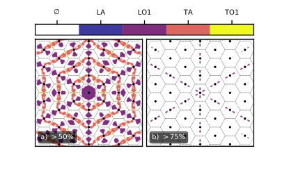
The results of Figure 5 show that quantitative answers regarding phonon dynamics from UEDS measurements cannot generally be obtained by inspection; at almost any wavevector $\bm{\mathrm{q}}$, at least two phonon modes contribute significantly to the transient diffuse scattering intensity. Therefore, a more robust procedure, presented in the next section, must be employed to extract wavevector- anndmode-dependent phonon populations from UEDS intensities.

Transient electron diffuse intensity has been used elsewhere Chase et al. 2016; Waldecker et al. 2017; Stern et al. 2018; Konstantinova et al. 2018 as an approximation to the population dynamics of particular modes. However, one can extract the transient wavevector-dependent phonon population dynamics $\left\{\Delta n_{j,\bm{\mathrm{k}}}(t)\right\}$ by combining the measurements of $\Delta I(\bm{\mathrm{q}},t)$ with the calculations of one-phonon structure factors and associated quantities presented above.

For many materials (including graphite), the temperature dependence (and hence time dependence) of the phonon mode vibrational frequencies is negligible, because such dependence is proportional to anharmonic couplings between branches Calizo et al. 2007; Judek et al. 2015; hence, $\omega_{j,\bm{\mathrm{k}}}(t)\equiv\omega_{j,\bm{\mathrm{k}}}(t_{0})$. Moreover, as is discussed in Section IV.2, the temperature dependence (and hence time dependence) of the Debye-Waller factors — and therefore the one-phonon structure factors — has a much smaller magnitude that the variations due to other terms in Equation (2). Therefore, we have $|F_{1j}(\bm{\mathrm{q}},t)|^{2}\equiv|F_{1j}(\bm{\mathrm{q}},t_{0})|^{2}$ for all times. In this case, transient scattering intensity at the detector, $\Delta I(\bm{\mathrm{q}},t)$, can be expressed as follows:

for $\bm{\mathrm{k}}$ away from $\bm{\mathrm{\Gamma}}$, where there might be interference with elastic scattering signals.

At every reduced wavevector $\bm{\mathrm{k}}$ and time-delay $t$, there are $N$ different values $\left\{\Delta n_{j,\bm{\mathrm{k}}}(t)\right\}$ that must be determined — one for each phonon mode. Since the one-phonon structure factors $|F_{1j}(\bm{\mathrm{q}},t_{0})|^{2}$ vary over the total wavevector $\bm{\mathrm{q}}$, the transient diffuse intensity for at least $N$ Brillouin zones must be considered so that Equation (6) can be solved numerically. A linear system of equations must be solved at every reduced wavevector $\bm{\mathrm{k}}$.

Let $\{\bm{\mathrm{H}}_{1},...,\bm{\mathrm{H}}_{M}\mid M\geq N\}$ be the chosen reflections from which to build the system of equations. Then, the transient phonon population of mode $j$ at every $\bm{\mathrm{k}}$ and time $t$, $\Delta n_{j,\bm{\mathrm{k}}}(t)$, solves the linear system:

where

for $\bm{\mathrm{k}}$ vectors away from the $\bm{\mathrm{\Gamma}}$ point. These linear systems of equations can be solved numerically, provided enough experimental data ($M\geq N$).

The choice to solve for $\bm{\mathrm{n}}_{\bm{\mathrm{k}}}(t)$, rather than for the change in population, is related to the degree of confidence that should be placed in the calculation of phonon polarization vectors and frequencies. The phonon polarization vectors are mostly affected by the symmetries of the crystal. On the other hand, phonon vibrational frequencies might be influenced by non-equilibrium carrier distributions. Solving for the ratio of populations to frequencies, rather than populations, is more robust against the uncertainty in the modelling, because the one-phonon structure factors only take into account the polarization vectors.

We also note that the procedure presented above can be easily extended to (equilibrium) thermal diffuse scattering measurements, where the phonon populations are known at constant temperature, but the phonon vibrational spectrum is unknown. Therefore, using pre-photoexcitation data of a time-resolved experiment, one could infer the phonon vibrational frequencies, which are then used to determine the change in populations using the measurements after photoexcitation. This scheme only relies on the determination of phonon polarization vectors.

The flow of energy between electronic and phononic subsystems is typically crudely modelled using the two-temperature model Allen 1987. This model assumes that the electronic system and the phononic system can each be associated with temperatures $T_{e}$ and $T_{ph}$, throughout the dynamics. Effectively this approximation assumes that the internal thermalization dynamics of each system is much more rapid than any processes that couple the two system. It is evident from the earlier description of the UEDS data from graphite that this assumption is (rather generally) quite a poor one; the idea that the phononic subsystem is internally thermalized does not hold on the timescales typically associated with energy flows between the electron and phonon systems following photoexcitation. On these timescales the phonon occupations are generally very far from being thermalized. UEDS allows to move beyond the two-temperature approximation; by leveraging momentum-resolution, mode-dependent electron-phonon and phonon-phonon couplings can be extracted from the transient change in mode populations $\left\{\Delta n_{j,\bm{\mathrm{k}}}(t)\right\}$. Specifically, wavevector-dependent phonon population dynamics determined in the previous section will now be used to determine the electron-phonon and phonon-phonon coupling strength of the $A_{1}^{\prime}$ phonon.

The formalism of the two-temperature model can be extended to the non-thermal lattice model (NLM) model Waldecker et al. 2016, where every phonon branch $j$ has its own molar heat capacity $C_{ph,j}$, and temperature $T_{ph,j}$:

where $f(t-t_{0})$ is the laser pulse profile, and $C_{e}$ and $T_{e}$ are the electronic heat capacity and electron temperature, respectively ⁹⁹ 9 The electronic system thermalizes in approximately $100\text{\,}\mathrm{fs}$ Stange et al. 2015, and hence after we can consider the electronic system to be well-described by a single temperature $T_{e}$.. This model accounts for discrepancies in coupling between the electronic system and certain phonon modes, which occurs for example in graphite — where some modes are strongly-coupled to the electron system via Kohn anomalies Piscanec et al. 2004.

Observations of transient changes in mode populations are related to mode temperatures $T_{ph,j}(t)$ via the Bose-Einstein distribution:

We can decompose the above expression with a Laurent series Wunsch 2005 to show explicitly that the mode population is proportional to temperature, for appropriately high $T_{ph,j}$:

Hence, in the case of measurements presented herein, $\Delta n_{j,\bm{\mathrm{k}}}(t)\propto\Delta T_{ph,j}(t)$, where the initial temperature is known to be $300\text{\,}\mathrm{K}$.

We now use the NLM to extract the couplings to the $A_{1}^{\prime}$ mode from population measurements. The differential $A_{1}^{\prime}$ phonon population $\Delta n_{A_{1}^{\prime}}(t)$ is obtained by integrating over the region of the wavevector-dependent TO2 phonon population, in a circular arc centered at $\bm{\mathrm{K}}$ ($|\bm{\mathrm{k}}-\bm{\mathrm{K}}|\leq$0.3\text{\,}{\mathrm{\SIUnitSymbolAngstrom}}^{-1}$$). This location is shown in Figure 6. In order to correlate the mode population measurements with the NLM, the heat capacities of the electronic system and every phonon mode must be parametrized.

The electronic heat capacity $C_{e}$ is extracted from experimental work by Nihira and Iwata 2003:

Over this range of time-delays, thermal expansion (or contraction, in the case of graphite) has not yet occurred Chatelain et al. 2014. No changes in Bragg peak positions — indicative of lattice parameter changes — is observed within the experimental range of time-delays $\tau\leq$680\text{\,}\mathrm{ps}$$. We can therefore calculate the heat capacity of each graphite mode $j$ as the heat capacity at constant volume Ziman 1979:

where $k_{B}$ is the Boltzmann constant, $\omega_{D}$ is the Debye frequency, and $D(\omega)$ is the phonon density of states. Momentum resolution of UEDS allows for a simplification, where a single frequency contributes to the heat capacity in the $A_{1}^{\prime}$ mode — $D(\omega)=\delta(\omega)$. Moreover, we can reduce the number of coupled equations in Equations (11) and (12). Simultaneous conservation of momentum and energy during the decay of an $A_{1}^{\prime}$ phonon can only be satisfied in a few reciprocal space locations. Using first-principles calculations, it is possible to determine the decay probabilities. One such calculation, reported by Bonini et al. 2007, allows us to define an effective heat capacity into which the $A_{1}^{\prime}$ population drains, $C_{l}$ ¹⁰¹⁰ 10 This effective heat capacity $C_{l}$ is composed of 9% chance to decay into two TA modes, 36% change to decay into a TA mode and an LA mode, and 55% chance to decay into either an LA and TA, or LO and LA.. Therefore, the energy dynamics at $\bm{\mathrm{K}}$ can be specified in terms of a system of three equations:

where $G_{e,A_{1}^{\prime}}$, $G_{A_{1}^{\prime},l}$, and $G_{e,l}$ are constants. Solving this system of equations gives the temperature evolution of each of the subsystems. The evolution in the $A_{1}^{\prime}$ population can be used as a proxy for the mode temperature $T_{A_{1}^{\prime}}(t)$; minimizing the difference between observed population dynamics and modelled temperature changes yields the coupling constants $G_{e,A_{1}^{\prime}}$, $G_{A_{1}^{\prime},l}$, and $G_{e,l}$. The resulting temperature transients are presented in Figure 7. The extracted coupling constants have been listed in Table 1. This model correctly identifies the strong electron-phonon coupling of the $A_{1}^{\prime}$ mode, $G_{e,A_{1}^{\prime}}$, as compared with the rest of the relevant modes, $G_{e,l}$.

From the coupling constant $G_{e,A_{1}^{\prime}}$, mode-projected electron-phonon coupling value $\langle g_{e,A_{1}^{\prime}}^{2}\rangle$ can be determined. In the case of the coupling between the electron system and the $A_{1}^{\prime}$ phonon, the heating rate of $G_{e,A_{1}^{\prime}}=$6.8\pm\pm 0.3\text{\times}{10}^{17}\text{\,}\mathrm{W}\text{\,}{\mathrm{m}}^{-3}\text{\,}{\mathrm{K}}^{-1}$$ (Table 1) corresponds to a mode-projected electron-phonon coupling value of $\langle g_{e,A_{1}^{\prime}}^{2}\rangle=$0.035\pm\pm 0.001\text{\,}{\mathrm{eV}}^{2}$$ (see appendix B for details). These values are in agreement with recent trARPES measurements and simulations Johannsen et al. 2013; Stange et al. 2015; Rohde et al. 2018; Na et al. 2019.

References

- Eliashberg (1960) G. Eliashberg, Interactions between electrons and lattice vibrations in a superconductor, Sov. Phys. JETP 11, 696 (1960).
- Hur et al. (2004) N. Hur, S. Park, P. Sharma, J. Ahn, S. Guha, and S.-W. Cheong, Electric polarization reversal and memory in a multiferroic material induced by magnetic fields, Nature 429, 392 (2004).
- Zhao et al. (2016) L.-D. Zhao, G. Tan, S. Hao, J. He, Y. Pei, H. Chi, H. Wang, S. Gong, H. Xu, V. P. Dravid, C. Uher, G. J. Snyder, C. Wolverton, and M. G. Kanatzidis, Ultrahigh power factor and thermoelectric performance in hole-doped single-crystal snse, Science 351, 141 (2016).
- Miyata et al. (2017) K. Miyata, D. Meggiolaro, M. T. Trinh, P. P. Joshi, E. Mosconi, S. C. Jones, F. De Angelis, and X.-Y. Zhu, Large polarons in lead halide perovskites, Science Advances 3, 10.1126/sciadv.1701217 (2017).
- Kim et al. (2012) K. W. Kim, A. Pashkin, H. Schäfer, M. Beyer, M. Porer, T. Wolf, C. Bernhard, J. Demsar, R. Huber, and A. Leitenstorfer, Ultrafast transient generation of spin-density-wave order in the normal state of bafe 2 as 2 driven by coherent lattice vibrations, Nature materials 11, 497 (2012).
- Lanzara et al. (2001) A. Lanzara, P. Bogdanov, X. Zhou, S. Kellar, D. Feng, E. Lu, T. Yoshida, H. Eisaki, A. Fujimori, K. Kishio, et al., Evidence for ubiquitous strong electron–phonon coupling in high-temperature superconductors, Nature 412, 510 (2001).
- Lan et al. (2019) Y. Lan, B. J. Dringoli, D. A. Valverde-Chávez, C. S. Ponseca, M. Sutton, Y. He, M. G. Kanatzidis, and D. G. Cooke, Ultrafast correlated charge and lattice motion in a hybrid metal halide perovskite, Science Advances 5 (2019).
- Porer et al. (2014) M. Porer, U. Leierseder, J.-M. Ménard, H. Dachraoui, L. Mouchliadis, I. E. Perakis, U. Heinzmann, J. Demsar, K. Rossnagel, and R. Huber, Non-thermal separation of electronic and structural orders in a persisting charge density wave, Nature Materials 13, 857 (2014).
- Tsen and Ferry (2009) K. T. Tsen and D. K. Ferry, Studies of electron–phonon and phonon–phonon interactions in InN using ultrafast Raman spectroscopy, Journal of Physics: Condensed Matter 21, 174202 (2009).
- Yan et al. (2009) H. Yan, D. Song, K. F. Mak, I. Chatzakis, J. Maultzsch, and T. F. Heinz, Time-resolved Raman spectroscopy of optical phonons in graphite: Phonon anharmonic coupling and anomalous stiffening, Physical Review B 80, 121403(R) (2009).
- Yang et al. (2017) J.-A. Yang, S. Parham, D. Dessau, and D. Reznik, Novel Electron-Phonon Relaxation Pathway in Graphite Revealed by Time-Resolved Raman Scattering and Angle-Resolved Photoemission Spectroscopy, Scientific Reports 7, 40876 (2017).
- Johannsen et al. (2013) J. C. Johannsen, S. Ulstrup, F. Cilento, A. Crepaldi, M. Zacchigna, C. Cacho, I. C. E. Turcu, E. Springate, F. Fromm, C. Raidel, T. Seyller, F. Parmigiani, M. Grioni, and P. Hofmann, Direct View of Hot Carrier Dynamics in Graphene, Physical Review Letters 111, 027403 (2013).
- Gierz et al. (2015) I. Gierz, F. Calegari, S. Aeschlimann, M. C. Cervantes, C. Cacho, R. T. Chapman, E. Springate, S. Link, U. Starke, C. R. Ast, and A. Cavalleri, Tracking Primary Thermalization Events in Graphene with Photoemission at Extreme Time Scales, Physical Review Letters 115, 086803 (2015).
- Stange et al. (2015) A. Stange, C. Sohrt, L. X. Yang, G. Rohde, K. Janssen, P. Hein, L.-P. Oloff, K. Hanff, K. Rossnagel, and M. Bauer, Hot electron cooling in graphite: Supercollision versus hot phonon decay, Physical Review B 92, 184303 (2015).
- Rohde et al. (2018) G. Rohde, A. Stange, A. Müller, M. Behrendt, L.-P. Oloff, K. Hanff, T. J. Albert, P. Hein, K. Rossnagel, and M. Bauer, Ultrafast formation of a fermi-dirac distributed electron gas, Phys. Rev. Lett. 121, 256401 (2018).
- Trigo et al. (2010) M. Trigo, J. Chen, V. H. Vishwanath, Y. M. Sheu, T. Graber, R. Henning, and D. A. Reis, Imaging nonequilibrium atomic vibrations with x-ray diffuse scattering, Physical Review B 82, 235205 (2010).
- Zhu et al. (2015) X. Zhu, Y. Cao, J. Zhang, E. W. Plummer, and J. Guo, Classification of charge density waves based on their nature., Proceedings of the National Academy of Sciences of the United States of America 112, 2367 (2015).
- Wall et al. (2018) S. Wall, S. Yang, L. Vidas, M. Chollet, J. Glownia, M. Kozina, T. Katayama, T. Henighan, M. Jiang, T. Miller, D. Reis, L. Boatner, O. Delaire, and M. Trigo, Ultrafast disordering of vanadium dimers in photoexcited vo2, Science 362, 572 (2018).
- Harb et al. (2016) M. Harb, H. Enquist, A. Jurgilaitis, F. T. Tuyakova, A. N. Obraztsov, and J. Larsson, Phonon-phonon interactions in photoexcited graphite studied by ultrafast electron diffraction, Physical Review B 93, 104104 (2016).
- Chase et al. (2016) T. Chase, M. Trigo, A. H. Reid, R. Li, T. Vecchione, X. Shen, S. Weathersby, R. Coffee, N. Hartmann, D. A. Reis, X. J. Wang, and H. A. Dürr, Ultrafast electron diffraction from non-equilibrium phonons in femtosecond laser heated Au films, Applied Physics Letters 108, 041909 (2016).
- Waldecker et al. (2017) L. Waldecker, R. Bertoni, H. Hübener, T. Brumme, T. Vasileiadis, D. Zahn, A. Rubio, and R. Ernstorfer, Momentum-Resolved View of Electron-Phonon Coupling in Multilayer WSe2, Physical Review Letters 119, 036803 (2017).
- Stern et al. (2018) M. J. Stern, L. P. René de Cotret, M. R. Otto, R. P. Chatelain, J.-P. Boisvert, M. Sutton, and B. J. Siwick, Mapping momentum-dependent electron-phonon coupling and nonequilibrium phonon dynamics with ultrafast electron diffuse scattering, Physical Review B 97 (2018).
- Konstantinova et al. (2018) T. Konstantinova, J. D. Rameau, A. H. Reid, O. Abdurazakov, L. Wu, R. Li, X. Shen, G. Gu, Y. Huang, L. Rettig, I. Avigo, M. Ligges, J. K. Freericks, A. F. Kemper, H. A. Dürr, U. Bovensiepen, P. D. Johnson, X. Wang, and Y. Zhu, Nonequilibrium electron and lattice dynamics of strongly correlated Bi 2 Sr 2 CaCu 2 O 8+d single crystals, Science Advances 4, eaap7427 (2018).
- Kassier et al. (2010) G. H. Kassier, K. Haupt, N. Erasmus, E. Rohwer, H. Von Bergmann, H. Schwoerer, S. M. Coelho, and F. D. Auret, A compact streak camera for 150 fs time resolved measurement of bright pulses in ultrafast electron diffraction, Review of Scientific Instruments 81, 105103 (2010).
- Chatelain et al. (2012) R. P. Chatelain, V. R. Morrison, C. Godbout, and B. J. Siwick, Ultrafast electron diffraction with radio-frequency compressed electron pulses, Applied Physics Letters 101, 081901 (2012).
- Morrison et al. (2013) V. R. Morrison, R. P. Chatelain, C. Godbout, and B. J. Siwick, Direct optical measurements of the evolving spatio-temporal charge density in ultrashort electron pulses, Optics Express 21, 21 (2013).
- Otto et al. (2017) M. R. Otto, L. P. René de Cotret, M. J. Stern, and B. J. Siwick, Solving the jitter problem in microwave compressed ultrafast electron diffraction instruments: Robust sub-50 fs cavity-laser phase stabilization, Structural Dynamics 4, 051101 (2017).
- (28) The intensity fluctuations of pixel values across scattering patterns acquired before photoexcitation are times smaller than the brightest Bragg reflection.
- Giannozzi et al. (2017) P. Giannozzi, O. Andreussi, T. Brumme, O. Bunau, M. B. Nardelli, M. Calandra, R. Car, C. Cavazzoni, D. Ceresoli, M. Cococcioni, N. Colonna, I. Carnimeo, A. D. Corso, S. de Gironcoli, P. Delugas, R. A. DiStasio, A. Ferretti, A. Floris, G. Fratesi, G. Fugallo, R. Gebauer, U. Gerstmann, F. Giustino, T. Gorni, J. Jia, M. Kawamura, H.-Y. Ko, A. Kokalj, E. Küçükbenli, M. Lazzeri, M. Marsili, N. Marzari, F. Mauri, N. L. Nguyen, H.-V. Nguyen, A. O. de-la Roza, L. Paulatto, S. Poncé, D. Rocca, R. Sabatini, B. Santra, M. Schlipf, A. P. Seitsonen, A. Smogunov, I. Timrov, T. Thonhauser, P. Umari, N. Vast, X. Wu, and S. Baroni, Advanced capabilities for materials modelling with quantum ESPRESSO, Journal of Physics: Condensed Matter 29, 465901 (2017).
- (30) The space group of this structure is (Hermann-Mauguin symbol) or (Schoenflies symbol).
- Becke (1986) A. D. Becke, On the large gradient behavior of the density functional exchange energy, The Journal of Chemical Physics 85, 7184 (1986).
- Perdew et al. (1996) J. P. Perdew, K. Burke, and M. Ernzerhof, Generalized gradient approximation made simple, Phys. Rev. Lett. 77, 3865 (1996).
- Blöchl (1994) P. E. Blöchl, Projector augmented-wave method, Phys. Rev. B 50, 17953 (1994).
- Becke and Johnson (2007) A. D. Becke and E. R. Johnson, Exchange-hole dipole moment and the dispersion interaction revisited, The Journal of Chemical Physics 127, 154108 (2007).
- (35) Detector counts for the brightest Bragg peak reaches as much as 20 000 counts, while the average diffuse feature shown in Figure 2 is 0.2 counts.
- Wang (1995) Z. L. Wang, Elastic and Inelastic Scattering in Electron Diffraction and Imaging (Springer New York, 1995).
- Xu and Chiang (2005) R. Xu and T. C. Chiang, Determination of phonon dispersion relations by X-ray thermal diffuse scattering, Zeitschrift fur Kristallographie 220, 1009 (2005).
- Cowley and Fields (1979) J. M. Cowley and P. M. Fields, Dynamical theory for electron scattering from crystal defects and disorder, Acta Crystallographica Section A 35, 28 (1979).
- Paulatto et al. (2013) L. Paulatto, F. Mauri, and M. Lazzeri, Anharmonic properties from a generalized third-order ab initio approach: Theory and applications to graphite and graphene, PHYSICAL REVIEW B 87, MISSING (2013).
- (40) The coverage of irreducible -points is important. Only computing phonon properties along high-symmetry lines is fraught with peril, given that polarization vectors can vary significantly not only along high-symmetry lines, but over the entire Brillouin zone.
- René de Cotret et al. (2018) L. P. René de Cotret, M. R. Otto, M. J. Stern, and B. J. Siwick, An open-source software ecosystem for the interactive exploration of ultrafast electron scattering data, Advanced Structural and Chemical Imaging 4, 11 (2018).
- (42) A maximum of for optical modes, and for acoustic modes. The discrepancy between maximum temperatures represents the fact that the heat capacity of acoustic modes is much higher.
- (43) The calculation of is trivial for out-of-plane modes ZA, ZO1 – ZO3 because for these modes.
- Calizo et al. (2007) I. Calizo, A. A. Balandin, W. Bao, F. Miao, and C. N. Lau, Temperature dependence of the raman spectra of graphene and graphene multilayers, Nano Letters 7, 2645 (2007).
- Judek et al. (2015) J. Judek, A. P. Gertych, M. Świniarski, A. Łapińska, A. Dużyńska, and M. Zdrojek, High accuracy determination of the thermal properties of supported 2d materials, Scientific Reports 5, 12422 (2015).
- (46) The positivity constraint means that the phonon population of a branch cannot drop below its equilibrium level. While not necessary, it leads to more reliable solutions.
- Lawson and Hanson (1987) C. L. Lawson and R. J. Hanson, Solving Least Squares Problems (SIAM, 1987) chapter 23. Linear Least Squares with Linear Inequality Constraints.
- Kampfrath et al. (2005) T. Kampfrath, L. Perfetti, F. Schapper, C. Frischkorn, and M. Wolf, Strongly Coupled Optical Phonons in the Ultrafast Dynamics of the Electronic Energy and Current Relaxation in Graphite, Physical Review Letters 95, 187403 (2005).
- Bonini et al. (2007) N. Bonini, M. Lazzeri, N. Marzari, and F. Mauri, Phonon Anharmonicities in Graphite and Graphene, Physical Review Letters 99, 176802 (2007).
- (50) On the other hand, a monotonic increase in LA population at is expected from the decay of the other SCOP, , which has a high probability to decay into a pair of LA-LO modes. However, we were not able to measure population changes close enough to .
- Lax et al. (1981) M. Lax, P. Hu, and V. Narayanamurti, Spontaneous phonon decay selection rule: and processes, Physical Review B 23, 3095 (1981).
- Khitun and Wang (2001) A. Khitun and K. L. Wang, Modification of the three-phonon Umklapp process in a quantum wire, Applied Physics Letters 79, 851 (2001).
- Allen (1987) P. B. Allen, Theory of thermal relaxation of electrons in metals, Phys. Rev. Lett. 59, 1460 (1987).
- Waldecker et al. (2016) L. Waldecker, R. Bertoni, R. Ernstorfer, and J. Vorberger, Electron-phonon coupling and energy flow in a simple metal beyond the two-temperature approximation, Phys. Rev. X 6, 021003 (2016).
- (55) The electronic system thermalizes in approximately Stange et al. 2015, and hence after we can consider the electronic system to be well-described by a single temperature .
- Piscanec et al. (2004) S. Piscanec, M. Lazzeri, F. Mauri, a. C. Ferrari, and J. Robertson, Kohn Anomalies and Electron-Phonon Interactions in Graphite, Physical Review Letters 93, 185503 (2004).
- Wunsch (2005) A. D. Wunsch, Complex Variables with Applications (Addison-Wesley, 2005) section 5.6: Laurent series.
- Nihira and Iwata (2003) T. Nihira and T. Iwata, Temperature dependence of lattice vibrations and analysis of the specific heat of graphite, Phys. Rev. B 68, 134305 (2003).
- Chatelain et al. (2014) R. P. Chatelain, V. R. Morrison, B. L. M. Klarenaar, and B. J. Siwick, Coherent and Incoherent Electron-Phonon Coupling in Graphite Observed with Radio-Frequency Compressed Ultrafast Electron Diffraction, Physical Review Letters 113, 235502 (2014).
- Ziman (1979) J. M. Ziman, Principles of the Theory of Solids (Cambridge university press, 1979) chapter 2.
- (61) This effective heat capacity is composed of 9% chance to decay into two TA modes, 36% change to decay into a TA mode and an LA mode, and 55% chance to decay into either an LA and TA, or LO and LA.
- Na et al. (2019) M. Na, A. K. Mills, F. Boschini, M. Michiardi, B. Nosarzewski, R. P. Day, E. Razzoli, A. Sheyerman, M. Schneider, and G. Levy, Direct determination of mode-projected electron-phonon coupling in the time-domain, arXiv e-prints , arXiv:1902.05572 (2019).
- Heller et al. (2016) E. J. Heller, Y. Yang, L. Kocia, W. Chen, S. Fang, M. Borunda, and E. Kaxiras, Theory of graphene raman scattering, ACS Nano 10, 2803 (2016).
- Neto et al. (2009) A. H. C. Neto, F. Guinea, N. M. R. Peres, K. S. Novoselov, and A. K. Geim, The electronic properties of graphene, Rev. Mod. Phys. 81, 109 (2009).
- (65) Note that factors of are often ignored, including in the accompanying reference.