Cosmic variance of $z>7$ galaxies: Prediction from BlueTides

Aklant K. Bhowmick Affiliation: McWilliams Center for Cosmology, Dept. of Physics, Carnegie Mellon University, Pittsburgh PA 15213, USA Rachel S. Somerville Affiliation: Center for Computational Astrophysics, Flatiron institute, New York, NY 10010, USA Affiliation: Department of Physics and Astronomy, Rutgers University, 136 Tiziana Di Matteo Affiliation: McWilliams Center for Cosmology, Dept. of Physics, Carnegie Mellon University, Pittsburgh PA 15213, USA Stephen Wilkins Affiliation: Astronomy Centre, Department of Physics and Astronomy, University of Sussex, Brighton, BN1 9QH, UK Yu Feng Affiliation: Berkeley Center for Cosmological Physics, University of California at Berkeley, Berkeley, CA 94720, USA Ananth Tenneti Affiliation: McWilliams Center for Cosmology, Dept. of Physics, Carnegie Mellon University, Pittsburgh PA 15213, USA

Abstract

In the coming decade, a new generation of telescopes, including JWST and WFIRST, will probe the period of the formation of first galaxies and quasars, and open up the last frontier for structure formation. Recent simulations as well as observations have suggested that these galaxies are strongly clustered (with large scale bias $\gtrsim 6$ ), and therefore have significant cosmic variance. In this work, we use BlueTides, the largest volume cosmological simulation of galaxy formation, to directly estimate the cosmic variance for current and upcoming surveys. Given its resolution and volume, BlueTides can probe the bias and cosmic variance of $z>7$ galaxies between magnitude $M_{UV}\sim-16$ to $M_{UV}\sim-22$ over survey areas $\sim 0.1~\mathrm{arcmin}^{2}$ to $\sim 10~\mathrm{deg}^{2}$ . Within this regime, the cosmic variance decreases with survey area/ volume as a power law with exponents between $\sim-0.25$ to $\sim-0.45$ . For the planned $10~\mathrm{deg}^{2}$ field of WFIRST, the cosmic variance is between $3\%$ to $10\%$ . Upcoming JWST medium/ deep surveys with areas up to $A\sim 100~\mathrm{arcmin}^{2}$ will have cosmic variance ranging from $\sim 20-50\%$ . Lensed surveys have the highest cosmic variance $\gtrsim 40\%$ ; the cosmic variance of $M_{UV}\lesssim-16$ galaxies is $\lesssim 100\%$ up to $z\sim 11$ . At higher redshifts such as $z\sim 12~(14)$ , effective volumes of $\gtrsim(8~\mathrm{Mpc}/h)^{3}$ ( $\gtrsim(12~\mathrm{Mpc}/h)^{3}$ ) are required to limit the cosmic variance to within $100\%$ . Finally, we find that cosmic variance is larger than Poisson variance and forms the dominant component of the overall uncertainty in all current and upcoming surveys. We present our calculations in the form of simple fitting functions and an online cosmic variance calculator (CV_AT_COSMIC_DAWN) which we publicly release.

Keywords:

galaxies: high-redshift

1 Introduction

The underlying non-linear structure of the universe and the physics of galaxy formation are imprinted in the abundances of observable galaxies, typically characterized by the galaxy luminosity function (LF) or stellar mass function (SMF). Therefore, a precise measurement of the LF and SMF, and its evolution through cosmic time, is of paramount importance. To this end, there has been significant progress in constraining LFs and SMFs at high redshifts (Duncan et al. 2014; Bouwens et al. 2015; Song et al. 2016; Bouwens et al. 2017; Livermore et al. 2017) using galaxies within the legacy and frontier fields of the Hubble Space Telescope as well as data from Subaru Hyper Suprime Cam. Different parts of the LF can potentially be used to probe different aspects of structure and galaxy formation. For instance, the faint end ( $29\lesssim H\lesssim 33$ ) measurements coming from lensed surveys can provide constraints on the nature of dark matter (Menci et al. 2016; Menci et al. 2017; Ni et al. 2019). The faint end is also sensitive to modeling of stellar winds (Yung et al. 2019b). On the other hand, the bright end is sensitive to the modeling of AGN feedback as well as dust extinction (Somerville et al. 2008; Somerville & Davé 2015).

The next generation of infrared surveys such as JWST (Gardner et al. 2006) and WFIRST (Spergel et al. 2015) will reach unprecedented depths, vastly increasing the sizes of high-redshift ( $z>7$ ) galaxy samples. A major impediment in constraining the LF and SMF comes from the fact that galaxies are not uniformly distributed in space (referred to as galaxy clustering), and therefore the number density estimates obtained from these deep (limited in volume) surveys are susceptible to significant field-to-field variance, which cosmologists refer to as cosmic variance¹¹ 1 Some use the term “cosmic variance” to refer to the uncertainty due to our being able to probe only a limited fraction of the Universe within our cosmic horizon. Here we use the term to mean “field-to-field” variance.

Recent observational measurements (Barone-Nugent et al. 2014; Harikane et al. 2016) have suggested that $z>7$ galaxies exhibit exceptionally strong clustering properties (large scale galaxy bias $>6$ ). This has also been predicted by recent hydrodynamic simulations (Bhowmick et al. 2018a) and semi-analytic modeling (Park et al. 2017). Therefore, cosmic variance is expected to be a significant, potentially dominant component of the uncertainty for these high-z galaxies (the other component being the Poisson variance arising from finite number counts).

In order to estimate the cosmic variance of a given galaxy population, the clustering strength must be known. For populations for which the clustering is well known, the cosmic variance is straightforward to compute (Somerville et al. 2004). However, for the majority of galaxy populations, the clustering and galaxy bias are difficult to measure and are not well known. In such a case, several theoretical approaches may be adopted to predict the galaxy clustering. This includes clustering predictions using halo occupation models (Moster et al. 2010; Yang et al. 2012; Campbell et al. 2018), semi-analytic models (Blaizot et al. 2006; Park et al. 2017) and hydrodynamic simulations (Khandai et al. 2015; Artale et al. 2017).

In the recent past, clustering predictions from Halo Occupation modeling (Trenti & Stiavelli 2008; Moster et al. 2011) and Semi-Analytic modeling (Chen et al. 2019) have been used to predict the cosmic variance, each focusing on a variety of redshift regimes. Trenti & Stiavelli 2008 in particular, analyzes the effect of cosmic variance on the shapes of luminosity functions at high redshifts (up to $z\sim 15$ ) by assuming an empirical one-to-one relation between halo mass and galaxy luminosity. The recent Ucci et al. 2020 uses semi-analytical modeling on dark matter only simulations and estimates the impact of reionization feedback models on the cosmic variance at $z\gtrsim 6$ . With BlueTides (Feng et al. 2016), which is a recent cosmological hydrodynamic simulation for the high redshift universe, we now have access to the full galaxy population at $z\gtrsim 7$ , and are able to make “ab initio” predictions of the galaxy clustering (Waters et al. 2016b; Bhowmick et al. 2018a) and the galaxy-halo connection (Bhowmick et al. 2018b). Importantly, these ”ab initio” simulations naturally include scatter in the halo mass vs. galaxy luminosity relationship, based on the physical processes that shape galaxy formation in each halo, as well as the second order correlations such as assembly bias. In this work, we use standard methodology for describing cosmic variance from the literature (Somerville et al. 2004; Trenti & Stiavelli 2008, e.g.) combined with clustering predictions from BlueTides to make cosmic variance estimates for the number counts and the luminosity functions for fields targeting very high redshift ( $z\sim 7-14$ ) galaxies. Section 2 describes the basic methodology. Section 3 investigates the dependence of the cosmic variance on the various survey parameters, and also summarizes the cosmic variance estimates for the planned deep fields of JWST and WFIRST. We provide our main conclusions in Section 5.

2 Methods

2.1 BlueTides Simulation

BlueTides is a high resolution cosmological hydrodynamic simulation run until $z\sim 7.5$ using the cosmological code MP-GAGDET. With a simulation box size of $(400~\mathrm{Mpc}/h)^{3}$ and $2\times 7048^{3}$ particles, BlueTides has a resolution comparable to Illustris (Nelson et al. 2015), Eagle (Schaye et al. 2015), MassiveBlackII (Khandai et al. 2015) but is $\sim 64$ times the volume. The cosmological parameters are derived from the nine-year Wilkinson Microwave Anisotropy Probe (WMAP) (Hinshaw et al. 2013) ( $\Omega_{0}=0.2814$ , $\Omega_{\lambda}=0.7186$ , $\Omega_{b}=0.0464$ $\sigma_{8}=0.82$ , $h=0.697$ , $n_{s}=0.971$ ). The dark matter and gas particles have masses $1.2\times 10^{7}~M_{\odot}/h$ , $2.36\times 10^{6}~M_{\odot}/h$ respectively. We identify haloes using an FOF Group finder (Davis et al. 1985), and the halo substructure using ROCKSTAR-GALAXIES (Behroozi et al. 2013). For more details on BlueTides, interested readers should refer to Feng et al. 2016.

The various sub-grid physics models that have been employed in BlueTides include a multiphase model for star formation (Springel & Hernquist 2003; Vogelsberger et al. 2013), Molecular hydrogen formation (Krumholz & Gnedin 2011), gas and metal cooling (Katz et al. 1996; Vogelsberger et al. 2014), SNII feedback (Nelson et al. 2015), Black hole growth and AGN feedback (Springel et al. 2005; Di Matteo et al. 2005), and a model for “Patchy” reionization (Battaglia et al. 2013).

BlueTides was targeted towards the high redshift ( $z>7$ ) Universe, with its large volume that captures the statistics of the brightest (rarest) galaxies and quasars. The UV luminosity functions (Feng et al. 2015; Feng et al. 2016; Waters et al. 2016b) are consistent with existing observational constraints (Bouwens et al. 2015). In addition, the predictions are broadly consistent across different hydrodynamic simulations and semi-analytic models (Yung et al. 2019b; Yung et al. 2019a). Clustering properties are also consistent with currently available observations (Bhowmick et al. 2018a). BlueTides has also enabled us to build Halo Occupation Distribitions (HOD) models for clustering of galaxies in the of $z>7.5$ regime (Bhowmick et al. 2018b). Photometric properties of high redshift galaxies and the effect of stellar population synthesis modeling as well as dust modeling have been extensively studied in Wilkins et al. 2016a; Wilkins et al. 2016b; Wilkins et al. 2018. BlueTides has allowed the study of the rare earliest supermassive black holes/first quasars and the role of tidal field in the black hole growth in the early universe (Di Matteo et al. 2017). Dark matter only realizations have been used to trace their descendents to the present day (Tenneti et al. 2017). We have also been able to make predictions from BlueTides (Tenneti et al. 2019; Ni et al. 2018) for the recently discovered highest redshift quasar (Bañados et al. 2018).

The galaxy spectral energy distributions (SEDs) were calculated using the PEGASE-v2 (Fioc & Rocca-Volmerange 1997) stellar population synthesis (SPS) models with the stellar initial mass function of Chabrier 2003. The cumulative SED for each galaxy is the sum of the SEDs for each star particle (as a function of stellar age and metallicity). For a complete discussion of the photometric properties of BlueTides galaxies we urge the readers to refer to Wilkins et al. 2016b.

We shall be considering galaxy samples limited by a $M_{UV}$ band absolute magnitude (denoted by $M_{UV}(<)$ ), which corresponds to $1600~\mathrm{A}$ in the rest frame SED of the galaxies. Given its high resolution as well as large volume, BlueTides is able to probe the clustering, and therefore the cosmic variance of galaxies with magnitudes ranging from $M_{UV}\sim-16$ to $M_{UV}\sim-22$ . Hereafter, we shall discuss the cosmic variance of galaxies within this magnitude range unless stated otherwise. Note that we do not include a dust correction in the calculation of the magnitudes since its effect is significant only at the very bright end ( $M_{UV}\sim-22$ to $\sim-25$ ) (Feng et al. 2016, Figure. 10).

2.2 Determining cosmic variance

The number of objects $N$ within a field of view with volume $V$ can be described by a probability distribution $P(N|V)$ . The cosmic variance ( $\sigma_{g}$ ) can then be defined as

\sigma_{g}^{2}=\frac{\left<N^{2}\right>-\left<N\right>^{2}-\left<N\right>}{\left<N\right>^{2}}

(1)

where the $p^{\mathrm{th}}$ moment of $P(N|V)$ is given by $\left<N^{p}\right>=\sum_{N}N^{p}P(N|V)$ . The first two terms in Eq. (1) represent the total variance in $N$ which includes the contribution from cosmic variance and Poisson variance. The third term represents the Poisson variance which is subtracted to obtain $\sigma_{g}^{2}$ .

We use the BlueTides simulation to determine $\sigma_{g}^{2}$ by computing the two-point galaxy correlation function $\xi_{gg}$ of BlueTides galaxies and integrating it over the relevant volume, as in Peebles 1980. $\sigma_{g}^{2}$ can calculated using

\sigma_{g}^{2}=\frac{1}{V^{2}}\int_{V}\xi_{gg}(\mathbf{r_{1}},\mathbf{r_{2}})d^{3}\mathbf{r_{1}}d^{3}\mathbf{r_{2}}

(2)

where $\mathbf{r_{1}}$ and $\mathbf{r_{2}}$ are position vectors of galaxies integrated over the survey volume. With this approach, we can determine the cosmic variance for survey volumes as large as the BlueTides volume. In addition, for survey volumes (e.g. JWST medium / deep surveys and lensed surveys) that are small enough such that a sufficiently large number of them can be extracted from the simulation box, we also determine the full distribution of number counts and analyse the cosmic variance.

We extract a mock survey volume (corresponding to survey Area $A$ and redshift width $\Delta z$ ) from a single snapshot of BlueTides, with median redshift $z_{\rm med}$ . The survey volume $V$ is modeled as a cuboidal box with line-of-sight length determined by the comoving distance between $z\pm\Delta z/2$ , and transverse dimensions given by the comoving length subtended by the survey angular size $\sqrt{(}A)$ at the median redshift.

3 Cosmic variance of BlueTides galaxies

3.1 Clustering of BlueTides galaxies

Figure 1: Two-point correlation functions (circles) and their power law fits (lines) for BlueTides galaxies as a function of pairwise comoving distance

r

. The lines with different colors represent different

M_{UV}

thresholds.

Cosmic variance depends sensitively on how strongly clustered the galaxy population under consideration is; we therefore begin by presenting the clustering power of BlueTides galaxies. Figure 1 shows the two-point correlation functions $\xi(r)$ of galaxies from $r\sim 0.01~\mathrm{Mpc}/h$ to $r\sim 400~\mathrm{Mpc}/h$ . $\xi(r)$ increases with 1) decreasing $M_{UV}$ thresholds (increasing luminosity) at fixed redshift, and 2) increasing redshift at fixed $M_{UV}$ threshold. We note that $\xi(r)$ can be well described by a power-law profile described as

\xi(r)=(r/r_{0})^{\gamma}

(3)

where $r_{0}$ is the correlation length and $\gamma$ is a power law exponent. The dashed lines in Figure 1 show the power law fits and the corresponding best fit parameters are listed in Table 1. We shall hereafter use these power-law fits to compute the cosmic variance using Eq. (2).

3.2 Dependence of cosmic variance on survey geometry

Here, we compute the cosmic variance $\sigma_{g}$ and study its dependence on the various parameters of the survey.

3.2.1 Survey Area

Figure 2: The filled circles show the cosmic variance as a function of survey area

A

and a redshift width of

\Delta z=1

for various

M_{UV}

threshold samples. Dashed lines of corresponding color show power law fits.

Figure 2 shows the cosmic variance as a function of survey area. Over areas ranging from $\sim 1~\mathrm{arcmin}^{2}$ to $\sim 1~\mathrm{deg}^{2}$ , the cosmic variance can range from $\sim 1-2\%$ up to $\gtrsim 100\%$ depending on the magnitudes and redshifts of the galaxies. In the next section, we shall discuss in more detail the expected cosmic variance of upcoming surveys.

The dependence of cosmic variance on survey area can be described as a power-law,

\sigma_{g}=\Sigma A^{\beta}

(4)

where $\alpha$ is the power-law exponent and $\Sigma$ is the pre-factor. This is not surprising as the clustering profile of these galaxies could also be described by a power-law. The best fit values of $\Sigma$ and $\beta$ obtained from our results are summarized in Table 1.

We also investigate the dependence on the survey aspect ratio. We report no significant variation of the cosmic variance over aspect ratios ranging from $0.2$ to $1$ for fixed survey area. However, Moster et al. 2011 showed that for very elongated geometries (survey aspect ratio $<0.1$ ), the cosmic variance can be reduced by factors $\sim 5$ . This is due to a larger mean distance between two galaxies detected in such a survey. For a detailed discussion we refer readers to Moster et al. 2011.

$M_{UV}(<)$	$z$	$\gamma$	$r_{0}(\mathrm{Mpc}/h)$	$\alpha$	$\Sigma$
-16	7.5	-1.80	4.07	-0.43	0.61
-18	7.5	-1.86	4.74	-0.46	0.75
-20	7.5	-2.01	6.44	-0.51	1.37
-22	7.5	-2.15	9.00	-0.53	2.06
-16	8.0	-1.82	4.15	-0.44	0.70
-18	8.0	-1.90	5.08	-0.46	0.88
-20	8.0	-2.07	7.31	-0.55	1.48
-22	8.0	-2.26	10.83	-0.63	2.99
-16	9.0	-1.89	4.76	-0.48	0.94
-18	9.0	-2.98	5.86	-0.52	1.19
-20	9.0	-2.17	8.45	-0.62	2.33
-22	9.0	-2.49	14.06	-0.71	8.14
-16	10.0	-1.90	4.64	-0.49	0.98
-18	10.0	-2.09	6.47	-0.56	1.55
-20	10.0	-2.45	8.58	-0.74	3.70
-22	10.0	-2.67	19.98	-0.81	20.59
-16	11.0	-1.85	4.18	-0.49	0.90
-18	11.0	-2.03	6.54	-0.52	1.66
-20	11.0	-2.33	8.36	-0.77	4.61
-16	12.0	-1.94	4.93	-0.51	1.20
-18	12.0	-2.12	7.47	-0.60	2.35
-20	12.0	-2.33	8.89	-0.77	5.00
-16	13.0	-2.02	5.26	-0.55	1.45
-18	13.0	-2.24	8.64	-0.63	3.18
-20	13.0	-2.48	24.5	-0.77	19.72
-16	14.0	-2.06	5.98	-0.58	1.90
-18	14.0	-2.20	10.2	-0.64	4.01

Table 1: Best fit values of the power law fit parameters for

\xi

and

\sigma_{g}

for galaxy samples with various

M_{UV}

thresholds and redshifts.

3.2.2 Redshift bin width

Figure 3: Cosmic variance as a function of redshift bin width

\Delta z

normalized with respect to a reference redshift width

\Delta z_{\mathrm{ref}}=1

. We show this for galaxies with

M_{UV}<-16

\delta

is a small (

<0.1

) horizontal offset added to the

x

axis to avoid overlap between the data points. The black dashed line corresponds to the best fit power-law. Circles and stars correspond to survey areas of

10~\mathrm{deg}^{2}

and

1~\mathrm{deg}^{2}

respectively. Squares correspond to survey area of

10~\mathrm{arcsec}^{2}

Figure 3 shows the dependence of $\sigma_{g}$ on redshift bin width for $M_{UV}<-16$ galaxies. As expected, $\sigma_{g}$ decreases as $\Delta z$ increases due to the increase in the comoving volume of the survey. Furthermore, the ratio $\sigma_{g}(\Delta z)/\sigma_{g}(\Delta z_{\mathrm{ref}})$ (where the reference redshift width $\Delta z_{\mathrm{ref}}$ is chosen to be 1 in Figure 3) has a somewhat universal power-law dependence on $\Delta z$ , independent of magnitude, redshift and survey type. This behavior is also reported for $z<3$ galaxies (Moster et al. 2011). We determine the best fit power-law (shown as the black dashed line) to be

\sigma_{g}(\Delta z)/\sigma_{g}(\Delta z_{\mathrm{ref}})=(\Delta z/\Delta z_{\mathrm{ref}})^{-0.32}.

(5)

3.3 Dependence of cosmic variance on galaxy UV magnitude

Survey	$z$	$M_{UV}(<)$	$\left<N\right>\pm\delta N_{\mathrm{cosmic}}\pm\delta N_{\mathrm{Poisson}}$
$10~\mathrm{arcmin}^{2}$	$7.5$	$-16$	$210.9\pm 63.6\pm 14.5$
$10~\mathrm{arcmin}^{2}$	$7.5$	$-18$	$45.3\pm 17.2\pm 6.7$
$10~\mathrm{arcmin}^{2}$	$7.5$	$-20$	$7.7\pm 3.9\pm 2.8$
$10~\mathrm{arcmin}^{2}$	$7.5$	$-22$	$0.9\pm 0.6\pm 0.9$
$10~\mathrm{arcmin}^{2}$	$11.0$	$-16$	$14.3\pm 7.0\pm 3.8$
$10~\mathrm{arcmin}^{2}$	$11.0$	$-18$	$1.0\pm 0.8\pm 1.0$
$10~\mathrm{arcmin}^{2}$	$11.0$	$-20$	$0.0\pm 0.1\pm 0.2$
$10~\mathrm{arcmin}^{2}$	$14.0$	$-16$	$0.8\pm 0.6\pm 0.9$
$10~\mathrm{arcmin}^{2}$	$14.0$	$-18$	$0.0\pm 0.0\pm 0.2$
$100~\mathrm{arcmin}^{2}$	$7.5$	$-16$	$2182.2\pm 451.0\pm 46.7$
$100~\mathrm{arcmin}^{2}$	$7.5$	$-18$	$469.7\pm 118.8\pm 21.7$
$100~\mathrm{arcmin}^{2}$	$7.5$	$-20$	$79.8\pm 25.7\pm 8.9$
$100~\mathrm{arcmin}^{2}$	$7.5$	$-22$	$9.4\pm 4.2\pm 3.1$
$100~\mathrm{arcmin}^{2}$	$11.0$	$-16$	$148.9\pm 45.4\pm 12.2$
$100~\mathrm{arcmin}^{2}$	$11.0$	$-18$	$10.9\pm 4.5\pm 3.3$
$100~\mathrm{arcmin}^{2}$	$11.0$	$-20$	$0.5\pm 0.3\pm 0.7$
$100~\mathrm{arcmin}^{2}$	$14.0$	$-16$	$8.5\pm 3.7\pm 2.9$
$100~\mathrm{arcmin}^{2}$	$14.0$	$-18$	$0.3\pm 0.2\pm 0.5$
$1~\mathrm{deg}^{2}$	$7.5$	$-16$	$79210.7\pm 4585.6\pm 281.4$
$1~\mathrm{deg}^{2}$	$7.5$	$-18$	$17058.8\pm 1220.6\pm 130.6$
$1~\mathrm{deg}^{2}$	$7.5$	$-20$	$2912.1\pm 241.3\pm 54.0$
$1~\mathrm{deg}^{2}$	$7.5$	$-22$	$340.2\pm 37.1\pm 18.4$
$1~\mathrm{deg}^{2}$	$11.0$	$-16$	$5386.6\pm 531.6\pm 73.4$
$1~\mathrm{deg}^{2}$	$11.0$	$-18$	$391.8\pm 57.1\pm 19.8$
$1~\mathrm{deg}^{2}$	$11.0$	$-20$	$16.6\pm 4.1\pm 4.1$
$1~\mathrm{deg}^{2}$	$14.0$	$-16$	$305.5\pm 41.0\pm 17.5$
$1~\mathrm{deg}^{2}$	$14.0$	$-18$	$10.6\pm 2.1\pm 3.3$
$10~\mathrm{deg}^{2}$	$7.5$	$-16$	$791981\pm 23759\pm 889$
$10~\mathrm{deg}^{2}$	$7.5$	$-18$	$170563\pm 6822\pm 413$
$10~\mathrm{deg}^{2}$	$7.5$	$-20$	$29079\pm 1454\pm 171$
$10~\mathrm{deg}^{2}$	$7.5$	$-22$	$3368\pm 168\pm 58$
$10~\mathrm{deg}^{2}$	$11.0$	$-16$	$53595\pm 1608\pm 231$
$10~\mathrm{deg}^{2}$	$11.0$	$-18$	$3910\pm 117\pm 62$
$10~\mathrm{deg}^{2}$	$11.0$	$-20$	$168\pm 7\pm 13$
$10~\mathrm{deg}^{2}$	$14.0$	$-16$	$3019\pm 121\pm 54$
$10~\mathrm{deg}^{2}$	$14.0$	$-18$	$102\pm 4\pm 10$

Table 2: Average number of galaxies

\left<N\right>

at various threshold UV magnitudes

M_{UV}~(<)

and redshifts along with their uncertainties due to cosmic variance (

\delta N_{\mathrm{cosmic}}

) and Poisson variance (

\delta N_{\mathrm{poisson}}

). The survey areas correspond to those presented in Figure 4.

Figure 4: Filled circles show the cosmic variance as a function of

M_{UV}

threshold for various survey areas (A) with

\Delta z=1

. The filled data points are computed by integrating the correlation function. The open data points for

A=1~\mathrm{arcmin}^{2},10~\mathrm{arcmin}^{2}

1~\mathrm{\mathrm{deg}}^{2}

are computed from the full distribution of number counts of galaxies for an ensemble of simulation sub-volumes (representing survey volumes). The dotted lines are estimates provided by CV_AT_COSMIC_DAWN

Figure 5:

\left<N\right>

is the mean value of the number count of galaxies in a survey.

\left<\delta N^{\mathrm{Cosmic}}\right>/\left<\delta N^{\mathrm{Poisson}}\right>

is the ratio between the uncertainties in the number counts contributed by cosmic variance vs. Poisson variance. The squares, circles and star shaped markers correspond to survey areas of

10~\mathrm{arcmin}^{2}

100~\mathrm{arcmin}^{2}

and

1~\mathrm{deg}^{2}

respectively. The redshift width is assumed to be 1. These numbers are computed from the full distribution of number counts for an ensemble of simulation sub-volumes.

We now investigate the dependence of cosmic variance on absolute UV magnitude. We shall present results for survey geometries most relevant to upcoming deep surveys within JWST and WFIRST. They also cover a wide range of existing surveys which are listed in Table 3

3.3.1 JWST and WFIRST-like volumes

Figure 4 shows the cosmic variance $\sigma_{g}$ as a function of $M_{UV}$ threshold at the redshift snapshots $7.5-14$ . The areas are representative of planned WFIRST ( $1-10~\mathrm{deg}^{2}$ ) deep surveys as well as JWST ( $10-100~\mathrm{arcmin}^{2}$ ) medium/ deep surveys such as JADES and CEERS survey. We show redshift widths $\Delta z\sim 1$ as the photometric redshift uncertainties are expected to be significant. For the $1,10~\mathrm{arcmin}^{2}$ and $1~\mathrm{deg}^{2}$ survey, we also present the estimates from the full distribution of number counts for an ensemble of simulation sub-volumes; we find that these estimates are in reasonable agreement with those computed by integrating the correlation functions.

We see that the cosmic variance increases with decreasing $M_{UV}$ at fixed redshift, which is expected since brighter galaxies are more strongly clustered (Park et al. 2017; Bhowmick et al. 2018a; Bhowmick et al. 2018b). The scaling of the cosmic variance with respect to $M_{UV}$ can range from $\sim|M_{UV}|^{2}$ to $\sim|M_{UV}|^{4}$ for $M_{UV}$ between $-16$ to $-20$ . For the more luminous galaxies with $M_{UV}$ between $-20$ to $-22$ , the scaling is steeper, particularly at $z\sim 10-14$ . The redshift dependence (at fixed UV magnitude) of the cosmic variance is driven by the evolution of the galaxy clustering (increases with redshift) as well as comoving survey volume (increases with redshift for fixed survey geometry), wherein the former tends to increase and the latter tends to decrease the cosmic variance; for $M_{UV}$ between $-16$ to $-20$ the two effects roughly cancel each other, leading to very marginal redshift dependence. For $M_{UV}<-20$ , the cosmic variance increases with redshift since the clustering evolution becomes more pronounced, and becomes more important than the redshift dependence of the comoving survey volume.

We now broadly summarize the cosmic variance predictions for the various survey areas. For the $10~\mathrm{deg}^{2}$ and $1~\mathrm{deg}^{2}$ fields spanning the areas for the planned WFIRST deep surveys, the cosmic variance is $\sim 3-10\%$ for the entire range of $M_{UV}$ at $z=7.5-9$ ; at higher redshifts ( $z\sim 9-14$ ), the cosmic variance is $\sim 3-10\%$ for $M_{UV}$ between $-16$ to $-20$ , but can exceed $\sim 10\%$ for galaxies with $M_{UV}<-20$ . The cosmic variance is significantly higher for $100~\mathrm{arcmin}^{2}$ and $10~\mathrm{arcmin}^{2}$ fields which span the areas for upcoming JWST medium/ deep surveys. For a $100~\mathrm{arcmin}^{2}$ field, the cosmic variance is between $20-50\%$ for UV magnitudes between $-16$ and $-20$ . For a $10~\mathrm{arcmin}^{2}$ field, the cosmic variance ranges from $30-70\%$ for $M_{UV}$ between $-16$ and $-18$ up to $z\sim 12$ . For $z>12$ , the cosmic variance within a $10~\mathrm{arcmin}^{2}$ field is $\gtrsim 100\%$ for the entire range of UV magnitudes between $-16$ to $-22$ .

We now cast these results in terms of the overall uncertainties in the expected number counts, which are summarized in Table 2. In a $10~\mathrm{deg}^{2}$ survey within WFIRST, we predict $\sim 50,000$ galaxies at $z\sim 7.5$ up to depths of $H<27.5$ ( $M_{UV}\lesssim-19.6$ ) wherein the uncertainty due to cosmic variance amounts to $\sim\pm 2500$ galaxies; at $z\sim 11$ , we expect $\sim 170\pm 7$ galaxies. In a $1~\mathrm{deg}^{2}$ survey within WFIRST, we predict $\sim 10,000\pm 800$ galaxies at $z\sim 7.5$ up to depths of $H<28.5$ ( $M_{UV}\lesssim-18.6$ ); at $z\sim 11$ , we predict $\sim 85\pm 10$ galaxies. For an area of $\sim 100~\mathrm{arcmin}^{2}$ which broadly represents the JADES-deep and CEERS surveys, we expect to detect $\sim 2200\pm 450$ galaxies with $M_{UV}<-16$ at $z\sim 7.5$ ; likewise, at $z\sim 11$ , we expect to detect $\sim 150\pm 45$ galaxies.

Lastly, we also look at the relative importance between the uncertainty due to cosmic variance and Poisson variance. In Figure 5, we show the ratio between cosmic variance and the Poisson variance, as a function of the number counts of galaxies for a range of redshifts, $M_{UV}$ thresholds and survey areas. We see that as we increase the number counts, the importance of cosmic variance (relative to Poisson variance) increases. Additionally, at fixed number count, a $1~\mathrm{deg}^{2}$ survey (star shaped points) has a lower cosmic variance (relative to Poisson variance) compared to the $10,100~\mathrm{arcmin}^{2}$ surveys. Most importantly, we find that (apart from the obvious exception of very low galaxy number counts i.e. $N\lesssim 10$ ), the uncertainty due to cosmic variance largely dominates over the Poisson variance.

Encountering rare luminous galaxies and environments in upcoming JWST medium / deep surveys:

For the JWST medium / deep surveys (CEERS, JADES-medium/deep), the BlueTides volume is large enough to produce $\gtrsim 1000$ realizations. This enables us to construct the full distribution of the predicted number counts of galaxies within these surveys (in addition to the mean and cosmic variance, which only provides the 1st and 2nd moments of the underlying distributions). We are therefore also able to probe the likelihood of encountering extreme (several standard deviations away from the mean) overdense/ underdense regions within these surveys. Figure 6 shows the normalized probability distributions of overdensity of galaxies. Here, we choose to show galaxies with $M_{UV}<-16$ , but the distributions (when presented in the units of the standard deviations) do not significantly change for $M_{UV}$ between $-16$ to $-19$ (approximate range of detection limits of the JWST medium / deep surveys). Also note that there is no significant redshift evolution of these distributions (when presented in the units of the standard deviations). The distributions of JADES deep (lower panel) are slightly broader than that of JADES medium (upper panel); this is expected due to lower volume of JADES deep compared to JADES medium. We find that the likelihood of these surveys to fall on underdense/ overdense regions $2\sigma$ ’s away from the mean, is $\sim 5-10\%$ . BlueTides contains no underdense (void) regions with densities lower than $2\sigma$ ’s away from the mean. On the other hand, the most overdense regions found in BlueTides, correspond to $\sim 3\sigma$ ’s away from the mean; the likelihood of these extremely overdense regions to be encountered by a JWST medium / deep survey, is about $0.1-1\%$ .

The large volume of BlueTides also allows us to probe the likelihood of a (chance) detection of rare luminous ( $M_{UV}<-22$ ) galaxies within the JWST medium / deep surveys. We had so far not discussed these objects in Figure 2 because their clustering (and cosmic variance) could not be accurately probed due to excessive shot noise. Here, we simply quantify the likelihood of their detection by determining the fraction of survey realizations within BlueTides that contain these bright outliers. Figure 7 shows the overall probability as a function of redshift for absolute UV magnitude thresholds ranging from $\sim-21$ to $\sim-25$ . Note that $M_{UV}\sim-22$ corresponds to the magnitude of GNz11 (Oesch et al. 2016, hereafter O16). For GNz11 type galaxies (red lines), the likelihood of detection is about $\sim 4-5\%$ at $z\sim 11\pm 0.5$ for JADES medium survey. Due to the somewhat smaller volume for JADES-medium survey ( $\sim 3\times 10^{5}~\mathrm{Mpc}^{3}$ at $z=11\pm 0.5$ ) compared to volume of O16 ( $\sim 1.2\times 10^{6}~\mathrm{Mpc}^{3}$ ), the detection probability of GNz11 like galaxies in the JWST medium / deep surveys is lower than that within the O16 volume, i.e. $\sim 13\%$ according to BlueTides (Waters et al. 2016a). If we look at objects $1-2$ magnitudes brighter than GNz11, $M_{UV}\sim-23$ ( $M_{UV}\sim-24$ ) galaxy has up to $\sim 10\%$ chance of getting detected for redshifts up to $\sim 9$ ( $\sim 8$ ) for the JADES medium survey. For the JADES deep survey, the corresponding probabilities fall by about a factor of $\sim 5$ .

Figure 6: The probability distribution of galaxy overdensities (in the units of the standard deviation

\sigma

of the distributions) within the ensemble of subvolumes corresponding to JWST fields (JADES-medium and JADES-deep). The three different colors correspond to redshifts 7.5,11 and 14 spanning the entire range of interest. These are made for galaxies with

M_{UV}<-16

, but the distributions do not vary significantly for

M_{UV}

thresholds between -16 to -19. The redshift width has been assumed to be 1.

Figure 7: The detection probability of bright/ luminous (

M_{UV}<-21

) galaxies in current and upcoming JWST surveys. The solid lines and dashed lines correspond to JADES-medium and the JADES-deep survey respectively. The redshift width has been assumed to be 1.

M_{UV}<-22

(red lines) corresponds to the GNz11 (Oesch et al. 2016) type galaxies. The redshift width has been assumed to be 1.

3.3.2 Lensed volumes

‘Lensed’ surveys are obtained by looking at gravitationally lensed backgrounds of massive clusters (e.g. Abell 2744, MACSJ0416.1-2403). Examples from current surveys include the Hubble Frontier Fields (Koekemoer et al. 2017). The magnification due to lensing makes it possible to detect objects 2-4 magnitudes deeper than the limiting magnitude (in the absence of lensing).

In order to estimate the cosmic variance for these lensed surveys, we consider simulation sub-volumes over the range of $~(\sim 6-15~\mathrm{Mpc}/h)^{3}$ , based on the effective volume ( $V_{\mathrm{eff}}$ ) estimates made by Livermore et al. 2017 using lensing models (Bradač et al. 2009; Jauzac et al. 2015; Kawamata et al. 2016, and references therein). Figure 8 shows the cosmic variance as a function of volume for redshifts 7.5-14 up to UV magnitudes of $-16$ . We do not focus on galaxies fainter than $M_{UV}\sim-16$ as their statistics may be affected by limited particle resolution; we however note that current and future lensed surveys can reach upto $\sim 2-3$ magnitudes fainter. We present the results for two different geometries (at fixed volume) i.e. “pencil beam” like geometries assuming a redshift uncertainty of $\Delta z=1$ (solid lines), and cubic geometries (dashed lines). We see that the cosmic variance is $\sim 40\%$ or higher across the entire range of magnitudes and redshifts. Additionally, there are also conditions (high enough luminosity, redshift or small enough volume) when the cosmic variance can exceed $100\%$ , in which case the measurements are of limited value for providing constraints on the underlying physics. We therefore identify regimes under which the cosmic variance is contained within $\sim 100\%$ . We primarily focus on $M_{UV}<-16$ (blue line) and $M_{UV}<-18$ (red line) since these surveys are primarily targeting the faint end of the luminosity function. We shall first summarize the results for the pencil beam geometries: for $M_{UV}<-16$ , the cosmic variance is below $\sim 100\%$ for the entire range of effective volumes up to $z\sim 11$ . At higher redshifts, to keep the cosmic variance of $M_{UV}<-16$ galaxies below $100\%$ , the volumes required are $\gtrsim(8~\mathrm{Mpc}/h)^{3}$ for $z\sim 12$ , $\gtrsim(10~\mathrm{Mpc}/h)^{3}$ for $z\sim 13$ and $\gtrsim 12~(\mathrm{Mpc}/h)^{3}$ for $z\sim 14$ . Likewise, for $M_{UV}<-18$ galaxies, the cosmic variance is below $\sim 100\%$ for the entire range of effective volumes up to $z\sim 9$ . At higher redshifts, the cosmic variance is kept below $100\%$ at volumes $\gtrsim(9~\mathrm{Mpc}/h)^{3}$ for $z\sim 10$ and $\gtrsim(12~\mathrm{Mpc}/h)^{3}$ for $z\sim 11$ . At $z>12$ , the cosmic variance is $>100\%$ for the entire range of volumes presented. We now compare the results for the pencil beam vs. cubic geometries (solid vs dashed lines in Figure 8); we find the cubical volumes have higher cosmic variance up to factors of $2-3$ at fixed $V_{\mathrm{eff}}$ . As we increase the effective volume, the difference between the estimates for pencil beam vs. cubic geometries decreases. This is expected because at smaller survey volumes, the cubical geometries are expected to enclose extreme overdensities/ underdensities of galaxies, which is not expected in pencil beam geometries due to their line of sight dimensions ( $\gtrsim 100~\mathrm{Mpc}/h$ ) being significantly larger than the typical galaxy clustering scales ( $\sim 5-10~\mathrm{Mpc}/h$ ).

Figure 8: Cosmic variance in lensed surveys:

\sigma_{\mathrm{galaxy}}

is the cosmic variance as a function of volumes for lensed surveys for various

M_{UV}

thresholds. We consider a range of volumes (

V_{\mathrm{eff}}

) based on effective volumes of HST Frontier fields surveys (Koekemoer et al. 2017) as computed in Figure 10 of Livermore et al. 2017. The solid and dashed lines have the same total survey volume, but have different geometries. The solid lines correspond to pencil-beam like geometries with

\Delta z=1

. The dashed lines, on the other hand, correspond to cubic geometries.

Refer to caption — Figure 9: The color map shows the cosmic variance as a function of threshold $M_{UV}$ magnitude and survey area $A$ as calculated by CV_AT_COSMIC_DAWN. The solid black lines show contours representing $\sigma_{g}\sim 0.1,0.3,1,3,10$ . We show upcoming (JWST, WFIRST) and current (HUDF, SDF, CANDELS) surveys at various points on the plane positioned approximately by their survey area and limiting $H$ -band magnitude (converted to $M_{UV}$ ). We also show upcoming (JWST lensed) and current (Hubble and Subaru Frontier fields) lensed surveys collectively as ‘Lensed surveys’. The left arrow indicates that the limiting magnitudes for the lensed surveys may be 3-4 magnitudes fainter than the faintest galaxies BlueTides can probe.

3.4 Constructing CV_AT_COSMIC_DAWN: A cosmic variance estimator for $z>7$ galaxies

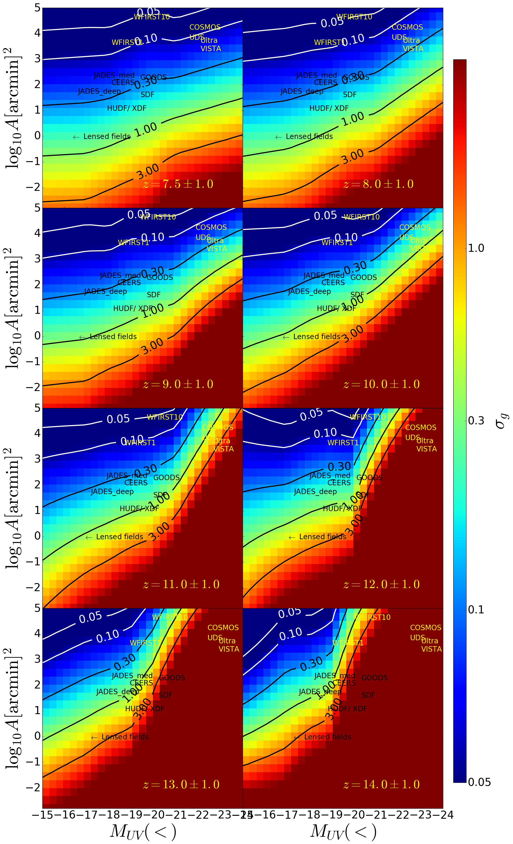
We use the results of the previous two sections to construct a cosmic variance calculator CV_AT_COSMIC_DAWN (all occurrences of ‘CV_AT_COSMIC_DAWN’ are hyperlinks to the github repository) for $z>7$ . In particular, CV_AT_COSMIC_DAWN uses the fitting results summarized in Table 1 and Eq. 5 to compute cosmic variances for $M_{UV}$ thresholds and redshifts listed in Table 1. For the redshifts and $M_{UV}$ thresholds which lie in between those listed in Table 1, we use linear interpolation to estimate the cosmic variance. Cosmic variance estimates made using CV_AT_COSMIC_DAWN are shown as dotted lines in Figure 4.

Survey	Instrument	Area	$H~(<)$	Reference
WFIRST10	WFIRST	$10~\mathrm{deg}^{2}$	$\sim 27.5$	WFIRST Science Sheet
WFIRST1	WFIRST	$1~\mathrm{deg}^{2}$	$\sim 28.5$	WFIRST Science Sheet
ultraVISTA	VISTA	$1~\mathrm{deg}^{2}$	$\sim 28.5$	McCracken, H. J. et al. 2012
JADES-medium	JWST	$\sim 190~\mathrm{arcmin}^{2}$	$\sim 29.7$	JADES survey overview
JADES-deep	JWST	$\sim 46~\mathrm{arcmin}^{2}$	$\sim 30.6$	JADES survey overviews
CEERS	JWST	$\sim 100~\mathrm{arcmin}^{2}$	$\sim 29$	Finkelstein et al. 2017
HUDF	HST	$\sim 10~\mathrm{arcmin}^{2}$	$\sim 27$	Rafelski et al. 2015
GOODS	HST	$\sim 160~\mathrm{arcmin}^{2}$	$\sim 27.7$	Grogin et al. 2011
COSMOS	HST	$\sim 2~\mathrm{deg}^{2}$	$\sim 25.5$	Grogin et al. 2011
UDS	HST	$\sim 0.8~\mathrm{deg}^{2}$	$\sim 25$	Grogin et al. 2011
SDF	HSC	$\sim 34.~\mathrm{arcmin}^{2}$	$\sim 27.5$	Kashikawa et al. 2004

Table 3: List of upcoming and current high redshift surveys using WFIRST, JWST, Hubble space telescope (HST), Hyper Suprime Cam (HSC) and Cosmic Assembly Near infrared Extra-gaLactic Survey (CANDELS). HUDF refers to Hubble Ultra Deep Field and SDF refers to Subaru Deep Field.

H(<)

is the detection limit in the

H

band of WFIRST

We use CV_AT_COSMIC_DAWN to summarize our results as a 2D color plot (Figure 9) on the $A-M_{UV}(<)$ plane. We also present our estimates in terms of the apparent magnitude in Appendix A. The cosmic variance ranges from $\sigma_{g}\sim 0.01$ to $\sigma_{g}\sim 10$ and is represented by pixels colored as blue to red respectively. The solid black lines show contours representing $\sigma_{g}\sim 0.1,0.3,1,3,10$ . We show all the recent and upcoming surveys listed in Table 3 as various points on the plane positioned approximately by their survey area and depth.

3.5 Implications for galaxy luminosity functions: Contribution of cosmic variance to total uncertainty

Figure 10: Top Panels:

\Phi

is the rest frame UV luminosity function. Different colors represent galaxies within simulation sub-volumes corresponding to different survey areas with

\Delta z=1

. For each color, the shaded region corresponds to uncertainty due to cosmic variance. For each color, the dashed lines are upper and lower limits representing the total field to field variance (cosmic variance + Poisson variance). Bottom Panels:

\delta_{\sigma}

is the ratio between the cosmic variance and the total field to field variance. Open stars (Livermore et al. 2017), open squares (Ishigaki et al. 2018), open diamonds (Bouwens et al. 2015), open circles (Laporte et al. 2012), filled stars (Bouwens et al. 2015), filled diamonds (McLeod et al. 2016), filled squares (Oesch et al. 2018) are observational measurements from current deep and lensed fields.

We now study the impact of cosmic variance on the galaxy luminosity function. In figure 10, we compute the luminosity function and the associated cosmic variance and total=cosmic+Poisson variance for various survey areas. The open and black points show current observational constraints. The cosmic variance, shown by the shaded regions, reflects the trends seen in Figure 4, and is broadly consistent with uncertainties in observational measurements which typically include cosmic variance estimates.

The bottom panels show the fraction ( $\delta_{\sigma}$ ) of the total uncertainty that is contributed by cosmic variance. For fixed magnitude, we see that as survey area decreases, $\delta_{\sigma}$ decreases. Likewise, for fixed survey area, we see that as galaxies become brighter, $\delta_{\sigma}$ decreases. This is expected since number counts decrease with decreasing survey area and with increasing luminosity, which increases the contribution from Poisson variance. Furthermore, we see that $\delta_{\sigma}>50\%$ , implying that cosmic variance is the more dominant contribution to the overall uncertainty as compared to Poisson variance, the only exceptions being samples with very small ( $\lesssim 10$ ) number counts (as also seen in Figure 5).

4 Possible uncertainties in the cosmic variance estimates

Our cosmic variance estimates are subject to uncertainties, particularly because the estimates are based on a single hydrodynamic simulation run with a fixed cosmology and galaxy formation modeling. The cosmic variance estimates depend on cosmology due to its effect on the halo bias and matter clustering, as well as the comoving survey volume. For instance, between WMAP (Hinshaw et al. 2013) and PLANCK (Planck Collaboration et al. 2016) cosmologies, the comoving survey volume changes by $\sim 15~\%$ ; the matter clustering changes by $\sim 4-10~\%$ (depending on the length scale) and the halo bias (based on the Tinker et al. 2010 model) changes by $\sim 0.5-3~\%$ (depending on the halo mass scale). Adding these contributions up, we can overall expect a difference of $\sim 25-30~\%$ between cosmic variances $\sigma_{g}$ predicted by the WMAP and PLANCK cosmologies. Additionally, uncertainties in the galaxy formation physics can also affect our cosmic variance estimates. In particular, a given sample of galaxies can populate haloes of different masses in different recipes of galaxy formation, thereby affecting the clustering amplitudes. For example, if the star formation within a galaxy sample is extremely ‘bursty’ or ‘episodic’, they may reside within a relatively small fraction of lower mass (more abundant) haloes, compared to a model that does not lead to bursty star formation. This will lead to lower clustering amplitude (for a fixed number density or luminosity function). Finally, we make several approximations in computing the cosmic variance: we use cuboidal volumes through the box with fixed transverse extent, rather than lightcones, and do not include the time evolution across the redshift interval. We expect that the errors due to these approximations will not significantly affect our predictions.

5 Summary and Conclusions

In this work, we used the recent BlueTides simulation to estimate the cosmic variance for $z>7$ galaxies to be detected by the planned deep surveys of JWST and WFIRST. Cosmic variance is expected to be a significant, potentially dominant source of uncertainty given the exceptionally strong clustering power (galaxy bias $\gtrsim 6$ ) of these galaxies seen in recent observations. We express the cosmic variance as an integral of the two-point correlation function over the survey volume, as commonly done in the literature (Peebles 1980; Moster et al. 2011).

The resolution and volume enables BlueTides to probe the large scale bias, and therefore the cosmic variance of $z>7$ galaxies with $M_{UV}\sim-16$ to $M_{UV}\sim-22$ over survey areas $\sim 0.1~\mathrm{arcmin}^{2}$ to $\sim 10~\mathrm{deg}^{2}$ . Within this regime, the cosmic variance has a power law dependence on survey volume (with exponent $\sim-0.25$ to $-0.45$ ). More luminous galaxies have larger cosmic variance than faint galaxies.

The above trends can be put in the context of upcoming deep surveys. The largest planned deep survey will naturally suffer from the least amount of cosmic variance; this corresponds to the $10~\mathrm{deg}^{2}$ field of WFIRST, which will have a cosmic variance ranging from $\sim 3-10\%$ , except for $M_{UV}<-22$ galaxies at $z>12$ where the cosmic variance can exceed $\sim 10\%$ . Upcoming JWST medium/ deep surveys (up to areas of $100~\mathrm{arcmin}^{2}$ ) will have a cosmic variance of about $20-50\%$ for $M_{UV}$ between $-16$ to $-20$ . At the other end, the smallest surveys are the lensed surveys (Hubble Frontier fields) and are most susceptible to cosmic variance. They have cosmic variance $\gtrsim 40\%$ over the entire range of magnitudes and redshifts. These are the only existing surveys that can probe the faint ( $M_{UV}$ thresholds between $\sim-13$ to $-16$ ) end of the luminosity function. In order for these measurements to provide useful constraints (e.g. on the nature of dark matter), the cosmic variance must be contained within $100\%$ . For $M_{UV}$ thresholds up to $-16$ , the cosmic variance is within $100\%$ for $z\sim 7-11$ for the entire range of effective volumes between $\sim 6-14~(\mathrm{Mpc}/h)^{3}$ . At higher redshifts, effective volumes of $\gtrsim 8~(\mathrm{Mpc}/h)^{3}$ and $\gtrsim 12~(\mathrm{Mpc}/h)^{3}$ at $z\sim 12$ and $z\sim 14$ respectively, to keep the cosmic variance within $100\%$ .

Lastly, we study the impact of cosmic variance on the luminosity function and estimate the contribution of cosmic variance to the total uncertainty. We find that across all redshifts and magnitude bins (with the exception of the most luminous bins with number counts $\lesssim 10$ objects), cosmic variance is the more dominant component of the uncertainty, as compared to Poisson variance.

We capture our results in the form of simple fitting functions and encode them in an online cosmic variance calculator (CV_AT_COSMIC_DAWN) which we publicly release.

Appendix A Presenting cosmic variance in terms of telescope survey parameters

In addition to presenting cosmic variance as a function of the rest frame intrinsic UV magnitude, it is also useful (for observers in particular) to present our estimates directly in terms of the apparent magnitude, which is fixed for a given survey. We therefore, in Figure 11, also present our estimates in terms of the apparent magnitude. We choose the $H$ band magnitude of WFIRST, and present our estimates up to redshift 10.

Acknowledgements

We acknowledge funding from NSF ACI-1614853, NSF AST1517593, NSF AST-1616168, NSF AST-1716131, NASA ATP NNX17AK56G and NASA ATP 17-0123, and the BLUEWATERS PAID program. NSF:- National Science Foundation, ACI:- Division of Advanced Cyber Infrastructure, AST:- Division of Astronomical Sciences, NASA:- National Aeronautics and Space Administration, ATP:- Astrophysics Theory Program. The BlueTides simulation was run on the BLUEWATERS facility at the National Center for Supercomputing Applications.

References

Artale et al. (2017) Artale M. C., et al., 2017, MNRAS, 470, 1771
Bañados et al. (2018) Bañados E., et al., 2018, Nature, 553, 473
Barone-Nugent et al. (2014) Barone-Nugent R. L., et al., 2014, ApJ, 793, 17
Battaglia et al. (2013) Battaglia N., Trac H., Cen R., Loeb A., 2013, ApJ, 776, 81
Behroozi et al. (2013) Behroozi P. S., Wechsler R. H., Wu H.-Y., 2013, ApJ, 762, 109
Bhowmick et al. (2018a) Bhowmick A. K., Di Matteo T., Feng Y., Lanusse F., 2018a, MNRAS, 474, 5393
Bhowmick et al. (2018b) Bhowmick A. K., Campbell D., Di Matteo T., Feng Y., 2018b, MNRAS, 480, 3177
Blaizot et al. (2006) Blaizot J., et al., 2006, MNRAS, 369, 1009
Bouwens et al. (2015) Bouwens R. J., et al., 2015, ApJ, 803, 34
Bouwens et al. (2017) Bouwens R. J., Oesch P. A., Illingworth G. D., Ellis R. S., Stefanon M., 2017, ApJ, 843, 129
Bradač et al. (2009) Bradač M., et al., 2009, The Astrophysical Journal, 706, 1201
Campbell et al. (2018) Campbell D., van den Bosch F. C., Padmanabhan N., Mao Y.-Y., Zentner A. R., Lange J. U., Jiang F., Villarreal A., 2018, MNRAS, 477, 359
Chabrier (2003) Chabrier G., 2003, PASP, 115, 763
Chen et al. (2019) Chen Y., Mo H. J., Li C., Wang H., Yang X., Zhou S., Zhang Y., 2019, ApJ, 872, 180
Davis et al. (1985) Davis M., Efstathiou G., Frenk C. S., White S. D. M., 1985, ApJ, 292, 371
Di Matteo et al. (2005) Di Matteo T., Springel V., Hernquist L., 2005, Nature, 433, 604
Di Matteo et al. (2017) Di Matteo T., Croft R. A. C., Feng Y., Waters D., Wilkins S., 2017, MNRAS, 467, 4243
Duncan et al. (2014) Duncan K., et al., 2014, MNRAS, 444, 2960
Feng et al. (2015) Feng Y., Di Matteo T., Croft R., Tenneti A., Bird S., Battaglia N., Wilkins S., 2015, ApJ, 808, L17
Feng et al. (2016) Feng Y., Di-Matteo T., Croft R. A., Bird S., Battaglia N., Wilkins S., 2016, MNRAS, 455, 2778
Finkelstein et al. (2017) Finkelstein S., et al., 2017, The Cosmic Evolution Early Release Science (CEERS) Survey, JWST Proposal ID 1345. Cycle 0 Early Release Science
Fioc & Rocca-Volmerange (1997) Fioc M., Rocca-Volmerange B., 1997, A&A, 326, 950
Gardner et al. (2006) Gardner J. P., et al., 2006, Space Sci. Rev., 123, 485
Grogin et al. (2011) Grogin N. A., et al., 2011, ApJS, 197, 35
Harikane et al. (2016) Harikane Y., et al., 2016, ApJ, 821, 123
Hinshaw et al. (2013) Hinshaw G., et al., 2013, ApJS, 208, 19
Ishigaki et al. (2018) Ishigaki M., Kawamata R., Ouchi M., Oguri M., Shimasaku K., Ono Y., 2018, ApJ, 854, 73
Jauzac et al. (2015) Jauzac M., et al., 2015, MNRAS, 452, 1437
Kashikawa et al. (2004) Kashikawa N., et al., 2004, PASJ, 56, 1011
Katz et al. (1996) Katz N., Weinberg D. H., Hernquist L., 1996, ApJS, 105, 19
Kawamata et al. (2016) Kawamata R., Oguri M., Ishigaki M., Shimasaku K., Ouchi M., 2016, ApJ, 819, 114
Khandai et al. (2015) Khandai N., Di Matteo T., Croft R., Wilkins S., Feng Y., Tucker E., DeGraf C., Liu M.-S., 2015, MNRAS, 450, 1349
Koekemoer et al. (2017) Koekemoer A. M., et al., 2017, in American Astronomical Society Meeting Abstracts #230. p. 316.13
Krumholz & Gnedin (2011) Krumholz M. R., Gnedin N. Y., 2011, ApJ, 729, 36
Laporte et al. (2012) Laporte N., et al., 2012, A&A, 542, L31
Livermore et al. (2017) Livermore R. C., Finkelstein S. L., Lotz J. M., 2017, ApJ, 835, 113
McCracken, H. J. et al. (2012) McCracken, H. J. et al., 2012, A&A, 544, A156
McLeod et al. (2016) McLeod D. J., McLure R. J., Dunlop J. S., 2016, MNRAS, 459, 3812
Menci et al. (2016) Menci N., Sanchez N. G., Castellano M., Grazian A., 2016, ApJ, 818, 90
Menci et al. (2017) Menci N., Merle A., Totzauer M., Schneider A., Grazian A., Castellano M., Sanchez N. G., 2017, ApJ, 836, 61
Moster et al. (2010) Moster B. P., Somerville R. S., Maulbetsch C., van den Bosch F. C., Macciò A. V., Naab T., Oser L., 2010, ApJ, 710, 903
Moster et al. (2011) Moster B. P., Somerville R. S., Newman J. A., Rix H.-W., 2011, ApJ, 731, 113
Nelson et al. (2015) Nelson D., et al., 2015, Astronomy and Computing, 13, 12
Ni et al. (2018) Ni Y., Di Matteo T., Feng Y., Croft R. A. C., Tenneti A., 2018, MNRAS, 481, 4877
Ni et al. (2019) Ni Y., Wang M.-Y., Feng Y., Di Matteo T., 2019, arXiv e-prints, p. arXiv:1904.01604
Oesch et al. (2016) Oesch P. A., et al., 2016, ApJ, 819, 129
Oesch et al. (2018) Oesch P. A., et al., 2018, ApJS, 237, 12
Park et al. (2017) Park J., et al., 2017, MNRAS, 472, 1995
Peebles (1980) Peebles P. J. E., 1980, The large-scale structure of the universe
Planck Collaboration et al. (2016) Planck Collaboration et al., 2016, A&A, 594, A13
Rafelski et al. (2015) Rafelski M., et al., 2015, AJ, 150, 31
Schaye et al. (2015) Schaye J., et al., 2015, MNRAS, 446, 521
Somerville & Davé (2015) Somerville R. S., Davé R., 2015, ARA&A, 53, 51
Somerville et al. (2004) Somerville R. S., Lee K., Ferguson H. C., Gardner J. P., Moustakas L. A., Giavalisco M., 2004, ApJ, 600, L171
Somerville et al. (2008) Somerville R. S., Hopkins P. F., Cox T. J., Robertson B. E., Hernquist L., 2008, MNRAS, 391, 481
Song et al. (2016) Song M., et al., 2016, ApJ, 825, 5
Spergel et al. (2015) Spergel D., et al., 2015, arXiv e-prints, p. arXiv:1503.03757
Springel & Hernquist (2003) Springel V., Hernquist L., 2003, MNRAS, 339, 289
Springel et al. (2005) Springel V., Di Matteo T., Hernquist L., 2005, MNRAS, 361, 776
Tenneti et al. (2017) Tenneti A., Di Matteo T., Croft R., Garcia T., Feng Y., 2017, preprint, (arXiv:1708.03373)
Tenneti et al. (2019) Tenneti A., Wilkins S. M., Di Matteo T., Croft R. A. C., Feng Y., 2019, MNRAS, 483, 1388
Tinker et al. (2010) Tinker J. L., Robertson B. E., Kravtsov A. V., Klypin A., Warren M. S., Yepes G., Gottlöber S., 2010, ApJ, 724, 878
Trenti & Stiavelli (2008) Trenti M., Stiavelli M., 2008, ApJ, 676, 767
Ucci et al. (2020) Ucci G., et al., 2020, arXiv e-prints, p. arXiv:2004.11096
Vogelsberger et al. (2013) Vogelsberger M., Genel S., Sijacki D., Torrey P., Springel V., Hernquist L., 2013, MNRAS, 436, 3031
Vogelsberger et al. (2014) Vogelsberger M., et al., 2014, MNRAS, 444, 1518
Waters et al. (2016a) Waters D., Wilkins S. M., Di Matteo T., Feng Y., Croft R., Nagai D., 2016a, MNRAS, 461, L51
Waters et al. (2016b) Waters D., Di Matteo T., Feng Y., Wilkins S. M., Croft R. A. C., 2016b, MNRAS, 463, 3520
Wilkins et al. (2016a) Wilkins S. M., Feng Y., Di-Matteo T., Croft R., Stanway E. R., Bouwens R. J., Thomas P., 2016a, MNRAS, 458, L6
Wilkins et al. (2016b) Wilkins S. M., Feng Y., Di-Matteo T., Croft R., Stanway E. R., Bunker A., Waters D., Lovell C., 2016b, MNRAS, 460, 3170
Wilkins et al. (2018) Wilkins S. M., Feng Y., Di Matteo T., Croft R., Lovell C. C., Thomas P., 2018, MNRAS, 473, 5363
Yang et al. (2012) Yang X., Mo H. J., van den Bosch F. C., Zhang Y., Han J., 2012, ApJ, 752, 41
Yung et al. (2019a) Yung L. Y. A., Somerville R. S., Popping G., Finkelstein S. L., Ferguson H. C., Davé R., 2019a, arXiv e-prints, p. arXiv:1901.05964
Yung et al. (2019b) Yung L. Y. A., Somerville R. S., Finkelstein S. L., Popping G., Davé R., 2019b, MNRAS, 483, 2983

Cosmic variance of z>7z>7 galaxies: Prediction from BlueTides