跳到论文正文
W Papers独立论文阅读器 arXiv:1908.02694 论文正文 计算阅读时间 · 0%
引用这篇论文根据当前论文元数据生成,正式投稿前建议核对。


License: arXiv.org perpetual non-exclusive license
arXiv:1908.02694v2 [physics.comp-ph] 08 Aug 2019

∎

A distributed active subspace method for scalable surrogate modeling of function valued outputs

Hayley Guy Affiliation: Department of Mathematics, North Carolina State University E-mail: hguy@ncsu.edu    Alen Alexanderian Affiliation: Department of Mathematics, North Carolina State University E-mail: alexanderian@ncsu.edu    Meilin Yu Affiliation: Department of Mechanical Engineering, The University of Maryland, Baltimore County E-mail: mlyu@umbc.edu
Abstract

We present a distributed active subspace method for training surrogate models of complex physical processes with high-dimensional inputs and function valued outputs. Specifically, we represent the model output with a truncated Karhunen–Loève (KL) expansion, screen the structure of the input space with respect to each KL mode via the active subspace method, and finally form an overall surrogate model of the output by combining surrogates of individual output KL modes. To ensure scalable computation of the gradients of the output KL modes, needed in active subspace discovery, we rely on adjoint-based gradient computation. The proposed method combines benefits of active subspace methods for input dimension reduction and KL expansions used for spectral representation of the output field. We provide a mathematical framework for the proposed method and conduct an error analysis of the mixed KL active subspace approach. Specifically, we provide an error estimate that quantifies errors due to active subspace projection and truncated KL expansion of the output. We demonstrate the numerical performance of the surrogate modeling approach with an application example from biotransport.

Keywords

Distributed active subspace; Karhunen–Loève expansion; Dimension reduction; Function valued outputs; Porous medium flow; Biotransport.

1 Introduction

Models with uncertain input parameters are common in modeling of complex systems. Computational studies such as forward uncertainty propagation, optimization, or parameter estimation require repeated evaluation of the model. These tasks become challenging for expensive-to-evaluate complex models. To address this challenge, surrogate models are often used. By approximating the mapping from the uncertain input parameters to output quantities of interest (QoIs), using a surrogate model, one can replace expensive model evaluations by inexpensive surrogate model evaluations. Examples of surrogate modeling tools include polynomial chaos expansion GhanemSpanos90; LeMaitreKnio10, multivariate adaptive regression splines friedman93, and Gaussian processes RasmussenWilliams06.

In the present work, we consider surrogate construction for models of the form

y=f⁡(𝒙,𝝃),y=f({\mathchoice{\mbox{\boldmath$\displaystyle{x}$}}{\mbox{\boldmath$\textstyle{x}$}}{\mbox{\boldmath$\scriptstyle{x}$}}{\mbox{\boldmath$\scriptscriptstyle{x}$}}},{\mathchoice{\mbox{\boldmath$\displaystyle{\xi}$}}{\mbox{\boldmath$\textstyle{\xi}$}}{\mbox{\boldmath$\scriptstyle{\xi}$}}{\mbox{\boldmath$\scriptscriptstyle{\xi}$}}}), (1)

where 𝒙\textstyle{x} belongs to a spatial domain and 𝝃∈ℝNp{\mathchoice{\mbox{\boldmath$\displaystyle{\xi}$}}{\mbox{\boldmath$\textstyle{\xi}$}}{\mbox{\boldmath$\scriptstyle{\xi}$}}{\mbox{\boldmath$\scriptscriptstyle{\xi}$}}}\in\mathbb{R}^{N_{p}} is a vector of uncertain parameters. In our target applications ff is defined in terms of the solution of a partial differential equation (PDE) that is parameterized by a high-dimensional input parameter. Albeit, the proposed framework can be adapted to more general settings.

A simple approach is to construct a surrogate model pointwise in 𝒙\textstyle{x}. Specifically, discretizing the spatial domain by grid points {𝒙i}i=1Nx\{{\mathchoice{\mbox{\boldmath$\displaystyle{x}$}}{\mbox{\boldmath$\textstyle{x}$}}{\mbox{\boldmath$\scriptstyle{x}$}}{\mbox{\boldmath$\scriptscriptstyle{x}$}}}_{i}\}_{i=1}^{N_{x}}, we may consider approximating f⁡(𝒙i,𝝃)f({\mathchoice{\mbox{\boldmath$\displaystyle{x}$}}{\mbox{\boldmath$\textstyle{x}$}}{\mbox{\boldmath$\scriptstyle{x}$}}{\mbox{\boldmath$\scriptscriptstyle{x}$}}}_{i},{\mathchoice{\mbox{\boldmath$\displaystyle{\xi}$}}{\mbox{\boldmath$\textstyle{\xi}$}}{\mbox{\boldmath$\scriptstyle{\xi}$}}{\mbox{\boldmath$\scriptscriptstyle{\xi}$}}}), by constructing surrogate models f^i​(𝝃)≈f⁡(𝒙i,⋅)\hat{f}_{i}({\mathchoice{\mbox{\boldmath$\displaystyle{\xi}$}}{\mbox{\boldmath$\textstyle{\xi}$}}{\mbox{\boldmath$\scriptstyle{\xi}$}}{\mbox{\boldmath$\scriptscriptstyle{\xi}$}}})\approx f({\mathchoice{\mbox{\boldmath$\displaystyle{x}$}}{\mbox{\boldmath$\textstyle{x}$}}{\mbox{\boldmath$\scriptstyle{x}$}}{\mbox{\boldmath$\scriptscriptstyle{x}$}}}_{i},\cdot), i=1,…,Nxi=1,\ldots,N_{x}. This straightforward approach can be useful in some cases, however, the power of many of the surrogate modeling approaches can be fully realized if one optimizes them for each 𝒙i{\mathchoice{\mbox{\boldmath$\displaystyle{x}$}}{\mbox{\boldmath$\textstyle{x}$}}{\mbox{\boldmath$\scriptstyle{x}$}}{\mbox{\boldmath$\scriptscriptstyle{x}$}}}_{i} in the computational grid. This is a computationally expensive task and might become prohibitive if the parameter dimension Np{N_{p}} is large (e.g., Np≥100{N_{p}}\geq 100), the model exhibits large variations in its response to parametric uncertainties over the spatial domain, or the grid point number NxN_{x} is large, as can happen in two or three-dimensional geometries.

We seek an efficient surrogate modeling approach, for models of the form (1), whose complexity in terms of the number of model evaluations does not scale with the dimension Np{N_{p}} of the input parameters. To enable this, we need a method that is structure exploiting. In particular, we seek to discover and utilize informative low-dimensional subspaces in the input space and low-dimensional spectral representations of the model output. The former uses ideas from active subspace methods Constantine15 and the latter uses Karhunen–Loève (KL) expansions Loeve77; GhanemSpanos90. This proposed approach decouples the spatial (i.e. 𝒙\textstyle{x}) dimensions and those of the random variable 𝝃\textstyle{\xi} and exposes important structures that can be used for building efficient surrogate models.

Related work. KL expansions have been used in many works for representing random field parameters in physics models; see e.g., Ghanem98; LeMaitreReaganNajmEtAl02; XiuKarniadakis03; LeMaitreKnio04; BabuvskaNobileTempone07; Doostan07; SaadGhanem09; MatthiesKeese05; Graham15KuoKuoNicholsEtAl15; Elman17. KL expansions can also be used to represent random field outputs of physics models, as done in the present work. In models governed by PDEs the output field often exhibits favorable regularity properties and can be represented by a KL expansion with a relatively small number of KL terms. Examples of this appear for instance in our recent works CleavesAlexanderianGuyEtAl19; ARSY2019 for models governed by elliptic PDEs.

The active subspace method Russi10; constantine2014; Constantine15 has become a popular approach in recent years for input parameter dimension reduction and surrogate modeling. This method seeks to identify important linear combinations of the input parameters. A brief summary of the active subspace method, for approximating scalar valued models, has been provided in Section 2. The active subspace method has been successfully used for uncertainty analysis in models with scalar valued responses, in a host of engineering applications; examples include scramjet analysis Scramjet15, wing shape optimization ShapeOpt14, hydrologic modeling ConstantineGeo15, battery modeling ConstantineBattery17, and kinetic model uncertainty analysis ji2018shared. Recently, there have been efforts in extending the active subspace method to vector valued functions. In zahm2018gradient the authors find an upper bound for the error of a ridge function approximation of the original (vector valued) function, and construct an approximating function by minimzing that upper bound. In ji2018shared an interesting approach is introduced for simultaneously approximating multiple outputs using a single low-dimensional shared subspace. The shared subspace is identified by solving a least-squares system to compute an appropriate combination of single-output active subspaces.

We also mention another related and popular class of methods for parameter dimension reduction: variance based Sobol:1990; Sobol:2001 and derivative based SobolKucherenko09; KucherenkoIooss17 global sensitivity analysis (GSA). These methods provide means of identifying unimportant model inputs, hence reducing the dimension of the input parameter vector. Derivative based methods are especially attractive, as they can be used to efficiently screen for unimportant input parameters, after which a surrogate model can be computed as a function of a reduced set of parameters. While GSA approaches have traditionally been applied to models with scalar outputs, extensions of GSA methods to vectorial and function valued outputs appear in several recent works GamboaJanonKleinEtAl14; AlexanderianGremaudSmith17; CleavesAlexanderianGuyEtAl19.

In practice, the active subspace method tends to be very effective in reducing the input dimension as important directions in the input parameter space are identified. This is, in contrast to seeking reduced parameter subsets, as identified by GSA approaches. We note however that utility of GSA goes beyond input parameter dimension reduction—GSA provides valuable insight regarding a model by identifying key contributors to model variability. Also, we mention an interesting link between derivative based GSA and active subspaces through the idea of activity scores as detailed in ConstantineDiaz17; computing active subspaces provides, as a byproduct, approximations to derivative based global sensitivity measures, for scalar valued models.

Our approach and contributions. In our proposed approach, we combine active subspaces and KL expansions to enable efficient surrogate modeling for function valued QoIs. Specifically, we consider a suitably truncated KL decomposition

f⁡(𝒙,𝝃)≈f¯​(𝒙)+∑k=1Nλk​fk​(𝝃)​ϕk​(𝒙),\begin{array}[]{cc}f({\mathchoice{\mbox{\boldmath$\displaystyle{x}$}}{\mbox{\boldmath$\textstyle{x}$}}{\mbox{\boldmath$\scriptstyle{x}$}}{\mbox{\boldmath$\scriptscriptstyle{x}$}}},{\mathchoice{\mbox{\boldmath$\displaystyle{\xi}$}}{\mbox{\boldmath$\textstyle{\xi}$}}{\mbox{\boldmath$\scriptstyle{\xi}$}}{\mbox{\boldmath$\scriptscriptstyle{\xi}$}}})\approx\bar{f}({\mathchoice{\mbox{\boldmath$\displaystyle{x}$}}{\mbox{\boldmath$\textstyle{x}$}}{\mbox{\boldmath$\scriptstyle{x}$}}{\mbox{\boldmath$\scriptscriptstyle{x}$}}})+\sum\limits_{k=1}^{N}\sqrt{\lambda_{k}}f_{k}({\mathchoice{\mbox{\boldmath$\displaystyle{\xi}$}}{\mbox{\boldmath$\textstyle{\xi}$}}{\mbox{\boldmath$\scriptstyle{\xi}$}}{\mbox{\boldmath$\scriptscriptstyle{\xi}$}}})\phi_{k}({\mathchoice{\mbox{\boldmath$\displaystyle{x}$}}{\mbox{\boldmath$\textstyle{x}$}}{\mbox{\boldmath$\scriptstyle{x}$}}{\mbox{\boldmath$\scriptscriptstyle{x}$}}}),\\ \end{array}

where f¯\bar{f} is the mean of the process f⁡(𝒙,𝝃)f({\mathchoice{\mbox{\boldmath$\displaystyle{x}$}}{\mbox{\boldmath$\textstyle{x}$}}{\mbox{\boldmath$\scriptstyle{x}$}}{\mbox{\boldmath$\scriptscriptstyle{x}$}}},{\mathchoice{\mbox{\boldmath$\displaystyle{\xi}$}}{\mbox{\boldmath$\textstyle{\xi}$}}{\mbox{\boldmath$\scriptstyle{\xi}$}}{\mbox{\boldmath$\scriptscriptstyle{\xi}$}}}) and (λk,ϕk)(\lambda_{k},\phi_{k}) are the eigenpairs of the covariance operator of the process. This way, the model uncertainty is encoded in the KL modes, fkf_{k}, k=1,…,Nk=1,\ldots,N. In many cases a small NN can be very effective in approximating ff. These KL modes can then be approximated efficiently using the active subspace approach. The active subspace approach requires the gradients of fkf_{k}, which are scalar functions of the random vector 𝝃\textstyle{\xi}. For such functions, adjoint state approaches provide efficient means of computing the required gradients. Specifically, gradients can be computed as a cost, in terms of model evaluations, that does not scale with the dimension of the input parameter 𝝃\textstyle{\xi}. Realizing the proposed approach requires (i) a rigorous functional framework upon which efficient computational algorithms can be built; and (ii) a systematic computational procedure that guides efficient implementations. These have been detailed in Section 3.

We deploy our proposed framework in the context of flows in biological tissues. Specifically, in Section 4, we tackle biotransport in porous tumors with high-dimensional random inputs (i.e., the permeability field) and random field outputs (i.e., the pressure distribution in tumors). Biological tissues usually have highly heterogeneous, even uncertain, material properties Frontier:16. The biotransport process such as drug delivery in tissues thus can exhibit “unpredictable” behaviors due to the uncertainties in tissue material properties Deb:09CPD. Since the unpredictability can adversely affect the effectiveness of therapy, quantifying variability in biotransport due to uncertain material properties has a high impact on clinical trial protocol design. However, conducting useful uncertainty quantification studies on biotransport is challenging due to the high dimension of the input parameter space, e.g. permeability and porosity AlexanderianZhuSalloumEtAl17. We find that efficient-to-evaluate and accurate surrogate models can be computed at a modest computational cost, with our proposed framework. The presented computational experiments also indicate that the present method can be used successfully in more general porous medium flow problems, where Darcy flow is a reasonable model. Further investigations of the proposed surrogate modeling method in more complex flow models is subject of our future work.

The contributions of this article are summarized as follows:

  • ∘\circ

    We present a mathematical framework and computational method for surrogate modeling for models with high-dimensional inputs and function valued outputs that uses KL expansions for output dimension reduction, active subspaces for input dimension reduction, and adjoint based gradient computation as needed in the active subspace method.

  • ∘\circ

    We analyze the errors due to active subspace projection and output KL truncation. The presented analysis provides insight on the interplay between these two important sources of errors.

  • ∘\circ

    We present comprehensive computational results in the context of a biotransport application problem that test various aspects of the proposed surrogate modeling method. We mention that the computational studies, to our knowledge, are the first of a kind in the area of biotransport modeling in tissues with uncertain heterogeneous material properties.

2 Background on active subspace

One common approach to input dimension reduction is to identify a subset of input model parameters that are the most important to model variability. This is done typically using a local or global sensitivity analysis approach KucherenkoIooss17; IoossSaltelli17; PrieurTarantola17. The active subspace approach is different; it identifies a set of important directions in the input parameter space rather than giving importance to one input over another. We can rotate the coordinates to align with the directions of strongest variation. Each direction can be considered as a set of weights that define a linear combination of all of the inputs. Directions where the inputs do not vary much are ignored.

Consider a model

y=g⁡(𝝃),𝝃∈ℝNp.y=g({\mathchoice{\mbox{\boldmath$\displaystyle{\xi}$}}{\mbox{\boldmath$\textstyle{\xi}$}}{\mbox{\boldmath$\scriptstyle{\xi}$}}{\mbox{\boldmath$\scriptscriptstyle{\xi}$}}}),\quad{\mathchoice{\mbox{\boldmath$\displaystyle{\xi}$}}{\mbox{\boldmath$\textstyle{\xi}$}}{\mbox{\boldmath$\scriptstyle{\xi}$}}{\mbox{\boldmath$\scriptscriptstyle{\xi}$}}}\in\mathbb{R}^{N_{p}}.

We assume the uncertain parameters 𝝃\textstyle{\xi} have an associated probability density function π⁡(𝝃)\pi({\mathchoice{\mbox{\boldmath$\displaystyle{\xi}$}}{\mbox{\boldmath$\textstyle{\xi}$}}{\mbox{\boldmath$\scriptstyle{\xi}$}}{\mbox{\boldmath$\scriptscriptstyle{\xi}$}}}) that is supported on Ω⊆ℝNp\Omega\subseteq\mathbb{R}^{N_{p}}. Assume gg is square integrable and has continuous partial derivatives with respect to 𝝃\textstyle{\xi}. The following matrix plays a key role in active subspace construction:

𝐒=∫Ω∇g(𝝃)∇g(𝝃)Tπ(𝝃)d𝝃,\mathbf{{S}}=\int_{\Omega}\nabla g({\mathchoice{\mbox{\boldmath$\displaystyle{\xi}$}}{\mbox{\boldmath$\textstyle{\xi}$}}{\mbox{\boldmath$\scriptstyle{\xi}$}}{\mbox{\boldmath$\scriptscriptstyle{\xi}$}}})\,\nabla g({\mathchoice{\mbox{\boldmath$\displaystyle{\xi}$}}{\mbox{\boldmath$\textstyle{\xi}$}}{\mbox{\boldmath$\scriptstyle{\xi}$}}{\mbox{\boldmath$\scriptscriptstyle{\xi}$}}})^{T}\pi({\mathchoice{\mbox{\boldmath$\displaystyle{\xi}$}}{\mbox{\boldmath$\textstyle{\xi}$}}{\mbox{\boldmath$\scriptstyle{\xi}$}}{\mbox{\boldmath$\scriptscriptstyle{\xi}$}}})d{\mathchoice{\mbox{\boldmath$\displaystyle{\xi}$}}{\mbox{\boldmath$\textstyle{\xi}$}}{\mbox{\boldmath$\scriptstyle{\xi}$}}{\mbox{\boldmath$\scriptscriptstyle{\xi}$}}}, (2)

where ∇g\nabla g is the gradient of gg. The matrix 𝐒\mathbf{{S}} is symmetric and positive semi-definite with spectral decomposition

𝐒=𝐖​𝚲​𝐖T,𝚲=diag​(λ1,⋯,λNp).\mathbf{{S}}=\mathbf{{W}}\mathbf{{\Lambda}}\mathbf{{W}}^{T},\quad\mathbf{{\Lambda}}=\text{diag}(\lambda_{1},\cdots,\lambda_{N_{p}}).

The eigenvalues λi\lambda_{i}’s are sorted in descending order λ1≥⋯≥λNp≥0\lambda_{1}\geq\cdots\geq\lambda_{N_{p}}\geq 0 and 𝐖\mathbf{{W}} contains the orthonormal eigenvectors of 𝐒\mathbf{{S}}.

The active subspace is determined by the dominant eigenvectors of 𝐒\mathbf{{S}}. Specifically, we partition the eigenvalues and eigenvectors according to

𝚲=[𝚲1𝚲2],𝐖=[𝐖1𝐖2],\mathbf{{\Lambda}}=\begin{bmatrix}\mathbf{{\Lambda}}_{1}&\\ &\mathbf{{\Lambda}}_{2}\end{bmatrix},\quad\mathbf{{W}}=\begin{bmatrix}\mathbf{{W}}_{1}&\mathbf{{W}}_{2}\end{bmatrix}, (3)

where 𝚲1∈ℝr×r\mathbf{{\Lambda}}_{1}\in\mathbb{R}^{r\times r} is a diagonal matrix with the dominant eigenvalues on its diagonal; and 𝐖1\mathbf{{W}}_{1} contains the corresponding eigenvectors 𝒘1,…​𝒘r{\mathchoice{\mbox{\boldmath$\displaystyle{w}$}}{\mbox{\boldmath$\textstyle{w}$}}{\mbox{\boldmath$\scriptstyle{w}$}}{\mbox{\boldmath$\scriptscriptstyle{w}$}}}_{1},\ldots{\mathchoice{\mbox{\boldmath$\displaystyle{w}$}}{\mbox{\boldmath$\textstyle{w}$}}{\mbox{\boldmath$\scriptstyle{w}$}}{\mbox{\boldmath$\scriptscriptstyle{w}$}}}_{r} as its columns. These columns span the dominant eigenspace of 𝐒\mathbf{{S}}—the active subspace.

Given 𝝃\textstyle{\xi} we define 𝒚=𝐖1T​𝝃∈ℝr{\mathchoice{\mbox{\boldmath$\displaystyle{y}$}}{\mbox{\boldmath$\textstyle{y}$}}{\mbox{\boldmath$\scriptstyle{y}$}}{\mbox{\boldmath$\scriptscriptstyle{y}$}}}=\mathbf{{W}}_{1}^{T}{\mathchoice{\mbox{\boldmath$\displaystyle{\xi}$}}{\mbox{\boldmath$\textstyle{\xi}$}}{\mbox{\boldmath$\scriptstyle{\xi}$}}{\mbox{\boldmath$\scriptscriptstyle{\xi}$}}}\in\mathbb{R}^{r} and 𝒛=𝐖2T​𝝃∈ℝNp−r{\mathchoice{\mbox{\boldmath$\displaystyle{z}$}}{\mbox{\boldmath$\textstyle{z}$}}{\mbox{\boldmath$\scriptstyle{z}$}}{\mbox{\boldmath$\scriptscriptstyle{z}$}}}=\mathbf{{W}}_{2}^{T}{\mathchoice{\mbox{\boldmath$\displaystyle{\xi}$}}{\mbox{\boldmath$\textstyle{\xi}$}}{\mbox{\boldmath$\scriptstyle{\xi}$}}{\mbox{\boldmath$\scriptscriptstyle{\xi}$}}}\in\mathbb{R}^{{N_{p}}-r}, and note that

𝝃=𝐖1​𝐖1T​𝝃+𝐖2​𝐖2T​𝝃=𝐖1​𝒚+𝐖2​𝒛.{\mathchoice{\mbox{\boldmath$\displaystyle{\xi}$}}{\mbox{\boldmath$\textstyle{\xi}$}}{\mbox{\boldmath$\scriptstyle{\xi}$}}{\mbox{\boldmath$\scriptscriptstyle{\xi}$}}}=\mathbf{{W}}_{1}\mathbf{{W}}_{1}^{T}{\mathchoice{\mbox{\boldmath$\displaystyle{\xi}$}}{\mbox{\boldmath$\textstyle{\xi}$}}{\mbox{\boldmath$\scriptstyle{\xi}$}}{\mbox{\boldmath$\scriptscriptstyle{\xi}$}}}+\mathbf{{W}}_{2}\mathbf{{W}}_{2}^{T}{\mathchoice{\mbox{\boldmath$\displaystyle{\xi}$}}{\mbox{\boldmath$\textstyle{\xi}$}}{\mbox{\boldmath$\scriptstyle{\xi}$}}{\mbox{\boldmath$\scriptscriptstyle{\xi}$}}}=\mathbf{{W}}_{1}{\mathchoice{\mbox{\boldmath$\displaystyle{y}$}}{\mbox{\boldmath$\textstyle{y}$}}{\mbox{\boldmath$\scriptstyle{y}$}}{\mbox{\boldmath$\scriptscriptstyle{y}$}}}+\mathbf{{W}}_{2}{\mathchoice{\mbox{\boldmath$\displaystyle{z}$}}{\mbox{\boldmath$\textstyle{z}$}}{\mbox{\boldmath$\scriptstyle{z}$}}{\mbox{\boldmath$\scriptscriptstyle{z}$}}}.

The elements of 𝒚\textstyle{y} and 𝒛\textstyle{z} are the sets of active and inactive variables, respectively. As discussed in detail in constantine2014, the active variables, i.e., elements of 𝒚\textstyle{y}, are responsible for most of the variations of the function gg.

We can consider approximating gg in the active subspace, g⁡(𝝃)≈g⁡(𝐖1​𝐖1T​𝝃)g({\mathchoice{\mbox{\boldmath$\displaystyle{\xi}$}}{\mbox{\boldmath$\textstyle{\xi}$}}{\mbox{\boldmath$\scriptstyle{\xi}$}}{\mbox{\boldmath$\scriptscriptstyle{\xi}$}}})\approx g(\mathbf{{W}}_{1}\mathbf{{W}}_{1}^{T}{\mathchoice{\mbox{\boldmath$\displaystyle{\xi}$}}{\mbox{\boldmath$\textstyle{\xi}$}}{\mbox{\boldmath$\scriptstyle{\xi}$}}{\mbox{\boldmath$\scriptscriptstyle{\xi}$}}}). It is convenient to define the function G:ℝr→ℝG:\mathbb{R}^{r}\to\mathbb{R} by

G⁡(𝒚)=g⁡(𝐖1​𝒚),𝒚∈ℝr,G({\mathchoice{\mbox{\boldmath$\displaystyle{y}$}}{\mbox{\boldmath$\textstyle{y}$}}{\mbox{\boldmath$\scriptstyle{y}$}}{\mbox{\boldmath$\scriptscriptstyle{y}$}}})=g(\mathbf{{W}}_{1}{\mathchoice{\mbox{\boldmath$\displaystyle{y}$}}{\mbox{\boldmath$\textstyle{y}$}}{\mbox{\boldmath$\scriptstyle{y}$}}{\mbox{\boldmath$\scriptscriptstyle{y}$}}}),\quad{\mathchoice{\mbox{\boldmath$\displaystyle{y}$}}{\mbox{\boldmath$\textstyle{y}$}}{\mbox{\boldmath$\scriptstyle{y}$}}{\mbox{\boldmath$\scriptscriptstyle{y}$}}}\in{\mathbb{R}}^{r},

and write the approximation to gg as

g⁡(𝝃)≈G⁡(𝐖1T​𝝃).g({\mathchoice{\mbox{\boldmath$\displaystyle{\xi}$}}{\mbox{\boldmath$\textstyle{\xi}$}}{\mbox{\boldmath$\scriptstyle{\xi}$}}{\mbox{\boldmath$\scriptscriptstyle{\xi}$}}})\approx G(\mathbf{{W}}_{1}^{T}{\mathchoice{\mbox{\boldmath$\displaystyle{\xi}$}}{\mbox{\boldmath$\textstyle{\xi}$}}{\mbox{\boldmath$\scriptstyle{\xi}$}}{\mbox{\boldmath$\scriptscriptstyle{\xi}$}}}).

In practice, the function GG is typically approximated by a surrogate model. Specifically, we can compute a polynomial regression fit, which we denote by G~​(𝒚)\tilde{G}({\mathchoice{\mbox{\boldmath$\displaystyle{y}$}}{\mbox{\boldmath$\textstyle{y}$}}{\mbox{\boldmath$\scriptstyle{y}$}}{\mbox{\boldmath$\scriptscriptstyle{y}$}}}), for the function G⁡(𝒚)G({\mathchoice{\mbox{\boldmath$\displaystyle{y}$}}{\mbox{\boldmath$\textstyle{y}$}}{\mbox{\boldmath$\scriptstyle{y}$}}{\mbox{\boldmath$\scriptscriptstyle{y}$}}}). Moreover, Monte Carlo sampling is used to approximate the matrix 𝐒\mathbf{{S}} in (2):

𝐒≈1Ns∑i=1Ns∇g(𝝃i)∇g(𝝃i)T.\mathbf{{S}}\approx\frac{1}{N_{s}}\sum_{i=1}^{N_{s}}\nabla g({\mathchoice{\mbox{\boldmath$\displaystyle{\xi}$}}{\mbox{\boldmath$\textstyle{\xi}$}}{\mbox{\boldmath$\scriptstyle{\xi}$}}{\mbox{\boldmath$\scriptscriptstyle{\xi}$}}}_{i})\,\nabla g({\mathchoice{\mbox{\boldmath$\displaystyle{\xi}$}}{\mbox{\boldmath$\textstyle{\xi}$}}{\mbox{\boldmath$\scriptstyle{\xi}$}}{\mbox{\boldmath$\scriptscriptstyle{\xi}$}}}_{i})^{T}.

Typically, a modest Monte Carlo sample is sufficient for computing reliable approximations to the dominant eigenvalues and eigenvectors of 𝐒\mathbf{{S}}.

For readers’ convenience, we provide the steps for computing an active subspace-based surrogate model for the function gg in Algorithm 1. For further details, we refer the readers to constantine2014.

Algorithm 1 Computation of an active subspace-based surrogate model for a scalar-valued function gg.
0:  A set of NsN_{s} data points (𝝃i,g⁡(𝝃i)),i=1,…,Ns({\mathchoice{\mbox{\boldmath$\displaystyle{\xi}$}}{\mbox{\boldmath$\textstyle{\xi}$}}{\mbox{\boldmath$\scriptstyle{\xi}$}}{\mbox{\boldmath$\scriptscriptstyle{\xi}$}}}_{i},g({\mathchoice{\mbox{\boldmath$\displaystyle{\xi}$}}{\mbox{\boldmath$\textstyle{\xi}$}}{\mbox{\boldmath$\scriptstyle{\xi}$}}{\mbox{\boldmath$\scriptscriptstyle{\xi}$}}}_{i})),i=1,\ldots,N_{s}, drawn from the law of 𝝃\textstyle{\xi}.
0:  Surrogate model G~​(𝐖1T​𝝃)≈g⁡(𝝃)\tilde{G}(\mathbf{{W}}_{1}^{T}{\mathchoice{\mbox{\boldmath$\displaystyle{\xi}$}}{\mbox{\boldmath$\textstyle{\xi}$}}{\mbox{\boldmath$\scriptstyle{\xi}$}}{\mbox{\boldmath$\scriptscriptstyle{\xi}$}}})\approx g({\mathchoice{\mbox{\boldmath$\displaystyle{\xi}$}}{\mbox{\boldmath$\textstyle{\xi}$}}{\mbox{\boldmath$\scriptstyle{\xi}$}}{\mbox{\boldmath$\scriptscriptstyle{\xi}$}}})
 Compute the gradients 𝑫i=∇g​(ξi){\mathchoice{\mbox{\boldmath$\displaystyle{D}$}}{\mbox{\boldmath$\textstyle{D}$}}{\mbox{\boldmath$\scriptstyle{D}$}}{\mbox{\boldmath$\scriptscriptstyle{D}$}}}_{i}=\nabla g(\xi_{i}), i=1,…,Nsi=1,\ldots,N_{s}
 Compute
𝐒=1Ns​∑i=1Ns𝑫i​𝑫iT.\mathbf{{S}}=\frac{1}{N_{s}}\sum_{i=1}^{N_{s}}{\mathchoice{\mbox{\boldmath$\displaystyle{D}$}}{\mbox{\boldmath$\textstyle{D}$}}{\mbox{\boldmath$\scriptstyle{D}$}}{\mbox{\boldmath$\scriptscriptstyle{D}$}}}_{i}{\mathchoice{\mbox{\boldmath$\displaystyle{D}$}}{\mbox{\boldmath$\textstyle{D}$}}{\mbox{\boldmath$\scriptstyle{D}$}}{\mbox{\boldmath$\scriptscriptstyle{D}$}}}_{i}^{T}.
 Compute spectral decomposition 𝐒=𝐖​𝚲​𝐖T\mathbf{{S}}=\mathbf{{W}}\mathbf{{\Lambda}}\mathbf{{W}}^{T}.
 Based on decay of the eigenvalues, determine the dimension rr of the active subspace, and partition 𝚲\mathbf{{\Lambda}} and 𝑾\textstyle{W} as in (3).
 Compute 𝒚i=𝐖1T​𝝃i{\mathchoice{\mbox{\boldmath$\displaystyle{y}$}}{\mbox{\boldmath$\textstyle{y}$}}{\mbox{\boldmath$\scriptstyle{y}$}}{\mbox{\boldmath$\scriptscriptstyle{y}$}}}_{i}=\mathbf{{W}}_{1}^{T}{\mathchoice{\mbox{\boldmath$\displaystyle{\xi}$}}{\mbox{\boldmath$\textstyle{\xi}$}}{\mbox{\boldmath$\scriptstyle{\xi}$}}{\mbox{\boldmath$\scriptscriptstyle{\xi}$}}}_{i}, i=1,…,Nsi=1,\ldots,N_{s}.
 Compute a regression fit G~​(𝒚)\tilde{G}({\mathchoice{\mbox{\boldmath$\displaystyle{y}$}}{\mbox{\boldmath$\textstyle{y}$}}{\mbox{\boldmath$\scriptstyle{y}$}}{\mbox{\boldmath$\scriptscriptstyle{y}$}}}) to G⁡(𝒚)G({\mathchoice{\mbox{\boldmath$\displaystyle{y}$}}{\mbox{\boldmath$\textstyle{y}$}}{\mbox{\boldmath$\scriptstyle{y}$}}{\mbox{\boldmath$\scriptscriptstyle{y}$}}}) using the data points (𝒚i,g⁡(𝝃i)),i=1,…,Ns({\mathchoice{\mbox{\boldmath$\displaystyle{y}$}}{\mbox{\boldmath$\textstyle{y}$}}{\mbox{\boldmath$\scriptstyle{y}$}}{\mbox{\boldmath$\scriptscriptstyle{y}$}}}_{i},g({\mathchoice{\mbox{\boldmath$\displaystyle{\xi}$}}{\mbox{\boldmath$\textstyle{\xi}$}}{\mbox{\boldmath$\scriptstyle{\xi}$}}{\mbox{\boldmath$\scriptscriptstyle{\xi}$}}}_{i})),i=1,\ldots,N_{s}.

3 Active subspace-based surrogate models for function valued QoIs

In this section, we outline our approach for computing an active subspace-based surrogate model for a function valued QoI. Specifically, we consider models of the form

y=f⁡(𝒙,𝝃),𝒙∈𝒳,𝝃∈Ω,y=f({\mathchoice{\mbox{\boldmath$\displaystyle{x}$}}{\mbox{\boldmath$\textstyle{x}$}}{\mbox{\boldmath$\scriptstyle{x}$}}{\mbox{\boldmath$\scriptscriptstyle{x}$}}},{\mathchoice{\mbox{\boldmath$\displaystyle{\xi}$}}{\mbox{\boldmath$\textstyle{\xi}$}}{\mbox{\boldmath$\scriptstyle{\xi}$}}{\mbox{\boldmath$\scriptscriptstyle{\xi}$}}}),\quad{\mathchoice{\mbox{\boldmath$\displaystyle{x}$}}{\mbox{\boldmath$\textstyle{x}$}}{\mbox{\boldmath$\scriptstyle{x}$}}{\mbox{\boldmath$\scriptscriptstyle{x}$}}}\in\mathcal{X},{\mathchoice{\mbox{\boldmath$\displaystyle{\xi}$}}{\mbox{\boldmath$\textstyle{\xi}$}}{\mbox{\boldmath$\scriptstyle{\xi}$}}{\mbox{\boldmath$\scriptscriptstyle{\xi}$}}}\in\Omega, (4)

where 𝒳⊂ℝn\mathcal{X}\subset\mathbb{R}^{n}, with n=2n=2 or 33, is a compact set, and Ω⊂ℝNp\Omega\subset\mathbb{R}^{N_{p}} is a sample space. The set 𝒳\mathcal{X} will be a (sub-) region of a computational domain, in our target applications. Here 𝝃=(ξ1,ξ2,…,ξNp)T{\mathchoice{\mbox{\boldmath$\displaystyle{\xi}$}}{\mbox{\boldmath$\textstyle{\xi}$}}{\mbox{\boldmath$\scriptstyle{\xi}$}}{\mbox{\boldmath$\scriptscriptstyle{\xi}$}}}=(\xi_{1},\xi_{2},\ldots,\xi_{{N_{p}}})^{T} is a vector of uncertain parameters, with probability density function π⁡(𝝃)\pi({\mathchoice{\mbox{\boldmath$\displaystyle{\xi}$}}{\mbox{\boldmath$\textstyle{\xi}$}}{\mbox{\boldmath$\scriptstyle{\xi}$}}{\mbox{\boldmath$\scriptscriptstyle{\xi}$}}}). We make the following assumptions about f⁡(𝒙,𝝃)f({\mathchoice{\mbox{\boldmath$\displaystyle{x}$}}{\mbox{\boldmath$\textstyle{x}$}}{\mbox{\boldmath$\scriptstyle{x}$}}{\mbox{\boldmath$\scriptscriptstyle{x}$}}},{\mathchoice{\mbox{\boldmath$\displaystyle{\xi}$}}{\mbox{\boldmath$\textstyle{\xi}$}}{\mbox{\boldmath$\scriptstyle{\xi}$}}{\mbox{\boldmath$\scriptscriptstyle{\xi}$}}}).

Assumption 1

We assume

  1. (a)

    f∈L2​(𝒳×Ω)f\in L^{2}(\mathcal{X}\times\Omega) and ff is a mean square continuous process.

  2. (b)

    ∂f∂ξi​(x,𝝃)\frac{\partial f}{\partial\xi_{i}}(x,{\mathchoice{\mbox{\boldmath$\displaystyle{\xi}$}}{\mbox{\boldmath$\textstyle{\xi}$}}{\mbox{\boldmath$\scriptstyle{\xi}$}}{\mbox{\boldmath$\scriptscriptstyle{\xi}$}}}) exists for all x∈𝒳,𝝃∈Ω,i=1,…,Npx\in\mathcal{X},{\mathchoice{\mbox{\boldmath$\displaystyle{\xi}$}}{\mbox{\boldmath$\textstyle{\xi}$}}{\mbox{\boldmath$\scriptstyle{\xi}$}}{\mbox{\boldmath$\scriptscriptstyle{\xi}$}}}\in\Omega,i=1,\ldots,{N_{p}}.

  3. (c)

    ∂f∂ξi(x,𝝃)∈L2(𝒳×Ω),i=1,…,Np\frac{\partial f}{\partial\xi_{i}}(x,{\mathchoice{\mbox{\boldmath$\displaystyle{\xi}$}}{\mbox{\boldmath$\textstyle{\xi}$}}{\mbox{\boldmath$\scriptstyle{\xi}$}}{\mbox{\boldmath$\scriptscriptstyle{\xi}$}}})\in L^{2}(\mathcal{X}\times\Omega),i=1,\ldots,{N_{p}}.

Letting 𝔼⁡[⋅]\mathbb{E}[\cdot] denote expectation with respect to 𝝃\textstyle{\xi}, the covariance function, c:𝒳×𝒳→ℝc:\mathcal{X}\times\mathcal{X}\rightarrow\mathbb{R}, of ff is defined as

c⁡(𝒙,𝒚):=𝔼⁡[f⁡(𝒙,⋅)​f​(𝒚,⋅)]−𝔼⁡[f⁡(𝒙,⋅)]​𝔼​[f⁡(𝒚,⋅)]c({\mathchoice{\mbox{\boldmath$\displaystyle{x}$}}{\mbox{\boldmath$\textstyle{x}$}}{\mbox{\boldmath$\scriptstyle{x}$}}{\mbox{\boldmath$\scriptscriptstyle{x}$}}},{\mathchoice{\mbox{\boldmath$\displaystyle{y}$}}{\mbox{\boldmath$\textstyle{y}$}}{\mbox{\boldmath$\scriptstyle{y}$}}{\mbox{\boldmath$\scriptscriptstyle{y}$}}}):=\mathbb{E}[f({\mathchoice{\mbox{\boldmath$\displaystyle{x}$}}{\mbox{\boldmath$\textstyle{x}$}}{\mbox{\boldmath$\scriptstyle{x}$}}{\mbox{\boldmath$\scriptscriptstyle{x}$}}},\cdot)f({\mathchoice{\mbox{\boldmath$\displaystyle{y}$}}{\mbox{\boldmath$\textstyle{y}$}}{\mbox{\boldmath$\scriptstyle{y}$}}{\mbox{\boldmath$\scriptscriptstyle{y}$}}},\cdot)]-\mathbb{E}[f({\mathchoice{\mbox{\boldmath$\displaystyle{x}$}}{\mbox{\boldmath$\textstyle{x}$}}{\mbox{\boldmath$\scriptstyle{x}$}}{\mbox{\boldmath$\scriptscriptstyle{x}$}}},\cdot)]\mathbb{E}[f({\mathchoice{\mbox{\boldmath$\displaystyle{y}$}}{\mbox{\boldmath$\textstyle{y}$}}{\mbox{\boldmath$\scriptstyle{y}$}}{\mbox{\boldmath$\scriptscriptstyle{y}$}}},\cdot)]

and the associated covariance operator Cf:L2​(𝒳)→L2​(𝒳)C_{f}:L^{2}(\mathcal{X})\rightarrow L^{2}(\mathcal{X}) is given by

[Cf​u]​(𝒙):=∫𝒳c⁡(𝒙,𝒚)​u​(𝒚)​𝑑𝒚.[C_{f}u]({\mathchoice{\mbox{\boldmath$\displaystyle{x}$}}{\mbox{\boldmath$\textstyle{x}$}}{\mbox{\boldmath$\scriptstyle{x}$}}{\mbox{\boldmath$\scriptscriptstyle{x}$}}}):=\int_{\mathcal{X}}c({\mathchoice{\mbox{\boldmath$\displaystyle{x}$}}{\mbox{\boldmath$\textstyle{x}$}}{\mbox{\boldmath$\scriptstyle{x}$}}{\mbox{\boldmath$\scriptscriptstyle{x}$}}},{\mathchoice{\mbox{\boldmath$\displaystyle{y}$}}{\mbox{\boldmath$\textstyle{y}$}}{\mbox{\boldmath$\scriptstyle{y}$}}{\mbox{\boldmath$\scriptscriptstyle{y}$}}})u({\mathchoice{\mbox{\boldmath$\displaystyle{y}$}}{\mbox{\boldmath$\textstyle{y}$}}{\mbox{\boldmath$\scriptstyle{y}$}}{\mbox{\boldmath$\scriptscriptstyle{y}$}}})d{\mathchoice{\mbox{\boldmath$\displaystyle{y}$}}{\mbox{\boldmath$\textstyle{y}$}}{\mbox{\boldmath$\scriptstyle{y}$}}{\mbox{\boldmath$\scriptscriptstyle{y}$}}}.

Assumption 1(a) ensures that the covariance function cc and the process mean

f¯​(𝒙)=𝔼​[f​(𝒙,ξ)]\bar{f}({\mathchoice{\mbox{\boldmath$\displaystyle{x}$}}{\mbox{\boldmath$\textstyle{x}$}}{\mbox{\boldmath$\scriptstyle{x}$}}{\mbox{\boldmath$\scriptscriptstyle{x}$}}})=\mathbb{E}[f({\mathchoice{\mbox{\boldmath$\displaystyle{x}$}}{\mbox{\boldmath$\textstyle{x}$}}{\mbox{\boldmath$\scriptstyle{x}$}}{\mbox{\boldmath$\scriptscriptstyle{x}$}}},\xi)]

are continuous on 𝒳×𝒳\mathcal{X}\times\mathcal{X} and 𝒳\mathcal{X}, respectively; see e.g., (HsingEubank15, Theorem 7.3.2).

3.1 Computational method

We reduce the dimension of the output by computing a low-rank approximation using a truncated KL expansion:

f⁡(𝒙,𝝃)≈f^​(𝒙,𝝃)=f¯​(𝒙)+∑k=1Nλk​(Cf)​fk​(𝝃)​ϕk​(𝒙).\begin{array}[]{cc}f({\mathchoice{\mbox{\boldmath$\displaystyle{x}$}}{\mbox{\boldmath$\textstyle{x}$}}{\mbox{\boldmath$\scriptstyle{x}$}}{\mbox{\boldmath$\scriptscriptstyle{x}$}}},{\mathchoice{\mbox{\boldmath$\displaystyle{\xi}$}}{\mbox{\boldmath$\textstyle{\xi}$}}{\mbox{\boldmath$\scriptstyle{\xi}$}}{\mbox{\boldmath$\scriptscriptstyle{\xi}$}}})\approx\hat{f}({\mathchoice{\mbox{\boldmath$\displaystyle{x}$}}{\mbox{\boldmath$\textstyle{x}$}}{\mbox{\boldmath$\scriptstyle{x}$}}{\mbox{\boldmath$\scriptscriptstyle{x}$}}},{\mathchoice{\mbox{\boldmath$\displaystyle{\xi}$}}{\mbox{\boldmath$\textstyle{\xi}$}}{\mbox{\boldmath$\scriptstyle{\xi}$}}{\mbox{\boldmath$\scriptscriptstyle{\xi}$}}})=\bar{f}({\mathchoice{\mbox{\boldmath$\displaystyle{x}$}}{\mbox{\boldmath$\textstyle{x}$}}{\mbox{\boldmath$\scriptstyle{x}$}}{\mbox{\boldmath$\scriptscriptstyle{x}$}}})+\sum\limits_{k=1}^{N}\sqrt{\lambda_{k}(C_{f})}f_{k}({\mathchoice{\mbox{\boldmath$\displaystyle{\xi}$}}{\mbox{\boldmath$\textstyle{\xi}$}}{\mbox{\boldmath$\scriptstyle{\xi}$}}{\mbox{\boldmath$\scriptscriptstyle{\xi}$}}})\phi_{k}({\mathchoice{\mbox{\boldmath$\displaystyle{x}$}}{\mbox{\boldmath$\textstyle{x}$}}{\mbox{\boldmath$\scriptstyle{x}$}}{\mbox{\boldmath$\scriptscriptstyle{x}$}}}).\end{array}

Here λk​(Cf)\lambda_{k}(C_{f}) and ϕk\phi_{k} are the eigenvalues and eigenvectors of the covariance operator CfC_{f} and fkf_{k}’s are given by

fk​(𝝃)=1λk​(Cf)​∫𝒳(f⁡(𝒙,𝝃)−f¯​(𝒙))​ϕk​(𝒙)​𝑑𝒙.f_{k}({\mathchoice{\mbox{\boldmath$\displaystyle{\xi}$}}{\mbox{\boldmath$\textstyle{\xi}$}}{\mbox{\boldmath$\scriptstyle{\xi}$}}{\mbox{\boldmath$\scriptscriptstyle{\xi}$}}})=\dfrac{1}{\sqrt{\lambda_{k}(C_{f})}}\int_{\mathcal{X}}(f({\mathchoice{\mbox{\boldmath$\displaystyle{x}$}}{\mbox{\boldmath$\textstyle{x}$}}{\mbox{\boldmath$\scriptstyle{x}$}}{\mbox{\boldmath$\scriptscriptstyle{x}$}}},{\mathchoice{\mbox{\boldmath$\displaystyle{\xi}$}}{\mbox{\boldmath$\textstyle{\xi}$}}{\mbox{\boldmath$\scriptstyle{\xi}$}}{\mbox{\boldmath$\scriptscriptstyle{\xi}$}}})-\bar{f}({\mathchoice{\mbox{\boldmath$\displaystyle{x}$}}{\mbox{\boldmath$\textstyle{x}$}}{\mbox{\boldmath$\scriptstyle{x}$}}{\mbox{\boldmath$\scriptscriptstyle{x}$}}}))\phi_{k}({\mathchoice{\mbox{\boldmath$\displaystyle{x}$}}{\mbox{\boldmath$\textstyle{x}$}}{\mbox{\boldmath$\scriptstyle{x}$}}{\mbox{\boldmath$\scriptscriptstyle{x}$}}})d{\mathchoice{\mbox{\boldmath$\displaystyle{x}$}}{\mbox{\boldmath$\textstyle{x}$}}{\mbox{\boldmath$\scriptstyle{x}$}}{\mbox{\boldmath$\scriptscriptstyle{x}$}}}.

We refer to the coefficients fkf_{k} as the KL modes of ff. In the present work, the (generalized) eigenvalue problem,

Cfϕk=λk(Cf)ϕk,∫𝒳ϕk(𝒙)2d𝒙=1,k=1,2,…,C_{f}\phi_{k}=\lambda_{k}(C_{f})\phi_{k},\quad\int_{\mathcal{X}}\phi_{k}({\mathchoice{\mbox{\boldmath$\displaystyle{x}$}}{\mbox{\boldmath$\textstyle{x}$}}{\mbox{\boldmath$\scriptstyle{x}$}}{\mbox{\boldmath$\scriptscriptstyle{x}$}}})^{2}\,d{\mathchoice{\mbox{\boldmath$\displaystyle{x}$}}{\mbox{\boldmath$\textstyle{x}$}}{\mbox{\boldmath$\scriptstyle{x}$}}{\mbox{\boldmath$\scriptscriptstyle{x}$}}}=1,\quad k=1,2,\ldots, (5)

is solved using Nyström’s method. In practice, NN can be chosen such that (∑k=1Nλk​(Cf))/(∑k=1∞λk​(Cf))<tol(\sum_{k=1}^{N}\lambda_{k}(C_{f}))/(\sum_{k=1}^{\infty}\lambda_{k}(C_{f}))<\mathrm{tol}, where tol\mathrm{tol} is a user-specified tolerance. In many applications of interest, where ff is defined in terms of the solution of a differential equation, the eigenvalues λk​(Cf)\lambda_{k}(C_{f}) exhibit rapid decay, which enables low-rank representations. In particular, this is observed in the application problem considered in the present work.

The next step is to approximate the KL modes fk​(𝝃)f_{k}({\mathchoice{\mbox{\boldmath$\displaystyle{\xi}$}}{\mbox{\boldmath$\textstyle{\xi}$}}{\mbox{\boldmath$\scriptstyle{\xi}$}}{\mbox{\boldmath$\scriptscriptstyle{\xi}$}}}) using active subspaces constantine2014. For each KL mode fkf_{k}, k=1,…,Nk=1,\ldots,N, we compute an active subspace by considering the symmetric positive semidefinite matrix, 𝐒k∈ℝNp×Np\mathbf{{S}}_{k}\in\mathbb{R}^{{N_{p}}\times{N_{p}}}, defined by

𝐒k=∫ℝNp(∇fk​(𝝃))​(∇fk​(𝝃))T​π​(𝝃)​𝑑𝝃.\mathbf{{S}}_{k}=\int_{\mathbb{R}^{N_{p}}}\big(\nabla f_{k}({\mathchoice{\mbox{\boldmath$\displaystyle{\xi}$}}{\mbox{\boldmath$\textstyle{\xi}$}}{\mbox{\boldmath$\scriptstyle{\xi}$}}{\mbox{\boldmath$\scriptscriptstyle{\xi}$}}})\big)\big(\nabla f_{k}({\mathchoice{\mbox{\boldmath$\displaystyle{\xi}$}}{\mbox{\boldmath$\textstyle{\xi}$}}{\mbox{\boldmath$\scriptstyle{\xi}$}}{\mbox{\boldmath$\scriptscriptstyle{\xi}$}}})\big)^{T}\,\pi({\mathchoice{\mbox{\boldmath$\displaystyle{\xi}$}}{\mbox{\boldmath$\textstyle{\xi}$}}{\mbox{\boldmath$\scriptstyle{\xi}$}}{\mbox{\boldmath$\scriptscriptstyle{\xi}$}}})d{\mathchoice{\mbox{\boldmath$\displaystyle{\xi}$}}{\mbox{\boldmath$\textstyle{\xi}$}}{\mbox{\boldmath$\scriptstyle{\xi}$}}{\mbox{\boldmath$\scriptscriptstyle{\xi}$}}}. (6)

As before, we compute the spectral decomposition 𝐒k=𝐖k​𝚲k​𝐖kT\mathbf{{S}}_{k}=\mathbf{{W}}_{k}\mathbf{{\Lambda}}_{k}\mathbf{{W}}_{k}^{T}, and partition the eigenpairs according to

𝚲k=[𝚲k,1𝚲k,2],𝐖k=[𝐖k,1𝐖k,2],\mathbf{{\Lambda}}_{k}=\begin{bmatrix}\mathbf{{\Lambda}}_{k,1}&\\ &\mathbf{{\Lambda}}_{k,2}\end{bmatrix},\quad\mathbf{{W}}_{k}=\begin{bmatrix}\mathbf{{W}}_{k,1}&\mathbf{{W}}_{k,2}\end{bmatrix},

where 𝚲k,1∈ℝrk×rk\mathbf{{\Lambda}}_{k,1}\in\mathbb{R}^{r_{k}\times r_{k}} is a diagonal matrix with the dominant eigenvalues of 𝐒k\mathbf{{S}}_{k} on its diagonal; and 𝐖k\mathbf{{W}}_{k} contains the corresponding eigenvectors. Defining,

Gk(𝒚)=fk(𝐖k,1𝒚),𝒚∈ℝrk,k=1,…,N,G_{k}({\mathchoice{\mbox{\boldmath$\displaystyle{y}$}}{\mbox{\boldmath$\textstyle{y}$}}{\mbox{\boldmath$\scriptstyle{y}$}}{\mbox{\boldmath$\scriptscriptstyle{y}$}}})=f_{k}(\mathbf{{W}}_{k,1}{\mathchoice{\mbox{\boldmath$\displaystyle{y}$}}{\mbox{\boldmath$\textstyle{y}$}}{\mbox{\boldmath$\scriptstyle{y}$}}{\mbox{\boldmath$\scriptscriptstyle{y}$}}}),\quad{\mathchoice{\mbox{\boldmath$\displaystyle{y}$}}{\mbox{\boldmath$\textstyle{y}$}}{\mbox{\boldmath$\scriptstyle{y}$}}{\mbox{\boldmath$\scriptscriptstyle{y}$}}}\in{\mathbb{R}}^{r_{k}},k=1,\ldots,N,

the KL modes can be approximated by

fk(𝝃)≈Gk(𝐖k,1T𝝃),k=1,…,N.f_{k}({\mathchoice{\mbox{\boldmath$\displaystyle{\xi}$}}{\mbox{\boldmath$\textstyle{\xi}$}}{\mbox{\boldmath$\scriptstyle{\xi}$}}{\mbox{\boldmath$\scriptscriptstyle{\xi}$}}})\approx G_{k}(\mathbf{{W}}_{k,1}^{T}{\mathchoice{\mbox{\boldmath$\displaystyle{\xi}$}}{\mbox{\boldmath$\textstyle{\xi}$}}{\mbox{\boldmath$\scriptstyle{\xi}$}}{\mbox{\boldmath$\scriptscriptstyle{\xi}$}}}),\quad k=1,\ldots,N.

In practice, the active subspace-based surrogates for the KL modes fkf_{k} are constructed by following Algorithm 1, with gg replaced by fkf_{k}, k=1,…,Nk=1,\ldots,N. Thus, we obtain surrogate models

fk(𝝃)≈G~k(𝐖k,1T𝝃),k=1,…,N.f_{k}({\mathchoice{\mbox{\boldmath$\displaystyle{\xi}$}}{\mbox{\boldmath$\textstyle{\xi}$}}{\mbox{\boldmath$\scriptstyle{\xi}$}}{\mbox{\boldmath$\scriptscriptstyle{\xi}$}}})\approx\tilde{G}_{k}(\mathbf{{W}}_{k,1}^{T}{\mathchoice{\mbox{\boldmath$\displaystyle{\xi}$}}{\mbox{\boldmath$\textstyle{\xi}$}}{\mbox{\boldmath$\scriptstyle{\xi}$}}{\mbox{\boldmath$\scriptscriptstyle{\xi}$}}}),\quad k=1,\ldots,N.

The overall surrogate model for f⁡(𝒙,𝝃)f({\mathchoice{\mbox{\boldmath$\displaystyle{x}$}}{\mbox{\boldmath$\textstyle{x}$}}{\mbox{\boldmath$\scriptstyle{x}$}}{\mbox{\boldmath$\scriptscriptstyle{x}$}}},{\mathchoice{\mbox{\boldmath$\displaystyle{\xi}$}}{\mbox{\boldmath$\textstyle{\xi}$}}{\mbox{\boldmath$\scriptstyle{\xi}$}}{\mbox{\boldmath$\scriptscriptstyle{\xi}$}}}) is then given by

f⁡(𝒙,𝝃)≈f^​(𝒙,𝝃)=f¯​(𝒙)+∑k=1Nλk​G~k​(𝐖k,1T​𝝃)​ϕk​(𝒙).f({\mathchoice{\mbox{\boldmath$\displaystyle{x}$}}{\mbox{\boldmath$\textstyle{x}$}}{\mbox{\boldmath$\scriptstyle{x}$}}{\mbox{\boldmath$\scriptscriptstyle{x}$}}},{\mathchoice{\mbox{\boldmath$\displaystyle{\xi}$}}{\mbox{\boldmath$\textstyle{\xi}$}}{\mbox{\boldmath$\scriptstyle{\xi}$}}{\mbox{\boldmath$\scriptscriptstyle{\xi}$}}})\approx\hat{f}({\mathchoice{\mbox{\boldmath$\displaystyle{x}$}}{\mbox{\boldmath$\textstyle{x}$}}{\mbox{\boldmath$\scriptstyle{x}$}}{\mbox{\boldmath$\scriptscriptstyle{x}$}}},{\mathchoice{\mbox{\boldmath$\displaystyle{\xi}$}}{\mbox{\boldmath$\textstyle{\xi}$}}{\mbox{\boldmath$\scriptstyle{\xi}$}}{\mbox{\boldmath$\scriptscriptstyle{\xi}$}}})=\bar{f}({\mathchoice{\mbox{\boldmath$\displaystyle{x}$}}{\mbox{\boldmath$\textstyle{x}$}}{\mbox{\boldmath$\scriptstyle{x}$}}{\mbox{\boldmath$\scriptscriptstyle{x}$}}})+\sum\limits_{k=1}^{N}\sqrt{\lambda_{k}}\tilde{G}_{k}(\mathbf{{W}}_{k,1}^{T}{\mathchoice{\mbox{\boldmath$\displaystyle{\xi}$}}{\mbox{\boldmath$\textstyle{\xi}$}}{\mbox{\boldmath$\scriptstyle{\xi}$}}{\mbox{\boldmath$\scriptscriptstyle{\xi}$}}})\phi_{k}({\mathchoice{\mbox{\boldmath$\displaystyle{x}$}}{\mbox{\boldmath$\textstyle{x}$}}{\mbox{\boldmath$\scriptstyle{x}$}}{\mbox{\boldmath$\scriptscriptstyle{x}$}}}). (7)

The computational steps for computing f^​(𝒙,𝝃)\hat{f}({\mathchoice{\mbox{\boldmath$\displaystyle{x}$}}{\mbox{\boldmath$\textstyle{x}$}}{\mbox{\boldmath$\scriptstyle{x}$}}{\mbox{\boldmath$\scriptscriptstyle{x}$}}},{\mathchoice{\mbox{\boldmath$\displaystyle{\xi}$}}{\mbox{\boldmath$\textstyle{\xi}$}}{\mbox{\boldmath$\scriptstyle{\xi}$}}{\mbox{\boldmath$\scriptscriptstyle{\xi}$}}}) can be divided into three main steps:

  1. 1.

    Compute the truncated KL expansion of f⁡(𝒙,𝝃)f({\mathchoice{\mbox{\boldmath$\displaystyle{x}$}}{\mbox{\boldmath$\textstyle{x}$}}{\mbox{\boldmath$\scriptstyle{x}$}}{\mbox{\boldmath$\scriptscriptstyle{x}$}}},{\mathchoice{\mbox{\boldmath$\displaystyle{\xi}$}}{\mbox{\boldmath$\textstyle{\xi}$}}{\mbox{\boldmath$\scriptstyle{\xi}$}}{\mbox{\boldmath$\scriptscriptstyle{\xi}$}}}).

  2. 2.

    Compute the active subspace-based approximation to KL modes fkf_{k}, k=1,…,Nk=1,\ldots,N.

  3. 3.

    Form the overall surrogate model as in (7).

The most computationally challenging part of the above process is the first step, in which we require an ensemble of model evaluations f⁡(⋅,𝝃i)f(\cdot,{\mathchoice{\mbox{\boldmath$\displaystyle{\xi}$}}{\mbox{\boldmath$\textstyle{\xi}$}}{\mbox{\boldmath$\scriptstyle{\xi}$}}{\mbox{\boldmath$\scriptscriptstyle{\xi}$}}}_{i}), i=1,…,Nsi=1,\ldots,N_{s}. These model evaluations will be used to compute the KL expansion of the model f⁡(𝒙,𝝃)f({\mathchoice{\mbox{\boldmath$\displaystyle{x}$}}{\mbox{\boldmath$\textstyle{x}$}}{\mbox{\boldmath$\scriptstyle{x}$}}{\mbox{\boldmath$\scriptscriptstyle{x}$}}},{\mathchoice{\mbox{\boldmath$\displaystyle{\xi}$}}{\mbox{\boldmath$\textstyle{\xi}$}}{\mbox{\boldmath$\scriptstyle{\xi}$}}{\mbox{\boldmath$\scriptscriptstyle{\xi}$}}}). For this, we use Algorithm 1 in ARSY2019, that uses Nyström’s method to compute λk​(Cf)\lambda_{k}(C_{f}) and the corresponding eigenvectors ϕk​(⋅)\phi_{k}(\cdot), k=1,…,Nk=1,\ldots,N. This process also provides the evaluations of the KL modes, fk​(𝝃i),k=1,…,N,i=1,…,Nsf_{k}({\mathchoice{\mbox{\boldmath$\displaystyle{\xi}$}}{\mbox{\boldmath$\textstyle{\xi}$}}{\mbox{\boldmath$\scriptstyle{\xi}$}}{\mbox{\boldmath$\scriptscriptstyle{\xi}$}}}_{i}),k=1,\ldots,N,\,i=1,\ldots,N_{s}. As shown in our numerical results, often a modest choice of NsN_{s} is sufficient for obtaining reliable approximations to (i) the dominant eigenpairs, and (ii) KL modes fkf_{k}.

Notice that for implementing the proposed method, differentiability of the KL modes is required. Moreover, as seen below, for the purposes of error analysis, Lipschitz continuity of the output KL modes is needed. These requirements can be satisfied through suitable boundedness assumptions on the partial derivatives of f⁡(𝒙,𝝃)f({\mathchoice{\mbox{\boldmath$\displaystyle{x}$}}{\mbox{\boldmath$\textstyle{x}$}}{\mbox{\boldmath$\scriptstyle{x}$}}{\mbox{\boldmath$\scriptscriptstyle{x}$}}},{\mathchoice{\mbox{\boldmath$\displaystyle{\xi}$}}{\mbox{\boldmath$\textstyle{\xi}$}}{\mbox{\boldmath$\scriptstyle{\xi}$}}{\mbox{\boldmath$\scriptscriptstyle{\xi}$}}}), as we now explain. For convenience, and with no loss of generality, we consider the case where f¯​(𝒙)≡0\bar{f}({\mathchoice{\mbox{\boldmath$\displaystyle{x}$}}{\mbox{\boldmath$\textstyle{x}$}}{\mbox{\boldmath$\scriptstyle{x}$}}{\mbox{\boldmath$\scriptscriptstyle{x}$}}})\equiv 0 and consider

F⁡(𝝃)=∫𝒟f⁡(𝒙,𝝃)​v​(𝒙)​𝑑𝒙,F({\mathchoice{\mbox{\boldmath$\displaystyle{\xi}$}}{\mbox{\boldmath$\textstyle{\xi}$}}{\mbox{\boldmath$\scriptstyle{\xi}$}}{\mbox{\boldmath$\scriptscriptstyle{\xi}$}}})=\int_{\mathcal{D}}f({\mathchoice{\mbox{\boldmath$\displaystyle{x}$}}{\mbox{\boldmath$\textstyle{x}$}}{\mbox{\boldmath$\scriptstyle{x}$}}{\mbox{\boldmath$\scriptscriptstyle{x}$}}},{\mathchoice{\mbox{\boldmath$\displaystyle{\xi}$}}{\mbox{\boldmath$\textstyle{\xi}$}}{\mbox{\boldmath$\scriptstyle{\xi}$}}{\mbox{\boldmath$\scriptscriptstyle{\xi}$}}})v({\mathchoice{\mbox{\boldmath$\displaystyle{x}$}}{\mbox{\boldmath$\textstyle{x}$}}{\mbox{\boldmath$\scriptstyle{x}$}}{\mbox{\boldmath$\scriptscriptstyle{x}$}}})d{\mathchoice{\mbox{\boldmath$\displaystyle{x}$}}{\mbox{\boldmath$\textstyle{x}$}}{\mbox{\boldmath$\scriptstyle{x}$}}{\mbox{\boldmath$\scriptscriptstyle{x}$}}}, (8)

where we use a generic element v∈L2​(𝒟)v\in L^{2}(\mathcal{D}), with ‖v‖L2​(𝒟)=1\|v\|_{L^{2}(\mathcal{D})}=1, in place of the eigenvectors ϕk\phi_{k}. This FF can be thought of as a generic unnormalized KL mode. In addition to the earlier assumptions on ff, we also require

|∂f∂ξj​(𝒙,𝝃)|≤bj​(𝒙),for all 𝒙∈𝒟,𝝃∈Ω,\left|\frac{\partial f}{\partial\xi_{j}}({\mathchoice{\mbox{\boldmath$\displaystyle{x}$}}{\mbox{\boldmath$\textstyle{x}$}}{\mbox{\boldmath$\scriptstyle{x}$}}{\mbox{\boldmath$\scriptscriptstyle{x}$}}},{\mathchoice{\mbox{\boldmath$\displaystyle{\xi}$}}{\mbox{\boldmath$\textstyle{\xi}$}}{\mbox{\boldmath$\scriptstyle{\xi}$}}{\mbox{\boldmath$\scriptscriptstyle{\xi}$}}})\right|\leq b_{j}({\mathchoice{\mbox{\boldmath$\displaystyle{x}$}}{\mbox{\boldmath$\textstyle{x}$}}{\mbox{\boldmath$\scriptstyle{x}$}}{\mbox{\boldmath$\scriptscriptstyle{x}$}}}),\quad\text{for all }{\mathchoice{\mbox{\boldmath$\displaystyle{x}$}}{\mbox{\boldmath$\textstyle{x}$}}{\mbox{\boldmath$\scriptstyle{x}$}}{\mbox{\boldmath$\scriptscriptstyle{x}$}}}\in\mathcal{D},{\mathchoice{\mbox{\boldmath$\displaystyle{\xi}$}}{\mbox{\boldmath$\textstyle{\xi}$}}{\mbox{\boldmath$\scriptstyle{\xi}$}}{\mbox{\boldmath$\scriptscriptstyle{\xi}$}}}\in\Omega,

where bjb_{j}, j=1,…,Nj=1,\ldots,N, are square integrable.

Lemma 1

Suppose the process f⁡(𝐱,𝛏)f({\mathchoice{\mbox{\boldmath$\displaystyle{x}$}}{\mbox{\boldmath$\textstyle{x}$}}{\mbox{\boldmath$\scriptstyle{x}$}}{\mbox{\boldmath$\scriptscriptstyle{x}$}}},{\mathchoice{\mbox{\boldmath$\displaystyle{\xi}$}}{\mbox{\boldmath$\textstyle{\xi}$}}{\mbox{\boldmath$\scriptstyle{\xi}$}}{\mbox{\boldmath$\scriptscriptstyle{\xi}$}}}) satisfies Assumption 1 and (8). Then, FF is differentiable and is Lipschitz continuous.

Proof

Differentiability of FF can be shown using the standard arguments of differentiating under the integral sign; see e.g., CleavesAlexanderianGuyEtAl19, where it is shown that under the present set of assumptions, ∂F∂ξj=∫𝒟∂f∂ξj​(𝒙,𝝃)​v​(𝒙)​𝑑𝒙\frac{\partial F}{\partial\xi_{j}}=\int_{\mathcal{D}}\frac{\partial f}{\partial\xi_{j}}({\mathchoice{\mbox{\boldmath$\displaystyle{x}$}}{\mbox{\boldmath$\textstyle{x}$}}{\mbox{\boldmath$\scriptstyle{x}$}}{\mbox{\boldmath$\scriptscriptstyle{x}$}}},{\mathchoice{\mbox{\boldmath$\displaystyle{\xi}$}}{\mbox{\boldmath$\textstyle{\xi}$}}{\mbox{\boldmath$\scriptstyle{\xi}$}}{\mbox{\boldmath$\scriptscriptstyle{\xi}$}}})v({\mathchoice{\mbox{\boldmath$\displaystyle{x}$}}{\mbox{\boldmath$\textstyle{x}$}}{\mbox{\boldmath$\scriptstyle{x}$}}{\mbox{\boldmath$\scriptscriptstyle{x}$}}})\,d{\mathchoice{\mbox{\boldmath$\displaystyle{x}$}}{\mbox{\boldmath$\textstyle{x}$}}{\mbox{\boldmath$\scriptstyle{x}$}}{\mbox{\boldmath$\scriptscriptstyle{x}$}}}. We also have

|∂jF⁡(𝝃)|≤∫𝒟|∂jf⁡(𝒙,𝝃)​v​(𝒙)|​𝑑𝒙≤∫𝒟|bj​(𝒙)||v⁡(𝒙)|𝑑𝒙≤‖bj‖L2​(𝒟)​‖v‖L2​(𝒟),|\partial_{j}F({\mathchoice{\mbox{\boldmath$\displaystyle{\xi}$}}{\mbox{\boldmath$\textstyle{\xi}$}}{\mbox{\boldmath$\scriptstyle{\xi}$}}{\mbox{\boldmath$\scriptscriptstyle{\xi}$}}})|\leq\int_{\mathcal{D}}|\partial_{j}f({\mathchoice{\mbox{\boldmath$\displaystyle{x}$}}{\mbox{\boldmath$\textstyle{x}$}}{\mbox{\boldmath$\scriptstyle{x}$}}{\mbox{\boldmath$\scriptscriptstyle{x}$}}},{\mathchoice{\mbox{\boldmath$\displaystyle{\xi}$}}{\mbox{\boldmath$\textstyle{\xi}$}}{\mbox{\boldmath$\scriptstyle{\xi}$}}{\mbox{\boldmath$\scriptscriptstyle{\xi}$}}})v({\mathchoice{\mbox{\boldmath$\displaystyle{x}$}}{\mbox{\boldmath$\textstyle{x}$}}{\mbox{\boldmath$\scriptstyle{x}$}}{\mbox{\boldmath$\scriptscriptstyle{x}$}}})|d{\mathchoice{\mbox{\boldmath$\displaystyle{x}$}}{\mbox{\boldmath$\textstyle{x}$}}{\mbox{\boldmath$\scriptstyle{x}$}}{\mbox{\boldmath$\scriptscriptstyle{x}$}}}\leq\int_{\mathcal{D}}|b_{j}({\mathchoice{\mbox{\boldmath$\displaystyle{x}$}}{\mbox{\boldmath$\textstyle{x}$}}{\mbox{\boldmath$\scriptstyle{x}$}}{\mbox{\boldmath$\scriptscriptstyle{x}$}}})||v({\mathchoice{\mbox{\boldmath$\displaystyle{x}$}}{\mbox{\boldmath$\textstyle{x}$}}{\mbox{\boldmath$\scriptstyle{x}$}}{\mbox{\boldmath$\scriptscriptstyle{x}$}}})|\,d{\mathchoice{\mbox{\boldmath$\displaystyle{x}$}}{\mbox{\boldmath$\textstyle{x}$}}{\mbox{\boldmath$\scriptstyle{x}$}}{\mbox{\boldmath$\scriptscriptstyle{x}$}}}\leq\|b_{j}\|_{L^{2}(\mathcal{D})}\|v\|_{L^{2}(\mathcal{D})},

for every 𝒙∈𝒟{\mathchoice{\mbox{\boldmath$\displaystyle{x}$}}{\mbox{\boldmath$\textstyle{x}$}}{\mbox{\boldmath$\scriptstyle{x}$}}{\mbox{\boldmath$\scriptscriptstyle{x}$}}}\in\mathcal{D}. Using this, it is straightforward to show, |F⁡(𝝃1)−F⁡(𝝃2)|≤L​‖𝝃1−𝝃2‖|F({\mathchoice{\mbox{\boldmath$\displaystyle{\xi}$}}{\mbox{\boldmath$\textstyle{\xi}$}}{\mbox{\boldmath$\scriptstyle{\xi}$}}{\mbox{\boldmath$\scriptscriptstyle{\xi}$}}}_{1})-F({\mathchoice{\mbox{\boldmath$\displaystyle{\xi}$}}{\mbox{\boldmath$\textstyle{\xi}$}}{\mbox{\boldmath$\scriptstyle{\xi}$}}{\mbox{\boldmath$\scriptscriptstyle{\xi}$}}}_{2})|\leq L\|{\mathchoice{\mbox{\boldmath$\displaystyle{\xi}$}}{\mbox{\boldmath$\textstyle{\xi}$}}{\mbox{\boldmath$\scriptstyle{\xi}$}}{\mbox{\boldmath$\scriptscriptstyle{\xi}$}}}_{1}-{\mathchoice{\mbox{\boldmath$\displaystyle{\xi}$}}{\mbox{\boldmath$\textstyle{\xi}$}}{\mbox{\boldmath$\scriptstyle{\xi}$}}{\mbox{\boldmath$\scriptscriptstyle{\xi}$}}}_{2}\|, for all 𝝃1,𝝃2∈Ω{\mathchoice{\mbox{\boldmath$\displaystyle{\xi}$}}{\mbox{\boldmath$\textstyle{\xi}$}}{\mbox{\boldmath$\scriptstyle{\xi}$}}{\mbox{\boldmath$\scriptscriptstyle{\xi}$}}}_{1},{\mathchoice{\mbox{\boldmath$\displaystyle{\xi}$}}{\mbox{\boldmath$\textstyle{\xi}$}}{\mbox{\boldmath$\scriptstyle{\xi}$}}{\mbox{\boldmath$\scriptscriptstyle{\xi}$}}}_{2}\in\Omega, with L=(∑j=1N‖bj‖L2​(𝒟)2)1/2L=\left(\sum_{j=1}^{N}\|b_{j}\|_{L^{2}(\mathcal{D})}^{2}\right)^{1/2}. ∎

3.2 Gradient computation

The present active subspace-based surrogate modeling approach requires computing the gradient of the output KL modes. Here, it is more convenient to consider the “unnormalized KL modes”, FkF_{k}, k=1,…,Nk=1,\ldots,N.

Fk​(𝝃)=∫𝒳(f⁡(𝒙,𝝃)−f¯​(𝒙))​ϕk​(𝒙)​𝑑𝒙.F_{k}({\mathchoice{\mbox{\boldmath$\displaystyle{\xi}$}}{\mbox{\boldmath$\textstyle{\xi}$}}{\mbox{\boldmath$\scriptstyle{\xi}$}}{\mbox{\boldmath$\scriptscriptstyle{\xi}$}}})=\int_{\mathcal{X}}(f({\mathchoice{\mbox{\boldmath$\displaystyle{x}$}}{\mbox{\boldmath$\textstyle{x}$}}{\mbox{\boldmath$\scriptstyle{x}$}}{\mbox{\boldmath$\scriptscriptstyle{x}$}}},{\mathchoice{\mbox{\boldmath$\displaystyle{\xi}$}}{\mbox{\boldmath$\textstyle{\xi}$}}{\mbox{\boldmath$\scriptstyle{\xi}$}}{\mbox{\boldmath$\scriptscriptstyle{\xi}$}}})-\bar{f}({\mathchoice{\mbox{\boldmath$\displaystyle{x}$}}{\mbox{\boldmath$\textstyle{x}$}}{\mbox{\boldmath$\scriptstyle{x}$}}{\mbox{\boldmath$\scriptscriptstyle{x}$}}}))\phi_{k}({\mathchoice{\mbox{\boldmath$\displaystyle{x}$}}{\mbox{\boldmath$\textstyle{x}$}}{\mbox{\boldmath$\scriptstyle{x}$}}{\mbox{\boldmath$\scriptscriptstyle{x}$}}})d{\mathchoice{\mbox{\boldmath$\displaystyle{x}$}}{\mbox{\boldmath$\textstyle{x}$}}{\mbox{\boldmath$\scriptstyle{x}$}}{\mbox{\boldmath$\scriptscriptstyle{x}$}}}. (9)

Finite-difference approximations provide a simple approach, but will be prohibitive when the input dimension Np{N_{p}} is large and model evaluations are expensive. For field quantities defined in terms of the solution uu of a PDE parameterized by 𝝃\textstyle{\xi}, FkF_{k} is a functional of uu. This is an ideal situation for deploying adjoint based gradient computation. To illustrate this, we assume the model f⁡(𝒙,𝝃)f({\mathchoice{\mbox{\boldmath$\displaystyle{x}$}}{\mbox{\boldmath$\textstyle{x}$}}{\mbox{\boldmath$\scriptstyle{x}$}}{\mbox{\boldmath$\scriptscriptstyle{x}$}}},{\mathchoice{\mbox{\boldmath$\displaystyle{\xi}$}}{\mbox{\boldmath$\textstyle{\xi}$}}{\mbox{\boldmath$\scriptstyle{\xi}$}}{\mbox{\boldmath$\scriptscriptstyle{\xi}$}}}) is a function of the solution u⁡(𝒙,𝝃)u({\mathchoice{\mbox{\boldmath$\displaystyle{x}$}}{\mbox{\boldmath$\textstyle{x}$}}{\mbox{\boldmath$\scriptstyle{x}$}}{\mbox{\boldmath$\scriptscriptstyle{x}$}}},{\mathchoice{\mbox{\boldmath$\displaystyle{\xi}$}}{\mbox{\boldmath$\textstyle{\xi}$}}{\mbox{\boldmath$\scriptstyle{\xi}$}}{\mbox{\boldmath$\scriptscriptstyle{\xi}$}}}) of a PDE. For instance ff can be the restriction of uu to a sub-domain, or ff can be flux of uu through a boundary. For illustration, we consider the case where the PDE is of the form 𝒜⁡(𝝃)​u=b\mathcal{A}({\mathchoice{\mbox{\boldmath$\displaystyle{\xi}$}}{\mbox{\boldmath$\textstyle{\xi}$}}{\mbox{\boldmath$\scriptstyle{\xi}$}}{\mbox{\boldmath$\scriptscriptstyle{\xi}$}}})u=b, where 𝒜\mathcal{A} denotes a differential operator that is parameterized by the uncertain parameter vector 𝝃\textstyle{\xi} and bb is a source term, and assume f⁡(𝒙,𝝃)=u⁡(𝒙,𝝃)f({\mathchoice{\mbox{\boldmath$\displaystyle{x}$}}{\mbox{\boldmath$\textstyle{x}$}}{\mbox{\boldmath$\scriptstyle{x}$}}{\mbox{\boldmath$\scriptscriptstyle{x}$}}},{\mathchoice{\mbox{\boldmath$\displaystyle{\xi}$}}{\mbox{\boldmath$\textstyle{\xi}$}}{\mbox{\boldmath$\scriptstyle{\xi}$}}{\mbox{\boldmath$\scriptscriptstyle{\xi}$}}})=u({\mathchoice{\mbox{\boldmath$\displaystyle{x}$}}{\mbox{\boldmath$\textstyle{x}$}}{\mbox{\boldmath$\scriptstyle{x}$}}{\mbox{\boldmath$\scriptscriptstyle{x}$}}},{\mathchoice{\mbox{\boldmath$\displaystyle{\xi}$}}{\mbox{\boldmath$\textstyle{\xi}$}}{\mbox{\boldmath$\scriptstyle{\xi}$}}{\mbox{\boldmath$\scriptscriptstyle{\xi}$}}}). To simplify the presentation further, we consider the discretized problem, where the discretized KL mode is defined by

𝑭k​(𝝃)=(𝒖−𝒖¯)T​𝐖​ϕk,where𝐀⁡(𝝃)​𝒖=𝒃.{\mathchoice{\mbox{\boldmath$\displaystyle{F}$}}{\mbox{\boldmath$\textstyle{F}$}}{\mbox{\boldmath$\scriptstyle{F}$}}{\mbox{\boldmath$\scriptscriptstyle{F}$}}}_{k}({\mathchoice{\mbox{\boldmath$\displaystyle{\xi}$}}{\mbox{\boldmath$\textstyle{\xi}$}}{\mbox{\boldmath$\scriptstyle{\xi}$}}{\mbox{\boldmath$\scriptscriptstyle{\xi}$}}})=({\mathchoice{\mbox{\boldmath$\displaystyle{u}$}}{\mbox{\boldmath$\textstyle{u}$}}{\mbox{\boldmath$\scriptstyle{u}$}}{\mbox{\boldmath$\scriptscriptstyle{u}$}}}-\bar{{\mathchoice{\mbox{\boldmath$\displaystyle{u}$}}{\mbox{\boldmath$\textstyle{u}$}}{\mbox{\boldmath$\scriptstyle{u}$}}{\mbox{\boldmath$\scriptscriptstyle{u}$}}}})^{T}\mathbf{{W}}{\mathchoice{\mbox{\boldmath$\displaystyle{\phi}$}}{\mbox{\boldmath$\textstyle{\phi}$}}{\mbox{\boldmath$\scriptstyle{\phi}$}}{\mbox{\boldmath$\scriptscriptstyle{\phi}$}}}_{k},\quad\text{where}\quad\mathbf{{A}}({\mathchoice{\mbox{\boldmath$\displaystyle{\xi}$}}{\mbox{\boldmath$\textstyle{\xi}$}}{\mbox{\boldmath$\scriptstyle{\xi}$}}{\mbox{\boldmath$\scriptscriptstyle{\xi}$}}}){\mathchoice{\mbox{\boldmath$\displaystyle{u}$}}{\mbox{\boldmath$\textstyle{u}$}}{\mbox{\boldmath$\scriptstyle{u}$}}{\mbox{\boldmath$\scriptscriptstyle{u}$}}}={\mathchoice{\mbox{\boldmath$\displaystyle{b}$}}{\mbox{\boldmath$\textstyle{b}$}}{\mbox{\boldmath$\scriptstyle{b}$}}{\mbox{\boldmath$\scriptscriptstyle{b}$}}}.

Here 𝒖\textstyle{u} is the discretized state variable, 𝐖\mathbf{{W}} is a diagonal matrix with quadrature weights on diagonal, ϕk{\mathchoice{\mbox{\boldmath$\displaystyle{\phi}$}}{\mbox{\boldmath$\textstyle{\phi}$}}{\mbox{\boldmath$\scriptstyle{\phi}$}}{\mbox{\boldmath$\scriptscriptstyle{\phi}$}}}_{k} is the discretized kkth eigenvector of output covariance, 𝐀\mathbf{{A}} is the discretized PDE operator, and 𝒃\textstyle{b} is the discretized source term. Computing the gradient of 𝑭k{\mathchoice{\mbox{\boldmath$\displaystyle{F}$}}{\mbox{\boldmath$\textstyle{F}$}}{\mbox{\boldmath$\scriptstyle{F}$}}{\mbox{\boldmath$\scriptscriptstyle{F}$}}}_{k} with respect to 𝝃\textstyle{\xi} can be done using a standard Lagrangian formalism Gunzburger03. Namely, we define the Lagrangian

ℒ⁡(𝒖,𝝃,𝒒)=(𝒖−𝒖¯)T​𝐖​ϕk+𝒒T​(𝐀⁡(𝝃)​𝒖−𝒃),\mathcal{L}({\mathchoice{\mbox{\boldmath$\displaystyle{u}$}}{\mbox{\boldmath$\textstyle{u}$}}{\mbox{\boldmath$\scriptstyle{u}$}}{\mbox{\boldmath$\scriptscriptstyle{u}$}}},{\mathchoice{\mbox{\boldmath$\displaystyle{\xi}$}}{\mbox{\boldmath$\textstyle{\xi}$}}{\mbox{\boldmath$\scriptstyle{\xi}$}}{\mbox{\boldmath$\scriptscriptstyle{\xi}$}}},{\mathchoice{\mbox{\boldmath$\displaystyle{q}$}}{\mbox{\boldmath$\textstyle{q}$}}{\mbox{\boldmath$\scriptstyle{q}$}}{\mbox{\boldmath$\scriptscriptstyle{q}$}}})=({\mathchoice{\mbox{\boldmath$\displaystyle{u}$}}{\mbox{\boldmath$\textstyle{u}$}}{\mbox{\boldmath$\scriptstyle{u}$}}{\mbox{\boldmath$\scriptscriptstyle{u}$}}}-\bar{{\mathchoice{\mbox{\boldmath$\displaystyle{u}$}}{\mbox{\boldmath$\textstyle{u}$}}{\mbox{\boldmath$\scriptstyle{u}$}}{\mbox{\boldmath$\scriptscriptstyle{u}$}}}})^{T}\mathbf{{W}}{\mathchoice{\mbox{\boldmath$\displaystyle{\phi}$}}{\mbox{\boldmath$\textstyle{\phi}$}}{\mbox{\boldmath$\scriptstyle{\phi}$}}{\mbox{\boldmath$\scriptscriptstyle{\phi}$}}}_{k}+{\mathchoice{\mbox{\boldmath$\displaystyle{q}$}}{\mbox{\boldmath$\textstyle{q}$}}{\mbox{\boldmath$\scriptstyle{q}$}}{\mbox{\boldmath$\scriptscriptstyle{q}$}}}^{T}\big(\mathbf{{A}}({\mathchoice{\mbox{\boldmath$\displaystyle{\xi}$}}{\mbox{\boldmath$\textstyle{\xi}$}}{\mbox{\boldmath$\scriptstyle{\xi}$}}{\mbox{\boldmath$\scriptscriptstyle{\xi}$}}}){\mathchoice{\mbox{\boldmath$\displaystyle{u}$}}{\mbox{\boldmath$\textstyle{u}$}}{\mbox{\boldmath$\scriptstyle{u}$}}{\mbox{\boldmath$\scriptscriptstyle{u}$}}}-{\mathchoice{\mbox{\boldmath$\displaystyle{b}$}}{\mbox{\boldmath$\textstyle{b}$}}{\mbox{\boldmath$\scriptstyle{b}$}}{\mbox{\boldmath$\scriptscriptstyle{b}$}}}\big),

where 𝒒\textstyle{q} is a Lagrange multiplier. Setting ∂ℒ∂𝒒=0\frac{\partial\mathcal{L}}{\partial{{{\mathchoice{\mbox{\boldmath$\displaystyle{q}$}}{\mbox{\boldmath$\textstyle{q}$}}{\mbox{\boldmath$\scriptstyle{q}$}}{\mbox{\boldmath$\scriptscriptstyle{q}$}}}}}}=0 recovers the state equation, and setting ∂ℒ∂𝒖=0\frac{\partial\mathcal{L}}{\partial{{{\mathchoice{\mbox{\boldmath$\displaystyle{u}$}}{\mbox{\boldmath$\textstyle{u}$}}{\mbox{\boldmath$\scriptstyle{u}$}}{\mbox{\boldmath$\scriptscriptstyle{u}$}}}}}}=0 gives the adjoint equation

𝐀T​(𝝃)​𝒒=−𝐖​ϕk.\mathbf{{A}}^{T}({\mathchoice{\mbox{\boldmath$\displaystyle{\xi}$}}{\mbox{\boldmath$\textstyle{\xi}$}}{\mbox{\boldmath$\scriptstyle{\xi}$}}{\mbox{\boldmath$\scriptscriptstyle{\xi}$}}}){\mathchoice{\mbox{\boldmath$\displaystyle{q}$}}{\mbox{\boldmath$\textstyle{q}$}}{\mbox{\boldmath$\scriptstyle{q}$}}{\mbox{\boldmath$\scriptscriptstyle{q}$}}}=-\mathbf{{W}}{\mathchoice{\mbox{\boldmath$\displaystyle{\phi}$}}{\mbox{\boldmath$\textstyle{\phi}$}}{\mbox{\boldmath$\scriptstyle{\phi}$}}{\mbox{\boldmath$\scriptscriptstyle{\phi}$}}}_{k}.

Then, the gradient of 𝑭k{\mathchoice{\mbox{\boldmath$\displaystyle{F}$}}{\mbox{\boldmath$\textstyle{F}$}}{\mbox{\boldmath$\scriptstyle{F}$}}{\mbox{\boldmath$\scriptscriptstyle{F}$}}}_{k} is given by

∇𝑭k(𝝃)T=∂ℒ∂𝝃=𝒒T∂𝐀⁡(𝝃)∂𝝃𝒖.\nabla{\mathchoice{\mbox{\boldmath$\displaystyle{F}$}}{\mbox{\boldmath$\textstyle{F}$}}{\mbox{\boldmath$\scriptstyle{F}$}}{\mbox{\boldmath$\scriptscriptstyle{F}$}}}_{k}({\mathchoice{\mbox{\boldmath$\displaystyle{\xi}$}}{\mbox{\boldmath$\textstyle{\xi}$}}{\mbox{\boldmath$\scriptstyle{\xi}$}}{\mbox{\boldmath$\scriptscriptstyle{\xi}$}}})^{T}=\frac{\partial\mathcal{L}}{\partial{{{\mathchoice{\mbox{\boldmath$\displaystyle{\xi}$}}{\mbox{\boldmath$\textstyle{\xi}$}}{\mbox{\boldmath$\scriptstyle{\xi}$}}{\mbox{\boldmath$\scriptscriptstyle{\xi}$}}}}}}={\mathchoice{\mbox{\boldmath$\displaystyle{q}$}}{\mbox{\boldmath$\textstyle{q}$}}{\mbox{\boldmath$\scriptstyle{q}$}}{\mbox{\boldmath$\scriptscriptstyle{q}$}}}^{T}\frac{\partial\mathbf{{A}}({\mathchoice{\mbox{\boldmath$\displaystyle{\xi}$}}{\mbox{\boldmath$\textstyle{\xi}$}}{\mbox{\boldmath$\scriptstyle{\xi}$}}{\mbox{\boldmath$\scriptscriptstyle{\xi}$}}})}{\partial{{\mathchoice{\mbox{\boldmath$\displaystyle{\xi}$}}{\mbox{\boldmath$\textstyle{\xi}$}}{\mbox{\boldmath$\scriptstyle{\xi}$}}{\mbox{\boldmath$\scriptscriptstyle{\xi}$}}}}}{\mathchoice{\mbox{\boldmath$\displaystyle{u}$}}{\mbox{\boldmath$\textstyle{u}$}}{\mbox{\boldmath$\scriptstyle{u}$}}{\mbox{\boldmath$\scriptscriptstyle{u}$}}}.

Note that evaluation of ∇𝑭k\nabla{\mathchoice{\mbox{\boldmath$\displaystyle{F}$}}{\mbox{\boldmath$\textstyle{F}$}}{\mbox{\boldmath$\scriptstyle{F}$}}{\mbox{\boldmath$\scriptscriptstyle{F}$}}}_{k} requires one state (forward) equation solve and one adjoint equation solve, independently of the dimension of the uncertain parameter vector 𝝃\textstyle{\xi}. (The forward solves can be reused across the output KL modes.) Thus, to compute ∇𝑭k\nabla{\mathchoice{\mbox{\boldmath$\displaystyle{F}$}}{\mbox{\boldmath$\textstyle{F}$}}{\mbox{\boldmath$\scriptstyle{F}$}}{\mbox{\boldmath$\scriptscriptstyle{F}$}}}_{k}, k=1,…,Nk=1,\ldots,N, we need one solution of the state equation, and NN adjoint solves. A small NN, is often sufficient for suitable representations of the output field due to the rapid decay of the eigenvalues of the output covariance operator, observed in many applications.

Computing the active subspaces for the output KL modes can be done with a set NsN_{s} of model evaluations, used across all KL modes. Thus, the computational cost of active subspace discovery for the output KL modes is Ns​(1+N)N_{s}(1+N), independent of the parameter dimension Np{N_{p}}. Typically a modest NsN_{s} is sufficient, as seen in our numerical results. Furthermore, the same set of model evaluations can be used for surrogate model construction for the output KL modes. This enables efficient computation of active subspaces for individual KL modes, at a cost that does not scale with the dimension of 𝝃\textstyle{\xi}.

Notice that the present illustration uses an equation 𝐀⁡(𝝃)​𝒖=𝒃\mathbf{{A}}({\mathchoice{\mbox{\boldmath$\displaystyle{\xi}$}}{\mbox{\boldmath$\textstyle{\xi}$}}{\mbox{\boldmath$\scriptstyle{\xi}$}}{\mbox{\boldmath$\scriptscriptstyle{\xi}$}}}){\mathchoice{\mbox{\boldmath$\displaystyle{u}$}}{\mbox{\boldmath$\textstyle{u}$}}{\mbox{\boldmath$\scriptstyle{u}$}}{\mbox{\boldmath$\scriptscriptstyle{u}$}}}={\mathchoice{\mbox{\boldmath$\displaystyle{b}$}}{\mbox{\boldmath$\textstyle{b}$}}{\mbox{\boldmath$\scriptstyle{b}$}}{\mbox{\boldmath$\scriptscriptstyle{b}$}}}, which is linear in the state variable and nonlinear in the uncertain parameter 𝝃\textstyle{\xi}. Such an equation can result from discretizing linear (in state) PDEs that are parameterized by uncertain parameters. The adjoint approach can more generally be applied to nonlinear PDE models; see e.g., Gunzburger03.

In the present work, we use adjoint based gradient computation for computing the gradient of the output KL modes for models governed by elliptic PDEs with a random coefficient function; see section 4.

3.3 Error analysis

The presented computational strategy involves several approximations for computing the active subspace-based surrogate for f⁡(𝒙,𝝃)f({\mathchoice{\mbox{\boldmath$\displaystyle{x}$}}{\mbox{\boldmath$\textstyle{x}$}}{\mbox{\boldmath$\scriptstyle{x}$}}{\mbox{\boldmath$\scriptscriptstyle{x}$}}},{\mathchoice{\mbox{\boldmath$\displaystyle{\xi}$}}{\mbox{\boldmath$\textstyle{\xi}$}}{\mbox{\boldmath$\scriptstyle{\xi}$}}{\mbox{\boldmath$\scriptscriptstyle{\xi}$}}}). In this section, we analyze the errors incurred due to (i) truncation of the output KL expansion and (ii) active subspace approximation of the KL modes. For the purposes of the presented analysis, it is more convenient to work with unnormalized KL modes (9), and consider

fN​(𝒙,𝝃)=f¯​(𝒙)+∑k=1NFk​(𝝃)​ϕk​(𝒙).f_{N}({\mathchoice{\mbox{\boldmath$\displaystyle{x}$}}{\mbox{\boldmath$\textstyle{x}$}}{\mbox{\boldmath$\scriptstyle{x}$}}{\mbox{\boldmath$\scriptscriptstyle{x}$}}},{\mathchoice{\mbox{\boldmath$\displaystyle{\xi}$}}{\mbox{\boldmath$\textstyle{\xi}$}}{\mbox{\boldmath$\scriptstyle{\xi}$}}{\mbox{\boldmath$\scriptscriptstyle{\xi}$}}})=\bar{f}({\mathchoice{\mbox{\boldmath$\displaystyle{x}$}}{\mbox{\boldmath$\textstyle{x}$}}{\mbox{\boldmath$\scriptstyle{x}$}}{\mbox{\boldmath$\scriptscriptstyle{x}$}}})+\sum_{k=1}^{N}F_{k}({\mathchoice{\mbox{\boldmath$\displaystyle{\xi}$}}{\mbox{\boldmath$\textstyle{\xi}$}}{\mbox{\boldmath$\scriptstyle{\xi}$}}{\mbox{\boldmath$\scriptscriptstyle{\xi}$}}})\phi_{k}({\mathchoice{\mbox{\boldmath$\displaystyle{x}$}}{\mbox{\boldmath$\textstyle{x}$}}{\mbox{\boldmath$\scriptstyle{x}$}}{\mbox{\boldmath$\scriptscriptstyle{x}$}}}). (10)

The active subspace strategy is flexible regarding the distribution law of the random vector 𝝃\textstyle{\xi}; see e.g., Constantine15. However, in the present work, where we consider models with uncertain coefficient functions that are modeled using log-Gaussian random fields, 𝝃\textstyle{\xi} is a standard Gaussian random vector, i.e., 𝝃∼𝒩⁡(𝟎,𝐈){\mathchoice{\mbox{\boldmath$\displaystyle{\xi}$}}{\mbox{\boldmath$\textstyle{\xi}$}}{\mbox{\boldmath$\scriptstyle{\xi}$}}{\mbox{\boldmath$\scriptscriptstyle{\xi}$}}}\sim\mathcal{N}({\mathchoice{\mbox{\boldmath$\displaystyle{0}$}}{\mbox{\boldmath$\textstyle{0}$}}{\mbox{\boldmath$\scriptstyle{0}$}}{\mbox{\boldmath$\scriptscriptstyle{0}$}}},\mathbf{{I}}).

As detailed in Constantine15, while Algorithm 1 provides a practical surrogate modeling framework, it is not directly amenable to theoretical analysis. To enable error analysis, following Constantine15, we define the functions GkG_{k}, used for active subpace projection of the KL modes in the following way:

Gk​(𝒚)=∫fk​(𝐖k,1​𝒚+𝐖k,2​𝒛)​πY|Z​(𝒛|𝒚)​𝑑𝒛,G_{k}({\mathchoice{\mbox{\boldmath$\displaystyle{y}$}}{\mbox{\boldmath$\textstyle{y}$}}{\mbox{\boldmath$\scriptstyle{y}$}}{\mbox{\boldmath$\scriptscriptstyle{y}$}}})=\int f_{k}(\mathbf{{W}}_{k,1}{\mathchoice{\mbox{\boldmath$\displaystyle{y}$}}{\mbox{\boldmath$\textstyle{y}$}}{\mbox{\boldmath$\scriptstyle{y}$}}{\mbox{\boldmath$\scriptscriptstyle{y}$}}}+\mathbf{{W}}_{k,2}{\mathchoice{\mbox{\boldmath$\displaystyle{z}$}}{\mbox{\boldmath$\textstyle{z}$}}{\mbox{\boldmath$\scriptstyle{z}$}}{\mbox{\boldmath$\scriptscriptstyle{z}$}}})\,\pi_{Y|Z}({\mathchoice{\mbox{\boldmath$\displaystyle{z}$}}{\mbox{\boldmath$\textstyle{z}$}}{\mbox{\boldmath$\scriptstyle{z}$}}{\mbox{\boldmath$\scriptscriptstyle{z}$}}}|{\mathchoice{\mbox{\boldmath$\displaystyle{y}$}}{\mbox{\boldmath$\textstyle{y}$}}{\mbox{\boldmath$\scriptstyle{y}$}}{\mbox{\boldmath$\scriptscriptstyle{y}$}}})d{\mathchoice{\mbox{\boldmath$\displaystyle{z}$}}{\mbox{\boldmath$\textstyle{z}$}}{\mbox{\boldmath$\scriptstyle{z}$}}{\mbox{\boldmath$\scriptscriptstyle{z}$}}}, (11)

where πY|Z\pi_{Y|Z} is the conditional density,

πY|Z​(𝒛|𝒚):=π⁡(𝐖k,1​𝒚+𝐖k,2​𝒛)πZ​(𝒛),with ​πZ​(𝒛)=∫π⁡(𝐖k,1​𝒚+𝐖k,2​𝒛)​𝑑𝒚.\pi_{Y|Z}({\mathchoice{\mbox{\boldmath$\displaystyle{z}$}}{\mbox{\boldmath$\textstyle{z}$}}{\mbox{\boldmath$\scriptstyle{z}$}}{\mbox{\boldmath$\scriptscriptstyle{z}$}}}|{\mathchoice{\mbox{\boldmath$\displaystyle{y}$}}{\mbox{\boldmath$\textstyle{y}$}}{\mbox{\boldmath$\scriptstyle{y}$}}{\mbox{\boldmath$\scriptscriptstyle{y}$}}}):=\frac{\pi(\mathbf{{W}}_{k,1}{\mathchoice{\mbox{\boldmath$\displaystyle{y}$}}{\mbox{\boldmath$\textstyle{y}$}}{\mbox{\boldmath$\scriptstyle{y}$}}{\mbox{\boldmath$\scriptscriptstyle{y}$}}}+\mathbf{{W}}_{k,2}{\mathchoice{\mbox{\boldmath$\displaystyle{z}$}}{\mbox{\boldmath$\textstyle{z}$}}{\mbox{\boldmath$\scriptstyle{z}$}}{\mbox{\boldmath$\scriptscriptstyle{z}$}}})}{\pi_{Z}({\mathchoice{\mbox{\boldmath$\displaystyle{z}$}}{\mbox{\boldmath$\textstyle{z}$}}{\mbox{\boldmath$\scriptstyle{z}$}}{\mbox{\boldmath$\scriptscriptstyle{z}$}}})},\quad\text{with }\pi_{Z}({\mathchoice{\mbox{\boldmath$\displaystyle{z}$}}{\mbox{\boldmath$\textstyle{z}$}}{\mbox{\boldmath$\scriptstyle{z}$}}{\mbox{\boldmath$\scriptscriptstyle{z}$}}})=\int\pi(\mathbf{{W}}_{k,1}{\mathchoice{\mbox{\boldmath$\displaystyle{y}$}}{\mbox{\boldmath$\textstyle{y}$}}{\mbox{\boldmath$\scriptstyle{y}$}}{\mbox{\boldmath$\scriptscriptstyle{y}$}}}+\mathbf{{W}}_{k,2}{\mathchoice{\mbox{\boldmath$\displaystyle{z}$}}{\mbox{\boldmath$\textstyle{z}$}}{\mbox{\boldmath$\scriptstyle{z}$}}{\mbox{\boldmath$\scriptscriptstyle{z}$}}})\,d{\mathchoice{\mbox{\boldmath$\displaystyle{y}$}}{\mbox{\boldmath$\textstyle{y}$}}{\mbox{\boldmath$\scriptstyle{y}$}}{\mbox{\boldmath$\scriptscriptstyle{y}$}}}.

In practice, the marginalized GkG_{k}, which for convenience we can denote by

Gk​(𝒚)=𝔼𝒛​{fk​(𝐖k,1​𝒚+𝐖k,2​𝒛)},G_{k}({\mathchoice{\mbox{\boldmath$\displaystyle{y}$}}{\mbox{\boldmath$\textstyle{y}$}}{\mbox{\boldmath$\scriptstyle{y}$}}{\mbox{\boldmath$\scriptscriptstyle{y}$}}})=\mathbb{E}_{\mathchoice{\mbox{\boldmath$\displaystyle{z}$}}{\mbox{\boldmath$\textstyle{z}$}}{\mbox{\boldmath$\scriptstyle{z}$}}{\mbox{\boldmath$\scriptscriptstyle{z}$}}}\{f_{k}(\mathbf{{W}}_{k,1}{\mathchoice{\mbox{\boldmath$\displaystyle{y}$}}{\mbox{\boldmath$\textstyle{y}$}}{\mbox{\boldmath$\scriptstyle{y}$}}{\mbox{\boldmath$\scriptscriptstyle{y}$}}}+\mathbf{{W}}_{k,2}{\mathchoice{\mbox{\boldmath$\displaystyle{z}$}}{\mbox{\boldmath$\textstyle{z}$}}{\mbox{\boldmath$\scriptstyle{z}$}}{\mbox{\boldmath$\scriptscriptstyle{z}$}}})\},

can be approximated by Monte Carlo sampling,

Gk​(𝒚)≈G^k​(𝒚):=1NAS​∑i=1NASfk​(𝐖k,1​𝒚+𝐖k,2​𝒛i).G_{k}({\mathchoice{\mbox{\boldmath$\displaystyle{y}$}}{\mbox{\boldmath$\textstyle{y}$}}{\mbox{\boldmath$\scriptstyle{y}$}}{\mbox{\boldmath$\scriptscriptstyle{y}$}}})\approx\hat{G}_{k}({\mathchoice{\mbox{\boldmath$\displaystyle{y}$}}{\mbox{\boldmath$\textstyle{y}$}}{\mbox{\boldmath$\scriptstyle{y}$}}{\mbox{\boldmath$\scriptscriptstyle{y}$}}}):=\frac{1}{N_{\text{AS}}}\sum_{i=1}^{N_{\text{AS}}}f_{k}(\mathbf{{W}}_{k,1}{\mathchoice{\mbox{\boldmath$\displaystyle{y}$}}{\mbox{\boldmath$\textstyle{y}$}}{\mbox{\boldmath$\scriptstyle{y}$}}{\mbox{\boldmath$\scriptscriptstyle{y}$}}}+\mathbf{{W}}_{k,2}{\mathchoice{\mbox{\boldmath$\displaystyle{z}$}}{\mbox{\boldmath$\textstyle{z}$}}{\mbox{\boldmath$\scriptstyle{z}$}}{\mbox{\boldmath$\scriptscriptstyle{z}$}}}_{i}). (12)

However, as seen below, even a very small Monte Carlo Sample (even with NAS=1N_{\text{AS}}=1) can be acceptable. This partly justifies and explains the effectiveness of Algorithm 1, which can be seen as a special case of (12), with NAS=1N_{\text{AS}}=1 and 𝒛1=0{\mathchoice{\mbox{\boldmath$\displaystyle{z}$}}{\mbox{\boldmath$\textstyle{z}$}}{\mbox{\boldmath$\scriptstyle{z}$}}{\mbox{\boldmath$\scriptscriptstyle{z}$}}}_{1}=0.

Recall the approximation of the KL modes Fk​(𝝃)≈Gk​(𝑾k,1T​𝝃)F_{k}({\mathchoice{\mbox{\boldmath$\displaystyle{\xi}$}}{\mbox{\boldmath$\textstyle{\xi}$}}{\mbox{\boldmath$\scriptstyle{\xi}$}}{\mbox{\boldmath$\scriptscriptstyle{\xi}$}}})\approx G_{k}({\mathchoice{\mbox{\boldmath$\displaystyle{W}$}}{\mbox{\boldmath$\textstyle{W}$}}{\mbox{\boldmath$\scriptstyle{W}$}}{\mbox{\boldmath$\scriptscriptstyle{W}$}}}_{k,1}^{T}{\mathchoice{\mbox{\boldmath$\displaystyle{\xi}$}}{\mbox{\boldmath$\textstyle{\xi}$}}{\mbox{\boldmath$\scriptstyle{\xi}$}}{\mbox{\boldmath$\scriptscriptstyle{\xi}$}}}). As a first step in our error analysis, we quantify the error in this approximation. For each k∈{1,…,N}k\in\{1,\ldots,N\}, we define

δk:=(∑j=rk+1Npλj​(𝐒k))1/2,\delta_{k}:=\left(\sum_{j=r_{k}+1}^{N_{p}}\lambda_{j}(\mathbf{{S}}_{k})\right)^{1/2}, (13)

where {λj​(𝐒k)}j=1Np\{\lambda_{j}(\mathbf{{S}}_{k})\}_{j=1}^{N_{p}} are the eigenvalues of 𝐒k\mathbf{{S}}_{k} defined in (6) and rkr_{k} is the dimension of the active subspace for the kkth KL mode Fk​(𝝃)F_{k}({\mathchoice{\mbox{\boldmath$\displaystyle{\xi}$}}{\mbox{\boldmath$\textstyle{\xi}$}}{\mbox{\boldmath$\scriptstyle{\xi}$}}{\mbox{\boldmath$\scriptscriptstyle{\xi}$}}}). The following result bounds the error in approximating the individual KL modes.

Lemma 2

Let δk\delta_{k} be as in (13), and let GkG_{k} and G^k\hat{G}_{k} be as in (11) and (12). Then,

  1. (a)

    ∫Ω(Fk​(𝝃)−Gk​(𝑾k,1T​𝝃))2​π​(𝝃)​𝑑𝝃≤δk2\displaystyle\int_{\Omega}(F_{k}({\mathchoice{\mbox{\boldmath$\displaystyle{\xi}$}}{\mbox{\boldmath$\textstyle{\xi}$}}{\mbox{\boldmath$\scriptstyle{\xi}$}}{\mbox{\boldmath$\scriptscriptstyle{\xi}$}}})-{G}_{k}({\mathchoice{\mbox{\boldmath$\displaystyle{W}$}}{\mbox{\boldmath$\textstyle{W}$}}{\mbox{\boldmath$\scriptstyle{W}$}}{\mbox{\boldmath$\scriptscriptstyle{W}$}}}_{k,1}^{T}{\mathchoice{\mbox{\boldmath$\displaystyle{\xi}$}}{\mbox{\boldmath$\textstyle{\xi}$}}{\mbox{\boldmath$\scriptstyle{\xi}$}}{\mbox{\boldmath$\scriptscriptstyle{\xi}$}}}))^{2}\pi({\mathchoice{\mbox{\boldmath$\displaystyle{\xi}$}}{\mbox{\boldmath$\textstyle{\xi}$}}{\mbox{\boldmath$\scriptstyle{\xi}$}}{\mbox{\boldmath$\scriptscriptstyle{\xi}$}}})d{\mathchoice{\mbox{\boldmath$\displaystyle{\xi}$}}{\mbox{\boldmath$\textstyle{\xi}$}}{\mbox{\boldmath$\scriptstyle{\xi}$}}{\mbox{\boldmath$\scriptscriptstyle{\xi}$}}}\leq\delta_{k}^{2}.

  2. (b)

    ∫Ω(Fk(𝝃)−G^k(𝑾k,1T𝝃))2π(𝝃)d𝝃≤(1+NAS−1/2)δk2\displaystyle\int_{\Omega}(F_{k}({\mathchoice{\mbox{\boldmath$\displaystyle{\xi}$}}{\mbox{\boldmath$\textstyle{\xi}$}}{\mbox{\boldmath$\scriptstyle{\xi}$}}{\mbox{\boldmath$\scriptscriptstyle{\xi}$}}})-\hat{G}_{k}({\mathchoice{\mbox{\boldmath$\displaystyle{W}$}}{\mbox{\boldmath$\textstyle{W}$}}{\mbox{\boldmath$\scriptstyle{W}$}}{\mbox{\boldmath$\scriptscriptstyle{W}$}}}_{k,1}^{T}{\mathchoice{\mbox{\boldmath$\displaystyle{\xi}$}}{\mbox{\boldmath$\textstyle{\xi}$}}{\mbox{\boldmath$\scriptstyle{\xi}$}}{\mbox{\boldmath$\scriptscriptstyle{\xi}$}}}))^{2}\pi({\mathchoice{\mbox{\boldmath$\displaystyle{\xi}$}}{\mbox{\boldmath$\textstyle{\xi}$}}{\mbox{\boldmath$\scriptstyle{\xi}$}}{\mbox{\boldmath$\scriptscriptstyle{\xi}$}}})d{\mathchoice{\mbox{\boldmath$\displaystyle{\xi}$}}{\mbox{\boldmath$\textstyle{\xi}$}}{\mbox{\boldmath$\scriptstyle{\xi}$}}{\mbox{\boldmath$\scriptscriptstyle{\xi}$}}}\leq(1+N_{\text{AS}}^{-1/2})\delta_{k}^{2}.

Proof

The KL modes FkF_{k} are square integrable, mean zero, and by Lemma 1, they are differentiable and Lipschitz continuous. Thus, the first statement follows from using (Constantine15, Theorem 4.3) and the second one follows from (Constantine15, Theorem 4.4). ∎

Next, we consider the error, due to active subspace projection (for individual KL modes), in approximating the KL expansion:

e⁡(𝒙,𝝃)=|fN​(𝒙,𝝃)−f^N​(𝒙,𝝃)|e({\mathchoice{\mbox{\boldmath$\displaystyle{x}$}}{\mbox{\boldmath$\textstyle{x}$}}{\mbox{\boldmath$\scriptstyle{x}$}}{\mbox{\boldmath$\scriptscriptstyle{x}$}}},{\mathchoice{\mbox{\boldmath$\displaystyle{\xi}$}}{\mbox{\boldmath$\textstyle{\xi}$}}{\mbox{\boldmath$\scriptstyle{\xi}$}}{\mbox{\boldmath$\scriptscriptstyle{\xi}$}}})=|f_{N}({\mathchoice{\mbox{\boldmath$\displaystyle{x}$}}{\mbox{\boldmath$\textstyle{x}$}}{\mbox{\boldmath$\scriptstyle{x}$}}{\mbox{\boldmath$\scriptscriptstyle{x}$}}},{\mathchoice{\mbox{\boldmath$\displaystyle{\xi}$}}{\mbox{\boldmath$\textstyle{\xi}$}}{\mbox{\boldmath$\scriptstyle{\xi}$}}{\mbox{\boldmath$\scriptscriptstyle{\xi}$}}})-\hat{f}_{N}({\mathchoice{\mbox{\boldmath$\displaystyle{x}$}}{\mbox{\boldmath$\textstyle{x}$}}{\mbox{\boldmath$\scriptstyle{x}$}}{\mbox{\boldmath$\scriptscriptstyle{x}$}}},{\mathchoice{\mbox{\boldmath$\displaystyle{\xi}$}}{\mbox{\boldmath$\textstyle{\xi}$}}{\mbox{\boldmath$\scriptstyle{\xi}$}}{\mbox{\boldmath$\scriptscriptstyle{\xi}$}}})|

where fNf_{N} is as in (10), and

f^N​(𝒙,𝝃):=∑k=1NGk​(𝑾k,1T​𝝃)​ϕk​(𝒙)\hat{f}_{N}({\mathchoice{\mbox{\boldmath$\displaystyle{x}$}}{\mbox{\boldmath$\textstyle{x}$}}{\mbox{\boldmath$\scriptstyle{x}$}}{\mbox{\boldmath$\scriptscriptstyle{x}$}}},{\mathchoice{\mbox{\boldmath$\displaystyle{\xi}$}}{\mbox{\boldmath$\textstyle{\xi}$}}{\mbox{\boldmath$\scriptstyle{\xi}$}}{\mbox{\boldmath$\scriptscriptstyle{\xi}$}}}):=\displaystyle\sum_{k=1}^{N}{G}_{k}({\mathchoice{\mbox{\boldmath$\displaystyle{W}$}}{\mbox{\boldmath$\textstyle{W}$}}{\mbox{\boldmath$\scriptstyle{W}$}}{\mbox{\boldmath$\scriptscriptstyle{W}$}}}_{k,1}^{T}{\mathchoice{\mbox{\boldmath$\displaystyle{\xi}$}}{\mbox{\boldmath$\textstyle{\xi}$}}{\mbox{\boldmath$\scriptstyle{\xi}$}}{\mbox{\boldmath$\scriptscriptstyle{\xi}$}}})\phi_{k}({\mathchoice{\mbox{\boldmath$\displaystyle{x}$}}{\mbox{\boldmath$\textstyle{x}$}}{\mbox{\boldmath$\scriptstyle{x}$}}{\mbox{\boldmath$\scriptscriptstyle{x}$}}}) (14)

its active subspace-based approximation where Gk​(𝑾k,1T​𝝃){G}_{k}({\mathchoice{\mbox{\boldmath$\displaystyle{W}$}}{\mbox{\boldmath$\textstyle{W}$}}{\mbox{\boldmath$\scriptstyle{W}$}}{\mbox{\boldmath$\scriptscriptstyle{W}$}}}_{k,1}^{T}{\mathchoice{\mbox{\boldmath$\displaystyle{\xi}$}}{\mbox{\boldmath$\textstyle{\xi}$}}{\mbox{\boldmath$\scriptstyle{\xi}$}}{\mbox{\boldmath$\scriptscriptstyle{\xi}$}}}) is our approximation of the KL modes Fk​(𝝃)F_{k}({\mathchoice{\mbox{\boldmath$\displaystyle{\xi}$}}{\mbox{\boldmath$\textstyle{\xi}$}}{\mbox{\boldmath$\scriptstyle{\xi}$}}{\mbox{\boldmath$\scriptscriptstyle{\xi}$}}}), as defined before. Then let

e¯​(𝝃)=∫𝒳e⁡(𝒙,𝝃)​𝑑𝒙.\bar{e}({\mathchoice{\mbox{\boldmath$\displaystyle{\xi}$}}{\mbox{\boldmath$\textstyle{\xi}$}}{\mbox{\boldmath$\scriptstyle{\xi}$}}{\mbox{\boldmath$\scriptscriptstyle{\xi}$}}})=\int_{\mathcal{X}}e({\mathchoice{\mbox{\boldmath$\displaystyle{x}$}}{\mbox{\boldmath$\textstyle{x}$}}{\mbox{\boldmath$\scriptstyle{x}$}}{\mbox{\boldmath$\scriptscriptstyle{x}$}}},{\mathchoice{\mbox{\boldmath$\displaystyle{\xi}$}}{\mbox{\boldmath$\textstyle{\xi}$}}{\mbox{\boldmath$\scriptstyle{\xi}$}}{\mbox{\boldmath$\scriptscriptstyle{\xi}$}}})d{\mathchoice{\mbox{\boldmath$\displaystyle{x}$}}{\mbox{\boldmath$\textstyle{x}$}}{\mbox{\boldmath$\scriptstyle{x}$}}{\mbox{\boldmath$\scriptscriptstyle{x}$}}}.
Theorem 3.1

𝔼⁡{e¯}≤|𝒳|12​∑k=1Nδk\mathbb{E}\{\bar{e}\}\leq|\mathcal{X}|^{\frac{1}{2}}\displaystyle\sum_{k=1}^{N}\delta_{k}, where δk\delta_{k} is as in (13).

Proof

See Appendix A. ∎

Remark 1

Note that in view of Lemma 2(b), if we use G^k\hat{G}_{k} defined in (12), instead of GkG_{k} in (14), we can repeat the argument in proof of Theorem 3.1 to get the following estimate:

𝔼{e¯}≤|𝒳|12(1+NAS−1/2)∑k=1Nδk.\mathbb{E}\{\bar{e}\}\leq|\mathcal{X}|^{\frac{1}{2}}(1+N_{\text{AS}}^{-1/2})\displaystyle\sum_{k=1}^{N}\delta_{k}.

Finally, we consider the overall error of approximating f⁡(𝒙,𝝃)f({\mathchoice{\mbox{\boldmath$\displaystyle{x}$}}{\mbox{\boldmath$\textstyle{x}$}}{\mbox{\boldmath$\scriptstyle{x}$}}{\mbox{\boldmath$\scriptscriptstyle{x}$}}},{\mathchoice{\mbox{\boldmath$\displaystyle{\xi}$}}{\mbox{\boldmath$\textstyle{\xi}$}}{\mbox{\boldmath$\scriptstyle{\xi}$}}{\mbox{\boldmath$\scriptscriptstyle{\xi}$}}}), due to KL truncation and active subspace projection:

E⁡(𝒙,𝝃)=|f⁡(𝒙,𝝃)−f^N​(𝒙,𝝃)|E({\mathchoice{\mbox{\boldmath$\displaystyle{x}$}}{\mbox{\boldmath$\textstyle{x}$}}{\mbox{\boldmath$\scriptstyle{x}$}}{\mbox{\boldmath$\scriptscriptstyle{x}$}}},{\mathchoice{\mbox{\boldmath$\displaystyle{\xi}$}}{\mbox{\boldmath$\textstyle{\xi}$}}{\mbox{\boldmath$\scriptstyle{\xi}$}}{\mbox{\boldmath$\scriptscriptstyle{\xi}$}}})=|f({\mathchoice{\mbox{\boldmath$\displaystyle{x}$}}{\mbox{\boldmath$\textstyle{x}$}}{\mbox{\boldmath$\scriptstyle{x}$}}{\mbox{\boldmath$\scriptscriptstyle{x}$}}},{\mathchoice{\mbox{\boldmath$\displaystyle{\xi}$}}{\mbox{\boldmath$\textstyle{\xi}$}}{\mbox{\boldmath$\scriptstyle{\xi}$}}{\mbox{\boldmath$\scriptscriptstyle{\xi}$}}})-\hat{f}_{N}({\mathchoice{\mbox{\boldmath$\displaystyle{x}$}}{\mbox{\boldmath$\textstyle{x}$}}{\mbox{\boldmath$\scriptstyle{x}$}}{\mbox{\boldmath$\scriptscriptstyle{x}$}}},{\mathchoice{\mbox{\boldmath$\displaystyle{\xi}$}}{\mbox{\boldmath$\textstyle{\xi}$}}{\mbox{\boldmath$\scriptstyle{\xi}$}}{\mbox{\boldmath$\scriptscriptstyle{\xi}$}}})|

where ff is the original QoI and f^N\hat{f}_{N} is the active subspace-based approximation as before. We consider,

E¯​(𝝃):=∫𝒳E⁡(𝒙,𝝃)​𝑑x.\bar{E}({\mathchoice{\mbox{\boldmath$\displaystyle{\xi}$}}{\mbox{\boldmath$\textstyle{\xi}$}}{\mbox{\boldmath$\scriptstyle{\xi}$}}{\mbox{\boldmath$\scriptscriptstyle{\xi}$}}}):=\int_{\mathcal{X}}E({\mathchoice{\mbox{\boldmath$\displaystyle{x}$}}{\mbox{\boldmath$\textstyle{x}$}}{\mbox{\boldmath$\scriptstyle{x}$}}{\mbox{\boldmath$\scriptscriptstyle{x}$}}},{\mathchoice{\mbox{\boldmath$\displaystyle{\xi}$}}{\mbox{\boldmath$\textstyle{\xi}$}}{\mbox{\boldmath$\scriptstyle{\xi}$}}{\mbox{\boldmath$\scriptscriptstyle{\xi}$}}})dx.

We have the following result:

Theorem 3.2
𝔼⁡{E¯​(𝝃)}≤|𝒳|12​[(∑k=N+1∞λk​(Cf))1/2+∑k=1N(∑j=rk+1Npλj​(𝐒k))1/2].\mathbb{E}\{\bar{E}({\mathchoice{\mbox{\boldmath$\displaystyle{\xi}$}}{\mbox{\boldmath$\textstyle{\xi}$}}{\mbox{\boldmath$\scriptstyle{\xi}$}}{\mbox{\boldmath$\scriptscriptstyle{\xi}$}}})\}\leq|\mathcal{X}|^{\frac{1}{2}}\Bigg[\Bigg(\sum_{k=N+1}^{\infty}\lambda_{k}(C_{f})\Bigg)^{1/2}+\sum_{k=1}^{N}\left(\sum_{j=r_{k}+1}^{N_{p}}\lambda_{j}(\mathbf{{S}}_{k})\right)^{1/2}\Bigg]. (15)
Proof

See Appendix A. ∎

We note that the first term in (15) indicates error due to truncation of the output KL expansion. Recall that ∑k=1∞λk​(Cf)=∫𝒳cf​(𝒙,𝒙)​𝑑𝒙<∞\sum_{k=1}^{\infty}\lambda_{k}(C_{f})=\int_{\mathcal{X}}c_{f}({\mathchoice{\mbox{\boldmath$\displaystyle{x}$}}{\mbox{\boldmath$\textstyle{x}$}}{\mbox{\boldmath$\scriptstyle{x}$}}{\mbox{\boldmath$\scriptscriptstyle{x}$}}},{\mathchoice{\mbox{\boldmath$\displaystyle{x}$}}{\mbox{\boldmath$\textstyle{x}$}}{\mbox{\boldmath$\scriptstyle{x}$}}{\mbox{\boldmath$\scriptscriptstyle{x}$}}})\,d{\mathchoice{\mbox{\boldmath$\displaystyle{x}$}}{\mbox{\boldmath$\textstyle{x}$}}{\mbox{\boldmath$\scriptstyle{x}$}}{\mbox{\boldmath$\scriptscriptstyle{x}$}}}<\infty, where the equality is due to Mercer’s Theorem, and the finiteness of the integral is due to continuity of the covariance operator, which is a consequence of the mean square continuity assumption on the process. Therefore, the first term in (15) can be made arbitrarily small by taking NN sufficiently large. However, choosing a large NN could entail accumulation of error due to active subspace projection error in the second term in (15); this error, however, can be controlled by increasing rkr_{k}. In practice, in many applications, a small number of output KL modes (i.e., a small NN), can be used to obtain an accurate KL representation for the output. Moreover, typically low-dimensional (in many cases one- or two-dimensional) active subspaces can be afforded for approximating the dominant KL modes. We demonstrate these issues numerically in Section 4.

Remark 2

In view of Remark 1, if we use G^k\hat{G}_{k} defined in (12), instead of GkG_{k} in (14), we can repeat the argument in proof of Theorem 3.2 to get the following estimate:

𝔼{E¯(𝝃)}≤|𝒳|12[(∑k=N+1∞λk(Cf))1/2+(1+NAS−1/2)∑k=1N(∑j=rk+1Npλj(𝐒k))1/2].\mathbb{E}\{\bar{E}({\mathchoice{\mbox{\boldmath$\displaystyle{\xi}$}}{\mbox{\boldmath$\textstyle{\xi}$}}{\mbox{\boldmath$\scriptstyle{\xi}$}}{\mbox{\boldmath$\scriptscriptstyle{\xi}$}}})\}\leq|\mathcal{X}|^{\frac{1}{2}}\Bigg[\Bigg(\sum_{k=N+1}^{\infty}\lambda_{k}(C_{f})\Bigg)^{1/2}+(1+N_{\text{AS}}^{-1/2})\sum_{k=1}^{N}\left(\sum_{j=r_{k}+1}^{N_{p}}\lambda_{j}(\mathbf{{S}}_{k})\right)^{1/2}\Bigg].

Additional sources of error. The above error analysis only concerns errors assiciated with active subspace projection and output KL truncation. In practical computations there are a number of other errors. Most of these errors are related to the active subspace approach used for approximating the KL modes FkF_{k}. These include errors in approximating the eigenvalues and eigenvectors of 𝐒k\mathbf{{S}}_{k}’s, incurred due to sample average approximation to these matrices and surrogate modeling errors incurred in approximating GkG_{k}’s. Errors in approximating 𝚲k\mathbf{{\Lambda}}_{k} and 𝐖k\mathbf{{W}}_{k} are analyzed for instance in Constantine15. Errors due to surrogate modeling of GkG_{k}’s are difficult to quantify in general, as these errors depend on the choice of surrogate modeling framework.

There are also further errors related to KL approximation of the output field. Namely, we need to approximate the mean field 𝔼​{f⁡(𝒙,⋅)}\mathbb{E}\{f({\mathchoice{\mbox{\boldmath$\displaystyle{x}$}}{\mbox{\boldmath$\textstyle{x}$}}{\mbox{\boldmath$\scriptstyle{x}$}}{\mbox{\boldmath$\scriptscriptstyle{x}$}}},\cdot)\}. If simple Monte Carlo sampling is used, approximations of the mean field exhibit the usual Monte Carlo convergence behavior. However, quasi-Monte Carlo approaches can provide efficient means of obtaining more accurate estimates. Finally, there will be errors in computing the eigenvalues λk​(Cf)\lambda_{k}(C_{f}) and the corresponding eigenvectors. These errors are due to (i) sample average approximation to the output covariance function, and (ii) errors due to discretizing the generalized eigenvalue problem (5). The discretization errors of course depend on the numerical method used for solving the eigenvalue problem. For example, if Nystrom’s method is used, as done in the present work, the discretization errors can be controlled by the resolution of the computational grid, and the quadrature method used.

We demonstrate numerically that once a suitable output dimension reduction is determined, the active subspace approach can be deployed to obtain approximations to the output KL modes and an overall surrogate model that captures the statistical properties of ff reliably. We find that this can be accomplished with an ensemble of function evaluations {f⁡(⋅,𝝃j)}j=1Ns\{f(\cdot,{\mathchoice{\mbox{\boldmath$\displaystyle{\xi}$}}{\mbox{\boldmath$\textstyle{\xi}$}}{\mbox{\boldmath$\scriptstyle{\xi}$}}{\mbox{\boldmath$\scriptscriptstyle{\xi}$}}}_{j})\}_{j=1}^{N_{s}}, with a modest NsN_{s}.

4 Application to biotransport in tumors

In this section, we present our computational results in the context of a biotransport application problem. We begin by describing the governing model in Section 4.1. Next, we discuss computation of the KL expansion of the output in Section 4.2. This is followed by our results on active subspace discovery and surrogate model construction in Section 4.3. We test the accuracy of the computed surrogate models in Section 4.4.

4.1 The governing model

In this section we describe the biotransport problem we seek to investigate using the proposed method. We are interested in understanding the impact of uncertainty in the material properties of cancerous tumors. Specifically we seek to characterize the uncertainties in the pressure field when a single needle injection occurs at the center of a spherical tumor with uncertain heterogeneous structure. We focus on a 2D cross-section, and consider Darcy’s law constrained by mass conservation in a domain 𝒟⊂ℝ2\mathcal{D}\subset\mathbb{R}^{2} given by a circle of radius Rtumor=5R_{\text{tumor}}=5 mm, centered at the origin, with an inner circle of radius Rneedle=0.25R_{\text{needle}}=0.25 mm, modeling the injection site, removed. We denote the inner and outer boundaries of the domain by ΓN\Gamma_{\text{N}} and ΓD\Gamma_{\text{D}}, respectively. The following elliptic PDE governs the fluid pressure pp:

−∇⋅(κμ∇p)\displaystyle-\nabla\cdot\left(\frac{\kappa}{\mu}\nabla p\right) =0in 𝒟,\displaystyle=0\quad\text{in }\mathcal{D}, (16)
p\displaystyle p =0on ΓD,\displaystyle=0\quad\text{on }\Gamma_{\text{D}},
∇p⋅𝒏\displaystyle\nabla p\cdot{\mathchoice{\mbox{\boldmath$\displaystyle{n}$}}{\mbox{\boldmath$\textstyle{n}$}}{\mbox{\boldmath$\scriptstyle{n}$}}{\mbox{\boldmath$\scriptscriptstyle{n}$}}} =Q​μ2​π​Rneedle​κon ΓN.\displaystyle=\frac{Q\mu}{2\pi R_{\text{needle}}\kappa}\quad\text{on }\Gamma_{\text{N}}.

In this equation, κ\kappa denotes the absolute permeability field, μ\mu is the fluid dynamic viscosity, QQ is the volume flow rate per unit length, and 𝒏\textstyle{n} is the outward-pointing normal vector. The nominal values for the above parameters are κ=0.5​m​d\kappa=0.5\ md, μ=8.9×10⁻⁴​P​a⋅s\mu=8.9\times 10^{-4}\ Pa\cdot s, and Q=1​m​m2/m​i​nQ=1\ mm^{2}/min. These values are chosen according to previous investigations of fluid transport in tumors maher:08; ma:12TF; Chen:07. As noted in a number of previous works, tumors exhibit complex structures due to their invasive nature. Generally, tumors consist of loosely organized abnormal cells, fibers, vasculature, and lymphatics Clark:91, resulting in disordered tissues with complex heterogeneous structures.

In the present work, we model the permeability field κ\kappa by a log-Gaussian random field as follows. Let z⁡(𝒙,ω)z({\mathchoice{\mbox{\boldmath$\displaystyle{x}$}}{\mbox{\boldmath$\textstyle{x}$}}{\mbox{\boldmath$\scriptstyle{x}$}}{\mbox{\boldmath$\scriptscriptstyle{x}$}}},\omega) be a centered Gaussian process; here ω∈Ω\omega\in\Omega where Ω\Omega is an appropriate sample space. We assume zz has unit pointwise variance and has correlation function

cz​(𝒙,𝒚)=exp⁡{−1ℓ​‖𝒙−𝒚‖1},𝒙,𝒚∈𝒟,c_{z}({\mathchoice{\mbox{\boldmath$\displaystyle{x}$}}{\mbox{\boldmath$\textstyle{x}$}}{\mbox{\boldmath$\scriptstyle{x}$}}{\mbox{\boldmath$\scriptscriptstyle{x}$}}},{\mathchoice{\mbox{\boldmath$\displaystyle{y}$}}{\mbox{\boldmath$\textstyle{y}$}}{\mbox{\boldmath$\scriptstyle{y}$}}{\mbox{\boldmath$\scriptscriptstyle{y}$}}})=\exp\left\{-\frac{1}{\ell}\|{\mathchoice{\mbox{\boldmath$\displaystyle{x}$}}{\mbox{\boldmath$\textstyle{x}$}}{\mbox{\boldmath$\scriptstyle{x}$}}{\mbox{\boldmath$\scriptscriptstyle{x}$}}}-{\mathchoice{\mbox{\boldmath$\displaystyle{y}$}}{\mbox{\boldmath$\textstyle{y}$}}{\mbox{\boldmath$\scriptstyle{y}$}}{\mbox{\boldmath$\scriptscriptstyle{y}$}}}\|_{1}\right\},\quad{\mathchoice{\mbox{\boldmath$\displaystyle{x}$}}{\mbox{\boldmath$\textstyle{x}$}}{\mbox{\boldmath$\scriptstyle{x}$}}{\mbox{\boldmath$\scriptscriptstyle{x}$}}},{\mathchoice{\mbox{\boldmath$\displaystyle{y}$}}{\mbox{\boldmath$\textstyle{y}$}}{\mbox{\boldmath$\scriptstyle{y}$}}{\mbox{\boldmath$\scriptscriptstyle{y}$}}}\in\mathcal{D}, (17)

where ℓ>0\ell>0 is the correlation length. In the present study we set the correlation length ℓ=1​m​m\ell=1\ mm. Then, we define the log-permeability field a=log⁡κa=\log\kappa according to

a⁡(𝒙,ω)=a0​(𝒙)+σa​z​(𝒙,ω),𝒙∈𝒟,ω∈Ω,a({\mathchoice{\mbox{\boldmath$\displaystyle{x}$}}{\mbox{\boldmath$\textstyle{x}$}}{\mbox{\boldmath$\scriptstyle{x}$}}{\mbox{\boldmath$\scriptscriptstyle{x}$}}},\omega)=a_{0}({{\mathchoice{\mbox{\boldmath$\displaystyle{x}$}}{\mbox{\boldmath$\textstyle{x}$}}{\mbox{\boldmath$\scriptstyle{x}$}}{\mbox{\boldmath$\scriptscriptstyle{x}$}}}})+\sigma_{a}z({{\mathchoice{\mbox{\boldmath$\displaystyle{x}$}}{\mbox{\boldmath$\textstyle{x}$}}{\mbox{\boldmath$\scriptstyle{x}$}}{\mbox{\boldmath$\scriptscriptstyle{x}$}}}},\omega),\quad{{\mathchoice{\mbox{\boldmath$\displaystyle{x}$}}{\mbox{\boldmath$\textstyle{x}$}}{\mbox{\boldmath$\scriptstyle{x}$}}{\mbox{\boldmath$\scriptscriptstyle{x}$}}}}\in\mathcal{D},\omega\in\Omega,

where a0a_{0} and σa2\sigma^{2}_{a} represent the pointwise mean and variance, respectively. We can represent a⁡(𝒙,ω)a({\mathchoice{\mbox{\boldmath$\displaystyle{x}$}}{\mbox{\boldmath$\textstyle{x}$}}{\mbox{\boldmath$\scriptstyle{x}$}}{\mbox{\boldmath$\scriptscriptstyle{x}$}}},\omega) using a truncated KL expansion:

a⁡(𝒙,ω)≈a^​(𝒙,ω):=a0​(𝒙)+∑j=1Npλj​(Ca)​ξj​(ω)​ej​(𝒙),a({\mathchoice{\mbox{\boldmath$\displaystyle{x}$}}{\mbox{\boldmath$\textstyle{x}$}}{\mbox{\boldmath$\scriptstyle{x}$}}{\mbox{\boldmath$\scriptscriptstyle{x}$}}},\omega)\approx\hat{a}({\mathchoice{\mbox{\boldmath$\displaystyle{x}$}}{\mbox{\boldmath$\textstyle{x}$}}{\mbox{\boldmath$\scriptstyle{x}$}}{\mbox{\boldmath$\scriptscriptstyle{x}$}}},\omega):=a_{0}({\mathchoice{\mbox{\boldmath$\displaystyle{x}$}}{\mbox{\boldmath$\textstyle{x}$}}{\mbox{\boldmath$\scriptstyle{x}$}}{\mbox{\boldmath$\scriptscriptstyle{x}$}}})+\sum_{j=1}^{{N_{p}}}\sqrt{\lambda_{j}(C_{a})}\xi_{j}(\omega)e_{j}({\mathchoice{\mbox{\boldmath$\displaystyle{x}$}}{\mbox{\boldmath$\textstyle{x}$}}{\mbox{\boldmath$\scriptstyle{x}$}}{\mbox{\boldmath$\scriptscriptstyle{x}$}}}), (18)

where a0a_{0} is the mean field, (λj​(Ca),ej)(\lambda_{j}(C_{a}),e_{j}) are the eigenpairs of the covariance operator CaC_{a} of a⁡(𝒙,ω)a({\mathchoice{\mbox{\boldmath$\displaystyle{x}$}}{\mbox{\boldmath$\textstyle{x}$}}{\mbox{\boldmath$\scriptstyle{x}$}}{\mbox{\boldmath$\scriptscriptstyle{x}$}}},\omega), Np{N_{p}} is the input parameter dimension, and ξj\xi_{j} are independent standard normal random variables. With this parameterization, the uncertainty in the (approximate) log permeability field a^=log⁡κ\hat{a}=\log\kappa is completely characterized by the random vector 𝝃=(ξ1,ξ2,…,ξNp)T{\mathchoice{\mbox{\boldmath$\displaystyle{\xi}$}}{\mbox{\boldmath$\textstyle{\xi}$}}{\mbox{\boldmath$\scriptstyle{\xi}$}}{\mbox{\boldmath$\scriptscriptstyle{\xi}$}}}=(\xi_{1},\xi_{2},\ldots,\xi_{{N_{p}}})^{T}. That is, a^​(𝒙,ω)=a^​(𝒙,𝝃⁡(ω))\hat{a}({\mathchoice{\mbox{\boldmath$\displaystyle{x}$}}{\mbox{\boldmath$\textstyle{x}$}}{\mbox{\boldmath$\scriptstyle{x}$}}{\mbox{\boldmath$\scriptscriptstyle{x}$}}},\omega)=\hat{a}({\mathchoice{\mbox{\boldmath$\displaystyle{x}$}}{\mbox{\boldmath$\textstyle{x}$}}{\mbox{\boldmath$\scriptstyle{x}$}}{\mbox{\boldmath$\scriptscriptstyle{x}$}}},{\mathchoice{\mbox{\boldmath$\displaystyle{\xi}$}}{\mbox{\boldmath$\textstyle{\xi}$}}{\mbox{\boldmath$\scriptstyle{\xi}$}}{\mbox{\boldmath$\scriptscriptstyle{\xi}$}}}(\omega)), and thus, we can consider the (approximate) log-permeability field as a random process a^:𝒟×Ω→ℝ\hat{a}:\mathcal{D}\times\Omega\to\mathbb{R}. The QoI under study here is the pressure field p⁡(𝒙,𝝃)p({\mathchoice{\mbox{\boldmath$\displaystyle{x}$}}{\mbox{\boldmath$\textstyle{x}$}}{\mbox{\boldmath$\scriptstyle{x}$}}{\mbox{\boldmath$\scriptscriptstyle{x}$}}},{\mathchoice{\mbox{\boldmath$\displaystyle{\xi}$}}{\mbox{\boldmath$\textstyle{\xi}$}}{\mbox{\boldmath$\scriptstyle{\xi}$}}{\mbox{\boldmath$\scriptscriptstyle{\xi}$}}}).

For illustration, two sets of realizations of the permeability field and the corresponding pressure field with correlation length ℓ=1​m​m\ell=1\ mm are presented in Figure 1. We observe large fluctuations in the permeability field and relatively mild fluctuations in the pressure field.

Refer to caption
Refer to caption
Refer to caption
Refer to caption
Figure 1: Two realizations of the log-permeability field (left) and the corresponding pressure field (right) using correlation length ℓ=1​m​m\ell=1\ mm.

4.2 Spectral representation of the model output

We represent the QoI, pp, using a truncated KL expansion

p⁡(𝒙,𝝃)≈p¯​(𝒙)+∑k=1Nλk​pk​(𝝃)​ϕk​(𝒙),wherepk​(𝝃)=1λk​∫𝒟(p⁡(𝒙,𝝃)−p¯​(𝒙))​ϕk​(𝒙)​𝑑𝒙.p({\mathchoice{\mbox{\boldmath$\displaystyle{x}$}}{\mbox{\boldmath$\textstyle{x}$}}{\mbox{\boldmath$\scriptstyle{x}$}}{\mbox{\boldmath$\scriptscriptstyle{x}$}}},{\mathchoice{\mbox{\boldmath$\displaystyle{\xi}$}}{\mbox{\boldmath$\textstyle{\xi}$}}{\mbox{\boldmath$\scriptstyle{\xi}$}}{\mbox{\boldmath$\scriptscriptstyle{\xi}$}}})\approx\bar{p}({\mathchoice{\mbox{\boldmath$\displaystyle{x}$}}{\mbox{\boldmath$\textstyle{x}$}}{\mbox{\boldmath$\scriptstyle{x}$}}{\mbox{\boldmath$\scriptscriptstyle{x}$}}})+\sum\limits_{k=1}^{N}\sqrt{\lambda_{k}}p_{k}({\mathchoice{\mbox{\boldmath$\displaystyle{\xi}$}}{\mbox{\boldmath$\textstyle{\xi}$}}{\mbox{\boldmath$\scriptstyle{\xi}$}}{\mbox{\boldmath$\scriptscriptstyle{\xi}$}}})\phi_{k}({\mathchoice{\mbox{\boldmath$\displaystyle{x}$}}{\mbox{\boldmath$\textstyle{x}$}}{\mbox{\boldmath$\scriptstyle{x}$}}{\mbox{\boldmath$\scriptscriptstyle{x}$}}}),\qquad\text{where}\qquad p_{k}({\mathchoice{\mbox{\boldmath$\displaystyle{\xi}$}}{\mbox{\boldmath$\textstyle{\xi}$}}{\mbox{\boldmath$\scriptstyle{\xi}$}}{\mbox{\boldmath$\scriptscriptstyle{\xi}$}}})=\frac{1}{\sqrt{\lambda_{k}}}\int_{\mathcal{D}}(p({\mathchoice{\mbox{\boldmath$\displaystyle{x}$}}{\mbox{\boldmath$\textstyle{x}$}}{\mbox{\boldmath$\scriptstyle{x}$}}{\mbox{\boldmath$\scriptscriptstyle{x}$}}},{\mathchoice{\mbox{\boldmath$\displaystyle{\xi}$}}{\mbox{\boldmath$\textstyle{\xi}$}}{\mbox{\boldmath$\scriptstyle{\xi}$}}{\mbox{\boldmath$\scriptscriptstyle{\xi}$}}})-\bar{p}({\mathchoice{\mbox{\boldmath$\displaystyle{x}$}}{\mbox{\boldmath$\textstyle{x}$}}{\mbox{\boldmath$\scriptstyle{x}$}}{\mbox{\boldmath$\scriptscriptstyle{x}$}}}))\phi_{k}({\mathchoice{\mbox{\boldmath$\displaystyle{x}$}}{\mbox{\boldmath$\textstyle{x}$}}{\mbox{\boldmath$\scriptstyle{x}$}}{\mbox{\boldmath$\scriptscriptstyle{x}$}}})d{\mathchoice{\mbox{\boldmath$\displaystyle{x}$}}{\mbox{\boldmath$\textstyle{x}$}}{\mbox{\boldmath$\scriptstyle{x}$}}{\mbox{\boldmath$\scriptscriptstyle{x}$}}}. (19)

Here λk,ϕk​(𝒙)\lambda_{k},\phi_{k}({\mathchoice{\mbox{\boldmath$\displaystyle{x}$}}{\mbox{\boldmath$\textstyle{x}$}}{\mbox{\boldmath$\scriptstyle{x}$}}{\mbox{\boldmath$\scriptscriptstyle{x}$}}}) are the eigenvalues and corresponding eigenfunctions of the covariance operator CfC_{f} of p⁡(𝒙,𝝃)p({\mathchoice{\mbox{\boldmath$\displaystyle{x}$}}{\mbox{\boldmath$\textstyle{x}$}}{\mbox{\boldmath$\scriptstyle{x}$}}{\mbox{\boldmath$\scriptscriptstyle{x}$}}},{\mathchoice{\mbox{\boldmath$\displaystyle{\xi}$}}{\mbox{\boldmath$\textstyle{\xi}$}}{\mbox{\boldmath$\scriptstyle{\xi}$}}{\mbox{\boldmath$\scriptscriptstyle{\xi}$}}}).

In Figure 2 (left) we see that the eigenvalues of the covariance operator CfC_{f} show faster decay than those of the log-permeability field a⁡(x,𝝃)a(x,{\mathchoice{\mbox{\boldmath$\displaystyle{\xi}$}}{\mbox{\boldmath$\textstyle{\xi}$}}{\mbox{\boldmath$\scriptstyle{\xi}$}}{\mbox{\boldmath$\scriptscriptstyle{\xi}$}}}). In Figure 2 (middle) we compute the ratio ρk=(∑k=1Nλk)/Tr⁡(Cf)\rho_{k}=(\sum_{k=1}^{N}\lambda_{k})/\mathrm{Tr}(C_{f}), where λk\lambda_{k} are the eigenvalues of the covariance operator CfC_{f} and NN is the number of KL modes retained. Using just N=10N=10 KL modes gives us ρk≈0.9\rho_{k}\approx 0.9 indicating that 9090% of the variance is captured. If we add five more modes so that N=15N=15 then we capture nearly 95% of the average variance in the model output pp. Figure 2 (right) shows the first 4040 eigenvalues of the covariance operator CfC_{f}, for a number of different sample sizes NsN_{s} used to approximate the covariance function of pp. Note that using Ns=300N_{s}=300 samples we can approximate the dominant eigenvalues reasonably well. In the current study we set Np{N_{p}} the input parameter dimension to be 200200 and to retain N=15N=15 KL modes. From the results that follow we will see that we can achieve significant dimension reduction for the input parameter.

Refer to caption
Refer to caption
Refer to caption
Figure 2: Eigenvalue spectrum of a⁡(𝒙,𝝃)a({\mathchoice{\mbox{\boldmath$\displaystyle{x}$}}{\mbox{\boldmath$\textstyle{x}$}}{\mbox{\boldmath$\scriptstyle{x}$}}{\mbox{\boldmath$\scriptscriptstyle{x}$}}},{\mathchoice{\mbox{\boldmath$\displaystyle{\xi}$}}{\mbox{\boldmath$\textstyle{\xi}$}}{\mbox{\boldmath$\scriptstyle{\xi}$}}{\mbox{\boldmath$\scriptscriptstyle{\xi}$}}}) versus p⁡(𝒙,𝝃)p({\mathchoice{\mbox{\boldmath$\displaystyle{x}$}}{\mbox{\boldmath$\textstyle{x}$}}{\mbox{\boldmath$\scriptstyle{x}$}}{\mbox{\boldmath$\scriptscriptstyle{x}$}}},{\mathchoice{\mbox{\boldmath$\displaystyle{\xi}$}}{\mbox{\boldmath$\textstyle{\xi}$}}{\mbox{\boldmath$\scriptstyle{\xi}$}}{\mbox{\boldmath$\scriptscriptstyle{\xi}$}}}) (left). Ratio showing saturation of average variance for p⁡(𝒙,𝝃)p({\mathchoice{\mbox{\boldmath$\displaystyle{x}$}}{\mbox{\boldmath$\textstyle{x}$}}{\mbox{\boldmath$\scriptstyle{x}$}}{\mbox{\boldmath$\scriptscriptstyle{x}$}}},{\mathchoice{\mbox{\boldmath$\displaystyle{\xi}$}}{\mbox{\boldmath$\textstyle{\xi}$}}{\mbox{\boldmath$\scriptstyle{\xi}$}}{\mbox{\boldmath$\scriptscriptstyle{\xi}$}}}) (middle). First 4040 eigenvalues of CfC_{f} for different sample sizes NsN_{s} (right).

4.3 Active subspace discovery and surrogate model construction

To construct the active subspace-based surrogate model for p⁡(𝒙,𝝃)p({\mathchoice{\mbox{\boldmath$\displaystyle{x}$}}{\mbox{\boldmath$\textstyle{x}$}}{\mbox{\boldmath$\scriptstyle{x}$}}{\mbox{\boldmath$\scriptscriptstyle{x}$}}},{\mathchoice{\mbox{\boldmath$\displaystyle{\xi}$}}{\mbox{\boldmath$\textstyle{\xi}$}}{\mbox{\boldmath$\scriptstyle{\xi}$}}{\mbox{\boldmath$\scriptscriptstyle{\xi}$}}}), we need the gradients of the output KL modes defined in (19). For this, we use the adjoint method. The adjoint based expression for pk​(𝝃)p_{k}({\mathchoice{\mbox{\boldmath$\displaystyle{\xi}$}}{\mbox{\boldmath$\textstyle{\xi}$}}{\mbox{\boldmath$\scriptstyle{\xi}$}}{\mbox{\boldmath$\scriptscriptstyle{\xi}$}}}) can be derived using a formal Lagrange approach; see, e.g., Gunzburger03. For a basic derivation of the gradient of the output KL modes for models governed by elliptic PDEs, we refer the reader to CleavesAlexanderianGuyEtAl19, where output KL expansions are used within the context of derivative based global sensitivity analysis. The adjoint based expression for the partial derivatives of pkp_{k}’s are given by,

∂pk∂ξj=λj​(Ca)∫𝒟ej(𝒙)ea^​(𝒙,𝝃)∇p(𝒙)⋅∇q(𝒙)d𝒙.\frac{\partial p_{k}}{\partial\xi_{j}}=\sqrt{\lambda_{j}(C_{a})}\int_{\mathcal{D}}e_{j}({\mathchoice{\mbox{\boldmath$\displaystyle{x}$}}{\mbox{\boldmath$\textstyle{x}$}}{\mbox{\boldmath$\scriptstyle{x}$}}{\mbox{\boldmath$\scriptscriptstyle{x}$}}})e^{\hat{a}({\mathchoice{\mbox{\boldmath$\displaystyle{x}$}}{\mbox{\boldmath$\textstyle{x}$}}{\mbox{\boldmath$\scriptstyle{x}$}}{\mbox{\boldmath$\scriptscriptstyle{x}$}}},{\mathchoice{\mbox{\boldmath$\displaystyle{\xi}$}}{\mbox{\boldmath$\textstyle{\xi}$}}{\mbox{\boldmath$\scriptstyle{\xi}$}}{\mbox{\boldmath$\scriptscriptstyle{\xi}$}}})}\nabla p({\mathchoice{\mbox{\boldmath$\displaystyle{x}$}}{\mbox{\boldmath$\textstyle{x}$}}{\mbox{\boldmath$\scriptstyle{x}$}}{\mbox{\boldmath$\scriptscriptstyle{x}$}}})\cdot\nabla q({\mathchoice{\mbox{\boldmath$\displaystyle{x}$}}{\mbox{\boldmath$\textstyle{x}$}}{\mbox{\boldmath$\scriptstyle{x}$}}{\mbox{\boldmath$\scriptscriptstyle{x}$}}})\,d{\mathchoice{\mbox{\boldmath$\displaystyle{x}$}}{\mbox{\boldmath$\textstyle{x}$}}{\mbox{\boldmath$\scriptstyle{x}$}}{\mbox{\boldmath$\scriptscriptstyle{x}$}}}. (20)

where pp is the solution of the (forward) PDE (16) and qq is the solution of the adjoint equation:

−∇⋅(κμ∇q)\displaystyle-\nabla\cdot\big(\frac{\kappa}{\mu}\nabla q\big) =−1λk​(Cf)ϕk in 𝒟,\displaystyle=-\frac{1}{\sqrt{\lambda_{k}(C_{f})}}\phi_{k}\quad\text{ in }\mathcal{D}, (21)
q\displaystyle q =0 on ΓD,\displaystyle=0\quad\text{ on }\Gamma_{D},
∇q⋅n\displaystyle\nabla q\cdot n =0 on ΓN.\displaystyle=0\quad\text{ on }\Gamma_{N}.

Note that in the forward and adjoint equation, we let the permeability field be κ⁡(𝒙,𝝃)=ea^​(𝒙,𝝃)\kappa({\mathchoice{\mbox{\boldmath$\displaystyle{x}$}}{\mbox{\boldmath$\textstyle{x}$}}{\mbox{\boldmath$\scriptstyle{x}$}}{\mbox{\boldmath$\scriptscriptstyle{x}$}}},{\mathchoice{\mbox{\boldmath$\displaystyle{\xi}$}}{\mbox{\boldmath$\textstyle{\xi}$}}{\mbox{\boldmath$\scriptstyle{\xi}$}}{\mbox{\boldmath$\scriptscriptstyle{\xi}$}}})=e^{\hat{a}({\mathchoice{\mbox{\boldmath$\displaystyle{x}$}}{\mbox{\boldmath$\textstyle{x}$}}{\mbox{\boldmath$\scriptstyle{x}$}}{\mbox{\boldmath$\scriptscriptstyle{x}$}}},{\mathchoice{\mbox{\boldmath$\displaystyle{\xi}$}}{\mbox{\boldmath$\textstyle{\xi}$}}{\mbox{\boldmath$\scriptstyle{\xi}$}}{\mbox{\boldmath$\scriptscriptstyle{\xi}$}}})}.

Guided by the results in the previous subsection, we focus on the first N=15N=15 output KL modes. For each k∈{1,…,N}k\in\{1,\ldots,N\}, we generate a sample {∇pk​(𝝃i)}i=1Ns\{\nabla p_{k}({\mathchoice{\mbox{\boldmath$\displaystyle{\xi}$}}{\mbox{\boldmath$\textstyle{\xi}$}}{\mbox{\boldmath$\scriptstyle{\xi}$}}{\mbox{\boldmath$\scriptscriptstyle{\xi}$}}}_{i})\}_{i=1}^{N_{s}}, with Ns=300N_{s}=300. For {𝝃i}i=1Ns\{{\mathchoice{\mbox{\boldmath$\displaystyle{\xi}$}}{\mbox{\boldmath$\textstyle{\xi}$}}{\mbox{\boldmath$\scriptstyle{\xi}$}}{\mbox{\boldmath$\scriptscriptstyle{\xi}$}}}_{i}\}_{i=1}^{N_{s}}, we used the same set of 300300 parameter samples used in computing the KL expansion of the output. Using (20),

∇pk(𝝃i)=[λ1​(Ca)∫𝒟e1(𝒙)ea^​(𝒙,𝝃i)∇p(𝒙,𝝃i)⋅∇q(𝒙,𝝃i)d𝒙λ2​(Ca)∫𝒟e2(𝒙)ea^​(𝒙,𝝃i)∇p(𝒙,𝝃i)⋅∇q(𝒙,𝝃i)d𝒙λNp​(Ca)∫𝒟eNp(𝒙)ea^​(𝒙,𝝃i)∇p(𝒙,𝝃i)⋅∇q(𝒙,𝝃i)d𝒙],i=1,…,Ns.\nabla p_{k}({\mathchoice{\mbox{\boldmath$\displaystyle{\xi}$}}{\mbox{\boldmath$\textstyle{\xi}$}}{\mbox{\boldmath$\scriptstyle{\xi}$}}{\mbox{\boldmath$\scriptscriptstyle{\xi}$}}}_{i})=\begin{bmatrix}\displaystyle\sqrt{\lambda_{1}(C_{a})}\int_{\mathcal{D}}e_{1}({\mathchoice{\mbox{\boldmath$\displaystyle{x}$}}{\mbox{\boldmath$\textstyle{x}$}}{\mbox{\boldmath$\scriptstyle{x}$}}{\mbox{\boldmath$\scriptscriptstyle{x}$}}})e^{\hat{a}({\mathchoice{\mbox{\boldmath$\displaystyle{x}$}}{\mbox{\boldmath$\textstyle{x}$}}{\mbox{\boldmath$\scriptstyle{x}$}}{\mbox{\boldmath$\scriptscriptstyle{x}$}}},{\mathchoice{\mbox{\boldmath$\displaystyle{\xi}$}}{\mbox{\boldmath$\textstyle{\xi}$}}{\mbox{\boldmath$\scriptstyle{\xi}$}}{\mbox{\boldmath$\scriptscriptstyle{\xi}$}}}_{i})}\nabla p({\mathchoice{\mbox{\boldmath$\displaystyle{x}$}}{\mbox{\boldmath$\textstyle{x}$}}{\mbox{\boldmath$\scriptstyle{x}$}}{\mbox{\boldmath$\scriptscriptstyle{x}$}}},{\mathchoice{\mbox{\boldmath$\displaystyle{\xi}$}}{\mbox{\boldmath$\textstyle{\xi}$}}{\mbox{\boldmath$\scriptstyle{\xi}$}}{\mbox{\boldmath$\scriptscriptstyle{\xi}$}}}_{i})\cdot\nabla q({\mathchoice{\mbox{\boldmath$\displaystyle{x}$}}{\mbox{\boldmath$\textstyle{x}$}}{\mbox{\boldmath$\scriptstyle{x}$}}{\mbox{\boldmath$\scriptscriptstyle{x}$}}},{\mathchoice{\mbox{\boldmath$\displaystyle{\xi}$}}{\mbox{\boldmath$\textstyle{\xi}$}}{\mbox{\boldmath$\scriptstyle{\xi}$}}{\mbox{\boldmath$\scriptscriptstyle{\xi}$}}}_{i})\,d{\mathchoice{\mbox{\boldmath$\displaystyle{x}$}}{\mbox{\boldmath$\textstyle{x}$}}{\mbox{\boldmath$\scriptstyle{x}$}}{\mbox{\boldmath$\scriptscriptstyle{x}$}}}\\ \displaystyle\sqrt{\lambda_{2}(C_{a})}\int_{\mathcal{D}}e_{2}({\mathchoice{\mbox{\boldmath$\displaystyle{x}$}}{\mbox{\boldmath$\textstyle{x}$}}{\mbox{\boldmath$\scriptstyle{x}$}}{\mbox{\boldmath$\scriptscriptstyle{x}$}}})e^{\hat{a}({\mathchoice{\mbox{\boldmath$\displaystyle{x}$}}{\mbox{\boldmath$\textstyle{x}$}}{\mbox{\boldmath$\scriptstyle{x}$}}{\mbox{\boldmath$\scriptscriptstyle{x}$}}},{\mathchoice{\mbox{\boldmath$\displaystyle{\xi}$}}{\mbox{\boldmath$\textstyle{\xi}$}}{\mbox{\boldmath$\scriptstyle{\xi}$}}{\mbox{\boldmath$\scriptscriptstyle{\xi}$}}}_{i})}\nabla p({\mathchoice{\mbox{\boldmath$\displaystyle{x}$}}{\mbox{\boldmath$\textstyle{x}$}}{\mbox{\boldmath$\scriptstyle{x}$}}{\mbox{\boldmath$\scriptscriptstyle{x}$}}},{\mathchoice{\mbox{\boldmath$\displaystyle{\xi}$}}{\mbox{\boldmath$\textstyle{\xi}$}}{\mbox{\boldmath$\scriptstyle{\xi}$}}{\mbox{\boldmath$\scriptscriptstyle{\xi}$}}}_{i})\cdot\nabla q({\mathchoice{\mbox{\boldmath$\displaystyle{x}$}}{\mbox{\boldmath$\textstyle{x}$}}{\mbox{\boldmath$\scriptstyle{x}$}}{\mbox{\boldmath$\scriptscriptstyle{x}$}}},{\mathchoice{\mbox{\boldmath$\displaystyle{\xi}$}}{\mbox{\boldmath$\textstyle{\xi}$}}{\mbox{\boldmath$\scriptstyle{\xi}$}}{\mbox{\boldmath$\scriptscriptstyle{\xi}$}}}_{i})\,d{\mathchoice{\mbox{\boldmath$\displaystyle{x}$}}{\mbox{\boldmath$\textstyle{x}$}}{\mbox{\boldmath$\scriptstyle{x}$}}{\mbox{\boldmath$\scriptscriptstyle{x}$}}}\\ \vdots\\ \displaystyle\sqrt{\lambda_{N_{p}}(C_{a})}\int_{\mathcal{D}}e_{N_{p}}({\mathchoice{\mbox{\boldmath$\displaystyle{x}$}}{\mbox{\boldmath$\textstyle{x}$}}{\mbox{\boldmath$\scriptstyle{x}$}}{\mbox{\boldmath$\scriptscriptstyle{x}$}}})e^{\hat{a}({\mathchoice{\mbox{\boldmath$\displaystyle{x}$}}{\mbox{\boldmath$\textstyle{x}$}}{\mbox{\boldmath$\scriptstyle{x}$}}{\mbox{\boldmath$\scriptscriptstyle{x}$}}},{\mathchoice{\mbox{\boldmath$\displaystyle{\xi}$}}{\mbox{\boldmath$\textstyle{\xi}$}}{\mbox{\boldmath$\scriptstyle{\xi}$}}{\mbox{\boldmath$\scriptscriptstyle{\xi}$}}}_{i})}\nabla p({\mathchoice{\mbox{\boldmath$\displaystyle{x}$}}{\mbox{\boldmath$\textstyle{x}$}}{\mbox{\boldmath$\scriptstyle{x}$}}{\mbox{\boldmath$\scriptscriptstyle{x}$}}},{\mathchoice{\mbox{\boldmath$\displaystyle{\xi}$}}{\mbox{\boldmath$\textstyle{\xi}$}}{\mbox{\boldmath$\scriptstyle{\xi}$}}{\mbox{\boldmath$\scriptscriptstyle{\xi}$}}}_{i})\cdot\nabla q({\mathchoice{\mbox{\boldmath$\displaystyle{x}$}}{\mbox{\boldmath$\textstyle{x}$}}{\mbox{\boldmath$\scriptstyle{x}$}}{\mbox{\boldmath$\scriptscriptstyle{x}$}}},{\mathchoice{\mbox{\boldmath$\displaystyle{\xi}$}}{\mbox{\boldmath$\textstyle{\xi}$}}{\mbox{\boldmath$\scriptstyle{\xi}$}}{\mbox{\boldmath$\scriptscriptstyle{\xi}$}}}_{i})\,d{\mathchoice{\mbox{\boldmath$\displaystyle{x}$}}{\mbox{\boldmath$\textstyle{x}$}}{\mbox{\boldmath$\scriptstyle{x}$}}{\mbox{\boldmath$\scriptscriptstyle{x}$}}}\end{bmatrix},\quad i=1,\ldots,N_{s}.

To compute these, we reuse the model evaluations {p⁡(𝒙,𝝃i)}i=1Ns\{p({\mathchoice{\mbox{\boldmath$\displaystyle{x}$}}{\mbox{\boldmath$\textstyle{x}$}}{\mbox{\boldmath$\scriptstyle{x}$}}{\mbox{\boldmath$\scriptscriptstyle{x}$}}},{\mathchoice{\mbox{\boldmath$\displaystyle{\xi}$}}{\mbox{\boldmath$\textstyle{\xi}$}}{\mbox{\boldmath$\scriptstyle{\xi}$}}{\mbox{\boldmath$\scriptscriptstyle{\xi}$}}}_{i})\}_{i=1}^{N_{s}}, from the computation of the output KL expansion earlier; the adjoint variables q⁡(⋅,𝝃i)q(\cdot,{\mathchoice{\mbox{\boldmath$\displaystyle{\xi}$}}{\mbox{\boldmath$\textstyle{\xi}$}}{\mbox{\boldmath$\scriptstyle{\xi}$}}{\mbox{\boldmath$\scriptscriptstyle{\xi}$}}}_{i}) are computed by solving the adjoint equation (21), with κ=ea^​(𝒙,𝝃i)\kappa=e^{\hat{a}({\mathchoice{\mbox{\boldmath$\displaystyle{x}$}}{\mbox{\boldmath$\textstyle{x}$}}{\mbox{\boldmath$\scriptstyle{x}$}}{\mbox{\boldmath$\scriptscriptstyle{x}$}}},{\mathchoice{\mbox{\boldmath$\displaystyle{\xi}$}}{\mbox{\boldmath$\textstyle{\xi}$}}{\mbox{\boldmath$\scriptstyle{\xi}$}}{\mbox{\boldmath$\scriptscriptstyle{\xi}$}}}_{i})}, i=1,…,Nsi=1,\ldots,N_{s}.

Using the gradient samples, we approximate the matrix 𝐒k\mathbf{{S}}_{k} defined in (6) for each KL mode, k=1,…,Nk=1,\ldots,N:

𝐒^k=1Ns∑i=1Ns∇pk(𝝃i)∇pk(𝝃i)T.\mathbf{{\hat{S}}}_{k}=\frac{1}{N_{s}}\sum_{i=1}^{N_{s}}\nabla p_{k}({\mathchoice{\mbox{\boldmath$\displaystyle{\xi}$}}{\mbox{\boldmath$\textstyle{\xi}$}}{\mbox{\boldmath$\scriptstyle{\xi}$}}{\mbox{\boldmath$\scriptscriptstyle{\xi}$}}}_{i})\nabla p_{k}({\mathchoice{\mbox{\boldmath$\displaystyle{\xi}$}}{\mbox{\boldmath$\textstyle{\xi}$}}{\mbox{\boldmath$\scriptstyle{\xi}$}}{\mbox{\boldmath$\scriptscriptstyle{\xi}$}}}_{i})^{T}.

In each case, we consider the corresponding spectral decomposition 𝐒^k=𝐖^k​𝚲^k​𝐖^kT\mathbf{{\hat{S}}}_{k}=\mathbf{{\hat{W}}}_{k}\mathbf{{\hat{\Lambda}}}_{k}\mathbf{{\hat{W}}}_{k}^{T}. To identify the active subspace and where to partition the eigenpairs we examine the spectrum of 𝐒^k\mathbf{{\hat{S}}}_{k}. As an illustration, in Figure 3 (top) we present the spectrum for the first three output KL modes. Visually we observe a gap between the first and second eigenvalue for each of the modes indicating one-dimensional active subspaces. In Figure 3 (bottom), we show the corresponding sufficient summary plots (SSPs) for the corresponding modes. A sufficient summary plot here is a scatter plot of the active variables y=𝐖k,1T​𝝃y=\mathbf{{W}}_{k,1}^{T}{\mathchoice{\mbox{\boldmath$\displaystyle{\xi}$}}{\mbox{\boldmath$\textstyle{\xi}$}}{\mbox{\boldmath$\scriptstyle{\xi}$}}{\mbox{\boldmath$\scriptscriptstyle{\xi}$}}} versus the output KL modes pk​(𝝃)p_{k}({\mathchoice{\mbox{\boldmath$\displaystyle{\xi}$}}{\mbox{\boldmath$\textstyle{\xi}$}}{\mbox{\boldmath$\scriptstyle{\xi}$}}{\mbox{\boldmath$\scriptscriptstyle{\xi}$}}}). We observe a strong univariate trend which further indicates the presence of one-dimensional active subspaces. To provide a consistent truncation approach, we can use a threshold γ\gamma and choose the dimension rkr_{k} of the active subspace according to λk,1/λk,rk+1>γ\lambda_{k,1}/\lambda_{k,r_{k+1}}>\gamma. In the current study we use γ=10\gamma=10. Using this approach, we identified a one-dimensional active subspace for each of the first 1515 output modes, expect modes 1111 and 1212 where two-dimensional active subspaces were identified. To illustrate, we report the spectrum of 𝐒12\mathbf{{S}}_{12} and the SSP for p12p_{12} in Figure 4. Based on the determined values of rkr_{k}, we partition

𝚲k=[𝚲k,1𝚲k,2],𝐖k=[𝐖k,1𝐖k,2],k=1,…,N.\mathbf{{\Lambda}}_{k}=\begin{bmatrix}\mathbf{{\Lambda}}_{k,1}&\\ &\mathbf{{\Lambda}}_{k,2}\end{bmatrix},\quad\mathbf{{W}}_{k}=\begin{bmatrix}\mathbf{{W}}_{k,1}&\mathbf{{W}}_{k,2}\end{bmatrix},\quad k=1,\ldots,N.

𝚲k,1\mathbf{{\Lambda}}_{k,1} contains the dominant eigenvalues and 𝐖k,1\mathbf{{W}}_{k,1} the corresponding eigenvectors.

Figure 3: Top: eigenvalues of the matrix 𝐒^k\mathbf{{\hat{S}}}_{k} for k=1k=1 (left) k=2k=2 (middle), and k=3k=3 (right); bottom: SSPs for output KL modes p1p_{1} (left), p2p_{2} (middle), and p3p_{3} (right).
Refer to caption
Figure 4: The normalized eigenvalues of output mode p12p_{12} (left) and the 2D sufficient summary plot corresponding to p12p_{12} (right). Note that the first two eigenvalues are very close to each other.

Recall that the active subspace approach essentially seeks “important linear combinations” of the input parameters. To illustrate this, in Figure 5, we present the components of the dominant eigenvector for the first three output KL modes p1,p2p_{1},p_{2} and p3p_{3}. The smaller inset plot shows the first 50 components of the dominant eigenvector for p1,p2p_{1},p_{2} and p3p_{3}. The magnitude of the components give us a sensitivity measure for each of the input parameters. A large component value indicates that that particular input is important in defining the direction of most variation in our function pp. We note that the first output KL mode is sensitive to a few components of the input parameter vector. In contrast, the second and especially the third output KL modes show sensitivity to a larger number of components of 𝝃\textstyle{\xi}.

Finally, we note that the present results indicate a significant dimension reduction. The dominant output KL modes, each a function of 200 parameters, can be approximated in one or two dimensional active subspaces.

Refer to caption
Refer to caption
Refer to caption
Figure 5: Components of the dominant eigenvector 𝒘\textstyle{w} for the output KL modes, p1p_{1}, p2p_{2}, and p3p_{3} (left, middle, and right images, respectively). The inset plot shows the first 50 components in each case.

Next, we compute the surrogate models for the output KL modes, following the strategy described in Section 3. The surrogate models G~k​(𝐖k,1T​𝝃)≈pk​(𝝃)\tilde{G}_{k}(\mathbf{{W}}_{k,1}^{T}{\mathchoice{\mbox{\boldmath$\displaystyle{\xi}$}}{\mbox{\boldmath$\textstyle{\xi}$}}{\mbox{\boldmath$\scriptstyle{\xi}$}}{\mbox{\boldmath$\scriptscriptstyle{\xi}$}}})\approx p_{k}({\mathchoice{\mbox{\boldmath$\displaystyle{\xi}$}}{\mbox{\boldmath$\textstyle{\xi}$}}{\mbox{\boldmath$\scriptstyle{\xi}$}}{\mbox{\boldmath$\scriptscriptstyle{\xi}$}}}), k=1,…,Nk=1,\ldots,N are constructed by regression fit. Specifically, letting pi,k=pk​(𝝃i)p_{i,k}=p_{k}({\mathchoice{\mbox{\boldmath$\displaystyle{\xi}$}}{\mbox{\boldmath$\textstyle{\xi}$}}{\mbox{\boldmath$\scriptstyle{\xi}$}}{\mbox{\boldmath$\scriptscriptstyle{\xi}$}}}_{i}) and yi=𝐖k,1T​𝝃y_{i}=\mathbf{{W}}_{k,1}^{T}{\mathchoice{\mbox{\boldmath$\displaystyle{\xi}$}}{\mbox{\boldmath$\textstyle{\xi}$}}{\mbox{\boldmath$\scriptstyle{\xi}$}}{\mbox{\boldmath$\scriptscriptstyle{\xi}$}}}, i=1,…,Nsi=1,\ldots,N_{s}, we compute least squares approximating polynomials G~k\tilde{G}_{k} that minimize

∑i=1Ns(G~k​(yi)−pi,k)2,k=1,…,N.\sum_{i=1}^{N_{s}}(\tilde{G}_{k}(y_{i})-p_{i,k})^{2},\quad k=1,\ldots,N.

In our computations, we found that linear regressions fits were suitable for the dominant output KL modes, except modes 11, 1111, and 1212, for which we used a quadratic fit. For illustration, we report the computed surrogate models for the first three output modes in Figure 3 (bottom) and for the mode p12p_{12} in Figure 4 (right). We now have all the pieces to form the surrogate model for the pressure field p⁡(𝒙,𝝃)p({\mathchoice{\mbox{\boldmath$\displaystyle{x}$}}{\mbox{\boldmath$\textstyle{x}$}}{\mbox{\boldmath$\scriptstyle{x}$}}{\mbox{\boldmath$\scriptscriptstyle{x}$}}},{\mathchoice{\mbox{\boldmath$\displaystyle{\xi}$}}{\mbox{\boldmath$\textstyle{\xi}$}}{\mbox{\boldmath$\scriptstyle{\xi}$}}{\mbox{\boldmath$\scriptscriptstyle{\xi}$}}}):

p⁡(𝒙,𝝃)≈p^​(𝒙,𝝃)=p¯​(𝒙)+∑k=1Nλk​G~k​(𝐖k,1T​𝝃)​ϕk​(𝒙).p({\mathchoice{\mbox{\boldmath$\displaystyle{x}$}}{\mbox{\boldmath$\textstyle{x}$}}{\mbox{\boldmath$\scriptstyle{x}$}}{\mbox{\boldmath$\scriptscriptstyle{x}$}}},{\mathchoice{\mbox{\boldmath$\displaystyle{\xi}$}}{\mbox{\boldmath$\textstyle{\xi}$}}{\mbox{\boldmath$\scriptstyle{\xi}$}}{\mbox{\boldmath$\scriptscriptstyle{\xi}$}}})\approx\hat{p}({\mathchoice{\mbox{\boldmath$\displaystyle{x}$}}{\mbox{\boldmath$\textstyle{x}$}}{\mbox{\boldmath$\scriptstyle{x}$}}{\mbox{\boldmath$\scriptscriptstyle{x}$}}},{\mathchoice{\mbox{\boldmath$\displaystyle{\xi}$}}{\mbox{\boldmath$\textstyle{\xi}$}}{\mbox{\boldmath$\scriptstyle{\xi}$}}{\mbox{\boldmath$\scriptscriptstyle{\xi}$}}})=\bar{p}({\mathchoice{\mbox{\boldmath$\displaystyle{x}$}}{\mbox{\boldmath$\textstyle{x}$}}{\mbox{\boldmath$\scriptstyle{x}$}}{\mbox{\boldmath$\scriptscriptstyle{x}$}}})+\sum_{k=1}^{N}\sqrt{\lambda_{k}}\tilde{G}_{k}(\mathbf{{W}}_{k,1}^{T}{\mathchoice{\mbox{\boldmath$\displaystyle{\xi}$}}{\mbox{\boldmath$\textstyle{\xi}$}}{\mbox{\boldmath$\scriptstyle{\xi}$}}{\mbox{\boldmath$\scriptscriptstyle{\xi}$}}})\phi_{k}({\mathchoice{\mbox{\boldmath$\displaystyle{x}$}}{\mbox{\boldmath$\textstyle{x}$}}{\mbox{\boldmath$\scriptstyle{x}$}}{\mbox{\boldmath$\scriptscriptstyle{x}$}}}). (22)

Below, we examine the accuracy of the computed surrogate model and show its effectiveness in capturing the statistical properties of the pressure field.

4.4 The accuracy of the surrogate model

In this section, we provide various tests of accuracy that examine different aspects of the proposed method. To provide a baseline for comparision, we computed 10,00010,000 realizations of the exact pressure field and its surrogate model approximation.

We begin by examining the success of the low-rank KL approximation of the pressure field in capturing the variance of the process. The variance of the pressure field can be obtained from Var​(p⁡(𝒙,𝝃))=𝔼⁡{p​(𝒙,𝝃)2}−𝔼​{p⁡(𝒙,𝝃)}2\text{Var}(p({\mathchoice{\mbox{\boldmath$\displaystyle{x}$}}{\mbox{\boldmath$\textstyle{x}$}}{\mbox{\boldmath$\scriptstyle{x}$}}{\mbox{\boldmath$\scriptscriptstyle{x}$}}},{\mathchoice{\mbox{\boldmath$\displaystyle{\xi}$}}{\mbox{\boldmath$\textstyle{\xi}$}}{\mbox{\boldmath$\scriptstyle{\xi}$}}{\mbox{\boldmath$\scriptscriptstyle{\xi}$}}}))=\mathbb{E}\{p({\mathchoice{\mbox{\boldmath$\displaystyle{x}$}}{\mbox{\boldmath$\textstyle{x}$}}{\mbox{\boldmath$\scriptstyle{x}$}}{\mbox{\boldmath$\scriptscriptstyle{x}$}}},{\mathchoice{\mbox{\boldmath$\displaystyle{\xi}$}}{\mbox{\boldmath$\textstyle{\xi}$}}{\mbox{\boldmath$\scriptstyle{\xi}$}}{\mbox{\boldmath$\scriptscriptstyle{\xi}$}}})^{2}\}-\mathbb{E}\{p({\mathchoice{\mbox{\boldmath$\displaystyle{x}$}}{\mbox{\boldmath$\textstyle{x}$}}{\mbox{\boldmath$\scriptstyle{x}$}}{\mbox{\boldmath$\scriptscriptstyle{x}$}}},{\mathchoice{\mbox{\boldmath$\displaystyle{\xi}$}}{\mbox{\boldmath$\textstyle{\xi}$}}{\mbox{\boldmath$\scriptstyle{\xi}$}}{\mbox{\boldmath$\scriptscriptstyle{\xi}$}}})\}^{2}, which we approximate using the computed samples of p⁡(𝒙,𝝃)p({\mathchoice{\mbox{\boldmath$\displaystyle{x}$}}{\mbox{\boldmath$\textstyle{x}$}}{\mbox{\boldmath$\scriptstyle{x}$}}{\mbox{\boldmath$\scriptscriptstyle{x}$}}},{\mathchoice{\mbox{\boldmath$\displaystyle{\xi}$}}{\mbox{\boldmath$\textstyle{\xi}$}}{\mbox{\boldmath$\scriptstyle{\xi}$}}{\mbox{\boldmath$\scriptscriptstyle{\xi}$}}}). The variance field for the truncated KL exansion of pp is determined completely by the spectral decomposition of its (approximate) covariance operator:

Var​(p^​(𝒙,𝝃))=∑k=1Nλk​ϕk​(𝒙)2,\text{Var}(\hat{p}({\mathchoice{\mbox{\boldmath$\displaystyle{x}$}}{\mbox{\boldmath$\textstyle{x}$}}{\mbox{\boldmath$\scriptstyle{x}$}}{\mbox{\boldmath$\scriptscriptstyle{x}$}}},{\mathchoice{\mbox{\boldmath$\displaystyle{\xi}$}}{\mbox{\boldmath$\textstyle{\xi}$}}{\mbox{\boldmath$\scriptstyle{\xi}$}}{\mbox{\boldmath$\scriptscriptstyle{\xi}$}}}))=\sum_{k=1}^{N}\lambda_{k}\phi_{k}({\mathchoice{\mbox{\boldmath$\displaystyle{x}$}}{\mbox{\boldmath$\textstyle{x}$}}{\mbox{\boldmath$\scriptstyle{x}$}}{\mbox{\boldmath$\scriptscriptstyle{x}$}}})^{2},

where λk\lambda_{k} and ϕk​(𝒙)\phi_{k}({\mathchoice{\mbox{\boldmath$\displaystyle{x}$}}{\mbox{\boldmath$\textstyle{x}$}}{\mbox{\boldmath$\scriptstyle{x}$}}{\mbox{\boldmath$\scriptscriptstyle{x}$}}}) are the eigenvalues and eigenvectors of the covariance operator CpC_{p}. Taking the square root we obtain the standard deviation of both the exact pressure field and its approximation; results are shown in Figure 6. We note that for both, the standard deviation is highest at the center of the tumor and decreases to zero as we move away from the center. We also observe that even a low-rank approximation to p⁡(𝒙,𝝃)p({\mathchoice{\mbox{\boldmath$\displaystyle{x}$}}{\mbox{\boldmath$\textstyle{x}$}}{\mbox{\boldmath$\scriptstyle{x}$}}{\mbox{\boldmath$\scriptscriptstyle{x}$}}},{\mathchoice{\mbox{\boldmath$\displaystyle{\xi}$}}{\mbox{\boldmath$\textstyle{\xi}$}}{\mbox{\boldmath$\scriptstyle{\xi}$}}{\mbox{\boldmath$\scriptscriptstyle{\xi}$}}}) captures the standard deviation of the pressure field well.

Refer to caption Refer to caption Refer to caption
Figure 6: (Left) standard deviation of p⁡(𝒙,𝝃)p({\mathchoice{\mbox{\boldmath$\displaystyle{x}$}}{\mbox{\boldmath$\textstyle{x}$}}{\mbox{\boldmath$\scriptstyle{x}$}}{\mbox{\boldmath$\scriptscriptstyle{x}$}}},{\mathchoice{\mbox{\boldmath$\displaystyle{\xi}$}}{\mbox{\boldmath$\textstyle{\xi}$}}{\mbox{\boldmath$\scriptstyle{\xi}$}}{\mbox{\boldmath$\scriptscriptstyle{\xi}$}}}) using sampling, (middle) standard deviation of p⁡(𝒙,𝝃)p({\mathchoice{\mbox{\boldmath$\displaystyle{x}$}}{\mbox{\boldmath$\textstyle{x}$}}{\mbox{\boldmath$\scriptstyle{x}$}}{\mbox{\boldmath$\scriptscriptstyle{x}$}}},{\mathchoice{\mbox{\boldmath$\displaystyle{\xi}$}}{\mbox{\boldmath$\textstyle{\xi}$}}{\mbox{\boldmath$\scriptstyle{\xi}$}}{\mbox{\boldmath$\scriptscriptstyle{\xi}$}}}) using KLE (15 modes), and (right) standard deviation of p⁡(𝒙,𝝃)p({\mathchoice{\mbox{\boldmath$\displaystyle{x}$}}{\mbox{\boldmath$\textstyle{x}$}}{\mbox{\boldmath$\scriptstyle{x}$}}{\mbox{\boldmath$\scriptscriptstyle{x}$}}},{\mathchoice{\mbox{\boldmath$\displaystyle{\xi}$}}{\mbox{\boldmath$\textstyle{\xi}$}}{\mbox{\boldmath$\scriptstyle{\xi}$}}{\mbox{\boldmath$\scriptscriptstyle{\xi}$}}}) using KLE (50 modes).

Next, we study the accuracy of the computed surrogate model by focusing on the relative error indicator

Er​e​l​(𝝃)=∫𝒟|p⁡(𝒙,𝝃)−p^​(𝒙,𝝃)|​𝑑𝒙∫𝒟|p⁡(𝒙,𝝃)​𝑑𝒙,E_{rel}({\mathchoice{\mbox{\boldmath$\displaystyle{\xi}$}}{\mbox{\boldmath$\textstyle{\xi}$}}{\mbox{\boldmath$\scriptstyle{\xi}$}}{\mbox{\boldmath$\scriptscriptstyle{\xi}$}}})=\frac{\int_{\mathcal{D}}|p({\mathchoice{\mbox{\boldmath$\displaystyle{x}$}}{\mbox{\boldmath$\textstyle{x}$}}{\mbox{\boldmath$\scriptstyle{x}$}}{\mbox{\boldmath$\scriptscriptstyle{x}$}}},{\mathchoice{\mbox{\boldmath$\displaystyle{\xi}$}}{\mbox{\boldmath$\textstyle{\xi}$}}{\mbox{\boldmath$\scriptstyle{\xi}$}}{\mbox{\boldmath$\scriptscriptstyle{\xi}$}}})-\hat{p}({\mathchoice{\mbox{\boldmath$\displaystyle{x}$}}{\mbox{\boldmath$\textstyle{x}$}}{\mbox{\boldmath$\scriptstyle{x}$}}{\mbox{\boldmath$\scriptscriptstyle{x}$}}},{\mathchoice{\mbox{\boldmath$\displaystyle{\xi}$}}{\mbox{\boldmath$\textstyle{\xi}$}}{\mbox{\boldmath$\scriptstyle{\xi}$}}{\mbox{\boldmath$\scriptscriptstyle{\xi}$}}})|\,d{\mathchoice{\mbox{\boldmath$\displaystyle{x}$}}{\mbox{\boldmath$\textstyle{x}$}}{\mbox{\boldmath$\scriptstyle{x}$}}{\mbox{\boldmath$\scriptscriptstyle{x}$}}}}{\int_{\mathcal{D}}|p({\mathchoice{\mbox{\boldmath$\displaystyle{x}$}}{\mbox{\boldmath$\textstyle{x}$}}{\mbox{\boldmath$\scriptstyle{x}$}}{\mbox{\boldmath$\scriptscriptstyle{x}$}}},{\mathchoice{\mbox{\boldmath$\displaystyle{\xi}$}}{\mbox{\boldmath$\textstyle{\xi}$}}{\mbox{\boldmath$\scriptstyle{\xi}$}}{\mbox{\boldmath$\scriptscriptstyle{\xi}$}}})\,d{\mathchoice{\mbox{\boldmath$\displaystyle{x}$}}{\mbox{\boldmath$\textstyle{x}$}}{\mbox{\boldmath$\scriptstyle{x}$}}{\mbox{\boldmath$\scriptscriptstyle{x}$}}}},

where p^​(𝒙,𝝃)\hat{p}({\mathchoice{\mbox{\boldmath$\displaystyle{x}$}}{\mbox{\boldmath$\textstyle{x}$}}{\mbox{\boldmath$\scriptstyle{x}$}}{\mbox{\boldmath$\scriptscriptstyle{x}$}}},{\mathchoice{\mbox{\boldmath$\displaystyle{\xi}$}}{\mbox{\boldmath$\textstyle{\xi}$}}{\mbox{\boldmath$\scriptstyle{\xi}$}}{\mbox{\boldmath$\scriptscriptstyle{\xi}$}}}) is computed according to (22). In Figure 7 (left), we plot the expected value of Er​e​lE_{rel} as the number of output KL modes increases; the dashed lines indicate the fifth and ninty fifth percentiles. We note that with N=15N=15 output KL modes, the relative error is about 55% on average. To better understand the behavior of the relative error, we report its distribution in Figure 7 (right), where we used N=15N=15 output KL modes in computing p^\hat{p}. We also show the distribution of the relative error computed over a subdomin 𝒟′={𝒙∈𝒟:‖𝒙‖≤2}\mathcal{D}^{\prime}=\{{\mathchoice{\mbox{\boldmath$\displaystyle{x}$}}{\mbox{\boldmath$\textstyle{x}$}}{\mbox{\boldmath$\scriptstyle{x}$}}{\mbox{\boldmath$\scriptscriptstyle{x}$}}}\in\mathcal{D}:\|{\mathchoice{\mbox{\boldmath$\displaystyle{x}$}}{\mbox{\boldmath$\textstyle{x}$}}{\mbox{\boldmath$\scriptstyle{x}$}}{\mbox{\boldmath$\scriptscriptstyle{x}$}}}\|\leq 2\} in Figure 7 (right). This is done to quantify the approximation errors near the injection site. We observe that the distribution of the error is shifted to the left, indicating smaller approximation errors in 𝒟′\mathcal{D}^{\prime} (with high probability). To see more clearly how the distribution of the relative error evolves as the number of KL modes increase, we show the probability density function of Er​e​lE_{rel} corresponding to different number of output KL modes in Figure 8. Note that not only does the mode of the distribution get smaller, the spread of the error also decreases, which can be inferred from Figure 7 (left) as well.
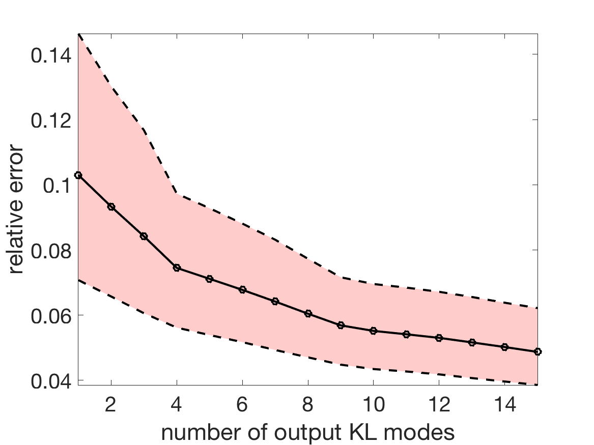
Refer to caption
Refer to caption
Figure 7: Left: The expected value of the error Er​e​lE_{rel} (solid black line) along with the fifth and the ninty fifth percentiles (dashed lines) of Er​e​lE_{rel}. Right: Distribution of Er​e​lE_{rel} computed over the entire domain 𝒟\mathcal{D} (blue) and over the subdomian 𝒟′\mathcal{D}^{\prime} (red).
Refer to caption
Figure 8: Distribution of the error Er​e​lE_{rel} as the number of output KL modes increase from N=1N=1 to N=15N=15.

In Figure 9, we report the distribution of the average pressure along concentric circles of various radii. This shows that the computed surrogate captures statistical properties of the pressure well in different parts of the domain.

Refer to caption
Refer to caption
Refer to caption
Refer to caption
Refer to caption
Refer to caption
Figure 9: Distribution of the pressure averaged over concentric circles of various radii.

5 Concluding remarks

We have presented a distributed active subspace method for scalable surrogate modeling of PDE-governed physical processes with high-dimensional inputs and function valued outputs. To save the modeling efforts spent on function valued outputs, we employ the truncated KL expansion to decouple the spatial dimensions with those of the random variables. As a result, the randomness in outputs is fully represented by scalar valued KL modes. For elliptic PDEs, as observed in the work, a low-rank KL representation of the model output is usually sufficient for an accurate representation. To reduce the dimension of inputs, we construct active subspaces for each of the dominant output KL modes. Since output gradients with respect to the random variables need to be calculated when constructing active subspaces, we develop an adjoint-based framework to ensure that the computational cost does not scale with the input dimension. The method development is complemented by a rigorous mathematical formulation as well as theoretical analysis of errors due to active subspace projection and output KL representation.

We then deploy the distributed active subspace method to conduct surrogate modeling of the pressure field in a biotransport model in tumors with an uncertain permeability field. We demonstrate that a low-rank representation of the pressure field (i.e., output) can be achieved with the truncated KL expansion. The input (i.e., random variables used to represent the uncertain log-permeability field) dimension can be very high (e.g., several hundreds) when the correlation length of the log-permeability field is small. However, we observe that dominant output KL modes admit low (one or two) dimensional active subspaces. We observe that the average relative error between the surrogate model and the PDE solution can be controlled under 5% even when a very low-rank representation of the outputs is employed. We also show that the surrogate models can capture statistical properties of the pressure well in different parts of the domain.

In future work, we will investigate extensions of the distributed active subspace method to surrogate modeling of the time-dependent diffusion and convection-diffusion processes in biological and geological flows. We envision that the truncated KL expansion can be used to extract spatiotemporal coherent structures from the physical process, and the low-dimensional active subspaces can then be constructed for the scalar valued KL modes associated with these structures. This surrogate modeling approach will contribute to cost-effective forward uncertainty quantification, and facilitate solution of inverse problems under uncertainty, such as Bayesian inversion of tissue material properties from medical images.

References

  • (1) Alexanderian, A., Gremaud, P., Smith, R.: Variance-based sensitivity analysis for time-dependent processes. In review (arXiv: https://arxiv.org/abs/1711.08030) (2019)
  • (2) Alexanderian, A., Reese, W., Smith, R.C., Yu, M.: Model input and output dimension reduction using Karhunen–Loève expansions with application to biotransport. ASCE-ASME Journal of Risk and Uncertainty in Engineering Systems Part B: Mechanical Engineering Accepted (2019). https://ui.adsabs.harvard.edu/#abs/2019arXiv190306314A
  • (3) Alexanderian, A., Zhu, L., Salloum, M., Ma, R., Yu, M.: Investigation of biotransport in a tumor with uncertain material properties using a non-intrusive spectral uncertainty quantification method. J. Biomech. Eng. pp. 091006–1–091006–11 (2017)
  • (4) Babuška, I., Nobile, F., Tempone, R.: A stochastic collocation method for elliptic partial differential equations with random input data. SIAM Journal on Numerical Analysis 45(3), 1005–1034 (2007)
  • (5) Clark, W.H.: Tumour progression and the nature of cancer. Br J Cancer 64, 631–44 (1991)
  • (6) Clark, W.H.: Biphasic finite element model of solute transport for direct infusion into nervous tissue. Annals of Biomedical Engineering 35, 2145––2158 (2007)
  • (7) Cleaves, H.L., Alexanderian, A., Guy, H., Smith, R.C., Yu, M.: Derivative-based global sensitivity analysis for models with high-dimensional inputs and functional outputs. arXiv e-prints arXiv:1902.04630 (2019)
  • (8) Constantine, P.: Active Subspaces: Emerging Ideas in Dimension Reduction for Parameter Studies. SIAM, Philadelphia (2015)
  • (9) Constantine, P.G., Diaz, P.: Global sensitivity metrics from active subspaces. Reliability Engineering & System Safety 162, 1–13 (2017)
  • (10) Constantine, P.G., Doostan, A.: Time‐dependent global sensitivity analysis with active subspaces for a lithium ion battery model. Statistical Analysis and Data Mining: The ASA Data Science Journal 10, 243–262 (2017)
  • (11) Constantine, P.G., Dow, E., Wang, Q.: Active subspace methods in theory and practice: applications to kriging surfaces. SIAM Journal on Scientific Computing 36(4), A1500–A1524 (2014)
  • (12) Constantine, P.G., Emory, M., Larsson, J., Iaccarino, G.: Exploiting active subspaces to quantify uncertainty in the numerical simulation of the hyshot ii scramjet. Journal of Computational Physics 302, 1–20 (2015)
  • (13) Debbage, P.: Targeted drugs and nanomedicine: present and future. Current Pharmaceutical Design 15, 153–72 (2009)
  • (14) Doostan, A., Ghanem, R.G., Red-Horse, J.: Stochastic model reduction for chaos representations. Computer Methods in Applied Mechanics and Engineering 196(37-40), 3951–3966 (2007)
  • (15) Elman, H.: Solution algorithms for stochastic galerkin discretizations of differential equations with random data. Handbook of Uncertainty Quantification pp. 1–16 (2017)
  • (16) Friedman, J.: Fast MARS. Tech. Rep. 110, Laboratory for Computational Statistics, Department of Statistics, Stanford University (1993)
  • (17) Gamboa, F., Janon, A., Klein, T., Lagnoux, A., et al.: Sensitivity analysis for multidimensional and functional outputs. Electronic Journal of Statistics 8(1), 575–603 (2014)
  • (18) Ghanem, R.: Probabilistic characterization of transport in heterogeneous media. Computer Methods in Applied Mechanics and Engineering 158(3), 199 – 220 (1998). DOI https://doi.org/10.1016/S0045-7825(97)00250-8. URL http://www.sciencedirect.com/science/article/pii/S0045782597002508
  • (19) Ghanem, R.G., Spanos, P.D.: Stochastic finite elements: a spectral approach. Springer-Verlag, New York (1991). DOI 10.1007/978-1-4612-3094-6. URL http://dx.doi.org/10.1007/978-1-4612-3094-6
  • (20) Graham, I.G., Kuo, F.Y., Nichols, J.A., Scheichl, R., Schwab, C., Sloan, I.H.: Quasi-monte carlo finite element methods for elliptic pdes with lognormal random coefficients. Numerische Mathematik 131(2), 329–368 (2015)
  • (21) Gunzburger, M.: Perspectives in flow control and optimization, vol. 5. Siam (2003)
  • (22) Hsing, T., Eubank, R.: Theoretical foundations of functional data analysis, with an introduction to linear operators. John Wiley & Sons (2015)
  • (23) Iooss, B., Saltelli, A.: Introduction to sensitivity analysis. In: R. Ghanem, D. Higdon, H. Owhadi (eds.) Handbook of uncertainty quantification, pp. 1103–1122. Springer (2017)
  • (24) Jefferson, J., Gilbert, J., Constantine, P., Maxwell, R.: Active subspaces for sensitivity analysis and dimension reduction of an integrated hydrologic model. Computers & Geosciences 83, 127–138 (2015)
  • (25) Ji, W., Wang, J., Zahm, O., Marzouk, Y.M., Yang, B., Ren, Z., Law, C.K.: Shared low-dimensional subspaces for propagating kinetic uncertainty to multiple outputs. Combustion and Flame 190, 146–157 (2018)
  • (26) Kucherenko, S., Iooss, B.: Derivative-based global sensitivity measures. In: R. Ghanem, D. Higdon, H. Owhadi (eds.) Handbook of Uncertainty Quantification. Springer (2017)
  • (27) Le Maıtre, O., Knio, O., Najm, H., Ghanem, R.: Uncertainty propagation using wiener–haar expansions. Journal of computational Physics 197(1), 28–57 (2004)
  • (28) Le Maître, O.P., Knio, O.M.: Spectral methods for uncertainty quantification. Scientific Computation. Springer, New York (2010). DOI 10.1007/978-90-481-3520-2. URL http://dx.doi.org/10.1007/978-90-481-3520-2. With applications to computational fluid dynamics
  • (29) Le Maître, O.P., Reagan, M.T., Najm, H.N., Ghanem, R.G., Knio, O.M.: A stochastic projection method for fluid flow: Ii. random process. Journal of computational Physics 181(1), 9–44 (2002)
  • (30) Loève, M.: Probability theory. I, fourth edn. Springer-Verlag, New York-Heidelberg (1977). Graduate Texts in Mathematics, Vol. 45
  • (31) Lukaczyk, T.W., Palacios, F., Alonso, J.J., Constantine, P.: Active subspaces for shape optimization. In: the 10th AIAA Multidisciplinary Design Optimization Conference. National Harbor, Maryland (2014). AIAA-2014-1171
  • (32) Ma, R., Su, D., Zhu, L.: Multiscale simulation of nanopartical transport in deformable tissue during an infusion process in hyperthermia treatments of cancers. In: W.J. Minkowycz, E. Sparrow, J.P. Abraham (eds.) Nanoparticle Heat Transfer and Fluid Flow, Computational & Physical Processes in Mechanics & Thermal Science Series, vol. 4. CRC Press, Taylor & Francis Group (2012)
  • (33) Mangado, N., Piella, G., Noailly, J., Pons-Prats, J., Ángel González Ballester, M.: Analysis of uncertainty and variability in finite element computational models for biomedical engineering: Characterization and propagation. Front Bioeng Biotechnol. 4, 85 (2016)
  • (34) Matthies, H.G., Keese, A.: Galerkin methods for linear and nonlinear elliptic stochastic partial differential equations. Computer methods in applied mechanics and engineering 194(12-16), 1295–1331 (2005)
  • (35) Prieur, C., Tarantola, S.: Variance-based sensitivity analysis: Theory and estimation algorithms. In: R. Ghanem, D. Higdon, H. Owhadi (eds.) Handbook of Uncertainty Quantification, pp. 1217–1239. Springer (2017)
  • (36) Rasmussen, C.E., Williams, C.: Gaussian processes for machine learning cambridge (2006)
  • (37) Russi, T.M.: Uncertainty quantification with experimental data and complex system models. Ph.D. thesis, University of California, Berkeley (2010)
  • (38) Saad, G., Ghanem, R.: Characterization of reservoir simulation models using a polynomial chaos-based ensemble kalman filter. Water Resources Research 45(4) (2009)
  • (39) Salloum, M., Ma, R., Weeks, D., Zhu, L.: Controlling nanoparticle delivery in magnetic nanoparticle hyperthermia for cancer treatment: experimental study in agarose gel. Int. J. Hyperthermia 24, 337–345 (2008)
  • (40) Sobol, I.: Estimation of the sensitivity of nonlinear mathematical models. Matematicheskoe Modelirovanie 2(1), 112–118 (1990)
  • (41) Sobol, I.: Global sensitivity indices for nonlinear mathematical models and their monte carlo estimates. Mathematics and Computers in Simulation 55(1-3), 271 – 280 (2001)
  • (42) Sobol’, I., Kucherenko, S.: Derivative based global sensitivity measures and their link with global sensitivity indices. Mathematics and Computers in Simulation 79(10), 3009–3017 (2009)
  • (43) Xiu, D., Karniadakis, G.E.: Modeling uncertainty in flow simulations via generalized polynomial chaos. Journal of Computational Physics 187(1), 137 – 167 (2003). DOI https://doi.org/10.1016/S0021-9991(03)00092-5. URL http://www.sciencedirect.com/science/article/pii/S0021999103000925
  • (44) Zahm, O., Constantine, P., Prieur, C., Marzouk, Y.: Gradient-based dimension reduction of multivariate vector-valued functions. arXiv preprint arXiv:1801.07922 (2018)

Appendix A Proofs

Proof of Theorem 3.1:

Note that,

e⁡(𝒙,𝝃)=|∑k=1N(Fk​(𝝃)−Gk​(𝑾k,1T​𝝃))​ϕk​(𝒙)|≤∑k=1N|Fk​(𝝃)−Gk​(𝑾k,1T​𝝃)|​|ϕk​(𝒙)|.e({\mathchoice{\mbox{\boldmath$\displaystyle{x}$}}{\mbox{\boldmath$\textstyle{x}$}}{\mbox{\boldmath$\scriptstyle{x}$}}{\mbox{\boldmath$\scriptscriptstyle{x}$}}},{\mathchoice{\mbox{\boldmath$\displaystyle{\xi}$}}{\mbox{\boldmath$\textstyle{\xi}$}}{\mbox{\boldmath$\scriptstyle{\xi}$}}{\mbox{\boldmath$\scriptscriptstyle{\xi}$}}})=\bigg|\sum_{k=1}^{N}(F_{k}({\mathchoice{\mbox{\boldmath$\displaystyle{\xi}$}}{\mbox{\boldmath$\textstyle{\xi}$}}{\mbox{\boldmath$\scriptstyle{\xi}$}}{\mbox{\boldmath$\scriptscriptstyle{\xi}$}}})-{G}_{k}({\mathchoice{\mbox{\boldmath$\displaystyle{W}$}}{\mbox{\boldmath$\textstyle{W}$}}{\mbox{\boldmath$\scriptstyle{W}$}}{\mbox{\boldmath$\scriptscriptstyle{W}$}}}_{k,1}^{T}{\mathchoice{\mbox{\boldmath$\displaystyle{\xi}$}}{\mbox{\boldmath$\textstyle{\xi}$}}{\mbox{\boldmath$\scriptstyle{\xi}$}}{\mbox{\boldmath$\scriptscriptstyle{\xi}$}}}))\phi_{k}({\mathchoice{\mbox{\boldmath$\displaystyle{x}$}}{\mbox{\boldmath$\textstyle{x}$}}{\mbox{\boldmath$\scriptstyle{x}$}}{\mbox{\boldmath$\scriptscriptstyle{x}$}}})\bigg|\leq\sum_{k=1}^{N}|F_{k}({\mathchoice{\mbox{\boldmath$\displaystyle{\xi}$}}{\mbox{\boldmath$\textstyle{\xi}$}}{\mbox{\boldmath$\scriptstyle{\xi}$}}{\mbox{\boldmath$\scriptscriptstyle{\xi}$}}})-{G}_{k}({\mathchoice{\mbox{\boldmath$\displaystyle{W}$}}{\mbox{\boldmath$\textstyle{W}$}}{\mbox{\boldmath$\scriptstyle{W}$}}{\mbox{\boldmath$\scriptscriptstyle{W}$}}}_{k,1}^{T}{\mathchoice{\mbox{\boldmath$\displaystyle{\xi}$}}{\mbox{\boldmath$\textstyle{\xi}$}}{\mbox{\boldmath$\scriptstyle{\xi}$}}{\mbox{\boldmath$\scriptscriptstyle{\xi}$}}})||\phi_{k}({\mathchoice{\mbox{\boldmath$\displaystyle{x}$}}{\mbox{\boldmath$\textstyle{x}$}}{\mbox{\boldmath$\scriptstyle{x}$}}{\mbox{\boldmath$\scriptscriptstyle{x}$}}})|.

Then,

𝔼​{e¯}\displaystyle\mathbb{E}\{\bar{e}\} =𝔼⁡{∫𝒳∑k=1N|Fk​(𝝃)−Gk​(𝑾k,1T​𝝃)|​|ϕk​(𝒙)|​𝑑x}\displaystyle=\mathbb{E}\bigg\{\int_{\mathcal{X}}\sum_{k=1}^{N}|F_{k}({\mathchoice{\mbox{\boldmath$\displaystyle{\xi}$}}{\mbox{\boldmath$\textstyle{\xi}$}}{\mbox{\boldmath$\scriptstyle{\xi}$}}{\mbox{\boldmath$\scriptscriptstyle{\xi}$}}})-{G}_{k}({\mathchoice{\mbox{\boldmath$\displaystyle{W}$}}{\mbox{\boldmath$\textstyle{W}$}}{\mbox{\boldmath$\scriptstyle{W}$}}{\mbox{\boldmath$\scriptscriptstyle{W}$}}}_{k,1}^{T}{\mathchoice{\mbox{\boldmath$\displaystyle{\xi}$}}{\mbox{\boldmath$\textstyle{\xi}$}}{\mbox{\boldmath$\scriptstyle{\xi}$}}{\mbox{\boldmath$\scriptscriptstyle{\xi}$}}})||\phi_{k}({\mathchoice{\mbox{\boldmath$\displaystyle{x}$}}{\mbox{\boldmath$\textstyle{x}$}}{\mbox{\boldmath$\scriptstyle{x}$}}{\mbox{\boldmath$\scriptscriptstyle{x}$}}})|dx\bigg\}
=∑k=1N(∫𝒳|ϕk​(𝒙)|​𝑑x)​𝔼​{|Fk​(𝝃)−Gk​(𝑾k,1T​𝝃)|}\displaystyle=\sum_{k=1}^{N}\bigg(\int_{\mathcal{X}}|\phi_{k}({\mathchoice{\mbox{\boldmath$\displaystyle{x}$}}{\mbox{\boldmath$\textstyle{x}$}}{\mbox{\boldmath$\scriptstyle{x}$}}{\mbox{\boldmath$\scriptscriptstyle{x}$}}})|dx\bigg)\mathbb{E}\{|F_{k}({\mathchoice{\mbox{\boldmath$\displaystyle{\xi}$}}{\mbox{\boldmath$\textstyle{\xi}$}}{\mbox{\boldmath$\scriptstyle{\xi}$}}{\mbox{\boldmath$\scriptscriptstyle{\xi}$}}})-{G}_{k}({\mathchoice{\mbox{\boldmath$\displaystyle{W}$}}{\mbox{\boldmath$\textstyle{W}$}}{\mbox{\boldmath$\scriptstyle{W}$}}{\mbox{\boldmath$\scriptscriptstyle{W}$}}}_{k,1}^{T}{\mathchoice{\mbox{\boldmath$\displaystyle{\xi}$}}{\mbox{\boldmath$\textstyle{\xi}$}}{\mbox{\boldmath$\scriptstyle{\xi}$}}{\mbox{\boldmath$\scriptscriptstyle{\xi}$}}})|\}
≤∑k=1N[∫𝒳|ϕk​(𝒙)|2​𝑑x]12​[∫𝒳12​𝑑x]12​𝔼​{|Fk​(𝝃)−Gk​(𝑾k,1T​𝝃)2|}1/2≤|𝒳|12​∑k=1Nδk\displaystyle\leq\displaystyle\sum_{k=1}^{N}\left[\int_{\mathcal{X}}|\phi_{k}({\mathchoice{\mbox{\boldmath$\displaystyle{x}$}}{\mbox{\boldmath$\textstyle{x}$}}{\mbox{\boldmath$\scriptstyle{x}$}}{\mbox{\boldmath$\scriptscriptstyle{x}$}}})|^{2}dx\right]^{\frac{1}{2}}\left[\int_{\mathcal{X}}1^{2}dx\right]^{\frac{1}{2}}\mathbb{E}\{|F_{k}({\mathchoice{\mbox{\boldmath$\displaystyle{\xi}$}}{\mbox{\boldmath$\textstyle{\xi}$}}{\mbox{\boldmath$\scriptstyle{\xi}$}}{\mbox{\boldmath$\scriptscriptstyle{\xi}$}}})-{G}_{k}({\mathchoice{\mbox{\boldmath$\displaystyle{W}$}}{\mbox{\boldmath$\textstyle{W}$}}{\mbox{\boldmath$\scriptstyle{W}$}}{\mbox{\boldmath$\scriptscriptstyle{W}$}}}_{k,1}^{T}{\mathchoice{\mbox{\boldmath$\displaystyle{\xi}$}}{\mbox{\boldmath$\textstyle{\xi}$}}{\mbox{\boldmath$\scriptstyle{\xi}$}}{\mbox{\boldmath$\scriptscriptstyle{\xi}$}}})^{2}|\}^{1/2}\leq|\mathcal{X}|^{\frac{1}{2}}\displaystyle\sum_{k=1}^{N}\delta_{k}

where we have used Cauchy–Schwarz inequlity and Lemma 2(a). ∎

Proof of Theorem 3.2:

We have

E¯​(𝝃)=∫𝒳E⁡(𝒙,𝝃)​𝑑x\displaystyle\bar{E}({\mathchoice{\mbox{\boldmath$\displaystyle{\xi}$}}{\mbox{\boldmath$\textstyle{\xi}$}}{\mbox{\boldmath$\scriptstyle{\xi}$}}{\mbox{\boldmath$\scriptscriptstyle{\xi}$}}})=\int_{\mathcal{X}}E({\mathchoice{\mbox{\boldmath$\displaystyle{x}$}}{\mbox{\boldmath$\textstyle{x}$}}{\mbox{\boldmath$\scriptstyle{x}$}}{\mbox{\boldmath$\scriptscriptstyle{x}$}}},{\mathchoice{\mbox{\boldmath$\displaystyle{\xi}$}}{\mbox{\boldmath$\textstyle{\xi}$}}{\mbox{\boldmath$\scriptstyle{\xi}$}}{\mbox{\boldmath$\scriptscriptstyle{\xi}$}}})dx =∫𝒳|f⁡(𝒙,𝝃)−fN​(𝒙,𝝃)+fN​(𝒙,𝝃)−f^N​(𝒙,𝝃)|\displaystyle=\int_{\mathcal{X}}|f({\mathchoice{\mbox{\boldmath$\displaystyle{x}$}}{\mbox{\boldmath$\textstyle{x}$}}{\mbox{\boldmath$\scriptstyle{x}$}}{\mbox{\boldmath$\scriptscriptstyle{x}$}}},{\mathchoice{\mbox{\boldmath$\displaystyle{\xi}$}}{\mbox{\boldmath$\textstyle{\xi}$}}{\mbox{\boldmath$\scriptstyle{\xi}$}}{\mbox{\boldmath$\scriptscriptstyle{\xi}$}}})-f_{N}({\mathchoice{\mbox{\boldmath$\displaystyle{x}$}}{\mbox{\boldmath$\textstyle{x}$}}{\mbox{\boldmath$\scriptstyle{x}$}}{\mbox{\boldmath$\scriptscriptstyle{x}$}}},{\mathchoice{\mbox{\boldmath$\displaystyle{\xi}$}}{\mbox{\boldmath$\textstyle{\xi}$}}{\mbox{\boldmath$\scriptstyle{\xi}$}}{\mbox{\boldmath$\scriptscriptstyle{\xi}$}}})+f_{N}({\mathchoice{\mbox{\boldmath$\displaystyle{x}$}}{\mbox{\boldmath$\textstyle{x}$}}{\mbox{\boldmath$\scriptstyle{x}$}}{\mbox{\boldmath$\scriptscriptstyle{x}$}}},{\mathchoice{\mbox{\boldmath$\displaystyle{\xi}$}}{\mbox{\boldmath$\textstyle{\xi}$}}{\mbox{\boldmath$\scriptstyle{\xi}$}}{\mbox{\boldmath$\scriptscriptstyle{\xi}$}}})-\hat{f}_{N}({\mathchoice{\mbox{\boldmath$\displaystyle{x}$}}{\mbox{\boldmath$\textstyle{x}$}}{\mbox{\boldmath$\scriptstyle{x}$}}{\mbox{\boldmath$\scriptscriptstyle{x}$}}},{\mathchoice{\mbox{\boldmath$\displaystyle{\xi}$}}{\mbox{\boldmath$\textstyle{\xi}$}}{\mbox{\boldmath$\scriptstyle{\xi}$}}{\mbox{\boldmath$\scriptscriptstyle{\xi}$}}})|
≤∫𝒳|f⁡(𝒙,𝝃)−fN​(𝒙,𝝃)|​𝑑x+∫𝒳|fN​(𝒙,𝝃)−f^N​(𝒙,𝝃)|​𝑑x\displaystyle\leq\int_{\mathcal{X}}|f({\mathchoice{\mbox{\boldmath$\displaystyle{x}$}}{\mbox{\boldmath$\textstyle{x}$}}{\mbox{\boldmath$\scriptstyle{x}$}}{\mbox{\boldmath$\scriptscriptstyle{x}$}}},{\mathchoice{\mbox{\boldmath$\displaystyle{\xi}$}}{\mbox{\boldmath$\textstyle{\xi}$}}{\mbox{\boldmath$\scriptstyle{\xi}$}}{\mbox{\boldmath$\scriptscriptstyle{\xi}$}}})-f_{N}({\mathchoice{\mbox{\boldmath$\displaystyle{x}$}}{\mbox{\boldmath$\textstyle{x}$}}{\mbox{\boldmath$\scriptstyle{x}$}}{\mbox{\boldmath$\scriptscriptstyle{x}$}}},{\mathchoice{\mbox{\boldmath$\displaystyle{\xi}$}}{\mbox{\boldmath$\textstyle{\xi}$}}{\mbox{\boldmath$\scriptstyle{\xi}$}}{\mbox{\boldmath$\scriptscriptstyle{\xi}$}}})|dx+\int_{\mathcal{X}}|f_{N}({\mathchoice{\mbox{\boldmath$\displaystyle{x}$}}{\mbox{\boldmath$\textstyle{x}$}}{\mbox{\boldmath$\scriptstyle{x}$}}{\mbox{\boldmath$\scriptscriptstyle{x}$}}},{\mathchoice{\mbox{\boldmath$\displaystyle{\xi}$}}{\mbox{\boldmath$\textstyle{\xi}$}}{\mbox{\boldmath$\scriptstyle{\xi}$}}{\mbox{\boldmath$\scriptscriptstyle{\xi}$}}})-\hat{f}_{N}({\mathchoice{\mbox{\boldmath$\displaystyle{x}$}}{\mbox{\boldmath$\textstyle{x}$}}{\mbox{\boldmath$\scriptstyle{x}$}}{\mbox{\boldmath$\scriptscriptstyle{x}$}}},{\mathchoice{\mbox{\boldmath$\displaystyle{\xi}$}}{\mbox{\boldmath$\textstyle{\xi}$}}{\mbox{\boldmath$\scriptstyle{\xi}$}}{\mbox{\boldmath$\scriptscriptstyle{\xi}$}}})|dx
≤{∫𝒳|f⁡(𝒙,𝝃)−fN​(𝒙,𝝃)|2​𝑑x}1/2​|𝒳|12+e¯​(𝝃)\displaystyle\leq\bigg\{\int_{\mathcal{X}}|f({\mathchoice{\mbox{\boldmath$\displaystyle{x}$}}{\mbox{\boldmath$\textstyle{x}$}}{\mbox{\boldmath$\scriptstyle{x}$}}{\mbox{\boldmath$\scriptscriptstyle{x}$}}},{\mathchoice{\mbox{\boldmath$\displaystyle{\xi}$}}{\mbox{\boldmath$\textstyle{\xi}$}}{\mbox{\boldmath$\scriptstyle{\xi}$}}{\mbox{\boldmath$\scriptscriptstyle{\xi}$}}})-f_{N}({\mathchoice{\mbox{\boldmath$\displaystyle{x}$}}{\mbox{\boldmath$\textstyle{x}$}}{\mbox{\boldmath$\scriptstyle{x}$}}{\mbox{\boldmath$\scriptscriptstyle{x}$}}},{\mathchoice{\mbox{\boldmath$\displaystyle{\xi}$}}{\mbox{\boldmath$\textstyle{\xi}$}}{\mbox{\boldmath$\scriptstyle{\xi}$}}{\mbox{\boldmath$\scriptscriptstyle{\xi}$}}})|^{2}dx\bigg\}^{1/2}|\mathcal{X}|^{\frac{1}{2}}+\bar{e}({\mathchoice{\mbox{\boldmath$\displaystyle{\xi}$}}{\mbox{\boldmath$\textstyle{\xi}$}}{\mbox{\boldmath$\scriptstyle{\xi}$}}{\mbox{\boldmath$\scriptscriptstyle{\xi}$}}})
={∑k=N+1∞Fk​(𝝃)2}1/2​|𝒳|12+e¯​(𝝃).\displaystyle=\bigg\{\sum_{k=N+1}^{\infty}F_{k}({\mathchoice{\mbox{\boldmath$\displaystyle{\xi}$}}{\mbox{\boldmath$\textstyle{\xi}$}}{\mbox{\boldmath$\scriptstyle{\xi}$}}{\mbox{\boldmath$\scriptscriptstyle{\xi}$}}})^{2}\bigg\}^{1/2}|\mathcal{X}|^{\frac{1}{2}}+\bar{e}({\mathchoice{\mbox{\boldmath$\displaystyle{\xi}$}}{\mbox{\boldmath$\textstyle{\xi}$}}{\mbox{\boldmath$\scriptstyle{\xi}$}}{\mbox{\boldmath$\scriptscriptstyle{\xi}$}}}).

Now we consider

𝔼​{E¯​(𝝃)}\displaystyle\mathbb{E}\{\bar{E}({\mathchoice{\mbox{\boldmath$\displaystyle{\xi}$}}{\mbox{\boldmath$\textstyle{\xi}$}}{\mbox{\boldmath$\scriptstyle{\xi}$}}{\mbox{\boldmath$\scriptscriptstyle{\xi}$}}})\} ≤𝔼⁡({∑k=N+1∞Fk​(𝝃)2}1/2)​|𝒳|12+𝔼⁡{e¯​(𝝃)}\displaystyle\leq\mathbb{E}\Bigg(\bigg\{\sum_{k=N+1}^{\infty}F_{k}({\mathchoice{\mbox{\boldmath$\displaystyle{\xi}$}}{\mbox{\boldmath$\textstyle{\xi}$}}{\mbox{\boldmath$\scriptstyle{\xi}$}}{\mbox{\boldmath$\scriptscriptstyle{\xi}$}}})^{2}\bigg\}^{1/2}\Bigg)|\mathcal{X}|^{\frac{1}{2}}+\mathbb{E}\{\bar{e}({\mathchoice{\mbox{\boldmath$\displaystyle{\xi}$}}{\mbox{\boldmath$\textstyle{\xi}$}}{\mbox{\boldmath$\scriptstyle{\xi}$}}{\mbox{\boldmath$\scriptscriptstyle{\xi}$}}})\}
≤|𝒳|12​[𝔼⁡({∑k=N+1∞Fk​(𝝃)2}1/2)+∑k=1Nδk]≤|𝒳|12​[𝔼​(∑k=N+1∞Fk​(𝝃)2)1/2+∑k=1Nδk].\displaystyle\leq|\mathcal{X}|^{\frac{1}{2}}\Bigg[\mathbb{E}\Bigg(\bigg\{\sum_{k=N+1}^{\infty}F_{k}({\mathchoice{\mbox{\boldmath$\displaystyle{\xi}$}}{\mbox{\boldmath$\textstyle{\xi}$}}{\mbox{\boldmath$\scriptstyle{\xi}$}}{\mbox{\boldmath$\scriptscriptstyle{\xi}$}}})^{2}\bigg\}^{1/2}\Bigg)+\sum_{k=1}^{N}\delta_{k}\Bigg]\leq|\mathcal{X}|^{\frac{1}{2}}\Bigg[\mathbb{E}\Bigg(\sum_{k=N+1}^{\infty}F_{k}({\mathchoice{\mbox{\boldmath$\displaystyle{\xi}$}}{\mbox{\boldmath$\textstyle{\xi}$}}{\mbox{\boldmath$\scriptstyle{\xi}$}}{\mbox{\boldmath$\scriptscriptstyle{\xi}$}}})^{2}\Bigg)^{1/2}+\sum_{k=1}^{N}\delta_{k}\Bigg].

Note that 𝔼⁡(∑k=N+1∞Fk​(𝝃)2)=∑k=N+1∞𝔼⁡(Fk​(𝝃)2)=∑k=N+1∞λk​(Cf)\mathbb{E}\Bigg(\sum_{k=N+1}^{\infty}F_{k}({\mathchoice{\mbox{\boldmath$\displaystyle{\xi}$}}{\mbox{\boldmath$\textstyle{\xi}$}}{\mbox{\boldmath$\scriptstyle{\xi}$}}{\mbox{\boldmath$\scriptscriptstyle{\xi}$}}})^{2}\Bigg)=\sum_{k=N+1}^{\infty}\mathbb{E}\big(F_{k}({\mathchoice{\mbox{\boldmath$\displaystyle{\xi}$}}{\mbox{\boldmath$\textstyle{\xi}$}}{\mbox{\boldmath$\scriptstyle{\xi}$}}{\mbox{\boldmath$\scriptscriptstyle{\xi}$}}})^{2}\big)=\sum_{k=N+1}^{\infty}\lambda_{k}(C_{f}). Therefore, we have our desired result

𝔼​{E¯​(𝝃)}≤|𝒳|12​[(∑k=N+1∞λk​(Cf))1/2+∑k=1Nδk]=|𝒳|12​[(∑k=N+1∞λk​(Cf))1/2+∑k=1N(∑j=rk+1Npλj​(𝐒k))1/2]..\begin{aligned} \mathbb{E}\{\bar{E}({\mathchoice{\mbox{\boldmath$\displaystyle{\xi}$}}{\mbox{\boldmath$\textstyle{\xi}$}}{\mbox{\boldmath$\scriptstyle{\xi}$}}{\mbox{\boldmath$\scriptscriptstyle{\xi}$}}})\}&\leq|\mathcal{X}|^{\frac{1}{2}}\Bigg[\Bigg(\sum_{k=N+1}^{\infty}\lambda_{k}(C_{f})\Bigg)^{1/2}+\sum_{k=1}^{N}\delta_{k}\Bigg]\\ &=|\mathcal{X}|^{\frac{1}{2}}\Bigg[\Bigg(\sum_{k=N+1}^{\infty}\lambda_{k}(C_{f})\Bigg)^{1/2}+\sum_{k=1}^{N}\left(\sum_{j=r_{k}+1}^{N_{p}}\lambda_{j}(\mathbf{{S}}_{k})\right)^{1/2}\Bigg].\end{aligned}.

∎