Statistical analysis of the azimuthal asymmetry in the leptoproduction in unpolarized collisions
Abstract
In this paper, we study the azimuthal asymmetry in the leptoproduction in unpolarized collisions. There are two independent azimuthal asymmetry modulations, namely and , where is the azimuthal angle of the lepton scattering plane with respect to the hadron-interacting plane. We calculate the two modulations as functions of four kinematic variables, and find that they provide a very good laboratory to distinguish several models describing the heavy quarkonium production, including the color-singlet (CS) model, the nonrelativistic QCD (NRQCD) associated with the dominance picture, and the NRQCD in which the values of all the three color-octet (CO) long-distance matrix elements are of the same order. In order to make definite conclusions, we restrict our calculation in a specific kinematic region, where the CS and CO mechanisms can be distinguished by scrutinizing the values of the modulation, while the dominance picture can be tested by measuring the values of the modulation. Calculating their values and carrying out a meticulous statistical analysis, we find that at an integrated luminosity , the statistical uncertainties of the two quantities are small enough to tell the three models apart. When this experiment is implemented at the future colliders such as the EIC, crucial information for the production mechanism might be discovered.
Keywords
azimuthal asymmetry, production1 Introduction
It has not been realized that the transverse polarization and transverse momentum effects in nucleons could be significant until the first measurement of inclusive pion hadroproduction was carried out at Argonne synchrotron Dick:1975ty; Klem:1976ui; Dragoset:1978gg, the results of which were later confirmed by Fermilab Bunce:1976yb at a slightly higher colliding energy. In order to understand the unexpected large transverse spin asymmetries observed in those experiments, various theoretical mechanisms and new structure functions were proposed, among which are there the well-known Sivers effect Sivers:1989cc; Sivers:1990fh along with a new function, the Sivers function, describing the azimuthal asymmetry of unpolarized quarks in polarized hadrons, and Collins effect Collins:1992kk; Collins:1993kq, considering the different fragmenting probabilities of transversely polarized partons to hadrons with transverse momentum along different directions. Since this century, the transverse spin effects have been studied experimentally in semi-inclusive deep-inelastic scattering (SIDIS). In 2004, HERMES Airapetian:2004tw and COMPASS Alexakhin:2005iw; Ageev:2006da published their measurements of the single-spin asymmetry in the collisions of leptons off polarized proton and deuteron targets. One of the main advantages of SIDIS is that the transverse spin and transverse momentum effects are not mixed, as in hadroproduction; they result in different azimuthal asymmetry modulations. Another interesting feature of SIDIS is that, even with unpolarized targets, there also exist two types of azimuthal asymmetry modulations, namely the and modulations, where is the azimuthal angle for the observed final-state hadron with respect to the virtual-photon-target beam. A few years ago, HERMES Airapetian:2012yg and COMPASS Adolph:2014pwc collaborations presented the data for the azimuthal distributions of hadrons produced in deep inelastic scattering off unpolarized targets and found nonzero and azimuthal asymmetry modulations. These modulations arise as long as the momenta of the final-state hadrons have transverse components, which may originate from either the intrinsic transverse motion of partons inside the targets, or the hard emission of the final-state hadrons. The former one was first studied by Cahn Cahn:1978se; Cahn:1989yf and thus is called the Cahn effect. Cahn effect dominates in low region, while in high region, the real emission plays a more important role.
The azimuthal asymmetries in unpolarized SIDIS not only provide essential information for the transverse insight of nucleons, but also open a window for the study of hadron production mechanisms, e.g. the heavy quarkonium production mechanism. Although heavy quarkonia have very simple structure, their production mechanism is still unknown. Nonrelativistic QCD (NRQCD) Bodwin:1994jh, which separates the perturbatively calculable short-distance coefficients (SDCs) from the process-independent long-distance matrix elements (LDMEs), is one of the most successful theories describing the quarkonium productions and decays. However it confronted a lot of difficulties and challenges in the past two decades. The most famous one of those is the polarization puzzle. In the last decade, many processes have been calculated up to QCD next-to-leading order (NLO), including the Zhang:2005cha; Zhang:2006ay; Gong:2007db; Gong:2008ce; Ma:2008gq; Gong:2009kp; Gong:2009ng; Zhang:2009ym; Wang:2011qg; Feng:2017bdu; Jiang:2018wmv and the Gong:2016jiq production in annihilation, the photoproduction in Klasen:2004tz and Kramer:1995nb; Maltoni:1997pt; Artoisenet:2009xh; Chang:2009uj; Li:2009fd; Butenschoen:2009zy; Butenschoen:2011ks; Bodwin:2015yma collisions, the Campbell:2007ws; Gong:2008sn; Gong:2008hk; Gong:2008ft; Ma:2010yw; Butenschoen:2010rq; Ma:2010jj; Butenschoen:2011yh; Butenschoen:2012px; Chao:2012iv; Gong:2012ug; Gong:2012ah; Lansberg:2013qka; Li:2014ava; Bodwin:2014gia; Lansberg:2014swa; Shao:2014yta; Sun:2015pia; Bodwin:2015iua; Feng:2018cai, Butenschoen:2014dra; Han:2014jya; Zhang:2014ybe; Lansberg:2017ozx; Feng:2019zmn, and Ma:2010vd; Li:2011yc; Shao:2012fs; Shao:2014fca; Jia:2014jfa hadroproduction, and the production in deep-inelastic scattering (DIS) Sun:2017wxk. As a noteworthy progress, the measurement of the production Barsuk:2012ic; Aaij:2014bga stimulated a lot of theoretical works Butenschoen:2014dra; Han:2014jya; Zhang:2014ybe; Gong:2016jiq; Lansberg:2017ozx; Feng:2019zmn; Zhang:2019wxo. Unfortunately, neither a set of globally working LDMEs has been found, nor the importance of the color-octet (CO) mechanism has been demonstrated. We refer the readers to Reference Lansberg:2017ozx as a state-of-the-art review. Azimuthal asymmetry in the production in DIS can serve as an alternative test of NRQCD. As we will see later, in some specific kinematic regions, the azimuthal asymmetry can distinguish different production channels. Based on statistical analysis, we propose a practical strategy to verify the CO mechanism and fix the corresponding LDMEs.
2 The azimuthal asymmetry in the leptoproduction
2.1 The calculation of the cross sections
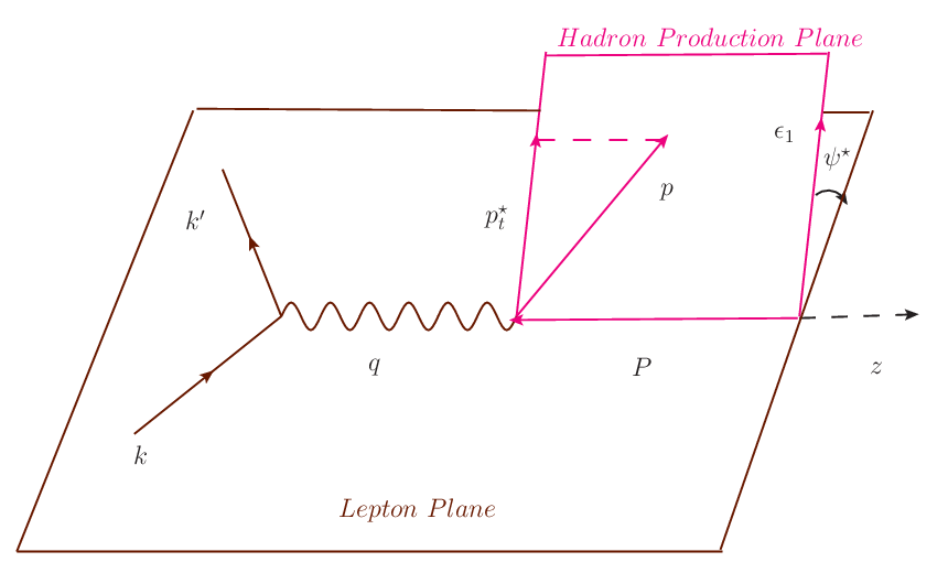
In electron-proton collisions,
| (1) |
which, in general, can be reduced into the virtual-photon-proton fusion process as
| (2) |
Here, represents the proton remnant. , , , , , and are the momenta of the initial-state electron, proton, and virtual photon, the final-state electron, the , and the proton remnant. Usually, we use the following invariants to describe the kinematics of this process,
| (3) |
the first two of which can be replaced by the following two dimensionless invariants,
| (4) |
as long as the invariant colliding energy squared, , is given. Here, is the well-known Bjorken-, and is named the elasticity coefficient.
To study the azimuthal effects, we adopt such frames in which the virtual photon and the proton beams are along the and anti- directions, respectively, as illustrated in Figure 1. The azimuthal angle of the final-state is then defined with respect to the virtual-photon-proton beams. In such frames, the physical quantities are always labelled by a superscript , in order to distinguish from those in laboratory frames. Since the laboratory frame is not concerned in this paper, we just omit the superscript . In addition to the invariants, , , and (or equivalently, , , and ), we need two more quantities, the transverse momentum of the final-state , , and its azimuthal angle, , to sufficiently describe the kinematics of the leptoproduction process. We define two dimensionless quantities,
| (5) |
where is the mass, so that the SIDIS process can be described by six dimensionless variables, , , , , , and . Having all these kinematic variables, we can write down the hadron production cross section in unpolarized SIDIS as (see e.g. Reference Zhang:2017dia)
| (6) |
where is the electromagnetic fine-structure constant, is the hadronic tensor integrated over the phase-space of the final-state hadrons other than the , and the normalized leptonic tensor, , is defined as
| (7) |
If only one final-state hadron is observed, the leptonic tensor, , can be decomposed into the linear combination of four simpler tensors, factorizing all the azimuthally dependent terms into the corresponding coefficients as
| (8) |
where
| (9) |
and
| (10) |
Here, is defined as
| (11) |
where the proton mass has been neglected. Substituting Equation (9) into Equation (8) and taking into account the current-conserving equation,
| (12) |
we can rewrite the normalized leptonic tensor in a form that is more convenient for computation as
| (13) |
where
| (14) |
If we define
| (15) |
these ’s can be expressed in a more compact form as
| (16) |
In collinear factorization, the protons interact with the virtual photons via the on-shell partons, and thus, the hadronic tensor, , can be further factorized as the summation of the parton-level hadronic tensors convoluted with the parton distribution functions (PDFs). For production, there is only one parton-level process at QCD LO, i.e.
| (17) |
while for the production of the three color-octet states, namely , , and , there are two parton-level processes at QCD LO, they are
| (18) |
Here, represents , , or . Denoting the squared amplitudes of the above processes as , where and are the Lorentz indices for the virtual photons in the amplitude and its complex conjugate, respectively, can be written as
| (19) |
where runs over the four intermediate states, is the synthesized initial-state averaging factor, is the fraction of the proton momentum taken by the parton, is the corresponding PDF, is the LDME for an intermediate state, , producing a , and is defined as
| (20) |
Here, and are the momenta of the initial- and final-state parton, respectively, and has been implemented. Having and integrated over, can be further simplified as (see e.g. Reference Sun:2017nly)
| (21) |
Having Equation (21), Equation (6) then leads to
| (22) |
Note that in Equation (22) the value of has been fixed by the 0-th dimension of the -function at
| (23) |
To write the cross section in a more compact form, we define
| (24) |
The cross section can correspondingly be expressed as
| (25) |
Since can be easily evaluated via Feynman diagrams, we have been equipped with all the elements needed in Equation (22) for calculating the leptoproduction cross sections.
2.2 The calculation of the azimuthal asymmetry modulations


Since and the tensor basis in Equation (13) are all restricted in the hadronic plane, i.e. they are independent of the azimuthal angle , the azimuthal asymmetry modulations appear only in the coefficients in the leptonic tensor expansions, namely in ’s. In any case, the cross section can be written in the following form,
| (26) |
Therein, and are two independent azimuthal asymmetry modulations. They are functions of , , , and . Explicitly, they can be accessed via the following equations,
| (27) |
Since the four intermediate states contribute independently, one can study the azimuthal asymmetry originated from them respectively. In this sense, the cross section can be written in the following form as
| (28) |
In the next section as we present their numerical results, we just omit the superscript .


Sometimes, it is useful to study the integrated cross sections, the azimuthal asymmetry modulations should be redefined accordingly. When we observe the azimuthal asymmetry modulations in a specific kinematic region, e.g , where is a 4-dimensional area in the --- space, the corresponding azimuthal asymmetry modulations in the region , and , are defined according to the following equation,
| (29) |
They can also be expressed in the following explicit form as
| (30) |
3 Numerical results and phenomenological analysis


In our numerical calculation, we dopt the following parameter choices. The charm quark mass, , is fixed at one half of the mass, which is approximated to . The colliding energy is chosen as to accord with the HERA experiment. To evaluate the parton distributions in protons, we employ the GRV PDF given in Reference Gluck:1994uf. Therein, the factorization scale is set to be .


With the above parameter choices, we present the values of in Figure 2, 3, 4, and those of in Figure 5, 6, 7, for individual states. The dependence of the azimuthal asymmetry modulations are presented for any combination of the following parameter choices, 0.005, 0.05, 0.5, 0.1, 0.4, 0.7, and =0.3, 0.6, 0.9. The value of ranges from 0.00001 to 0.001, corresponding to to .


As an inspiring result, the values of the azimuthal asymmetry modulations for the four states are remarkably distinguished in some of these kinematic regions. To tell the CS and CO channels apart, we can measure at , and , where the values of for all the three CO states lie around 0, while those for the CS state is as large as 1. If, as argued in some papers, the production is dominated by the CS channel, the value of in this region should coincide with the solid curve presented in the plot at the lower right corner in Figure 4. However, this strategy is not feasible because in large- region, the cross sections are so small that no enough events can be produced in this region to perform reasonable analysis. Fortunately, this problem can be amended by including the small- region, where although the CS and channels cannot be distinguished, the CS and CO mechanisms are still distinguishable as the channel is greatly suppressed in leptoproduction, For this reason, we perform our analysis in the region and , in which the value of is generally larger than and the validity of the perturbative expansion is guaranteed.


Another interesting feature of our numerical results is that the channel can also be well distinguished in some kinematic regions. For , , and , the value of for is almost -1, while that for all the other three states is almost 0. Since most of the extractions of the CO LDMEs lead to the same picture, i.e. the LDME is at least one order of magnitude greater than the other two, which however is not consistent with the NRQCD scaling, this feature provides a perfect laboratory to test the dominance picture. If the leptoproduction is also dominated by the channel, we should observe the value of at almost -1 in this kinematic region. Since at larger value of , the cross sections are very small, we can carry out the analysis in the same kinematic region as in the above paragraph, namely and .
In order to draw up a practical strategy for the experimental measurement, we need to calculate the number of events assuming a luminosity, and analyse the systematic uncertainties. For this purpose, we need to specify the value of the renormalization scale , the strong coupling constant , and electromagnetic fine structure constant . The value of in our calculation is given by . The running of follows the following equation,
| (31) |
where at , is given by . It is easy to verify that at the boson mass , the value of is approximately 0.130. The electromagnetic fine structure constant is adopted.
In the following, we carry out our study in the kinematic region, say and . Due to the limit of the capability of the detectors, we further constrain the value of and in the region and . In the following, we denote this kinematic region as . This configuration correspond to , , and . The lower bound of can be easily obtained as , which is a moderate value to neglect the gluon saturation effects.
Integrating over , , , and in the region , we obtain the cross sections contributed from the four channels as
| (32) |
where
| (33) |
and
| (34) |
As expected, the CS and CO channels can be well separated by measuring , while the channel can be distinguished by studying . Although the short-distance coefficient for the channel is almost twice of that for the CS one, the cross section for this channel, however, is negligible due to a much smaller LDME which is suppressed by two orders of magnitude relative to the CS one. On the experiment side, the events are collected in bins of . The azimuthal modulations thus can be extracted by fitting the data to Equation (29), where linear regression is always used as a standard technique. Since the quantities that we are interested in are ratios, most of the systematic uncertainties are cancelled when doing the data analysis. As a result, we consider only the statistical uncertainty in the following. In our analysis, the range, , of is divided into 12 equidistant bins, namely , , . The integral over of the three modulations, 1, , and , in each bin are calculated, and make up three vectors each of which consists of 12 elements. Explicitly, they are
| (35) |
It is easy to verify that the three vectors are linearly independent and not correlated.
If the leptoproduction is dominated by the CS mechanism, the integrated cross section in the region can be expressed as
| (36) |
where
| (37) |
is employed Eichten:1995ch. Assuming the integrated luminosity at the future collider is , we can construct the similar vector, as in the above paragraph, for this distribution as
| (38) |
each element of which is expectation of the number of events collected in the corresponding bin. This number, denoted as , obey Gaussian distribution, the standard error of which can be obtained as the square root of . Denoting the probability density function of the number of events in each bin as , , we fit to the following equation,
| (39) |
We can then obtain the expectation values of , , and , for each combination of the values of . These expectation values thus have a probability density . Then we can calculate the expectation value of the coefficients in Equation (32) for each combination of , and the probability density function with respect to , , and . It is easy to demonstrate that , , and also obey Gaussian distribution, and there expectation values and standard errors are , , , , and , , respectively. Apparently, the expectation values obtained here agree with Equation (36). The uncertainties for and can be obtained as
| (40) |
If the CO parts are not negligible, we need to sum over their contributions. Employing the LDMEs obtained in References Zhang:2014ybe; Sun:2015pia, which are given below,
| (41) |
the cross section can be expressed as
| (42) |
This equation leads to . It is easy to see that this number is well separated from that led to by the CS model in the sense of the uncertainty given in Equation (40).
In the rest of this paper, we will demonstrate that the azimuthal asymmetry in the leptoproduction can also distinguish the LDMEs that are consistent with the dominance picture. Taking those given in Reference Chao:2012iv as an example, say
| (43) |
The cross section for the production in the region can be expressed as
| (44) |
Using the same analysis strategy, we can obtain
| (45) |
Since with the LDMEs given in Equation (41), the value of is -0.0155, it is obvious that one can distinguish the two sets of LDMEs by scrutinize the value of .
4 Summary
In this paper, we calculated the azimuthal asymmetry modulations in the leptoproduction, namely and defined in Equation (27), as functions of , , , and . By scrutinizing their behaviours, we find that the CS and CO mechanisms can be well distinguished through the measurement of the values of . Further, the dominance picture can also be tested by measuring the values of . Restricted in the region, , , , and , we carried out the calculation of the differential cross sections with respect to the azimuthal angle for three models, and found that they lead to clearly different values of the azimuthal-asymmetry modulations. Having applied rigorous statistical analysis, we found that at the integrated luminosity , the statistical uncertainties of and are small enough to tell the three models apart. As a conclusion, the azimuthal asymmetry in the leptoproduction provides a good laboratory for the study of the quarkonium production mechanisms. We suggest that this experiment be implemented at the future colliders such as the EIC.
Acknowledgements.
We thank Zhan Sun for his contribution at the early stage. This work is supported by the National Natural Science Foundation of China (Grant Nos. 11605144, 11747037). Y.-P. Y. acknowledges support from SUT and the Office of the Higher Education Commission under the National Research Universities project of Thailand.References
- (1) L. Dick et al., Spin Effects in the Inclusive Reactions pi+- Polarized p –> pi+- Anything at 8-GeV/c, Phys. Lett. 57B (1975) 93–96.
- (2) R. D. Klem, J. E. Bowers, H. W. Courant, H. Kagan, M. L. Marshak, E. A. Peterson, K. Ruddick, W. H. Dragoset, and J. B. Roberts, Measurement of Asymmetries of Inclusive Pion Production in Proton Proton Interactions at 6-GeV/c and 11.8-GeV/c, Phys. Rev. Lett. 36 (1976) 929–931.
- (3) W. H. Dragoset, J. B. Roberts, J. E. Bowers, H. W. Courant, H. Kagan, M. L. Marshak, E. A. Peterson, K. Ruddick, and R. D. Klem, Asymmetries in Inclusive Proton-Nucleon Scattering at 11.75-GeV/c, Phys. Rev. D18 (1978) 3939–3954.
- (4) G. Bunce et al., Lambda0 Hyperon Polarization in Inclusive Production by 300-GeV Protons on Beryllium., Phys. Rev. Lett. 36 (1976) 1113–1116.
- (5) D. W. Sivers, Single Spin Production Asymmetries from the Hard Scattering of Point-Like Constituents, Phys. Rev. D41 (1990) 83.
- (6) D. W. Sivers, Hard scattering scaling laws for single spin production asymmetries, Phys. Rev. D43 (1991) 261–263.
- (7) J. C. Collins, Fragmentation of transversely polarized quarks probed in transverse momentum distributions, Nucl. Phys. B396 (1993) 161–182, [hep-ph/9208213].
- (8) J. C. Collins, S. F. Heppelmann, and G. A. Ladinsky, Measuring transversity densities in singly polarized hadron hadron and lepton - hadron collisions, Nucl. Phys. B420 (1994) 565–582, [hep-ph/9305309].
- (9) HERMES Collaboration, A. Airapetian et al., Single-spin asymmetries in semi-inclusive deep-inelastic scattering on a transversely polarized hydrogen target, Phys. Rev. Lett. 94 (2005) 012002, [hep-ex/0408013].
- (10) COMPASS Collaboration, V. Yu. Alexakhin et al., First measurement of the transverse spin asymmetries of the deuteron in semi-inclusive deep inelastic scattering, Phys. Rev. Lett. 94 (2005) 202002, [hep-ex/0503002].
- (11) COMPASS Collaboration, E. S. Ageev et al., A New measurement of the Collins and Sivers asymmetries on a transversely polarised deuteron target, Nucl. Phys. B765 (2007) 31–70, [hep-ex/0610068].
- (12) HERMES Collaboration, A. Airapetian et al., Azimuthal distributions of charged hadrons, pions, and kaons produced in deep-inelastic scattering off unpolarized protons and deuterons, Phys. Rev. D87 (2013), no. 1 012010, [arXiv:1204.4161].
- (13) COMPASS Collaboration, C. Adolph et al., Measurement of azimuthal hadron asymmetries in semi-inclusive deep inelastic scattering off unpolarised nucleons, Nucl. Phys. B886 (2014) 1046–1077, [arXiv:1401.6284].
- (14) R. N. Cahn, Azimuthal Dependence in Leptoproduction: A Simple Parton Model Calculation, Phys. Lett. 78B (1978) 269–273.
- (15) R. N. Cahn, Critique of Parton Model Calculations of Azimuthal Dependence in Leptoproduction, Phys. Rev. D40 (1989) 3107–3110.
- (16) G. T. Bodwin, E. Braaten, and G. P. Lepage, Rigorous QCD analysis of inclusive annihilation and production of heavy quarkonium, Phys. Rev. D51 (1995) 1125–1171, [hep-ph/9407339]. [Erratum: Phys. Rev.D55,5853(1997)].
- (17) Y.-J. Zhang, Y.-j. Gao, and K.-T. Chao, Next-to-leading order QCD correction to at GeV, Phys. Rev. Lett. 96 (2006) 092001, [hep-ph/0506076].
- (18) Y.-J. Zhang and K.-T. Chao, Double charm production at B factories with next-to-leading order QCD correction, Phys. Rev. Lett. 98 (2007) 092003, [hep-ph/0611086].
- (19) B. Gong and J.-X. Wang, QCD corrections to plus production in annihilation at =10.6GeV, Phys. Rev. D77 (2008) 054028, [arXiv:0712.4220].
- (20) B. Gong and J.-X. Wang, QCD corrections to double production in annihilation at =10.6GeV, Phys. Rev. Lett. 100 (2008) 181803, [arXiv:0801.0648].
- (21) Y.-Q. Ma, Y.-J. Zhang, and K.-T. Chao, QCD correction to at B Factories, Phys. Rev. Lett. 102 (2009) 162002, [arXiv:0812.5106].
- (22) B. Gong and J.-X. Wang, Next-to-Leading-Order QCD Corrections to at the B Factories, Phys. Rev. Lett. 102 (2009) 162003, [arXiv:0901.0117].
- (23) B. Gong and J.-X. Wang, Next-to-leading-order QCD corrections to at the B factories, Phys. Rev. D80 (2009) 054015, [arXiv:0904.1103].
- (24) Y.-J. Zhang, Y.-Q. Ma, K. Wang, and K.-T. Chao, QCD radiative correction to color-octet inclusive production at B Factories, Phys. Rev. D81 (2010) 034015, [arXiv:0911.2166].
- (25) K. Wang, Y.-Q. Ma, and K.-T. Chao, QCD corrections to (J=0,1,2) at B Factories, Phys. Rev. D84 (2011) 034022, [arXiv:1107.2646].
- (26) Y. Feng, Z. Sun, and H.-F. Zhang, Is the color-octet mechanism consistent with the double production measurement at B-factories?, Eur. Phys. J. C77 (2017), no. 4 221, [arXiv:1701.00969].
- (27) Y. Jiang and Z. Sun, Further studies on the exclusive productions of ( ) via annihilation at the factories, Eur. Phys. J. C78 (2018), no. 11 892, [arXiv:1809.09071].
- (28) Q.-R. Gong, Z. Sun, H.-F. Zhang, and X.-M. Mo, production associated with light hadrons at the B-factories and the future Super B-factories, Eur. Phys. J. C76 (2016), no. 9 518, [arXiv:1606.08317].
- (29) M. Klasen, B. A. Kniehl, L. N. Mihaila, and M. Steinhauser, plus jet associated production in two-photon collisions at next-to-leading order, Nucl. Phys. B713 (2005) 487–521, [hep-ph/0407014].
- (30) M. Kramer, QCD corrections to inelastic photoproduction, Nucl. Phys. B459 (1996) 3–50, [hep-ph/9508409].
- (31) F. Maltoni, M. L. Mangano, and A. Petrelli, Quarkonium photoproduction at next-to-leading order, Nucl. Phys. B519 (1998) 361–393, [hep-ph/9708349].
- (32) P. Artoisenet, J. M. Campbell, F. Maltoni, and F. Tramontano, production at HERA, Phys. Rev. Lett. 102 (2009) 142001, [arXiv:0901.4352].
- (33) C.-H. Chang, R. Li, and J.-X. Wang, polarization in photo-production up-to the next-to-leading order of QCD, Phys. Rev. D80 (2009) 034020, [arXiv:0901.4749].
- (34) R. Li and K.-T. Chao, Photoproduction of in association with a c anti-c pair, Phys. Rev. D79 (2009) 114020, [arXiv:0904.1643].
- (35) M. Butenschoen and B. A. Kniehl, Complete next-to-leading-order corrections to photoproduction in nonrelativistic quantum chromodynamics, Phys. Rev. Lett. 104 (2010) 072001, [arXiv:0909.2798].
- (36) M. Butenschoen and B. A. Kniehl, Probing nonrelativistic QCD factorization in polarized photoproduction at next-to-leading order, Phys. Rev. Lett. 107 (2011) 232001, [arXiv:1109.1476].
- (37) G. T. Bodwin, H. S. Chung, U.-R. Kim, and J. Lee, Fragmentation contributions to J/ψ photoproduction at HERA, Phys. Rev. D92 (2015), no. 7 074042, [arXiv:1504.06019].
- (38) J. M. Campbell, F. Maltoni, and F. Tramontano, QCD corrections to J/psi and Upsilon production at hadron colliders, Phys. Rev. Lett. 98 (2007) 252002, [hep-ph/0703113].
- (39) B. Gong and J.-X. Wang, Next-to-leading-order QCD corrections to polarization at Tevatron and Large-Hadron-Collider energies, Phys. Rev. Lett. 100 (2008) 232001, [arXiv:0802.3727].
- (40) B. Gong and J.-X. Wang, QCD corrections to polarization of and at Tevatron and LHC, Phys. Rev. D78 (2008) 074011, [arXiv:0805.2469].
- (41) B. Gong, X. Q. Li, and J.-X. Wang, QCD corrections to production via color octet states at Tevatron and LHC, Phys. Lett. B673 (2009) 197–200, [arXiv:0805.4751]. [Erratum: Phys. Lett.B693,612(2010)].
- (42) Y.-Q. Ma, K. Wang, and K.-T. Chao, production at the Tevatron and LHC at in nonrelativistic QCD, Phys. Rev. Lett. 106 (2011) 042002, [arXiv:1009.3655].
- (43) M. Butenschoen and B. A. Kniehl, Reconciling production at HERA, RHIC, Tevatron, and LHC with NRQCD factorization at next-to-leading order, Phys. Rev. Lett. 106 (2011) 022003, [arXiv:1009.5662].
- (44) Y.-Q. Ma, K. Wang, and K.-T. Chao, A complete NLO calculation of the and production at hadron colliders, Phys. Rev. D84 (2011) 114001, [arXiv:1012.1030].
- (45) M. Butenschoen and B. A. Kniehl, World data of production consolidate NRQCD factorization at NLO, Phys. Rev. D84 (2011) 051501, [arXiv:1105.0820].
- (46) M. Butenschoen and B. A. Kniehl, polarization at Tevatron and LHC: Nonrelativistic-QCD factorization at the crossroads, Phys. Rev. Lett. 108 (2012) 172002, [arXiv:1201.1872].
- (47) K.-T. Chao, Y.-Q. Ma, H.-S. Shao, K. Wang, and Y.-J. Zhang, Polarization at Hadron Colliders in Nonrelativistic QCD, Phys. Rev. Lett. 108 (2012) 242004, [arXiv:1201.2675].
- (48) B. Gong, L.-P. Wan, J.-X. Wang, and H.-F. Zhang, Polarization for Prompt and Production at the Tevatron and LHC, Phys. Rev. Lett. 110 (2013), no. 4 042002, [arXiv:1205.6682].
- (49) B. Gong, J.-P. Lansberg, C. Lorce, and J. Wang, Next-to-leading-order QCD corrections to the yields and polarisations of and Upsilon directly produced in association with a Z boson at the LHC, JHEP 03 (2013) 115, [arXiv:1210.2430].
- (50) J.-P. Lansberg and H.-S. Shao, Production of versus at the LHC: Importance of Real Corrections, Phys. Rev. Lett. 111 (2013) 122001, [arXiv:1308.0474].
- (51) R. Li and J.-X. Wang, Next-to-leading-order study of the associated production of at the LHC, Phys. Rev. D89 (2014), no. 11 114018, [arXiv:1401.6918].
- (52) G. T. Bodwin, H. S. Chung, U.-R. Kim, and J. Lee, Fragmentation contributions to production at the Tevatron and the LHC, Phys. Rev. Lett. 113 (2014), no. 2 022001, [arXiv:1403.3612].
- (53) J.-P. Lansberg and H.-S. Shao, J/ψ -pair production at large momenta: Indications for double parton scatterings and large α contributions, Phys. Lett. B751 (2015) 479–486, [arXiv:1410.8822].
- (54) H.-S. Shao, H. Han, Y.-Q. Ma, C. Meng, Y.-J. Zhang, and K.-T. Chao, Yields and polarizations of prompt and production in hadronic collisions, JHEP 05 (2015) 103, [arXiv:1411.3300].
- (55) Z. Sun and H.-F. Zhang, Reconciling charmonium production and polarization data in the midrapidity region at hadron colliders within the nonrelativistic QCD framework, Chin. Phys. C42 (2018), no. 4 043104, [arXiv:1505.02675].
- (56) G. T. Bodwin, K.-T. Chao, H. S. Chung, U.-R. Kim, J. Lee, and Y.-Q. Ma, Fragmentation contributions to hadroproduction of prompt J/ψ , χcJ , and ψ(2S) states, Phys. Rev. D93 (2016), no. 3 034041, [arXiv:1509.07904].
- (57) Y. Feng and H.-F. Zhang, Double longitudinal-spin asymmetries in production at RHIC, JHEP 11 (2018) 136, [arXiv:1809.04894].
- (58) M. Butenschoen, Z.-G. He, and B. A. Kniehl, production at the LHC challenges nonrelativistic-QCD factorization, Phys. Rev. Lett. 114 (2015), no. 9 092004, [arXiv:1411.5287].
- (59) H. Han, Y.-Q. Ma, C. Meng, H.-S. Shao, and K.-T. Chao, production at LHC and indications on the understanding of production, Phys. Rev. Lett. 114 (2015), no. 9 092005, [arXiv:1411.7350].
- (60) H.-F. Zhang, Z. Sun, W.-L. Sang, and R. Li, Impact of hadroproduction data on charmonium production and polarization within NRQCD framework, Phys. Rev. Lett. 114 (2015), no. 9 092006, [arXiv:1412.0508].
- (61) J.-P. Lansberg, H.-S. Shao, and H.-F. Zhang, Hadroproduction at Next-to-Leading Order and its Relevance to Production, Phys. Lett. B786 (2018) 342–346, [arXiv:1711.00265].
- (62) Y. Feng, J. He, J.-P. Lansberg, H.-S. Shao, A. Usachov, and H.-F. Zhang, Phenomenological NLO analysis of production at the LHC in the collider and fixed-target modes, Nucl. Phys. B945 (2019) 114662, [arXiv:1901.09766].
- (63) Y.-Q. Ma, K. Wang, and K.-T. Chao, QCD radiative corrections to production at hadron colliders, Phys. Rev. D83 (2011) 111503, [arXiv:1002.3987].
- (64) D. Li, Y.-Q. Ma, and K.-T. Chao, production associated with a pair at hadron colliders, Phys. Rev. D83 (2011) 114037, [arXiv:1106.4262].
- (65) H.-S. Shao and K.-T. Chao, Spin correlations in polarizations of P-wave charmonia and impact on polarization, Phys. Rev. D90 (2014), no. 1 014002, [arXiv:1209.4610].
- (66) H.-S. Shao, Y.-Q. Ma, K. Wang, and K.-T. Chao, Polarizations of and in prompt production at the LHC, Phys. Rev. Lett. 112 (2014), no. 18 182003, [arXiv:1402.2913].
- (67) H.-F. Zhang, L. Yu, S.-X. Zhang, and L. Jia, Global analysis of the experimental data on meson hadroproduction, Phys. Rev. D93 (2016), no. 5 054033, [arXiv:1410.4032]. [Addendum: Phys. Rev.D93,no.7,079901(2016)].
- (68) Z. Sun and H.-F. Zhang, QCD corrections to the color-singlet production in deeply inelastic scattering at HERA, Phys. Rev. D96 (2017), no. 9 091502, [arXiv:1705.05337].
- (69) S. Barsuk, J. He, E. Kou, and B. Viaud, Investigating charmonium production at LHC with the p pbar final state, Phys.Rev. D86 (2012) 034011, [arXiv:1202.2273].
- (70) LHCb Collaboration, R. Aaij et al., Measurement of the production cross-section in proton-proton collisions via the decay , Eur. Phys. J. C75 (2015), no. 7 311, [arXiv:1409.3612].
- (71) H.-F. Zhang, Y. Feng, W.-L. Sang, and Y.-P. Yan, Kinematic distributions of the photoproduction in collisions within the nonrelativistic QCD framework, Phys. Rev. D99 (2019), no. 11 114018, [arXiv:1902.09056].
- (72) H.-F. Zhang and Z. Sun, Leptonic current structure and azimuthal asymmetry in deeply inelastic scattering, Phys. Rev. D96 (2017), no. 3 034002, [arXiv:1701.08728].
- (73) Z. Sun and H.-F. Zhang, QCD leading order study of the leptoproduction at HERA within the nonrelativistic QCD framework, Eur. Phys. J. C77 (2017), no. 11 744, [arXiv:1702.02097].
- (74) M. Gluck, E. Reya, and A. Vogt, Dynamical parton distributions of the proton and small x physics, Z. Phys. C67 (1995) 433–448.
- (75) E. J. Eichten and C. Quigg, Quarkonium wave functions at the origin, Phys.Rev. D52 (1995) 1726–1728, [hep-ph/9503356].