A Matrix Inequality Related to the Entanglement Distillation ProblemPubID: pubid:

Lilong Qian Lin Chen Delin Chu Yi Shen Thanks: This work was supported by the NUS Research Grant R-146-000-281-114, the NNSF of China (Grant No. 11871089), and the Fundamental Research Funds for the Central Universities (Grant Nos. KG12080401 and ZG216S1902). (Corresponding author: Lin Chen) Thanks: L. Qian and D. Chu are with the Department of Mathematics, National University of Singapore, Singapore, 119076, Singapore (e-mail: qian.lilong@u.nus.edu; matchudl@nus.edu.sg). Thanks: L. Chen is with the School of Mathematics and Systems Science, Beihang University, Beijing, 100191, China, and also with the International Research Institute for Multidisciplinary Science, Beihang University, Beijing 100191, China (e-mail: linchen@buaa.edu.cn). Thanks: Y. Shen is with the School of Mathematics and Systems Science, Beihang University, Beijing, 100191, China (e-mail: yishen@buaa.edu.cn).

Abstract

The pure entangled state is of vital importance in the field of quantum information. The process of asymptotically extracting pure entangled states from many copies of mixed states via local operations and classical communication is called entanglement distillation. The entanglement distillability problem, which is a long-standing open problem, asks whether such process exists. The 2-copy undistillability of $4\times 4$ undistillable Werner states has been reduced to the validness of the a matrix inequality, that is, the sum of the squares of the largest two singular values of matrix $A\otimes\mathds{I}+\mathds{I}\otimes B$ does not exceed $(3d-4)/d^{2}$ with $A,B$ traceless $d\times d$ matrices and $\left\lVert{A}\right\rVert_{F}^{2}+\left\lVert{B}\right\rVert_{F}^{2}=1/d$ when $d=4$ . The latest progress, made by Ł. Pankowski et al. [IEEE Trans. Inform. Theory, 56, 4085 (2010)], shows that this conjecture holds when both matrices $A$ and $B$ are normal. In this paper, we prove that the conjecture holds when one of matrices $A$ and $B$ is normal and the other one is arbitrary. Our work makes solid progress towards this conjecture and thus the distillability problem.

Index Terms:

Bound entanglement, entanglement distillation, matrix inequality, quantum information theory.

I Introduction

The entanglement is a fundamental resource in the field of quantum information [1]. It is of great importance for superdense coding [2], teleportation [3], quantum computing [4], and cryptography [5, 6]. Although some mixed states can be used directly [7], pure entangled states play an essential role in most quantum-information tasks [8, 9]. Obviously, there is no pure state in nature due to the inevitable decoherence between the state and environment. Therefore, asymptotically converting initially bipartite entangled mixed states into bipartite pure entangled states under local operations and classical communications (LOCC) is a key step in quantum information processing. The above-mentioned conversion is also known as entanglement distillation. It is natural to ask whether all entangled states can be distilled. It is also famously known as the distillability problem. A bound entangled state of a bipartite system is one which cannot be distilled. The phenomenon of bound entanglement lies in the centre of entanglement theory. Therefore, the distillability problem has been a main open problem in entanglement theory for a long time.

In order to describe the distillability problem explicitly, we first introduce the basic mathematical preliminaries for quantum information theory. Mathematically, any quantum state can be described by a positive semidefinite Hermitian matrix of trace one ¹¹ 1 The condition of trace one is required for explaining quantum states by the hypothesis of quantum physics. For conveniently treating mathematical problems in quantum information such as the distillability problem, we may omit the condition unless stated otherwise. , namely the density matrix or density operator [1]. If the rank of density matrix is one, then we refer to it as a pure state. Otherwise, we call it a mixed state. For the composite system, the $N$ -partite Hilbert space is described by the tensor space

\mathcal{H}_{1}\otimes\cdots\otimes\mathcal{H}_{N}=\mathrm{span}\{\lvert x_{1},\ldots,x_{N}\rangle,\lvert x_{i}\rangle\in\mathcal{H}_{i}\},

(1)

where each $\mathcal{H}_{i}$ is a Hilbert space corresponding to the $i$ -th system. The $N$ -partite quantum state $\rho$ is a positive semidefinite Hermitian operator acting on the space $\mathcal{H}_{1}\otimes\penalty\mathcal{H}_{2}\otimes\cdots\otimes\mathcal{H}_{N}$ . Specifically, $\rho$ is said to be separable if it admits the following decomposition:

\rho=\sum_{i=1}^{L}p_{i}\lvert x_{i}^{(1)},x_{i}^{(2)},\ldots,x_{i}^{(N)}\rangle\langle x_{i}^{(1)},x_{i}^{(2)},\ldots,x_{i}^{(N)}\rvert,

(2)

where $p_{i}>0$ and $L>0$ Otherwise, the state is said to be entangled. It is NP-hard to to check whether a given state is entangled despite of progress in the past decades [10, 11, 12, 13].

The maximally entangled state is a bipartite pure state which can be brought by a local change of basis to the state

\lvert\Phi_{\max}\rangle=\frac{1}{\sqrt{d}}\sum_{i=1}^{d}\lvert i,i\rangle\in\mathbb{C}^{d}\otimes\mathbb{C}^{d}.

(3)

Here the local change of basis corresponds to the invertible local operator $A_{1}\otimes A_{2}$ . The maximally entangled state can be used for transmitting qubits by means of teleportation [5]. However, there do not exist pure and maximally entangled states naturally. Therefore, the idea of asymptotically or explicitly converting mixed entangled states into maximally entangled states by using LOCC has been introduced by Bennett et al. [14, 15], Deutsch et al. [16], and Gisin [17]. It has been a central topic in quantum information theory so far [18, 19]. It is known that the entanglement distillation is equivalent to extracting maximally entangled states from mixed entangled states. Now we can present the formal description of distillability as follows:

Definition 1.

$\rho$ is said to be $K$ -distillable or $K$ -copy distillable if $K$ copies of $\rho$ can be transformed arbitrarily close to $\lvert\Phi_{\max}\rangle$ via LOOC, that is

\underbrace{\rho\otimes\rho\otimes\cdots\otimes\rho}_{K\text{copies}}\xrightarrow{LOOC}\lvert\Phi_{\max}\rangle\langle\Phi_{\max}\rvert.

(4)

Otherwise, it is said to be $K$ -undistillable or $K$ -copy undistillable. $\rho$ is said to be distillable if it is $K$ -distillable for some number $K$ . Otherwise, it is said to be undistillable or bound entangled.

Based on the above definition, in order to determine whether a given state is distillable, we need to consider all possible kinds of LOCC. This is a hopeless task in realistic situation. Fortunately, Horodecki et al. [20] has constructed an equivalent definition of distillability. It turns the distillation problem to a precisely stated mathematical result.

Theorem 2.

Given a bipartite state $\rho$ acting on $\mathcal{H}_{1}\otimes\mathcal{H}_{2}$ , it is called $K$ -distillable if and only if there exists a Schmidt-rank-two bipartite pure state $\lvert\psi\rangle\in(\mathcal{H}_{1}^{\otimes n})\otimes\penalty(\mathcal{H}_{2}^{\otimes n})$ such that

\langle\bm{\psi},({\rho^{\otimes n}})^{\Gamma}\bm{\psi}\rangle<0.

(5)

To understand the theorem, we explain the Schmidt rank and notation $\Gamma$ , respectively.

First, for any pure state $\lvert\phi\rangle\in\mathcal{H}_{1}\otimes\mathcal{H}_{2}$ , there exist orthonormal sets $\{\lvert u_{1}\rangle,\lvert u_{2}\rangle,\ldots,\lvert u_{R}\rangle\}\subset\mathcal{H}_{1}$ and $\{\lvert v_{1}\rangle,\lvert v_{2}\rangle,\ldots,\lvert v_{R}\rangle\}\subset\mathcal{H}_{2}$ such that

\lvert\phi\rangle=\sum_{i=1}^{R}p_{i}\lvert u_{i},v_{i}\rangle,\quad p_{i}>0.

(6)

This decomposition is called the Schmidt decomposition of $\lvert\phi\rangle$ and $R$ is called the Schmidt rank of $\lvert\phi\rangle$ . Next we assume that $\dim\mathcal{H}_{1}=M$ and $\dim\mathcal{H}_{2}=N$ . Denote by $E_{ij}$ the $M\times M$ matrix whose elements are all zero, except that the $(i,j)$ -th entry is one. Hence, any given state $\rho$ can be represented by $\rho=\sum_{i,j}E_{ij}\otimes\rho_{ij}$ , where $\rho_{ij}$ are operators acting on the Hilbert space $\mathcal{H}_{2}$ . The partial transpose of $\rho$ is defined by $\rho^{\Gamma}=\sum_{ij}E_{ji}\otimes\rho_{ij}$ .

From now on, we use Theorem 2 as the definition of distillability. The state $\rho$ is called PPT (Positive Partial Transposed) if $\rho^{\Gamma}$ is positive semidefinite, i.e., $\rho^{\Gamma}\geqslant 0$ . Otherwise, $\rho$ is called NPT (Non-positive Partial Transposed). According to the Theorem 2, all the PPT entangled states are undistillable, i.e. the bound entangled states. The existence of bound entanglement is striking, since it implies irreversibility: to create them by LOCC one needs pure entanglement, but no pure entanglement can be obtained back from them [21]. The famous Horodecki-Peres criterion [22, 23] tells that all NPT states are entangled. The question “Are all the NPT states are distillable” remains open due to the importance of pure states and bound entanglement. The question is equivalent to distillability problem. Despite many efforts devoted to the distillability problem over the past decades [24, 25, 21, 26, 27, 28, 29, 30, 31, 32], it is still an open problem. However, some partial solutions have been found. For example, entangled states of ranks $2$ and $3$ [33, 28, 29], $2\otimes N$ NPT states [25], and $M\otimes N$ NPT states of rank at most $\max\{M,N\}$ [33, 31] have been proven to be distillable. In Ref. [32], the authors proved that rank-four and two-qutrit NPT bipartite states are distillable. Moreover, it has been shown in Ref. [24] that all NPT bipartite states can be locally converted into the NPT Werner states. Hence, it suffices to consider the distillability problem of Werner states on $\mathbb{C}^{d}\otimes\mathbb{C}^{d}$ . The state is defined as

\rho_{W}(\alpha)=\frac{\mathds{I}+\alpha\sum_{i,j=1}^{d}E_{ij}\otimes E_{ji}}{d^{2}+\alpha d},

(7)

where $\alpha\in[-1,1]$ . The following results divide the Werner states into three different cases.

Proposition 3 (D. P. DiVincenzo et al. [34, 35, 24, 25]).

The Werner states $\rho_{W}(\alpha)$ are

(a)

separable for $-1\leqslant\alpha\leqslant\frac{1}{d}$ ;
(b)

NPT and one-distillable for $\frac{1}{2}<\alpha\leqslant 1$ ;
(c)

NPT and one-undistillable for $\frac{1}{d}<\alpha\leqslant\frac{1}{2}$ .

Hence to investigate the distillability problem, it suffices to consider case (c). We need investigate whether $\rho_{w}(\alpha)$ is $K$ -distillable for some $K\geqslant 2$ . It is proved that if $\rho_{W}(\frac{1}{2})$ is $K$ -undistillable, then the states $\rho_{W}(\alpha),\;\frac{1}{d}<\alpha\leqslant\frac{1}{2},$ are $K$ -undistillable [24]. So we only consider the distillability of $\rho_{w}(\frac{1}{2})$ . Nevertheless it is widely believed that $\rho_{w}(\frac{1}{2})$ is not distillable [24, 25, 36]. Some equivalent formulations and evidence for the validity of the distillability problem are provided in Ref. [37].

In this paper we investigate the $2$ -distillability of Werner states in $\mathbb{C}^{4}\otimes\mathbb{C}^{4}$ . It is proved in Ref. [21] that these states are two-undistillable if and only if the following conjecture holds.

Conjecture 4.

Let $\sigma_{i}(X)$ be the $i$ -th largest singular value of $X$ . Then

\displaystyle\sup_{X\in\bm{\mathcal{X}}_{4}}\sigma_{1}^{2}(X)+\sigma_{2}^{2}(X)\leqslant\frac{1}{2}.

(8)

Here $\bm{\mathcal{X}}_{d}$ denotes the set of matrices $X=A\otimes\mathds{I}+\mathds{I}\otimes\penalty B$ which satisfies the conditions $\mathrm{Tr}(A)=\mathrm{Tr}(B)=0$ , and $\left\lVert{A}\right\rVert_{F}^{2}+\left\lVert{B}\right\rVert_{F}^{2}=\frac{1}{d}$ .

One can show that Conjecture 4 is a special case of the following general conjecture.

Conjecture 5.

\sup_{X\in\bm{\mathcal{X}}_{d}}\sigma_{1}^{2}(X)+\sigma_{2}^{2}(X)\leqslant\frac{3d-4}{d^{2}},\quad d\geqslant 4.

(9)

Existing results on Conjecture’s 4 and 5 can be summarized in the following three theorems.

Theorem 6 (Y. Shen & L. Chen [38]).

The following five statements are equivalent:

1.

Conjecture 4 (also Conjecture 5) holds.
2.

Conjecture 4 (also Conjecture 5) holds when $X$ is replaced by $X^{{}^{\intercal}}$ , $\overline{X}$ or $X^{\dagger}$ .
3.

Conjecture 4 (also Conjecture 5) holds when $X$ is replaced by any matrix locally unitarily similar to $X$ .
4.

Conjecture 4 (also Conjecture 5) holds when $X$ is replaced by $\mathds{I}\otimes A+B\otimes\mathds{I}$ .
5.

Conjecture 4 (also Conjecture 5) holds when $X$ is replaced by $e^{\mathrm{i}\mkern 1.0mu\theta}X$ for some $\theta\in[0,2\pi]$ .

Theorem 7.

Conjecture 4 holds when either of the following two conditions holds.

1.

Both matrices $A$ and $B$ are normal or unitarily similar to

$\begin{bmatrix}0&b_{1}&0&0\\ b_{2}&0&0&0\\ 0&0&0&b_{3}\\ 0&0&b_{4}&0\end{bmatrix}.$ (10)
2.

One of matrices $A$ and $B$ is normal and the other one is unitarily similar to

$\begin{bmatrix}0&0&0&b_{2}e^{\mathrm{i}\mkern 1.0mu\theta}\\ b_{1}&0&0&0\\ 0&b_{2}&0&0\\ 0&0&b_{1}&0\end{bmatrix}.$ (11)

Theorem 8 (Ł Pankowski, M. Piani, M. Horodecki, & P. Horodecki [21]).

Conjecture 5 holds when both matrices $A$ and $B$ are normal.

We claim that Theorem 8 is equivalent to the following corollary.

Corollary 9.

Let $A,B\in\mathbb{C}^{d\times d}(d\geqslant 4)$ , $\mathrm{Tr}(A)=\mathrm{Tr}(B)=0$ and both $A$ and $B$ are normal. Denote

X=A\otimes\mathds{I}+\mathds{I}\otimes B.

(12)

Then

\sigma_{1}^{2}(X)+\sigma_{2}^{2}(X)\leqslant\frac{3d-4}{d}\left(\left\lVert{A}\right\rVert_{F}^{2}+\left\lVert{B}\right\rVert_{F}^{2}\right).

(13)

Although extensively numerical tests have demonstrated the validness of Conjecture 4 and 5 (see Fig. 1), they have been open problems since the last progress was made in 2010 [21]. We investigate Conjecture 5 in this paper. Our main result is as follows, and will be proven in Sections III.

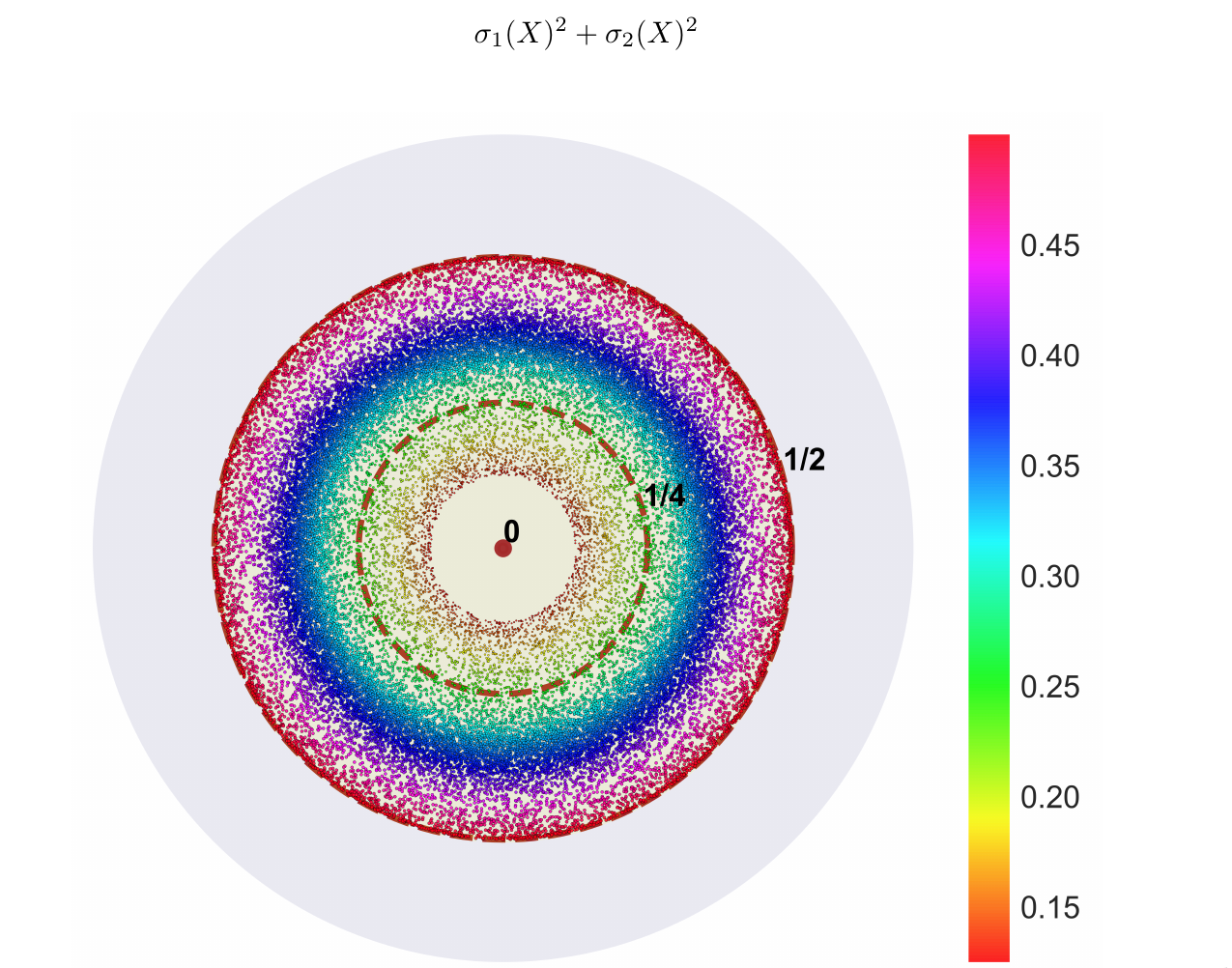
Refer to caption — Fig. 1: Numerical evidence of the validity of 4 where the samples $A,B$ are generated randomly (including normal and non-normal) with uniform distribution, and the distance from the origin (or colors) in the polar graph represents the value of $\sigma_{1}^{2}(X)+\sigma_{2}^{2}(X)$ .

Theorem 10.

Conjecture 5 holds when one of matrices $A,B\in\mathbb{C}^{d\times d}$ is normal and the other one is arbitrary.

It is obvious that our work leads to significant progress on Conjecture 5 (so, also Conjecture 4), as well as towards the distillability problem. If we relax the condition on the square sum of the norms of $A$ and $B$ , Theorem 10 reduces to the following result.

Corollary 11.

Let $A,B\in\mathbb{C}^{d\times d}(d\geqslant 4)$ , $\mathrm{Tr}(A)=\mathrm{Tr}(B)=0$ and one of $A$ and $B$ is normal and the other one is arbitrary. Denote

X=A\otimes\mathds{I}+\mathds{I}\otimes B,

(14)

and let $\sigma_{i}(X)$ be the $i$ -th largest singular value of $X$ . Then

\sigma_{1}^{2}(X)+\sigma_{2}^{2}(X)\leqslant\frac{3d-4}{d}\left(\left\lVert{A}\right\rVert_{F}^{2}+\left\lVert{B}\right\rVert_{F}^{2}\right).

(15)

Actually, the upper bound in Theorem 10 is attainable. For example, Let

A=\mathrm{diag}(2(d-1)\beta,-2\beta,\ldots,-2\beta),

(16)

and

B=\mathrm{diag}((d-2)\beta,(d-2)\beta,-2\beta,\ldots,-2\beta),

(17)

where

\beta=\left(d\sqrt{6d-8}\right)^{-1}.

(18)

Then $\mathrm{Tr}(A)=\mathrm{Tr}(B)=0$ , $\left\lVert{A}\right\rVert_{F}^{2}+\left\lVert{B}\right\rVert_{F}^{2}=\frac{1}{d}$ and

\sigma_{1}^{2}(X)+\sigma_{2}^{2}(X)=\frac{3d-4}{d^{2}}.

(19)

Hence, we have the following results.

Theorem 12.

Denote by $\bm{\mathcal{X}}^{(1)}_{d}$ the subset of $\bm{\mathcal{X}}$ where one of $A$ and $B$ is normal. Then

\max_{X\in\bm{\mathcal{X}}^{(1)}_{d}}\sigma_{1}^{2}(X)+\sigma_{2}^{2}(X)=\frac{3d-4}{d^{2}}.

(20)

Corollary 13.

Let $\bm{\mathcal{X}}^{(2)}_{d}$ be the set of matrices $A\otimes\mathds{I}+\mathds{I}\otimes B$ with $A,B$ traceless and one of $A$ and $B$ normal. Then

\max_{X\in\bm{\mathcal{X}}^{(2)}_{d}}\sigma_{1}^{2}(X)+\sigma_{2}^{2}(X)=\dfrac{3d-4}{d}\left(\left\lVert{A}\right\rVert_{F}^{2}+\left\lVert{B}\right\rVert_{F}^{2}\right).

(21)

The rest of the paper is organized as follows. In Section II, we will introduce some necessary mathematical notations and the background of optimization theory. In particular, we provide two useful lemmas which will be used in the proof of our main result repeatedly. In Section III, the proof of our main result is provided, that is, prove the validness of 5 when $A$ is normal. Finally, some concluding remarks are given in Section IV.

II Preliminaries

II-A Mathematical Notations

Let us first introduce some mathematical notations. We refer to $\mathbb{C}^{d\times d}$ , $\mathbb{R}^{d\times d}$ , and $\mathbb{H}^{d\times d}$ as the $d\times d$ complex matrices, real matrices, and Hermitian matrices, respectively.

To be clearly, hereafter in this paper, we use the capital letters to indicate the matrices, for example, $A\in\mathbb{C}^{d\times d}$ . On the other hand, we use the bold lowercase letters to indicate the vectors, for example, $\bm{a}\in\mathbb{C}^{d}$ . In particular, throughout this paper, we use $\bm{e}_{i},i=1,\ldots,d$ to indicate the natural basis in $\mathbb{C}^{d}(\text{ or }\mathbb{R}^{d})$ , that is, $\bm{e}_{i}$ is the vector whose $i$ -th entry is one and all the others are zeros.

By convention, $a_{i}$ is denoted as the $i$ -th entry of the vector $\bm{a}$ and $a_{ij}$ the $(i,j)$ -th entry of the matrix $A$ .

For any matrix $A=(a_{ij})\in\mathbb{C}^{d\times d}$ , we use $\left\lVert{A}\right\rVert_{F}$ to denote the Frobenius Norm :

\left\lVert{A}\right\rVert_{F}=\sqrt{\sum_{ij=1}^{d}|a_{ij}|^{2}}.

(22)

Another important operator for matrices is the trace operator :

\mathrm{Tr}(A)=\sum_{i=1}^{d}a_{ii}.

(23)

In addition, we have the relation:

\mathrm{Tr}(AA^{\dagger})=\mathrm{Tr}(A^{\dagger}A)=\left\lVert{A}\right\rVert_{F}^{2},

(24)

where $A^{\dagger}$ indicates the conjugate transpose of $A$ . Moreover, $A^{\intercal}$ indicates the transpose of the matrix $A$ . A matrix $A$ with $M$ rows and $N$ columns is called an $M\times N$ matrix, while $M$ and $N$ are called its dimensions. By convention, we use $\mathrm{dim}(A)$ to indicate the dimension if $A$ is square, i.e., $\mathrm{dim}(A)=N$ . Morevoer, we say a matric $A$ is traceless when $\mathrm{Tr}(A)=0$ .

For a vector $\bm{a}\in\mathbb{C}^{d}$ , we use $\left\lVert{\bm{a}}\right\rVert$ to denote the Euclidean norm, that is,

\left\lVert{\bm{a}}\right\rVert=\sqrt{\sum_{i=1}^{d}|a_{i}|^{2}}=\sqrt{\mathrm{Tr}(\bm{a}\bm{a}^{\dagger})}=\sqrt{\langle\bm{a},\bm{a}\rangle}.

(25)

Throughout this paper, we use $\mathds{I}$ to denote the identity operator. In particular, $\mathds{I}_{d}$ indicates the identity operator of order $d$ . If no other specified, the order of $\mathds{I}$ should match the operations in context.

Given two matrices $A=(a_{ij})$ and $B=(b_{ij})$ in $\mathbb{C}^{d\times d}$ , the tensor product (Kronecker product [39]) is defined as

A\otimes B=\begin{bmatrix}a_{11}B&\cdots&a_{1d}B\\ \vdots&\ddots&\vdots\\ a_{d1}B&\cdots&a_{dd}B\end{bmatrix}.

(26)

For any two Hilbert spaces $\mathcal{H}_{1}$ and $\mathcal{H}_{2}$ , the tensor space is defied by

\mathcal{H}_{1}\otimes\mathcal{H}_{2}=\{\lvert u\rangle\otimes\lvert v\rangle:\lvert u\rangle\in\mathcal{H}_{1},\lvert v\rangle\in\mathcal{H}_{2}\}.

(27)

In addition, the direct sum $A\oplus B$ is defined as

A\oplus B=\begin{bmatrix}A&0\\ 0&B\end{bmatrix}

(28)

for any two given square matrices.

For any matrix $A$ , denote by $\lambda_{i}(A)$ and $\sigma_{i}(A)$ the $i$ -th largest eigenvalue and singular value of $A$ , respectively. For any two matrices $X$ and $Y$ , we say $X$ is unitarily similar to $Y$ , i.e., $X\sim Y$ , when there exists a unitary operator $U$ such that $X=UYU^{\dagger}$ . In particular, in the composite system $\mathcal{H}_{1}\otimes\mathcal{H}_{2}$ , $X$ is said to be locally unitarily similar to $Y$ if there exist unitary operators $U$ and $V$ acting on $\mathcal{H}_{1}$ and $\mathcal{H}_{2}$ , respectively, such that $X=(U\otimes V)Y(U\otimes V)^{\dagger}$ , where $X$ and $Y$ are the operators acting on $\mathcal{H}_{1}\otimes\mathcal{H}_{2}$ .

Let $\mathcal{P}$ denotes the set of all matrices which is locally unitarily similar to

\oplus_{i=1}^{l}B_{i},

(29)

where each $B_{i}$ is either an $1\times 1$ or $2\times 2$ matrix and $\sum_{i=1}^{l}\mathrm{dim}(B_{i})=d$ .

As for the singular values, there exists a well-known Weyl’s inequality.

Lemma 14 (Weyl’s inequality [40]).

Let $A$ and $B$ are two matrices in $\mathbb{C}^{d\times d}$ . Then

\sigma_{i+j-1}(A+B)\leqslant\sigma_{i}(A)+\sigma_{j}(B),

(30)

for all $1\leqslant i,j\leqslant d,i+j\leqslant d$ . In particular,

\sigma_{1}(A+B)\leqslant\sigma_{1}(A)+\sigma_{1}(B).

(31)

II-B Supporting Lemmas in Optimization Theory

Our developments in the next section will be heavily relied on the optimization theory. Given a function $f$ , the maximization problem with linear and quadratic constraints can be formulated as:

\begin{array}[]{rl}\max&\quad f(\bm{x})\\ \text{s.t.}&\quad\begin{cases}\langle\bm{c}_{i},\bm{x}\rangle&=0,\quad i=1,\ldots,m,\\ \bm{x}^{\dagger}W\bm{x}&=r,\end{cases}\end{array}

(32)

where $\bm{c}_{i}\in\mathbb{R}^{N},\;\bm{x}\in\mathbb{R}^{N}$ , $W\in\mathbb{R}^{N\times N}$ , and $r\in\mathbb{R}$ . Here $f$ is usually called the objective function which is desired to be maximized.

In particular, the quadratic constraints in this paper always appear as the following form:

\sum_{i=1}^{N}w_{i}x_{i}^{2}=r,\quad w_{i}>0,\quad r>0.

(33)

That is, $W$ is a positive diagonal matrix. Moreover, the objective function $f$ is always continuous differentiable and degree- $2$ homogeneous. Recall that, a function $f(\bm{x})$ with $\bm{x}\in\mathbb{R}^{N}$ is degree- $k$ homogeneous $(k>0)$ if

f(t\bm{x})=t^{k}f(\bm{x}),\quad\forall\;t\in\mathbb{R}.

(34)

In addition, we say that a vector $\bm{x}$ is a feasible point of the optimization problem (32) if it satisfies all the constraints of the optimization problem, i.e., the linear and quadratic constraints in (32).

The set $\mathcal{S}$ is said to be feasible set of the optimization problem if it is the set of all feasible points. In particular, the optimal solution of the optimization problem is the one at which the objective function achieves its maximal value.

One should be noted that for a specific optimization problem, there may exist many different optimal solutions. Moreover, the optimization problem (32) can be written in the following form:

\max_{\bm{x}\in\mathcal{S}}f(\bm{x}).

(35)

Denote by $\mathcal{L}$ the Lagrange function

\mathcal{L}(\bm{x},\bm{\mu},\nu)=f(\bm{x})-\sum_{i=1}^{m}\mu_{i}\langle\bm{c}_{i},\bm{x}\rangle-\nu(\bm{x}^{\dagger}W\bm{x}-r),

(36)

where $\bm{\mu}=(\mu_{1},\mu_{2},\ldots,\mu_{m})^{\intercal}\in\mathbb{R}^{m}$ and $\nu\in\mathbb{R}$ . Then we have the well-known KKT condition for the optimization problem.

Lemma 15 (First order KKT condition [41]).

Suppose the optimization problem is defined by (32) with Lagrange function defined by (36). If $\bm{x}^{*}$ is a optimized solution to the problem, then there exist $\mu_{i}^{*}\in\mathbb{R}$ and $\nu^{*}\in\mathbb{R}$ such that

\left.\nabla\mathcal{L}(\bm{x},\bm{\mu},\nu)\right|_{(\bm{x}^{*},\bm{\mu}^{*},\nu^{*})}=0,

(37)

that is,


$\displaystyle\nabla f(\bm{x}^{})-\sum_{i=1}^{m}\mu_{i}^{}\bm{c}_{i}-2\nu^{}W\bm{x}^{}$	$\displaystyle=0,$	(38a)
$\displaystyle\langle\bm{c}_{i},\bm{x}^{*}\rangle$	$\displaystyle=0,$	(38b)
$\displaystyle\langle\bm{x}^{},W\bm{x}^{}\rangle$	$\displaystyle=r.$	(38c)

The following two lemmas about the necessary conditions of the optimization problem are useful.

Lemma 16.

Suppose $f(\bm{x})$ is a degree-two homogeneous function where $\bm{x}\in\mathbb{R}^{N}$ . The optimization problem is defined as follows:

\begin{array}[]{rl}\max&\quad f(\bm{x})+\sum_{i=1}^{M}\xi_{i}y_{i}^{2}\\ \mathrm{s.t.}&\quad\begin{cases}\langle\bm{c}_{i},\bm{x}\rangle&=0,\\ \sum_{i=1}^{N}\tau_{i}~x_{i}^{2}+\sum_{i=1}^{M}\omega_{i}y_{i}^{2}&=r,\end{cases}\end{array}

(39)

where $\bm{y}\in\mathbb{R}^{M}$ , $\bm{c_{i}}\in\mathbb{R}^{N},\;i=1,\ldots,m,$ , $\xi_{i}\in\mathbb{R}$ , $\tau_{i}~>0$ , and $\omega_{i}>0$ . Denote by $\mathcal{S}$ the feasible set of the optimization problem. Let $(\bm{x}^{*},\bm{y}^{*})$ be an optimal solution. Then

\max_{(\bm{x},\bm{y})\in\mathcal{S}}f(\bm{x})+\sum_{i=1}^{M}\xi_{i}y_{i}^{2}=\eta r,\quad\text{or}\quad\bm{y}^{*}=0.

(40)

where $\eta=\max\{\frac{\xi_{i}}{\omega_{i}},i=1,2,\ldots,M\}$ .

Lemma 17.

Suppose the optimization problem is defined as follows:

\begin{array}[]{rl}\max&\quad f(\bm{x})\\ \text{s.t.}&\quad\begin{cases}\langle\bm{c},\bm{x}\rangle+\sum_{i=1}^{M}y_{i}&=0,\\ \langle\bm{d}_{i},\bm{x}\rangle&=0,\\ \sum_{i=1}^{N}\tau_{i}~x_{i}^{2}+\sum_{i=1}^{M}y_{i}^{2}&=r,\end{cases}\end{array}

(41)

where $\bm{x},\;\bm{c}\in\mathbb{R}^{N},\;\bm{d}_{i}\in\mathbb{R}^{N},\;i=1,\ldots,m,,\;\bm{y}\in\mathbb{R}^{M}$ and $\tau_{i}>0$ . In addition, $f$ is degree-2 homogeneous and $f(\bm{x}^{0})>0$ for some feasible point $\bm{x}^{0}$ . Then, the maximal value of the objective function $f$ is achieved only when

y_{1}=y_{2}=\cdots=y_{M}.

(42)

For the sake of conciseness, we move the proofs of the above lemmas to Appendices A and B, respectively.

III Proof of the Main Result

In this section, we will prove our main result Theorem 10, that is, the validity of 5 when one of $A$ and $B$ is normal and the other is arbitrary. With a locally unitary similarity, we can assume that $A$ is diagonal. Therefore, in the following development of this section we always assume that

A=\mathrm{diag}(a_{1},a_{2},\ldots,a_{d})\in\mathbb{C}^{d\times d}.

(43)

Thus, $X$ can be written as a direct sum

X=\oplus_{i=1}^{d}(a_{i}\mathds{I}+B).

(44)

In order to prove Theorem 10, we prove the following theorem first, which can be regarded as the real version of Theorem 10.

Theorem 18.

Conjecture 5 holds when

A=\mathrm{diag}(a_{1},a_{2},\ldots,a_{d})\in\mathbb{R}^{d\times d},\quad\quad B\in\mathbb{R}^{d\times d}.

(45)

Note that the set of singular values of $X$ consists of all the singular values of each block $a_{i}\mathds{I}+B$ . Then the problem of proving Theorem 18 naturally split into two different cases:

Case 1

: the largest two singular values of $X$ come from the same block, say $a_{1}\mathds{I}+B$ ;
Case 2

: the largest two singular values of $X$ come from two different blocks, say $a_{1}\mathds{I}+B$ and $a_{2}\mathds{I}+B$ .

In the following we discuss these two cases separately.

III-A Case 1: the Largest Two Singular Values of $X$ Come From the Same Block

We have the following result for this case.

Lemma 19.

Let $X=A\otimes\mathds{I}+\mathds{I}\otimes B\in\bm{\mathcal{X}}_{d}\,(d\geqslant 4)$ with $A=\mathrm{diag}(a_{1},a_{2},\ldots,a_{d})$ . If

\sigma_{1}(X)=\sigma_{1}(a_{1}\mathds{I}+B),\quad\quad\sigma_{2}(X)=\sigma_{2}(a_{1}\mathds{I}+B),

(46)

then

\sigma_{1}^{2}(X)+\sigma_{2}^{2}(X)\leqslant\frac{3d-4}{d^{2}}.

(47)

Proof.

Denote by $B=(b_{ij})_{i,j=1}^{d}$ . Note that


$\displaystyle\sigma_{i}^{2}(X)$	$\displaystyle=\sigma_{i}^{2}(a_{1}\mathds{I}+B)=\lambda_{i}(a_{1}^{2}\mathds{I}+a_{1}(B+B^{\intercal})+BB^{\intercal})$	(48a)
	$\displaystyle=a_{1}^{2}+\lambda_{i}(a_{1}(B+B^{\intercal})+BB^{\intercal}),\quad i=1,2.$	(48b)

Denote by $\bm{\phi}$ and $\bm{\psi}$ the two unit eigenvectors (up to a phase multiplication) associated with the first and second largest eigenvalues of $a_{1}(B+B^{\intercal})+BB^{\intercal}$ , respectively. With an orthogonal similarity, we can assume that $\bm{\phi}=\bm{e}_{1}$ and $\bm{\psi}=\bm{e}_{2}$ , i.e., replace $B$ with $UBU^{\intercal}$ by some orthogonal operator $U$ . Hence,

$\displaystyle\sigma_{1}^{2}(X)+\sigma_{2}^{2}(X)$	$\displaystyle=2a_{1}^{2}+\mathrm{Tr}((a_{1}(B+B^{\intercal})+BB^{\intercal})(\bm{\phi}\bm{\phi}^{\dagger}+\bm{\psi}\bm{\psi}^{\dagger}))$	(49)
	$\displaystyle=2a_{1}^{2}+2a_{1}(b_{11}+b_{22})+\sum_{i=1}^{d}(b_{1i}^{2}+b_{2i}^{2})$	(50)
	$\displaystyle=(a_{1}+b_{11})^{2}+(a_{1}+b_{22})^{2}+\sum^{2}_{i=1}\sum_{j\neq i}b_{ij}^{2}.$	(51)

Consider $A$ and $\mathrm{diag}(B)$ , they are both normal and traceless, by Corollary 9, we have

(a_{1}+b_{11})^{2}+(a_{1}+b_{22})^{2}\leqslant\frac{3d-4}{d}\sum_{i=1}^{d}(a_{i}^{2}+b_{ii}^{2}).

(52)

Therefore, by (51), we have


$\displaystyle\sigma_{1}^{2}(X)+\sigma_{2}^{2}(X)$	$\displaystyle\leqslant\frac{3d-4}{d}\sum_{i=1}^{d}(a_{i}^{2}+b_{ii}^{2})+\sum^{2}_{i=1}\sum_{j\neq i}b_{ij}^{2}$	(53a)
	$\displaystyle=\frac{3d-4}{d}(\frac{1}{d}-\sum_{i\neq j}b_{ij}^{2})+\sum^{2}_{i=1}\sum_{j\neq i}b_{ij}^{2}$	(53b)
	$\displaystyle\leqslant\frac{3d-4}{d^{2}}-\frac{2d-4}{d}\sum_{i\neq j}b_{ij}^{2}$	(53c)
	$\displaystyle\leqslant\frac{3d-4}{d^{2}},$	(53d)

which completes our proof. ∎

III-B Case 2: the Largest Two Singular Values of $X$ Come From Two Different Blocks

We shall consider the case when $B\in\mathcal{P}$ first, where $B$ is the direct sum of blocks of at most dimension two. After that, we can extend this result to the general $B$ .

Recall that if $B\in\mathcal{P}$ , then $B$ is the direct sum of several square matrices, i.e.,

B=\oplus_{i=1}^{l}B_{i},\quad\mathrm{dim}(B_{i})\leqslant 2,\quad\sum_{i=1}^{l}\mathrm{dim}(B_{i})=d.

(54)

Lemma 20.

Suppose $X=A\otimes\mathds{I}+\mathds{I}\otimes B$ with $A,B\in\mathbb{R}^{d\times d}\;(d\geqslant 4)$ , $\mathrm{Tr}(A)=\mathrm{Tr}(B)=0$ , $\left\lVert{A}\right\rVert_{F}^{2}+\left\lVert{B}\right\rVert_{F}^{2}=\frac{1}{d}$ , $A=\mathrm{diag}(a_{1},a_{2},\ldots,a_{d})$ and $B\in\mathcal{P}$ . If the largest two singular values of $X$ come from two different blocks, i.e.,

\sigma_{1}(X)=\sigma_{1}(a_{1}\mathds{I}+B),\quad\quad\sigma_{2}(X)=\sigma_{1}(a_{2}\mathds{I}+B),

(55)

then

\sigma_{1}^{2}(X)+\sigma_{2}^{2}(X)\leqslant\frac{3d-4}{d^{2}}.

(56)

Proof.

Lemma 20 is proved in Appendix C. ∎

Now we extend Lemma 20 to general $B$ .

Lemma 21.

Suppose $X=A\otimes\mathds{I}+\mathds{I}\otimes B$ with $A,B\in\mathbb{R}^{d\times d}\;(d\geqslant 4)$ , $\mathrm{Tr}(A)=\mathrm{Tr}(B)=0$ , $\left\lVert{A}\right\rVert_{F}^{2}+\left\lVert{B}\right\rVert_{F}^{2}=\frac{1}{d}$ , and $A=\mathrm{diag}(a_{1},a_{2},\ldots,a_{d})$ . If the largest two singular values of $X$ come from two different blocks, i.e.,

\sigma_{1}(X)=\sigma_{1}(a_{1}\mathds{I}+B)\text{ and }\sigma_{2}(X)=\sigma_{1}(a_{2}\mathds{I}+B),

(57)

then

\sigma_{1}^{2}(X)+\sigma_{2}^{2}(X)\leqslant\frac{3d-4}{d^{2}}.

(58)

Proof.

Let


	$\displaystyle Y_{i}$	$\displaystyle=(a_{i}\mathds{I}+B)(a_{i}\mathds{I}+B)^{\intercal}=a_{i}^{2}\mathds{I}+a_{i}(B+B^{\intercal})+BB^{\intercal},\quad i=1,2.$		(59a)

Then $\sigma_{1}^{2}(X)=\lambda_{1}(Y_{1})$ and $\sigma_{2}^{2}(X)=\lambda_{1}(Y_{2})$ . Suppose $\bm{\phi}$ and $\bm{\psi}$ are the unit eigenvectors associated with the largest eigenvalues of $Y_{1}$ and $Y_{2}$ , respectively. With an orthogonal similarity of $B$ , i.e., replace $B$ with $UBU^{\intercal}$ by some orthogonal operator $U$ , we can assume that

\bm{\phi}=\bm{e}_{1},\quad\bm{\psi}=\cos\theta\bm{e}_{1}+\sin\theta\bm{e}_{2},\quad\theta\in[0,2\pi].

(60)

Furthermore, applying an orthogonal similarity on $B$ with the first two dimensions kept the same, we can further assume

b_{1j}=0,\;j\geqslant 4,\quad\text{and}\quad b_{2j}=0,\;j\geqslant 5.

(61)

Let $h=\sigma_{1}^{2}(X)+\sigma_{2}^{2}(X)$ . Then,

\displaystyle h

\displaystyle=\lambda_{1}(Y_{1})+\lambda_{1}(Y_{2})=\bm{\phi}^{\dagger}Y_{1}\bm{\phi}+\bm{\psi}^{\dagger}Y_{2}\bm{\psi}=h_{1}+h_{2}+b_{24}^{2}\sin^{2}\theta,

(62)

where

h_{1}=\sin(2\theta)\left(a_{2}(b_{12}+b_{21})+b_{11}{b}_{21}+b_{12}{b}_{22}\right)+(1+\cos^{2}\theta)b_{12}^{2}\\ +\cos^{2}\theta(a_{2}+b_{11})^{2}+(a_{1}+b_{11})^{2}+\sin^{2}\theta((a_{2}+b_{22})^{2}+b_{21}^{2}),

(63)

and

h_{2}=b_{13}^{2}+(\cos\theta b_{13}+\sin\theta b_{23})^{2}.

(64)

Let

\mathcal{B}=\{b_{ij}:i\neq j\&\;(i,j)\not\in\{(1,2),(2,1),(1,3),(2,3),(2,4)\}\},

(65)

be the set where the parameters are not involved in the objective function $h$ and the related linear constraints. Hence, we can replace $b_{ij}\in\mathcal{B}$ by $0$ ’s and multiply a scalar (denoted as $\beta$ ) to all the rest variables simultaneously in order to satisfy the related quadratic constraint. It is easy to see that $\beta>1$ if some of $b_{ij}\in\mathcal{B}$ are nonzero. In this way, the linear constraints are also satisfied and the value of function $h$ is replaced by

\beta^{2}h>h,

(66)

since $\beta>1$ and $h$ is a positive degree- $2$ homogeneous function. We now find another feasible point such that $h$ achieves a greater value. Hence, it suffices to assume

b_{ij}=0,\quad\forall i\neq j\in\mathcal{B}.

(67)

Note that to find the maximal value of $h$ is equivalent to solve the following optimization problem:

\begin{array}[]{rl}\max&\quad h\\ \text{ s.t. }&\begin{cases}\sum\limits_{i=1}^{d}a_{i}=0,\\ \sum\limits_{i=1}^{d}b_{i}=0,\\ \sum\limits_{i=1}^{d}\!a_{i}^{2}+\sum\limits_{i,j\not\in\mathcal{B}}b_{ij}^{2}=\frac{1}{d}.\end{cases}\end{array}

(68)

Let

b_{13}=t\cos\alpha,\quad b_{23}=t\sin\alpha,\quad\alpha\in[0,2\pi].

(69)

Then

h_{2}=t^{2}(\cos^{2}\alpha+\cos^{2}(\alpha-\theta)).

(70)

Therefore, the original optimization problem (68) is reduced to the following one:

\begin{array}[]{rl}\max&\quad f(\bm{x})+\xi_{1}y_{1}^{2}+\xi_{2}y_{2}^{2}\\ \text{s.t.}&\quad\begin{cases}\langle\bm{c_{i}},\bm{x}\rangle&=0,\\ \sum_{i=1}^{2d+2}\tau_{i}~|x_{i}|^{2}+\omega_{1}y_{1}^{2}+\omega_{2}y_{2}^{2}&=r,\end{cases}\end{array}

(71)

where

$\displaystyle\bm{x}$	$\displaystyle=(a_{1},a_{2},\ldots,a_{d},b_{11},b_{22},\ldots,b_{dd},b_{12},b_{21})^{\intercal},$	(72)
$\displaystyle\bm{c}_{1}$	$\displaystyle=(\underbrace{1,1,\ldots,1}_{d\text{ times}},0,0,\ldots,0,0,0)^{\intercal}\in\mathbb{R}^{2d+2},$
$\displaystyle\bm{c}_{2}$	$\displaystyle=(0,0,\ldots,0,\underbrace{1,1,\ldots,1}_{d\text{ times}},0,0)^{\intercal}\in\mathbb{R}^{2d+2},$

and

\displaystyle\bm{y}=(b_{24},t)^{\intercal},\quad\tau_{i}=\omega_{i}=1,\quad\xi_{1}=\sin^{2}\theta,\quad\xi_{2}=\cos^{2}\alpha+\cos^{2}(\alpha-\theta),\quad r=\frac{1}{d}.

(73)

In particular,

f(\bm{x})=(x_{1}+x_{d+1})^{2}+\cos^{2}\theta(x_{2}+x_{d+1})^{2}+\sin^{2}\theta((x_{2}+x_{d+2})^{2}+x_{2d+2}^{2})\\ +(1+\cos^{2}\theta)x_{2d+1}^{2}+\sin(2\theta)\left(x_{d+1}{x}_{2d+2}+x_{2d+1}{x}_{d+2}+x_{2}(x_{2d+1}+x_{2d+2})\right).

(74)

Let

\eta=\max\{\frac{\xi_{i}}{\omega_{i}},i=1,2\}.

(75)

It is eay to see that

\eta=\max\{\sin^{2}\theta,\cos^{2}\alpha+\cos^{2}(\alpha-\theta)\}\leqslant 2.

(76)

Note that $f(\bm{x})$ is degree- $2$ homogeneous. Therefore, according to Lemma 16, we have either

\displaystyle\max\sigma_{1}^{2}(X)+\sigma_{2}^{2}(X)

\displaystyle=\max(h_{1}+h_{2}+b_{24}^{2}\sin^{2}\theta)=\frac{\eta}{d}\leqslant\frac{2}{d}\leqslant\frac{3d-4}{d^{2}},

(77)

or $\sigma_{1}^{2}(X)+\sigma_{2}^{2}(X)$ achieves the maximal value only when $\bm{y}=0$ , i.e., $b_{13}=b_{23}=b_{24}=0$ .

For the latter case, the matrix $B$ has the shape as follows:

B=\begin{bmatrix}b_{11}&b_{12}\\ b_{21}&b_{22}\\ \end{bmatrix}\oplus\mathrm{diag}(b_{33},b_{44},\ldots,b_{dd}),

(78)

and then $B\in\mathcal{P}$ . Hence, Lemma 21 follows directly from Lemma 20. ∎

Theorem 18 can be proved based on Lemmas 19 and 21 as follows.

Proof of Theorem 18.

$X$ is a direct sum of $d$ blocks. Then, the set of singular values of $X$ consists of all the singular values of all the different blocks. By Lemma 19, the inequality (9) holds when the largest two singular values of $X$ come from a single block. On the other hand, by Lemma 21, the inequality (9) also holds when the largest two singular values of $X$ come from two different blocks. Hence Theorem 18 follows. ∎

We are now ready to prove Theorem 10.

Proof of Theorem 10.

Since $A=\mathrm{diag}(a_{1},a_{2},\ldots,a_{d})$ and thus

X=\oplus_{i=1}^{d}(a_{i}\mathds{I}+B).

(79)

Let $Y=XX^{\dagger}$ . Then

Y=\oplus_{i=1}^{d}\left[(a_{i}\mathds{I}+B)(a_{i}\mathds{I}+B)^{\dagger}\right].

(80)

Suppose $\bm{\phi}_{i}$ are the two unit eigenvectors of $Y$ corresponding to its largest two eigenvalues. Note that $Y$ is the direct sum of $d$ block matrices, its eigenvalues consist of all the eigenvalues of every block. Moreover, the eigenvectors of $Y$ have the shapes:

\bm{\phi}_{i}=\bm{e}_{i}\otimes\bm{y}_{i},\quad\bm{e}_{i},\bm{y}_{i}\in\mathbb{C}^{d},\;i=1,\ldots,d^{2},\;

(81)

where $\bm{e}_{i},i=1,\ldots,d$ is the natural basis in $\mathbb{C}^{d}$ . In particular, we will have the two different cases up to an index permutation:

(i)

$\bm{\phi}_{1}=\bm{e}_{1}\otimes\bm{y}_{1}$ and $\bm{\phi}_{2}=\bm{e}_{1}\otimes\bm{y}_{2}$ ;
(ii)

$\bm{\phi}_{1}=\bm{e}_{1}\otimes\bm{y}_{1}$ and $\bm{\phi}_{2}=\bm{e}_{2}\otimes\bm{y}_{2}$ .

In case (i): we have $\langle\bm{y}_{1},\bm{y}_{2}\rangle=0$ . Hence, there exists a unitary operator $U$ such that

U(\bm{y}_{1},\bm{y}_{2})=(\bm{e}_{1},\bm{e}_{2}).

(82)

In case (ii): we can find a unitary operator $U_{1}$ such that

U_{1}(\bm{y}_{1},\bm{y}_{2})=(\bm{e}_{1},c_{1}\bm{e}_{1}+c_{2}\bm{e}_{2}),

(83)

where $c_{1},c_{2}\in\mathbb{C}$ . Suppose

\displaystyle c_{1}

\displaystyle=r_{1}e^{\mathrm{i}\mkern 1.0mu\theta_{1}},\quad\quad c_{2}=r_{2}e^{\mathrm{i}\mkern 1.0mu\theta_{2}},\quad\theta_{1},\theta_{2}\in[0,2\pi],\quad r_{1}^{2}+r_{2}^{2}=1,

(84)

and let

U_{2}=\mathrm{diag}(1,e^{\mathrm{i}\mkern 1.0mu(\theta_{1}-\theta_{2})},1,\ldots,1)\in\mathbb{C}^{d\times d}.

(85)

Then

U(\bm{y}_{1},\bm{y}_{2})=(\bm{e}_{1},e^{\mathrm{i}\mkern 1.0mu\theta_{1}}(r_{1}\bm{e}_{1}+r_{2}\bm{e}_{2})),

(86)

where $U=U_{2}U_{1}$ . Note that if $\bm{x}$ is an eigenvector of a Hermitian matrix, then $e^{\mathrm{i}\mkern 1.0mu\theta}\bm{x}$ is also the eigenvector corresponding to the same eigenvalue. So, if we replace $B$ by $UBU^{\dagger}$ , then $\bm{e}_{1}$ and $r_{1}\bm{e}_{1}+r_{2}\bm{e}_{2}$ are the two eigenvectors of $Y$ associated with its largest two eigenvalues and these two eigenvectors are real.

Therefore, we can denote by $\bm{\phi}_{i}\in\mathbb{R}^{d^{2}}(i=1,2)$ the unit eigenvectors of $Y$ associated with its largest two eigenvalues, which are real. Then

\langle\bm{\phi}_{1},\bm{\phi}_{2}\rangle=0.

(87)

Let $X=X_{1}+\mathrm{i}\mkern 1.0muX_{2}$ with $X_{1},X_{2}\in\mathbb{R}^{d^{2}\times d^{2}}$ . Then,

Y=X_{1}X_{1}^{\intercal}+X_{2}X_{2}^{\intercal}+\mathrm{i}\mkern 1.0mu(X_{2}X_{1}^{\intercal}-X_{1}X_{2}^{\intercal}).

(88)

There

\displaystyle\sigma_{i}^{2}(X)

\displaystyle=\bm{\phi}^{\intercal}_{i}Y\bm{\phi}_{i}=\bm{\phi}^{\intercal}_{i}\left(X_{1}X_{1}^{\intercal}+X_{2}X_{2}^{\intercal}\right)\bm{\phi}_{i}+\mathrm{i}\mkern 1.0mu\left(\bm{\phi}^{\intercal}_{i}(X_{2}X_{1}^{\intercal}-X_{1}X_{2}^{\intercal})\bm{\phi}_{i}\right).

(89)

Since $\sigma_{i}^{2}(X)\geqslant 0$ , $\bm{\phi}_{i}\in\mathbb{R}^{d^{2}}$ , and $X_{1},X_{2}\in\mathbb{R}^{d^{2}\times d^{2}}$ , we have

\displaystyle\sigma_{i}^{2}(X)

\displaystyle=\bm{\phi}^{\intercal}_{i}\left(X_{1}X_{1}^{\intercal}+X_{2}X_{2}^{\intercal}\right)\bm{\phi}_{i}=\bm{\phi}^{\intercal}_{i}X_{1}X_{1}^{\intercal}\bm{\phi}_{i}+\bm{\phi}^{\intercal}_{i}X_{2}X_{2}^{\intercal}\bm{\phi}_{i}.

(90)

Moreover,

\displaystyle\max_{\stackrel{{\scriptstyle\langle\bm{\psi}_{1},\bm{\psi}_{2}\rangle=0}}{{\left\lVert{\psi_{1}}\right\rVert=\left\lVert{\psi_{2}}\right\rVert=1}}}\quad

\displaystyle\sum_{i=1}^{2}\bm{\psi}^{\intercal}_{i}X_{i}X_{i}^{\intercal}\bm{\psi}_{i}=\lambda_{1}(X_{i}X_{i}^{\intercal})+\lambda_{2}(X_{i}X_{i}^{\intercal})=\sigma_{1}^{2}(X_{i})+\sigma_{2}^{2}(X_{i}).

(91)

Thus, we have

\displaystyle\sigma_{1}^{2}(X)+\sigma_{2}^{2}(X)\leqslant\sigma_{1}^{2}(X_{1})+\sigma_{2}^{2}(X_{1})+\sigma_{1}^{2}(X_{2})+\sigma_{2}^{2}(X_{2}).

(92)

Note that

X_{1}=\mathrm{Re}(X)=\mathrm{Re}(A)\otimes\mathds{I}+\mathds{I}\otimes\mathrm{Re}(B),

(93)

which also satisfies the conditions:

$\displaystyle\mathrm{Tr}(\mathrm{Re}(A))$	$\displaystyle=\mathrm{Tr}(\mathrm{Re}(B))=0,$	(94)
$\displaystyle\mathrm{Re}(A)$	$\displaystyle=\mathrm{Re}(\mathrm{diag}(a_{1},a_{2},\ldots,a_{d}))\in\mathbb{R}^{d\times d},$	(95)
$\displaystyle\mathrm{Re}(B)$	$\displaystyle\in\mathbb{R}^{d\times d}.$	(96)

Let

s_{1}=[d(\left\lVert{\mathrm{Re}(A)}\right\rVert_{F}^{2}+\left\lVert{\mathrm{Re}(B)}\right\rVert_{F}^{2})]^{-1/2}.

(97)

Then we have by Theorem 18

\sigma_{1}^{2}(s_{1}X_{1})+\sigma_{2}^{2}(s_{1}X_{1})\leqslant\frac{3d-4}{d^{2}},

(98)

which gives

\sigma_{1}^{2}(X_{1})+\sigma_{2}^{2}(X_{1})\leqslant\frac{3d-4}{d}(\left\lVert{\mathrm{Re}(A)}\right\rVert_{F}^{2}+\left\lVert{\mathrm{Re}(B)}\right\rVert_{F}^{2}).

(99)

Similarly,

X_{2}=\mathrm{Im}(X)=\mathrm{Im}(A)\otimes\mathds{I}+\mathds{I}\otimes\mathrm{Im}(B),

(100)

which also satisfies the conditions:

$\displaystyle\mathrm{Tr}(\mathrm{Im}(A))$	$\displaystyle=\mathrm{Tr}(\mathrm{Im}(B))=0,$	(101)
$\displaystyle\mathrm{Im}(A)$	$\displaystyle=\mathrm{Im}(\mathrm{diag}(a_{1},a_{2},\ldots,a_{d}))\in\mathbb{R}^{d\times d},$	(102)
$\displaystyle\mathrm{Im}(B)$	$\displaystyle\in\mathbb{R}^{d\times d}.$	(103)

Let

s_{2}=[d(\left\lVert{\mathrm{Im}(A)}\right\rVert_{F}^{2}+\left\lVert{\mathrm{Im}(B)}\right\rVert_{F}^{2})]^{-1/2}.

(104)

Then we have by Theorem 18

\sigma_{1}^{2}(s_{2}X_{2})+\sigma_{2}^{2}(s_{2}X_{2})\leqslant\frac{3d-4}{d^{2}},

(105)

which gives

\sigma_{1}^{2}(X_{2})+\sigma_{2}^{2}(X_{2})\leqslant\frac{3d-4}{d}(\left\lVert{\mathrm{Im}(A)}\right\rVert_{F}^{2}+\left\lVert{\mathrm{Im}(B)}\right\rVert_{F}^{2}).

(106)

Therefore, by (92), we have

$\displaystyle\sigma_{1}^{2}(X)+\sigma_{2}^{2}(X)$	$\displaystyle\leqslant\frac{3d-4}{d}(\left\lVert{\mathrm{Re}(A)}\right\rVert_{F}^{2}+\left\lVert{\mathrm{Re}(B)}\right\rVert_{F}^{2})+\frac{3d-4}{d}(\left\lVert{\mathrm{Im}(A)}\right\rVert_{F}^{2}+\left\lVert{\mathrm{Im}(B)}\right\rVert_{F}^{2})$	(107)
	$\displaystyle=\frac{3d-4}{d}(\left\lVert{\mathrm{Re}(A)}\right\rVert_{F}^{2}+\left\lVert{\mathrm{Re}(B)}\right\rVert_{F}^{2}+\left\lVert{\mathrm{Im}(A)}\right\rVert_{F}^{2}+\left\lVert{\mathrm{Im}(B)}\right\rVert_{F}^{2})$	(108)
	$\displaystyle=\frac{3d-4}{d}(\left\lVert{A}\right\rVert_{F}^{2}+\left\lVert{B}\right\rVert_{F}^{2})$	(109)
	$\displaystyle=\frac{3d-4}{d^{2}},$	(110)

i.e., (9) holds. ∎

IV Conclusion

We have studied Conjecture 5 related to the entanglement distillability problem, one of the fundamental problems in quantum information theory. In Refs. [21, 38], this conjecture is answered partially when $A,B$ are both normal. In our main result–Theorem 10, we solved this open problem when one of $A$ and $B$ is normal and the other one is arbitrary utilizing the techniques of matrix analysis and optimization theory. Our Results-Theorems 10 and 12 and Corollaries 18 and 13 make significant progress on Conjecture 4 and 5, namely the two-undistillability of the one-copy undistillability NPT state.

Appendix A Proof of Lemma 16

Before proving Lemma 16, the following result is needed.

Lemma 22.

Suppose

$\displaystyle\bm{a}$	$\displaystyle=(a_{1},a_{2},\ldots,a_{N})^{\intercal},$	(111)
$\displaystyle\bm{b}$	$\displaystyle=(\,b_{1},b_{2},\ldots,\,b_{N})^{\intercal},$	(112)
$\displaystyle\bm{x}$	$\displaystyle=(x_{1},x_{2},\ldots,x_{N})^{\intercal},$	(113)

where $a_{i},x_{i}\in\mathbb{R}$ and $b_{i}>0$ . Then for any nonzero $\bm{x}\in\mathbb{R}^{N}$ ,

\displaystyle\frac{\sum_{i=1}^{N}a_{i}x_{i}^{2}}{\sum_{i=1}^{N}b_{i}x_{i}^{2}}\leqslant\max\left\{\frac{a_{i}}{b_{i}},\;i=1,2,\ldots,N\right\}.

(114)

Proof.

Denote by $\bm{c}=(\sqrt{b_{1}},\sqrt{b_{2}},\ldots,\sqrt{b_{N}})^{\intercal}$ , $A=\mathrm{diag}(\bm{a})$ , $B=\mathrm{diag}(\bm{b})$ , and $C=\mathrm{diag}(\bm{c})$ . Then $B=C^{2}$ and

$\displaystyle\frac{\sum_{i=1}^{N}a_{i}x_{i}^{2}}{\sum_{i=1}^{N}b_{i}x_{i}^{2}}$	$\displaystyle=\frac{\langle\bm{x},A\bm{x}\rangle}{\langle\bm{x},B\bm{x}\rangle}=\frac{\langle\bm{x},A\bm{x}\rangle}{\langle\bm{x},C^{2}\bm{x}\rangle}=\frac{\langle C\bm{x},(C^{-1}AC^{-1})C\bm{x}\rangle}{\langle C\bm{x},C\bm{x}\rangle}$	(115)
	$\displaystyle=\frac{\langle\bm{y},(C^{-1}AC^{-1})\bm{y}\rangle}{\langle\bm{y},\bm{y}\rangle}$	(116)
	$\displaystyle\leqslant\lambda_{1}(C^{-1}AC^{-1})$	(117)
	$\displaystyle=\lambda_{1}(AB^{-1})$	(118)
	$\displaystyle=\max\left\{\frac{a_{i}}{b_{i}},\;i=1,2,\ldots,N\right\},$	(119)

where $\bm{y}=C\bm{x}$ . ∎

Proof of Lemma 16.

Suppose $f(\bm{x})+\sum_{i=1}^{M}\xi_{i}y_{i}^{2}$ achieves its maximal value at $(\bm{x}^{*},\bm{y}^{*})$ . Let

\zeta=f(\bm{x}^{*})+\sum_{i=1}^{M}\xi_{i}|y_{i}^{*}|^{2}=\max_{(\bm{x},\bm{y})\in\mathcal{S}}f(\bm{x})+\sum_{i=1}^{M}\xi_{i}y_{i}^{2}.

(120)

Without the loss of generality, we can assume $\eta=\frac{\xi_{1}}{w_{1}}$ . Then we must have

\zeta\geqslant\eta r,

(121)

since the value $\eta r$ can be achieved at $\bm{x}=0,\;y_{1}=\frac{\sqrt{r}}{\sqrt{w_{1}}}$ and $y_{i}=0,\;i\geqslant 2$ .

We prove this lemma by contradiction.

Assume that result of Lemma 16, i.e., (40) does not hold:

\bm{y}^{*}\neq 0\text{ and }\zeta>\eta r.

(122)

Let

\displaystyle r_{1}

\displaystyle=\sum_{i=1}^{N}\tau_{i}|x_{i}^{*}|^{2},\quad\text{and}\quad r_{2}=\sum_{i=1}^{M}\omega_{i}|y_{i}^{*}|^{2}.

(123)

By the quadratic constraint of the optimization problem (39), we must have

r_{1}+r_{2}=r,\quad r_{1}\geqslant 0,\;r_{2}>0.

(124)

If $r_{1}=0$ , then $\bm{x}=0$ . Let $u_{i}=\sqrt{w_{i}}|y_{i}^{*}|$ , then

\displaystyle\zeta

\displaystyle=f(\bm{x}^{*})+\sum_{i=1}^{M}\xi_{i}|y_{i}^{*}|^{2}=\sum_{i=1}^{M}\xi_{i}|y_{i}^{*}|^{2}=\frac{\sum_{i=1}^{M}\frac{\xi_{i}}{\omega_{i}}u_{i}^{2}}{\sum_{i=1}^{M}u_{i}^{2}}r.

(125)

According to Lemma 22, we have

\zeta\leqslant r\max\{\frac{\xi_{i}}{\omega_{i}},i=1,\ldots,M\}=\eta r,

(126)

which contradicts (122).

Hence, we assume $r_{1}>0$ . Define the function

h(t)=f(t\bm{x}^{*})+\sum_{i=1}^{M}\xi_{i}|\alpha_{t}y_{i}^{*}|^{2},

(127)

where

\alpha_{t}=\sqrt{\frac{r-r_{1}t^{2}}{r_{2}}},\quad t^{2}\leqslant\frac{r}{r_{1}}.

(128)

Note that (128) guarantees the condition

\sum_{i=1}^{N}\tau_{i}|tx_{i}^{*}|^{2}+\sum_{i=1}^{M}\omega_{i}|\alpha_{t}y_{i}^{*}|^{2}=t^{2}r_{1}+\alpha_{t}^{2}r_{2}=r.

(129)

Obviously, $(t\bm{x}^{*},\alpha_{t}\bm{y}^{*})$ also satisfy the linear constraints:

\langle\bm{c}_{i},t\bm{x}^{*}\rangle=t\langle\bm{c}_{i},\bm{x}^{*}\rangle=0,\quad i=1,\ldots,m,

(130)

So, $(t\bm{x}^{*},\alpha_{t}\bm{y}^{*})$ is also a feasible point of the optimization problem (39). Specifically,

h(t)=\beta_{1}t^{2}+\beta_{2},

(131)

where

\displaystyle\beta_{1}

\displaystyle=f(\bm{x}^{*})-\frac{r_{1}}{r_{2}}\sum_{i=1}^{M}\xi_{i}|y_{i}^{*}|^{2},\quad\text{and}\quad\beta_{2}=\frac{r}{r_{2}}\sum_{i=1}^{M}\xi_{i}|y_{i}^{*}|^{2}.

(132)

If the coefficient $\beta_{1}$ is positive, then $h(t)$ is strictly increasing with respect to $t$ when $t\geqslant 0$ . Let

t_{0}=\sqrt{\frac{r}{r_{1}}}=\sqrt{1+\frac{r_{2}}{r_{1}}}>1.

(133)

Further, we have that $h(t_{0})>h(1)=\zeta$ . In other words, the objective function of the optimization problem (39) reaches a greater value at $(t\bm{x}^{*},\alpha_{t}\bm{y}^{*})$ , which contradicts (120).

On the other hand, if the coefficient $\beta_{1}$ is non-positive, then $h(t)$ is monotonously decreasing (maybe constant) with respect to $t$ when $t\geqslant 0$ . We have,

\zeta=h(1)\leqslant h(0)=\beta_{2}=\frac{\sum_{i=1}^{M}\xi_{i}|y_{i}^{*}|^{2}}{\sum_{i=1}^{M}\omega_{i}|y_{i}^{*}|^{2}}r\leqslant\eta r,

(134)

where the last inequality follows from Lemma 22.

However, (134) contradicts our assumption (122).

To sum up, we can conclude that

\max_{(\bm{x},\bm{y})\in\mathcal{S}}f(\bm{x})+\sum_{i=1}^{N}\xi_{i}y_{i}^{2}=\eta r\quad\text{or}\quad\bm{y}^{*}=0.

(135)

∎

Appendix B Proof of Lemma 17

Proof of Lemma 17.

Suppose the feasible point $(\bm{x}^{*},\bm{y}^{*})$ is an optimal solution of the optimization problem (41), that is,

f(\bm{x}^{*})=\max_{(\bm{x},\bm{y})\in\mathcal{S}}f(\bm{x})=\zeta.

(136)

We prove this lemma by contradiction.

Assume $y_{i}^{*},i=1,\ldots,M$ are not all equal. Specifically, let

y_{1}^{*}\neq y_{2}^{*}.

(137)

Suppose $y_{1}^{*}<y_{2}^{*}$ ( proof for $y_{1}^{*}>y_{2}^{*}$ is the same by exchanging the symbols). Note that

|y_{1}^{*}+t|^{2}+|y^{*}_{2}-t|^{2}=|y_{1}^{*}|^{2}+|y_{2}^{*}|^{2}-2(y^{*}_{2}-y^{*}_{1})t+2t^{2}.

(138)

Hence the following inequality holds

|y^{*}_{1}+t|^{2}+|y^{*}_{2}-t|^{2}<|y^{*}_{1}|^{2}+|y^{*}_{2}|^{2}

(139)

when

0<t<y^{*}_{2}-y^{*}_{1}.

(140)

If we replace $(y_{1}^{*},y^{*}_{2})$ by $(y_{1}^{*}+t,y^{*}_{2}-t)$ , then

\sum_{i}\tau_{i}|x_{i}^{*}|^{2}+|y^{*}_{1}+t|^{2}+|y^{*}_{2}-t|^{2}+\sum_{i=3}^{M}|y_{i}^{*}|^{2}=\delta_{t}r,

(141)

where

\displaystyle\delta_{t}

\displaystyle=\frac{\sum\limits_{i=1}^{N}\tau_{i}|x_{i}^{*}|^{2}+|y_{1}^{*}+t|^{2}+|y^{*}_{2}-t|^{2}+\sum\limits_{i=3}^{M}|y_{i}^{*}|^{2}}{\sum\limits_{i=1}^{N}\tau_{i}|x_{i}^{*}|^{2}+|y_{1}^{*}|^{2}+|y_{2}^{*}|^{2}+\sum\limits_{i=3}^{M}|y_{i}^{*}|^{2}}=1-\frac{2(y_{2}^{*}-y^{*}_{1})t-2t^{2}}{r}.

(142)

Hence,

0<\delta_{t}<1,\quad\forall\;0<t<y^{*}_{2}-y^{*}_{1}.

(143)

In order to satisfy all the constraints of the optimization problem (41), we can multiply a positive constant $\beta$ , which is larger than $1$ , to all the parameters. That is, replace $\bm{x}^{*}$ by $\beta\bm{x}^{*}$ and $(y_{1}^{*},y^{*}_{2},y_{3}^{*},\ldots,y_{M}^{*})$ by $(\beta(y_{1}^{*}+t),\beta(y_{2}^{*}-t),\beta y_{3}^{*},\ldots,\beta y_{M}^{*})$ such that

\sum_{i=1}^{N}\tau_{i}|\beta x_{i}^{*}|^{2}+|\beta(y_{1}^{*}+t)|^{2}+|\beta(y_{2}^{*}-t)|^{2}+\sum_{i=3}^{M}|\beta y_{i}^{*}|^{2}=r.

(144)

Hence, we have

\displaystyle\beta

\displaystyle=\frac{\sqrt{r}}{\sqrt{\sum\limits_{i=1}^{N}\tau_{i}|x_{i}^{*}|^{2}+|y_{1}^{*}+t|^{2}+|y_{2}^{*}-t|^{2}+\sum\limits_{i=3}^{M}|y_{i}^{*}|^{2}}}=\frac{1}{\sqrt{\delta_{t}}}>1.

(145)

In addition,

	$\displaystyle\langle\bm{c},\beta\bm{x}^{*}\rangle$	$\displaystyle+\beta((y_{1}^{}+t)+(y_{2}^{}-t))+\sum_{i=3}^{M}\beta y_{i}^{}=\beta(\langle\bm{c}^{},\bm{x}^{}\rangle+\sum_{i=1}^{M}y_{i}^{})=0,$		(146)
	$\displaystyle\langle\bm{d}_{i},\beta\bm{x}^{*}\rangle$	$\displaystyle=\beta\langle\bm{d}_{i},\bm{x}^{*}\rangle=0,i=1,2,\ldots,m.$		(146)

Therefore, combine (144) and (146), we can know that $(\beta\bm{x}^{*},\beta(y_{1}^{*}+t),\beta(y_{2}^{*}-t),\beta y_{3}^{*},\ldots,\beta y_{M}^{*})$ is also a feasible point. However,

f(\beta\bm{x}^{*})=\beta^{2}f(\bm{x}^{*})>f(\bm{x}^{*})=\zeta,

(147)

where the last inequality comes from $f(\bm{x}^{*})\geqslant f(\bm{x^{0}})>0$ . This is a contradiction to (136), then the assumption (137) does not hold. Therefore, $f$ achieves the maximal value only when $y_{i}$ are all equal. ∎

Appendix C Proof of Lemma 20

We prove Lemma 20 in this appendix.

Since

X=\oplus_{i=1}^{d}(a_{i}\mathds{I}+B),

(148)

and

B=\oplus_{i=1}^{l}B_{i},\quad\mathrm{dim}(B_{i})\leqslant 2,\quad\sum_{i=1}^{l}\mathrm{dim}(B_{i})=d,

(149)

we shall consider two different cases, say

1)

$\sigma_{1}(X)=\sigma_{1}(a_{1}\mathds{I}+B_{1})$ and $\sigma_{2}(X)=\sigma_{1}(a_{2}\mathds{I}+B_{2})$ ;
2)

$\sigma_{1}(X)=\sigma_{1}(a_{1}\mathds{I}+B_{1})$ and $\sigma_{2}(X)=\sigma_{1}(a_{2}\mathds{I}+B_{1})$ .

We consider Case 1) first.

Lemma 23.

Suppose $X=A\otimes\mathds{I}+\mathds{I}\otimes B$ with $A,\,B\in\mathbb{R}^{d\times d}\;(d\geqslant 4)$ , $\mathrm{Tr}(A)=\mathrm{Tr}(B)=0$ , $\left\lVert{A}\right\rVert_{F}^{2}+\left\lVert{B}\right\rVert_{F}^{2}=\frac{1}{d}$ , $A=\mathrm{diag}(a_{1},a_{2},\ldots,a_{d})$ and $B\in\mathcal{P}$ . If

\sigma_{1}(X)=\sigma_{1}(a_{1}\mathds{I}+B_{1}),\quad\quad\sigma_{2}(X)=\sigma_{1}(a_{2}\mathds{I}+B_{2}),

(150)

then

\sigma_{1}^{2}(X)+\sigma_{2}^{2}(X)\leqslant\frac{3d-4}{d^{2}}.

(151)

Proof.

We have

$\displaystyle\!\sigma_{1}^{2}(X)+\sigma_{2}^{2}(X)$	$\displaystyle\leqslant(a_{1}+\sigma_{1}(B_{1}))^{2}+(a_{2}+\sigma_{1}(B_{2}))^{2}$	(152)
	$\displaystyle\leqslant 2(a_{1}^{2}+a_{2}^{2}+\sigma_{1}^{2}(B_{1})+\sigma_{1}^{2}(B_{2}))$
	$\displaystyle\leqslant 2(\left\lVert{A}\right\rVert_{F}^{2}+\left\lVert{B}\right\rVert_{F}^{2})$
	$\displaystyle=\frac{2}{d}\leqslant\frac{3d-4}{d^{2}}.$

Our proof completes. ∎

We then consider Case 2). First of all, we can prove that $\sigma_{1}^{2}(X)+\sigma_{2}^{2}(X)$ achieves the maximal value only when $B_{i}$ are all diagonal for $i=2,3,\ldots,d$ .

Lemma 24.

Suppose $X=A\otimes\mathds{I}+\mathds{I}\otimes B$ with $A,B\in\mathbb{R}^{d\times d}\;(d\geqslant 4)$ , $\mathrm{Tr}(A)=\mathrm{Tr}(B)=\penalty 0,\penalty\;\left\lVert{A}\right\rVert_{F}^{2}+\left\lVert{B}\right\rVert_{F}^{2}=\frac{1}{d}$ , $A=\mathrm{diag}(a_{1},a_{2},\ldots,a_{d})$ and $B\in\mathcal{P}$ . If

\sigma_{1}(X)=\sigma_{1}(a_{1}\mathds{I}+B_{1}),\quad\quad\sigma_{2}(X)=\sigma_{1}(a_{2}\mathds{I}+B_{1}),

(153)

Then $\sigma_{1}^{2}(X)+\sigma_{2}^{2}(X)$ achieves the maximal value only when $B_{i},i\geqslant 2$ are all diagonal.

Proof.

If $\mathrm{dim}(B_{1})=1$ , let

\bm{x}=(a_{1},\ldots a_{d},b_{11},\ldots,b_{dd})^{\intercal}.

(154)

If $\mathrm{dim}(B_{1})=2$ , let

\bm{x}=(a_{1},\ldots a_{d},b_{11},\ldots,b_{dd},b_{12},b_{21})^{\intercal}.

(155)

Let $\bm{y}$ be the list of variables consisting of all the off-diagonal entries of $B_{i},i\geqslant 2$ . Next, define the function $f(\bm{x})$ as

	$\displaystyle f(\bm{x})$	$\displaystyle=\sigma_{1}^{2}(X)+\sigma_{2}^{2}(X)$		(156)
		$\displaystyle=\sigma_{1}^{2}(a_{1}\mathds{I}+B_{1})+\sigma_{1}^{2}(a_{2}\mathds{I}+B_{1}).$		(156)

It is obvious that $f$ is positive degree-two homogeneous. In order to maximize $f$ , it is equivalent to solve the following optimization problem:

\begin{array}[]{rl}\max&f(\bm{x})+\xi_{i}y_{i}^{2}\\ \mathrm{s.t.}&\begin{cases}\langle\bm{c}_{i},\bm{x}\rangle&=0,\quad i=1,2,\\ \sum_{i}\tau_{i}x_{i}^{2}+\sum_{i}\omega_{i}y_{i}^{2}&=r,\end{cases}\end{array}

(157)

where

	$\displaystyle\bm{c}_{1}$	$\displaystyle=(\underbrace{1,1,\ldots,1}_{d\text{~times}},\underbrace{0,0,\ldots,0}_{d\text{~times}},0,\ldots,0)^{\intercal},$		(158)
	$\displaystyle\bm{c}_{2}$	$\displaystyle=(\underbrace{0,0,\ldots,0}_{d\text{~times}},\underbrace{1,1,\ldots,1}_{d\text{~times}},0,\ldots,0)^{\intercal},$		(158)

and

\xi_{i}=0,\quad\tau_{i}=1,\quad\omega_{i}=1,\quad r=\frac{1}{d}.

(159)

It follows that

\eta=\max\{\frac{\xi_{i}}{\omega_{i}}\}=0.

(160)

According to Lemma 16, we have either

\max f(\bm{x})=f(\bm{x})+\xi_{i}y_{i}^{2}=\eta r=0,

(161)

or $f(\bm{x})$ achieves the maximal value only when $\bm{y}=0$ , i.e., $B_{i},i\geqslant 2$ are all diagonal. However, $f(\bm{x})$ is always positive, that is (160) cannot hold. Hence, our proof completes. ∎

Lemma 25.

Suppose $X=A\otimes\mathds{I}+\mathds{I}\otimes B\in\bm{\mathcal{X}}_{d}\;(d\geqslant 4)$ with the conditions that $A,B\in\mathbb{R}^{d\times d}$ , $A=\mathrm{diag}(a_{1},a_{2},\ldots,a_{d})$ and $B=B_{1}\oplus\mathrm{diag}(b_{33},b_{44},\ldots,b_{dd}),\;\mathrm{dim}(B_{1})=2$ . If

\sigma_{1}(X)=\sigma_{1}(a_{1}\mathds{I}+B_{1}),\quad\quad\sigma_{2}(X)=\sigma_{1}(a_{2}\mathds{I}+B_{1}),

(162)

then $\sigma_{1}^{2}(X)+\sigma_{2}^{2}(X)$ achieves the maximal value only when

	$\displaystyle a_{i}$	$\displaystyle=a_{3},\quad i=4,\ldots,d,$		(163)
	$\displaystyle b_{ii}$	$\displaystyle=b_{33},\quad i=4,\ldots,d.$		(164)

Proof.

We first prove (163) is necessary for maximizing $\sigma_{1}^{2}(X)+\sigma_{2}^{2}(X)$ . Let

$\displaystyle\bm{x}$	$\displaystyle=(a_{1},a_{2},b_{11},b_{22},\ldots,b_{dd},b_{12},b_{21})^{\intercal}\in\mathbb{R}^{d+4},$	(165)
$\displaystyle\bm{y}$	$\displaystyle=(a_{3},a_{4},\ldots,a_{d})^{\intercal}\in\mathbb{R}^{d-2},$
$\displaystyle\bm{c}$	$\displaystyle=(1,1,0,0\ldots,0)^{\intercal}\in\mathbb{R}^{d+4},$
$\displaystyle\bm{d}$	$\displaystyle=(0,0,1,1,\ldots,1,0,0)^{\intercal}\in\mathbb{R}^{d+4},$

and

\tau_{i}=1,\;i=1,\ldots,d+4,\qquad r=\frac{1}{d}.

(166)

As in (156), we define

\displaystyle f(\bm{x})

\displaystyle=\sigma_{1}^{2}(X)+\sigma_{2}^{2}(X)=\sigma_{1}^{2}(a_{1}\mathds{I}+B_{1})+\sigma_{1}^{2}(a_{2}\mathds{I}+B_{1}).

(167)

Similarly, we know that $f(\bm{x})$ is a positive degree-two homogeneous function.

Then, to maximize $f(\bm{x})$ is equivalent to solve the following optimization problem:

\begin{array}[]{rl}\max&f(\bm{x})\\ \mathrm{s.t.}&\begin{cases}\langle\bm{c},\bm{x}\rangle+\sum_{i=1}^{d-2}y_{i}&=0,\\ \langle\bm{d},\bm{x}\rangle&=0,\\ \sum_{i=1}^{d+4}\tau_{i}x_{i}^{2}+\sum_{i=1}^{d-2}y_{i}^{2}&=r.\end{cases}\end{array}

(168)

According to Lemma 17, $f(\bm{x})$ achieves the maximal value only when (163) holds.

Similarly, we can prove $f(\bm{x})$ achieves the maximal value only when Eq.(164) holds by exchanging the symbols of $a_{i}$ and $b_{ii}$ in (165) for any $i=1,2,\ldots,d$ . Therefore, our proof completes. ∎

In the following part, according to the results in Lemma 24 and Lemma 25, we can assume that

A=\mathrm{diag}(a_{1},a_{2},\underbrace{a_{3},a_{3},\ldots,a_{3}}_{d-2\text{~times}}),

(169)

and

B=B_{1}\oplus\mathrm{diag}(\underbrace{b_{33},b_{33},\ldots,b_{33}}_{d-2\text{~times}}),

(170)

where

B_{1}=\begin{bmatrix}b_{11}&b_{12}\\ b_{21}&b_{22}\end{bmatrix}.

(171)

Lemma 26.

Suppose $X=A\otimes\mathds{I}+\mathds{I}\otimes B$ with $A,B\in\mathbb{R}^{d\times d}\;(d\geqslant 4)$ , $\mathrm{Tr}(A)=\mathrm{Tr}(B)=0,\penalty\left\lVert{A}\right\rVert_{F}^{2}+\left\lVert{B}\right\rVert_{F}^{2}=\frac{1}{d}$ . Let $A$ and $B$ be defined as in (169) and (170), respectively. If

	$\displaystyle\sigma_{1}(X)$	$\displaystyle=\sigma_{1}(a_{1}\mathds{I}_{2}+B_{1}),\quad$		(172)
	$\displaystyle\sigma_{2}(X)$	$\displaystyle=\sigma_{2}(a_{2}\mathds{I}_{2}+B_{1}),$		(173)

then

\sigma_{1}^{2}(X)+\sigma_{2}^{2}(X)\leqslant\frac{3d-4}{d^{2}}.

(174)

Proof.

Denote by $\bm{\phi}\in\mathbb{R}^{2}$ and $\bm{\psi}\in\mathbb{R}^{2}$ the unit eigenvectors corresponding to the largest eigenvalues of $(a_{1}\mathds{I}_{2}+B_{1})(a_{1}\mathds{I}_{2}+B_{1})^{\intercal}$ and $(a_{2}\mathds{I}_{2}+B_{1})(a_{1}\mathds{I}_{2}+B_{1})^{\intercal}$ , respectively. With a locally orthogonal similarity, we can assume that

\bm{\phi}=\bm{e}_{1},\quad\bm{\psi}=\cos\theta\bm{e}_{1}+\sin\theta\bm{e}_{2},\quad\theta\in[0,2\pi].

(175)

Hence,

h(t)=\sigma_{1}^{2}(X)+\sigma_{2}^{2}(X)=(a_{1}+b_{11})^{2}+(1+\cos^{2}\theta)b_{12}^{2}+\sin^{2}\theta b_{21}^{2}+\cos^{2}\theta(a_{2}+b_{11})^{2}\\ +\sin^{2}\theta(a_{2}+b_{22})^{2}+\sin(2\theta)(a_{2}b_{12}+a_{2}b_{21}+b_{11}b_{21}+b_{12}b_{22}).

(176)

Then $\sigma_{1}^{2}(X)+\sigma_{2}^{2}(X)$ can be regarded as a function of $\theta$ .

Let

$\displaystyle t$	$\displaystyle=$	$\displaystyle\tan\theta,$	(177)
$\displaystyle k$	$\displaystyle=$	$\displaystyle(a_{1}+b_{11})^{2}+b_{21}^{2}+b_{12}^{2}+(a_{2}+b_{22})^{2},$	(178)
$\displaystyle m$	$\displaystyle=$	$\displaystyle b_{12}^{2}-b_{21}^{2}+(a_{2}+b_{11})^{2}-(a_{2}+b_{22})^{2},$	(179)
$\displaystyle n$	$\displaystyle=$	$\displaystyle 2b_{12}(a_{2}+b_{22})+2b_{21}(a_{2}+b_{11}).$	(180)

A simple calculation yields

\sigma_{1}^{2}(X)+\sigma_{2}^{2}(X)=h(t)=k+\frac{m+nt}{1+t^{2}}.

(181)

If $n=0$ , we have


$\displaystyle\sigma_{1}^{2}(X)+\sigma_{2}^{2}(X)$	$\displaystyle=h\leqslant k+m=\|a_{1}+b_{11}\|^{2}+\|a_{2}+b_{11}\|^{2}+2b_{12}^{2}$	(182a)
	$\displaystyle\leqslant\frac{3d-4}{d}\left(\sum_{i=1}^{d}(a_{i}^{2}+b_{ii}^{2})\right)+2b_{12}^{2}$	(182b)
	$\displaystyle=\frac{3d-4}{d}(\frac{1}{d}-b_{12}^{2}-b_{21}^{2})+2b_{12}^{2}$	(182c)
	$\displaystyle=\frac{3d-4}{d^{2}}-\frac{d-4}{d}b_{12}^{2}-\frac{3d-4}{d}b_{21}^{2}$	(182d)
	$\displaystyle\leqslant\frac{3d-4}{d^{2}},$	(182e)

where the inequality (182b) comes from Lemma 9.

Hence, we can assume that $n\neq 0$ . Next, maximize $h(t)$ with respect to $t$ . Solve

\displaystyle\frac{\mathrm{d}}{\mathrm{d}t}h(t)=\frac{n-2mt-t^{2}n}{(1+t^{2})^{2}}=0,

(183)

we have

t=\frac{-m\pm\sqrt{m^{2}+n^{2}}}{n}.

(184)

We can further assume that $n>0$ , otherwise changing the signs of $b_{12}$ and $b_{21}$ by an orthogonal similarity on $B$ . Then the value of $h(t)$ at $t=\frac{-m+\sqrt{m^{2}+n^{2}}}{n}$ is greater than that at $t=\frac{-m-\sqrt{m^{2}+n^{2}}}{n}$ . Therefore, the maximal value of $h(t)$ will be achieved at one of the following points:

(i)

$t=+\infty$ ;
(ii)

$t=\frac{-m+\sqrt{m^{2}+n^{2}}}{n}$ .

Consider case (i): $t=+\infty$ , we have


$\displaystyle h$	$\displaystyle=k=(a_{1}+b_{11})^{2}+(a_{2}+b_{22})+b_{12}^{2}+b_{21}^{2}$	(185a)
	$\displaystyle\leqslant 2(a_{1}^{2}+a_{2}^{2}+b_{11}^{2}+b_{22}^{2}+b_{12}^{2}+b_{22}^{2})$	(185b)
	$\displaystyle\leqslant 2(\left\lVert{A}\right\rVert_{F}^{2}+\left\lVert{B}\right\rVert_{F}^{2})=\frac{2}{d}\leqslant\frac{3d-4}{d^{2}}.$	(185c)

Consider the case (ii): $t=\frac{-m+\sqrt{m^{2}+n^{2}}}{n}$ . For simplicity, we still use $h$ to indicate $\sigma_{1}^{2}(X)+\sigma_{2}^{2}(X)$ .

Note that

\frac{m+nt}{1+t^{2}}=\frac{m+\sqrt{m^{2}+n^{2}}}{2},

(186)

and so

\sigma_{1}^{2}(X)+\sigma_{2}^{2}(X)=h(t)=k+\frac{m+\sqrt{m^{2}+n^{2}}}{2}.

(187)

The conditions $\mathrm{Tr}(A)=\mathrm{Tr}(B)=0$ lead to

a_{3}=-\frac{a_{1}+a_{2}}{d-2},\quad\quad b_{33}=-\frac{b_{11}+b_{22}}{d-2}.

(188)

In order to get rid off the linear constraints, apply the change of the variables:

$\displaystyle a_{1}$	$\displaystyle=x+y,\hskip 28.45274pt$	$\displaystyle a_{2}$	$\displaystyle=x-y,$	(189)
$\displaystyle b_{11}$	$\displaystyle=w+z,$	$\displaystyle b_{22}$	$\displaystyle=w-z,$	(190)
$\displaystyle b_{12}$	$\displaystyle=p+q,$	$\displaystyle b_{21}$	$\displaystyle=p-q.$	(191)

Hence, we have

	$\displaystyle a_{3}$	$\displaystyle=-\frac{a_{1}+a_{2}}{d-2}=-\frac{2x}{d-2},$		(192)
	$\displaystyle b_{33}$	$\displaystyle=-\frac{b_{11}+b_{22}}{d-2}=-\frac{2w}{d-2},$		(193)

and

\displaystyle\sum_{i=1}^{d}a_{i}^{2}

\displaystyle=a_{1}^{2}+a_{2}^{2}+(d-2)a_{3}^{2}=(x+y)^{2}+(x-y)^{2}+\frac{4x^{2}}{d-2}=\frac{2d}{d-2}x^{2}+2y^{2},

(194)


$\displaystyle\sum_{i,j=1}^{d}b_{ij}^{2}$	$\displaystyle=b_{11}^{2}+b_{22}^{2}+(d-2)b_{33}^{2}+b_{12}^{2}+b_{21}^{2},$	(195a)
	$\displaystyle=(w+z)^{2}+(w-z)^{2}+\frac{4w^{2}}{d-2}+(p+q)^{2}+(p-q)^{2},$	(195b)
	$\displaystyle=\frac{2d}{d-2}w^{2}+2(z^{2}+p^{2}+q^{2}).$	(195c)

Then $\left\lVert{A}\right\rVert_{F}^{2}+\left\lVert{B}\right\rVert_{F}^{2}=\frac{1}{d}$ is equivalent to

\frac{d}{d-2}(x^{2}+w^{2})+y^{2}+z^{2}+p^{2}+q^{2}=\frac{1}{2d}.

(196)

Then to maximize $\sigma_{1}^{2}(X)+\sigma_{2}^{2}(X)$ is equivalent to solve the following optimization problem:

	$\displaystyle\max$	$\displaystyle h(x,y,z,w,p,q)$		(197)
	$\displaystyle\mathrm{s.t.}$	$\displaystyle\frac{d}{d-2}(x^{2}+w^{2})+y^{2}+z^{2}+p^{2}+q^{2}=\frac{1}{2d},$		(197)

where

	$\displaystyle h(x,y,z,w,p,q)$	$\displaystyle=\sigma_{1}^{2}(X)+\sigma_{2}^{2}(X)$		(198)
		$\displaystyle=2\sqrt{\varDelta}+2(p^{2}+pq+q^{2}+z(w+x+y)+(w+x)^{2}+y^{2}+z^{2}),$		(199)

and

\varDelta=\left(p^{2}+z^{2}\right)\left(q^{2}+(w+x-y)^{2}\right).

(200)

We can prove that $h$ achieves the maximal value only when $w=x$ . Consider the KKT condition of (197), we have

	$\displaystyle\frac{\partial h}{\partial x}-\frac{2\mu d}{d-2}x$	$\displaystyle=0,$		(201)
	$\displaystyle\frac{\partial h}{\partial w}-\frac{2\mu d}{d-2}w$	$\displaystyle=0,$		(202)

where $\mu$ is the Lagrange multiplier. It is unlikely that $\mu=0$ in the optimization problem (197). In fact, the KKT condition implies that

\nabla h(x,y,z,w,p,q)-2\mu(\frac{d}{d-2}x,y,z,\frac{d}{d-2}w,p,q)^{\intercal}=0.

(203)

In particular, we have

$\displaystyle\frac{\partial h}{\partial x}$	$\displaystyle=2(\frac{(w+x-y)(p^{2}+z^{2})}{\sqrt{\Delta}}+2x+z+2w),$	(204)
$\displaystyle\frac{\partial h}{\partial y}$	$\displaystyle=2(-\frac{(w+x-y)(p^{2}+z^{2})}{\sqrt{\Delta}}+2y+z),$	(205)
$\displaystyle\frac{\partial h}{\partial z}$	$\displaystyle=2(\frac{z(q^{2}+(w+x-y)^{2})}{\sqrt{\Delta}}+x+y+2z+w),$	(206)
$\displaystyle\frac{\partial h}{\partial p}$	$\displaystyle=2(\frac{p(q^{2}+(w+x-y)^{2})}{\sqrt{\Delta}}+2p+q),$	(207)
$\displaystyle\frac{\partial h}{\partial q}$	$\displaystyle=2(\frac{q(p^{2}+z^{2})}{\sqrt{\Delta}}+p+2q),$	(208)
$\displaystyle\frac{\partial h}{\partial w}$	$\displaystyle=\frac{\partial h}{\partial x},$	(209)

and

\nabla h=\left(\frac{\partial h}{\partial x},\;\frac{\partial h}{\partial y},\;\frac{\partial h}{\partial z},\;\frac{\partial h}{\partial w},\;\frac{\partial h}{\partial p},\;\frac{\partial h}{\partial q}\right)^{\intercal}.

(210)

Let

\bm{\varphi}=(x,y,z,w,p,q)^{\intercal}.

(211)

Multiply $\bm{\psi}^{\intercal}$ to the l.h.s of (203), we have

\bm{\varphi}^{\dagger}\nabla h=2\mu(\frac{d}{d-2}(x^{2}+w^{2})+y^{2}+z^{2}+p^{2}+q^{2})=\frac{\mu}{d}.

(212)

The simple calculation gives that

\bm{\varphi}^{\dagger}\nabla h=2h.

(213)

Note that $h$ represents the square sum of the largest two singular values of $X$ , it is always positive. Hence, by (212) and (213),

\mu=2dh>0.

(214)

Therefore, by (201), (202), (209), and (214), we have

x=w.

(215)

Therefore, the optimization problem (197) is equivalent to

	$\displaystyle\max$	$\displaystyle h(x,y,z,p,q)$		(216)
	$\displaystyle\mathrm{s.t.}$	$\displaystyle\frac{2d}{d-2}x^{2}+y^{2}+z^{2}+p^{2}+q^{2}=\frac{1}{2d}.$		(216)

where

h=2\sqrt{(p^{2}+z^{2})(q^{2}+(y-2x)^{2})}+2\left(p^{2}+pq+q^{2}+4x^{2}+2xz+y^{2}+yz+z^{2}\right).

(217)

Further, if we replace $x$ by $u/\beta$ where $\beta=\sqrt{\frac{2d}{d-2}}$ , then the optimization problem (216) is equivalent to

\max_{\left\lVert{\bm{v}}\right\rVert^{2}=\frac{1}{2d}}h(\bm{v}),

(218)

where

h(\bm{v})=2\sqrt{(p^{2}+z^{2})(q^{2}+(y-\frac{2u}{\beta})^{2})}+2(p^{2}+pq+q^{2}+\frac{4u^{2}}{\beta^{2}}+\frac{2uz}{\beta}+y^{2}+yz+z^{2}).

(219)

and

\bm{v}=(u,y,z,p,q).

(220)

In the following steps, we consider this optimization problem with different cases:

(1)

$pq=0$ ,
(2)

$p,q\neq 0$ .

Consider the case (1): $pq=0$ .
If $p=0$ . By (191), we have

p=\frac{b_{12}+b_{21}}{2}=0.

(221)

That is $b_{12}=-b_{21}$ . Note that $B$ is of the shape as (170), and it is real. Hence $B$ is anti-symmetric, and thus normal.

If $q=0$ . By (191), we have

p=\frac{b_{12}-b_{21}}{2}=0.

(222)

That is $b_{12}=b_{21}$ . $B$ is then symmetric and thus normal.

In either case, $A$ and $B$ are both normal and $f$ still represents $\sigma_{1}^{2}(X)+\sigma_{2}^{2}(X)$ despite the change of variables. By Theorem 8, it holds

\sigma_{1}^{2}(X)+\sigma_{2}^{2}(X)\leqslant\frac{3d-4}{d^{2}}.

(223)

Next, consider the case (2): $p,q\neq 0$ .
Here we apply an inequality

p^{2}+q^{2}+pq\leqslant\frac{3}{2}(p^{2}+q^{2})

(224)

to $h(\bm{v})$ . That is

h(\bm{v})\leqslant g(\bm{v})=2(\sqrt{\varDelta}+\frac{3}{2}(p^{2}+q^{2})+\frac{4u^{2}}{\beta^{2}}+\frac{2uz}{\beta}+y^{2}+yz+z^{2}),

(225)

where

\varDelta={(p^{2}+z^{2})(q^{2}+(y-\frac{2u}{\beta})^{2})}.

(226)

Consider the KKT condition of the optimization problem:

\max_{\left\lVert{\bm{v}}\right\rVert^{2}=\frac{1}{2d}}g(\bm{v}).

(227)

We have

	$\displaystyle 2\left(\frac{q^{2}+(y-\frac{2u}{\beta})^{2}}{\sqrt{\varDelta}}+3-\mu\right)p$	$\displaystyle=0,$			(228)
	$\displaystyle 2\left(\frac{p^{2}+z^{2}}{\sqrt{\varDelta}}+3-\mu\right)q$	$\displaystyle=0.$			(229)

Since $p,q\neq 0$ , and $\varDelta>0$ , the following condition is necessary for $g(\bm{v})$ reaching the maximal value:

p^{2}+z^{2}=q^{2}+(y-\frac{2u}{\beta})^{2}.

(230)

Assume (230) holds. Therefore, we have

\sqrt{\varDelta}=\frac{1}{2}(p^{2}+z^{2}+q^{2}+(y-\frac{2u}{\beta})^{2}).

(231)

Forward,

g(\bm{v})=4p^{2}+4q^{2}+z^{2}+(y-\frac{2u}{\beta})^{2}+2(\frac{4u^{2}}{\beta^{2}}+\frac{2uz}{\beta}+y^{2}+yz+z^{2}).

(232)

Again, we can apply Lemma 16 to simplify the optimization problem (227). Let

\bm{x}=(u,y,z)^{\intercal},\quad\bm{y}=(p,q)^{\intercal},\quad\bm{c}=(0,0,0)^{\intercal},

(233)

and

f(\bm{x})=x_{3}^{2}+(x_{2}-\frac{2x_{1}}{\beta})^{2}+2(\frac{4x_{1}^{2}}{\beta^{2}}+\frac{2x_{1}x_{3}}{\beta}+x_{2}^{2}+x_{2}x_{3}+x_{3}^{2}).

(234)

Moreover, let

\tau_{i}=\omega_{i}=1,\quad\xi_{i}=4,\quad r=\frac{1}{2d}.

(235)

Hence, $\eta=\max\{\frac{\xi_{i}}{\omega_{i}}\}=4$ .

To maximize $g(\bm{v})$ is equivalent the solve the following optimization problem:

\begin{array}[]{rl}\max&\quad f(\bm{x})+\sum_{i=1}^{2}\xi_{i}y_{i}^{2}\\ \text{ s.t. }&\quad\begin{cases}\langle\bm{c},\bm{x}\rangle&=0,\\ \sum_{i=1}^{3}\tau_{i}x_{i}^{2}+\sum_{i=1}^{2}\omega_{i}y_{i}^{2}&=r.\end{cases}\par\end{array}

(236)

Therefore, by Lemma 16, the maximal value of $g$ is achieved only when $\bm{y}=0$ (i.e., $p=q=0$ ) or

\max g=\frac{4}{2d}\leqslant\frac{3d-4}{d^{2}}.

(237)

For the former case, i.e., $p=q=0$ , we have the result that $g=h=\sigma_{1}^{2}(X)+\sigma_{2}^{2}(X)$ , where

\max g=\max h\leqslant\frac{3d-4}{d^{2}}

(238)

is proved in case (1).

The latter case leads directly to

\max\sigma_{1}^{2}(X)+\sigma_{2}^{2}(X)=\max h\leqslant\max g\leqslant\frac{3d-4}{d^{2}}.

(239)

This completes our proof. ∎

If $\mathrm{dim}(B_{1})=1$ then Lemmas 24 implies that $B$ is diagonal and so it is normal. Consequently, by Theorem 8, we have $\sigma_{1}^{2}(X)+\sigma_{2}^{2}(X)\leqslant\frac{3d-4}{d^{2}}$ . This together with Lemmas 24, 25 and 26 gives the following result.

Lemma 27.

Suppose $X=A\otimes\mathds{I}+\mathds{I}\otimes B\;(d\geqslant 4)$ with $A,B\in\mathbb{R}^{d\times d}$ , $\mathrm{Tr}(A)=\mathrm{Tr}(B)=0,\penalty\;\left\lVert{A}\right\rVert_{F}^{2}+\left\lVert{B}\right\rVert_{F}^{2}=\frac{1}{d}$ , $A=\mathrm{diag}(a_{1},a_{2},\ldots,a_{d})$ and $B\in\mathcal{P}$ . If

\sigma_{1}(X)=\sigma_{1}(a_{1}\mathds{I}+B_{1}),\quad\quad\sigma_{2}(X)=\sigma_{1}(a_{2}\mathds{I}+B_{1}),

(240)

then

\sigma_{1}^{2}(X)+\sigma_{2}^{2}(X)\leqslant\frac{3d-4}{d^{2}}.

(241)

Now it is straightforward to have Lemma 20 by combining Lemmas 23 and 27.

References

[1] M. A. Nielsen and I. L. Chuang, Quantum Computation and Quantum Information. Cambridge: Cambridge University Press, 2009. [Online]. Available: http://dx.doi.org/10.1017/cbo9780511976667
[2] A. Harrow, P. Hayden, and D. Leung, “Superdense coding of quantum states,” Phys. Rev. Lett., vol. 92, no. 18, May 2004. [Online]. Available: http://dx.doi.org/10.1103/physrevlett.92.187901
[3] D. Bouwmeester, J.-W. Pan, K. Mattle, M. Eibl, H. Weinfurter, and A. Zeilinger, “Experimental quantum teleportation,” Nature, vol. 390, no. 6660, pp. 575–579, Dec. 1997. [Online]. Available: http://dx.doi.org/10.1038/37539
[4] R. Jozsa and N. Linden, “On the role of entanglement in quantum-computational speed-up,” Proc. R. Soc. Lond. A, vol. 459, no. 2036, pp. 2011–2032, Aug. 2003. [Online]. Available: http://dx.doi.org/10.1098/rspa.2002.1097
[5] A. K. Ekert, “Quantum cryptography based on bell’s theorem,” Phys. Rev. Lett., vol. 67, no. 6, pp. 661–663, Aug. 1991. [Online]. Available: http://dx.doi.org/10.1103/physrevlett.67.661
[6] N. Gisin, G. Ribordy, W. Tittel, and H. Zbinden, “Quantum cryptography,” Rev. Mod. Phys., vol. 74, no. 1, pp. 145–195, Mar. 2002. [Online]. Available: http://dx.doi.org/10.1103/revmodphys.74.145
[7] M. Murao and V. Vedral, “Remote information concentration using a bound entangled state,” Phys. Rev. Lett., vol. 86, no. 2, pp. 352–355, Jan. 2001. [Online]. Available: http://dx.doi.org/10.1103/physrevlett.86.352
[8] C. H. Bennett, G. Brassard, C. Crépeau, R. Jozsa, A. Peres, and W. K. Wootters, “Teleporting an unknown quantum state via dual classical and Einstein-podolsky-rosen channels,” Phys. Rev. Lett., vol. 70, no. 13, pp. 1895–1899, Mar. 1993. [Online]. Available: http://dx.doi.org/10.1103/physrevlett.70.1895
[9] H. J. Briegel and R. Raussendorf, “Persistent entanglement in arrays of interacting particles,” Phys. Rev. Lett., vol. 86, no. 5, pp. 910–913, Jan. 2001. [Online]. Available: http://dx.doi.org/10.1103/physrevlett.86.910
[10] R. Horodecki, P. Horodecki, M. Horodecki, and K. Horodecki, “Quantum entanglement,” Rev. Mod. Phys., vol. 81, no. 2, pp. 865–942, Jun. 2009. [Online]. Available: http://dx.doi.org/10.1103/revmodphys.81.865
[11] L. Qian, “Separability of multipartite quantum states with strong positive partial transpose,” Phys. Rev. A, vol. 98, no. 1, p. 012307, Jul. 2018. [Online]. Available: http://dx.doi.org/10.1103/physreva.98.012307
[12] L. Qian and D. Chu, “Decomposition of completely symmetric states,” Quantum Inf. Process., vol. 18, no. 7, p. 208, May 2019. [Online]. Available: http://dx.doi.org/10.1007/s11128-019-2318-2
[13] L. Chen, D. Chu, L. Qian, and Y. Shen, “Separability of completely symmetric states in a multipartite system,” Phys. Rev. A, vol. 99, no. 3, p. 032312, Mar. 2019. [Online]. Available: http://dx.doi.org/10.1103/physreva.99.032312
[14] C. H. Bennett, G. Brassard, S. Popescu, B. Schumacher, J. A. Smolin, and W. K. Wootters, “Purification of noisy entanglement and faithful teleportation via noisy channels,” Phys. Rev. Lett., vol. 76, no. 5, pp. 722–725, Jan. 1996. [Online]. Available: http://dx.doi.org/10.1103/physrevlett.76.722
[15] C. H. Bennett, H. J. Bernstein, S. Popescu, and B. Schumacher, “Concentrating partial entanglement by local operations,” Phys. Rev. A, vol. 53, no. 4, pp. 2046–2052, Apr. 1996. [Online]. Available: http://dx.doi.org/10.1103/physreva.53.2046
[16] D. Deutsch, A. Ekert, R. Jozsa, C. Macchiavello, S. Popescu, and A. Sanpera, “Quantum privacy amplification and the security of quantum cryptography over noisy channels,” Phys. Rev. Lett., vol. 77, no. 13, pp. 2818–2821, Sep. 1996. [Online]. Available: http://dx.doi.org/10.1103/physrevlett.77.2818
[17] N. Gisin, “Hidden quantum nonlocality revealed by local filters,” Phys. Lett. A, vol. 210, no. 3, pp. 151–156, Jan. 1996. [Online]. Available: http://dx.doi.org/10.1016/s0375-9601(96)80001-6
[18] H. Bombin and M. A. Martin-Delgado, “Topological quantum distillation,” Phys. Rev. Lett., vol. 97, no. 18, Oct. 2006. [Online]. Available: http://dx.doi.org/10.1103/physrevlett.97.180501
[19] K. Fang, X. Wang, M. Tomamichel, and R. Duan, “Non-asymptotic entanglement distillation,” IEEE Trans. Inform. Theory, pp. 1–1, 2019. [Online]. Available: http://dx.doi.org/10.1109/tit.2019.2914688
[20] M. Horodecki, P. Horodecki, and R. Horodecki, “Mixed-state entanglement and distillation: Is there a “Bound” entanglement in nature?” Phys. Rev. Lett., vol. 80, no. 24, pp. 5239–5242, Jun. 1998. [Online]. Available: http://dx.doi.org/10.1103/physrevlett.80.5239
[21] Ł. Pankowski, M. Piani, M. Horodecki, and P. Horodecki, “A few steps more towards NPT bound entanglement,” IEEE Trans. Inform. Theory, vol. 56, no. 8, pp. 4085–4100, Aug. 2010. [Online]. Available: http://dx.doi.org/10.1109/tit.2010.2050810
[22] M. Horodecki, P. Horodecki, and R. Horodecki, “Separability of mixed states: Necessary and sufficient conditions,” Phys. Lett. A, vol. 223, no. 1-2, pp. 1–8, Nov. 1996. [Online]. Available: http://dx.doi.org/10.1016/s0375-9601(96)00706-2
[23] A. Peres, “Separability criterion for density matrices,” Phys. Rev. Lett., vol. 77, no. 8, pp. 1413–1415, Aug. 1996. [Online]. Available: http://dx.doi.org/10.1103/physrevlett.77.1413
[24] D. P. DiVincenzo, P. W. Shor, J. A. Smolin, B. M. Terhal, and A. V. Thapliyal, “Evidence for bound entangled states with negative partial transpose,” Phys. Rev. A, vol. 61, no. 6, p. 062312, May 2000. [Online]. Available: http://dx.doi.org/10.1103/physreva.61.062312
[25] W. Dür, J. I. Cirac, M. Lewenstein, and D. Bruß, “Distillability and partial transposition in bipartite systems,” Phys. Rev. A, vol. 61, no. 6, p. 062313, May 2000. [Online]. Available: http://dx.doi.org/10.1103/physreva.61.062313
[26] R. O. Vianna and A. C. Doherty, “Distillability of Werner states using entanglement witnesses and robust semidefinite programs,” Phys. Rev. A, vol. 74, no. 5, p. 052306, Nov. 2006. [Online]. Available: http://dx.doi.org/10.1103/physreva.74.052306
[27] S. Bandyopadhyay and V. Roychowdhury, “Classes of n-copy undistillable quantum states with negative partial transposition,” Phys. Rev. A, vol. 68, no. 2, p. 022319, Aug. 2003. [Online]. Available: http://dx.doi.org/10.1103/physreva.68.022319
[28] L. Chen and Y.-X. Chen, “Rank-three bipartite entangled states are distillable,” Phys. Rev. A, vol. 78, no. 2, p. 022318, Aug. 2008. [Online]. Available: http://dx.doi.org/10.1103/physreva.78.022318
[29] M. Horodecki, P. Horodecki, and R. Horodecki, “Inseparable two spin-12Density matrices can be distilled to a singlet form,” Phys. Rev. Lett., vol. 78, no. 4, pp. 574–577, Jan. 1997. [Online]. Available: http://dx.doi.org/10.1103/physrevlett.78.574
[30] E. M. Rains, “Bound on distillable entanglement,” Phys. Rev. A, vol. 60, no. 1, pp. 179–184, Jul. 1999. [Online]. Available: http://dx.doi.org/10.1103/physreva.60.179
[31] L. Chen and D. Ž. Đoković, “Distillability and PPT entanglement of low-rank quantum states,” J. Phys. A: Math. Theor., vol. 44, no. 28, p. 285303, Jun. 2011. [Online]. Available: http://dx.doi.org/10.1088/1751-8113/44/28/285303
[32] ——, “Distillability of non-positive-partial-transpose bipartite quantum states of rank four,” Phys. Rev. A, vol. 94, no. 5, p. 052318, Nov. 2016. [Online]. Available: http://dx.doi.org/10.1103/physreva.94.052318
[33] P. Horodecki, J. A. Smolin, B. M. Terhal, and A. V. Thapliyal, “Rank two bipartite bound entangled states do not exist,” Theoret. Comput. Sci., vol. 292, no. 3, pp. 589–596, Jan. 2003. [Online]. Available: http://dx.doi.org/10.1016/s0304-3975(01)00376-0
[34] M. Horodecki and P. Horodecki, “Reduction criterion of separability and limits for a class of distillation protocols,” Phys. Rev. A, vol. 59, no. 6, pp. 4206–4216, Jun. 1999. [Online]. Available: http://dx.doi.org/10.1103/physreva.59.4206
[35] P. Rungta, W. Munro, K. Nemoto, P. Deuar, G. J. Milburn, and C. M. Caves, “Qudit entanglement,” in Directions in Quantum Optics. Springer Berlin Heidelberg, 2001, pp. 149–164. [Online]. Available: http://dx.doi.org/10.1007/3-540-40894-0\\_14
[36] L. Clarisse, “The distillability problem revisited,” Quantum Inf. Comput., vol. 6, no. 6, pp. 539–560, 2006. [Online]. Available: http://portal.acm.org/citation.cfm?id=2011697
[37] D. Ž. Đoković, “On two-distillable Werner states,” Entropy, vol. 18, no. 6, p. 216, Jun. 2016. [Online]. Available: http://dx.doi.org/10.3390/e18060216
[38] Y. Shen and L. Chen, “On a matrix inequality related to the distillability problem,” Entropy, vol. 20, no. 8, p. 588, Aug. 2018. [Online]. Available: http://dx.doi.org/10.3390/e20080588
[39] R. A. Horn and C. R. Johnson, Topics in matrix analysis. Cambridge University Press, 1991. [Online]. Available: http://dx.doi.org/10.1017/cbo9780511840371
[40] H. Weyl, “Das asymptotische verteilungsgesetz der eigenwerte linearer partieller differentialgleichungen (mit einer anwendung auf die theorie der hohlraumstrahlung),” Math. Ann., vol. 71, no. 4, pp. 441–479, Dec. 1912. [Online]. Available: http://dx.doi.org/10.1007/bf01456804
[41] W. Karush, “Minima of functions of several variables with inequalities as side conditions,” in Traces and Emergence of Nonlinear Programming. Springer Basel, jul 2013, pp. 217–245. [Online]. Available: https://doi.org/10.1007%2F978-3-0348-0439-4_10

A Matrix Inequality Related to the Entanglement Distillation ProblemPubID: pubid:

Abstract

Index Terms:

I Introduction

Definition 1.

Theorem 2.

Proposition 3 (D. P. DiVincenzo et al. [34, 35, 24, 25]).

Conjecture 4.

Conjecture 5.

Theorem 6 (Y. Shen & L. Chen [38]).

Theorem 7.

Theorem 8 (Ł Pankowski, M. Piani, M. Horodecki, & P. Horodecki [21]).

Corollary 9.

Theorem 10.

Corollary 11.

Theorem 12.

Corollary 13.

II Preliminaries

II-A Mathematical Notations

Lemma 14 (Weyl’s inequality [40]).

II-B Supporting Lemmas in Optimization Theory

Lemma 15 (First order KKT condition [41]).

Lemma 16.

Lemma 17.

III Proof of the Main Result

Theorem 18.

III-A Case 1: the Largest Two Singular Values of XX Come From the Same Block

Lemma 19.

Proof.

III-B Case 2: the Largest Two Singular Values of XX Come From Two Different Blocks

Lemma 20.

Proof.

Lemma 21.

Proof.

Proof of Theorem 18.

Proof of Theorem 10.

IV Conclusion

Appendix A Proof of Lemma 16

Lemma 22.

Proof.

Proof of Lemma 16.

Appendix B Proof of Lemma 17

Proof of Lemma 17.

Appendix C Proof of Lemma 20

Lemma 23.

Proof.

Lemma 24.

Proof.

Lemma 25.

Proof.

Lemma 26.

Proof.

Lemma 27.

References

III-A Case 1: the Largest Two Singular Values of $X$ Come From the Same Block

III-B Case 2: the Largest Two Singular Values of $X$ Come From Two Different Blocks