An Algorithm for Graph-Fused Lasso Based on Graph DecompositionThanks:  The authors are gratefully supported by National Science Foundation (NSF), grant CNS-1739736.

Hallac et al. 2015 introduce the following “Network Lasso” algorithm: for any $(s,t)\in\mathcal{E}$, introduce a pair of variables $\mathbf{z}_{st},\mathbf{z}_{ts}\in\mathbb{R}^{p}$, which are the copies of $\mathbf{x}_{r}$ and $\mathbf{x}_{s}$ respectively, and rewrite the problem (1) as follows:

Then the standard ADMM routine would apply: let $\mathbf{u}_{st},\mathbf{u}_{ts}$ be the dual variables for $\mathbf{x}_{s}-\mathbf{z}_{st}$ and $\mathbf{x}_{t}-\mathbf{z}_{ts}$ respectively, then the augmented Lagrangian is (here $x$ and $z$ represents $\{\mathbf{x}_{i}\}_{i\in\mathcal{G}}$ and $\{\mathbf{z}_{i}\}_{i\in\mathcal{G}}$):

and the algorithm can be written as

The advantage of this algorithm is that, in each iteration, the optimization problem can be decomposed into smaller subproblems: the updates of $x$ requires solving problems in the form of $\min_{\mathbf{x}_{i}}f_{i}(\mathbf{x}_{i})+\|\mathbf{x}_{i}-\mathbf{t}\|^{2}$, which has explicit solutions for a large range of $f_{i}$; and the updates of $z$ requires solving $\min_{\mathbf{z}_{st},\mathbf{z}_{ts}}\|\mathbf{z}_{ts}-\mathbf{t}_{1}\|^{2}+\|\mathbf{z}_{st}-\mathbf{t}_{2}\|^{2}+\lambda\|\mathbf{z}_{ts}-\mathbf{z}_{st}\|$, which has explicit solutions.

In this section, we will propose another ADMM algorithm for solving (1), based on the reformulation as follows: We will divide the set of edges $\mathcal{E}$ into $\mathcal{E}_{0}$ and $\mathcal{E}_{1}$, such that the set $\mathcal{E}_{0}$ does not contain two neighboring edges, and then solve the following optimization problem:

Since this formulation is different than (2), its associated ADMM routine is also different. Let $\mathbf{u}_{st},\mathbf{u}_{ts}$ be the dual variables for $\mathbf{x}_{s}-\mathbf{z}_{st}$ and $\mathbf{x}_{t}-\mathbf{z}_{ts}$ respectively, then the augmented Lagrangian is

and the update formula is

While the update formula for $x$ (10) is similar to (4), it requires solving a slightly different problem due to the additional component $\lambda\sum_{(s,t)\in\mathcal{E}_{0}}\|\mathbf{x}_{s}-\mathbf{x}_{t}\|$. For any $(s,t)\in\mathcal{E}_{0}$, the ADMM procedure needs to solve

where $\mathbf{t}_{1},\mathbf{t}_{2}\in\mathbb{R}^{p}$ and $d_{s}$ denotes the degree of the vertex $s$ in the graph $(\mathcal{V},\mathcal{E}_{1})$. For many choices of $f_{s}$ and $f_{t}$ (for example, square functions), this problem has an explicit solution.

Intuitively, we expect that the proposed algorithm would achieve a faster convergence rate than (2): (7) has fewer “dummy variables” in the form of $\mathbf{z}_{st}$ ($2|\mathcal{E}_{1}|$ instead of $2|\mathcal{E}|$) and (8) has fewer dual parameters than (7). As a result, the Lagrangian in (8) contains fewer variables than (3) and we expect the algorithm to converge faster.

In this section, we propose an equivalent form of the update formula (10)-(12), with a smaller computational cost per iteration. In particular, we consider the ADMM algorithm for solving

For its Lagrangian

the preconditioned ADMM algorithm can be written as

It is called preconditioned ADMM due to the additional component $\frac{\rho}{2}\sum_{(s,t)\in\mathcal{E}_{1}}\|\mathbf{x}_{s}+\mathbf{x}_{t}-\mathbf{x}_{s}^{(k)}-\mathbf{x}_{t}^{(k)}\|^{2}$ in the update of $x$.

Compared with the update formula (10)-(12), the computational cost of (17)-(19) is smaller since there are no “dummy variables” $\mathbf{z}_{ts}$ and its associated dual variables $\mathbf{u}_{ts}$. In addition, Lemma 2.1 shows that (17)-(19) is equivalent to the update formula (10)-(12). Its proof is deferred to Section 5.

Based on the update formulas (17)-(19), the implementation of our proposed algorithm is described as Algorithm 1.

As this algorithm depends on the graph decomposition $\mathcal{E}_{0}\cup\mathcal{E}_{1}$, in practice, we use a greedy algorithm to find $\mathcal{E}_{0}$ as follows: First, label all edges in some arbitrary order and $\mathcal{E}_{0}$ be an empty set. Second, cycle once through each edge and add it to $\mathcal{E}_{0}$ if it is not neighboring any existing edges in $\mathcal{E}_{0}$. In fact, $\mathcal{E}_{0}$ is called matching in graph theory and there are numerous algorithms for finding a matching within a graph.

To compare the computational cost per iteration Algorithm 1 and the network lasso, we investigate a commonly used special case that $f_{i}(\mathbf{x}_{i})=\|\mathbf{x}_{i}-\mathbf{y}_{i}\|^{2}$. Then step 1 in Algorithm 1 requires the following Lemma 2.2. We skip its proof since it is relatively straightforward and has been discussed in works such as (Hallac et al. 2015).

Now let us investigate the computational complexity per iteration of Algorithm 1, by keep track of the multiplications of a scalar and a vector of $\mathbb{R}^{p}$ (denoted as multiplications) and the additions of two vectors of $\mathbb{R}^{p}$ (denoted as additions). In particular, the calculation of $\mathbf{t}_{s}/(1+\rho_{s})$ in the update of $x$ requires $2|\mathcal{E}_{1}|+n$ multiplications and $2|\mathcal{E}_{1}|+n$ additions between, and step 1 requires an additional cost of at most $2|\mathcal{E}_{0}|$ multiplications and $2|\mathcal{E}_{0}|$ additions, and $|\mathcal{E}_{0}|$ operations of finding the norm of a vector of length $p$ and $|\mathcal{E}_{0}|$ operations of comparing two scalars. Step 3 requires $3|\mathcal{E}_{1}|$ additions, $|\mathcal{E}_{1}|$ multiplications and $|\mathcal{E}_{1}|$ comparisons. Step 4 requires $3|\mathcal{E}_{1}|$ additions and $|\mathcal{E}_{1}|$ multiplications.

Note that the network lasso algorithm is equivalent to the case where $\mathcal{E}_{0}=\emptyset$ and $\mathcal{E}_{1}=\mathcal{E}$, we may compare the computational cost per iteration between Algorithm 1 and the network lasso algorithm, and it is clear that Algorithms 1 has a smaller computational cost per iteration compared to network lasso.

Now let us investigate the theoretical convergence rate. First, we introduce a general theory on the local convergence of ADMM. Its proof is deferred to Section 5.

Considering that Algorithm 1 is obtained from solving (7), the convergence rate of Algorithm 1 follows from this theorem with

That is, $\mathbf{x}_{1}$ in Theorem 2.3 is replaced by $\{\mathbf{x}_{i}\}_{i\in\mathcal{G}}$, $\mathbf{x}_{2}$ in Theorem 2.3 is replaced by $\{\mathbf{z}_{st}\}_{(s,t)\in\mathcal{E}_{1}}$, and $\mathbf{A}_{1}\mathbf{x}_{1}+\mathbf{A}_{2}\mathbf{x}_{2}=\mathbf{b}$ is replaced by $\mathbf{x}_{s}=\mathbf{z}_{st}$ and $\mathbf{x}_{t}=\mathbf{z}_{ts}$ for all $(s,t)\in\mathcal{E}_{1}$. Therefore, we have $\mathbf{A}_{1}\in\mathbb{R}^{np\times 2p|\mathcal{E}_{1}|}$, defined such that $\mathbf{A}_{1}(2i-1,s_{i})=\mathbf{I}_{p\times p}$ and $\mathbf{A}_{1}(2i,t_{i})=\mathbf{I}_{p\times p}$ if $(s_{i},t_{i})$ is the $i$-th edge in $\mathcal{E}_{1}$, and $\mathbf{A}_{2}=-\mathbf{I}_{2p|\mathcal{E}_{1}|\times 2p|\mathcal{E}_{1}|}$. The matrix $\mathbf{C}_{1}\in\mathbb{R}^{pn\times pn}$ can be generated by the following three steps. First, the $(i,i)$-th $p\times p$ block is given by

Second, for $(i,j)\in\mathcal{E}_{0}$ we let $\mathbf{T}(i,j)=\frac{1}{\|\mathbf{x}_{i}^{*}-\mathbf{x}_{j}^{*}\|}\mathbf{I}-\frac{1}{\|\mathbf{x}_{i}^{*}-\mathbf{x}_{j}^{*}\|^{3}}(\mathbf{x}_{i}^{*}-\mathbf{x}_{j}^{*})(\mathbf{x}_{i}^{*}-\mathbf{x}_{j}^{*})^{T}$ if $\mathbf{x}_{i}^{*}\neq\mathbf{x}_{j}^{*}$, and $\mathbf{T}(i,j)=\infty\mathbf{I}$ if $\mathbf{x}_{i}^{*}=\mathbf{x}_{j}^{*}$. Third, we update the $(i,i),(i,j),(j,i),(j,j)$-th $p\times p$ blocks of $\mathbf{C}_{1}$ by

The matrix $\mathbf{C}_{2}\in\mathbb{R}^{2p|\mathcal{E}_{1}|\times 2p|\mathcal{E}_{1}|}$ is generated as follows: if the $i$-th edge in $\mathcal{E}_{1}$, $(s_{i},t_{i})$, satisfies that $\mathbf{x}_{s_{i}}^{*}\neq\mathbf{x}_{t_{i}}^{*}$, then the $(i,i)$-th $2p\times 2p$ block of $\mathbf{C}_{2}$ is given by $[\mathbf{T}(s_{i},t_{i}),-\mathbf{T}(s_{i},t_{i});-\mathbf{T}(s_{i},t_{i}),\mathbf{T}(s_{i},t_{i})]$. The remaining $2p\times 2p$ blocks are all zero matrices.

Note that the network lasso algorithm is equivalent to Algorithm 1 with $\mathcal{E}_{0}=\emptyset$ and $\mathcal{E}_{1}=\mathcal{E}$, this result can also be applied to analyze the convergence rate of the network lasso algorithm.

While it is difficult to compare their convergence rates in general due to the complexities of $\mathbf{A}_{i}$ and $\mathbf{C}_{i}$, we can calculate the convergence rate numerically for some specific examples. Here we assume that $\mathcal{G}$ is the one-dimensional chain graph defined by $\mathcal{V}=\{1,2,\cdots,n\}$ and $\mathcal{E}=\{(1,2),(2,3),\cdots,(n-1,n)\}$, and the partition such that $\mathcal{E}_{0}=\{(1,2),(3,4),\cdots\}$ and $\mathcal{E}_{1}=\{(2,3),(4,5),\cdots\}$. We first compare the theoretical convergence rate (measured by $c(\rho)$ in Theorem 2.3) of Algorithm 1 and the network lasso $c(\rho)$ for the following three settings:

1. 1.

   $\mathbf{x}_{i}^{*}\in\mathbb{R}^{2}$, $\hat{\mathbf{x}}_{i}\neq\hat{\mathbf{x}}_{i+1}$ when $i=50$, $\lambda=1$.

2. 2.

   $\mathbf{x}_{i}^{*}\in\mathbb{R}^{2}$, $\hat{\mathbf{x}}_{i}\neq\hat{\mathbf{x}}_{i+1}$ when $i=10,20,\cdots,90$, $\lambda=1$.

3. 3.

   $\mathbf{x}_{i}^{*}\in\mathbb{R}^{2}$, $\hat{\mathbf{x}}_{i}\neq\hat{\mathbf{x}}_{i+1}$ when $i=2,4,\cdots,98$, $\lambda=1$.

The comparison of $c(\rho)$ of Algorithm 1 and network lasso is visualized in Figure 1. We can see that Algorithm 1 consistently has a smaller $c(\rho)$, which implies a faster convergence rate.

Decomposing a graph into edges or paths is an idea that has been applied in existing works. However, we remark that our approach is different from previous works. For example, (Tansey and Scott 2015) investigates the idea that decomposes the graph into a set of trails (this idea is also explored by Barbero and Sra (Barbero and Sra 2014) for the two-dimensional grid graph), and then apply existing algorithms to solve each problem. In particular, it decomposes $\mathcal{E}$ into $K$ sets $\mathcal{E}_{1}\cup\cdots\cup\mathcal{E}_{K}$ such that for each $1\leq k\leq K$, $\mathcal{E}_{k}$ is a trail. By writing the optimization problem as

then the ADMM algorithm can be used to update $\mathbf{x}$ and $\mathbf{z}$ alternatively. We remark that there are two main differences: first, their method only works well for the case where $\mathbf{x}_{i}$ are scalars (i.e., $p=1$). In comparison, our method can handle the case where $\mathbf{x}_{i}\in\mathbb{R}^{p}$ with $p>1$. Second and more importantly, the total variation penalty term in their method was not partitioned and it is addressed using the augmented variable $\mathbf{z}$; while in our case, the total variation penalty term is partitioned and part of the $\ell_{1}$ penalty was handled through the variable $\mathbf{x}$. In fact, the idea in this work can be combined with their idea for the case $p=1$ and the problem could be written as follows: first, we decompose $\mathcal{E}$ into sets $(\mathcal{E}^{1}_{1}\cup\cdots\cup\mathcal{E}^{1}_{K_{1}})\cup(\mathcal{E}^{0}_{1}\cup\cdots\cup\mathcal{E}^{0}_{K_{0}})$, such that all $\mathcal{E}_{k}^{0}$ and $\mathcal{E}_{k}^{1}$ are trails, and the trails $\mathcal{E}^{0}_{1},\cdots,\mathcal{E}^{0}_{K_{0}}$ are disjoint. Then writing the optimization problem as

This formulation would give another algorithm for solving the problem in (Tansey and Scott 2015), but we will leave it for possible future investigations.

We first test our result on the one-dimensional chain graph. Following (Zhu 2017), we use the model that

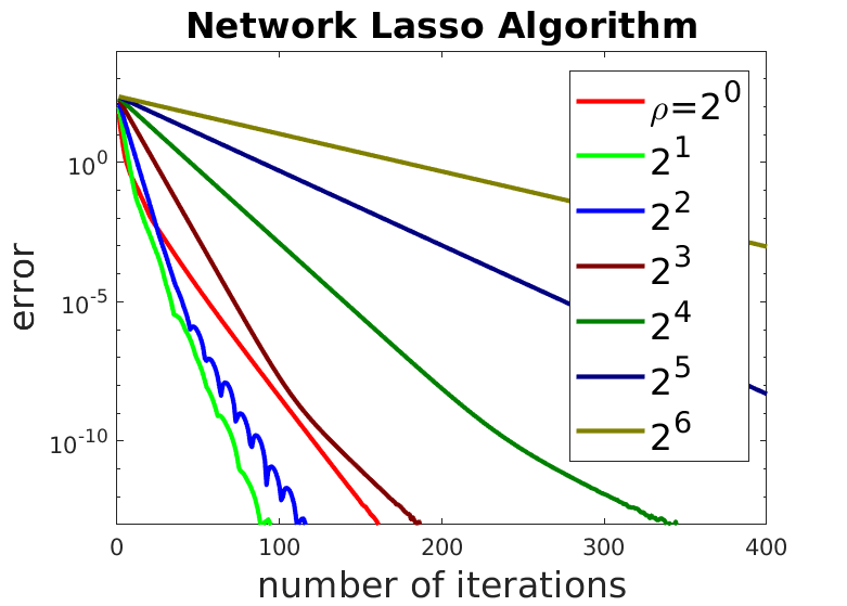
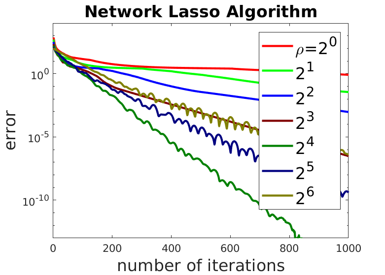
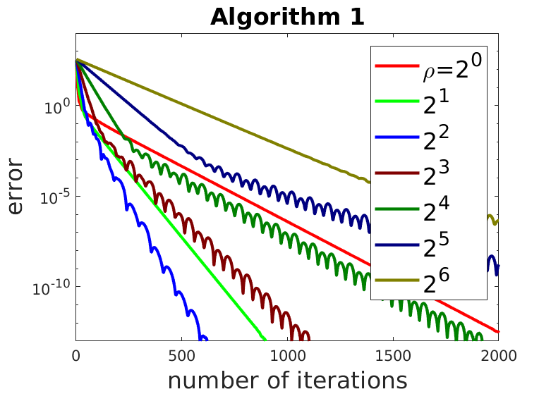
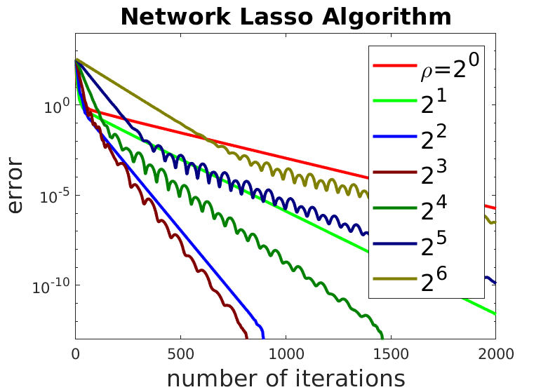
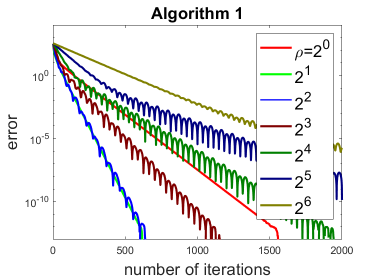
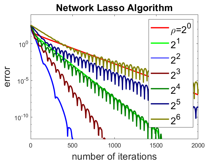
Then we let $\mathbf{y}_{i}=\mathbf{y}_{i}^{*}+N(\mathbf{0},\mathbf{I}_{2\times 2})$ and $\lambda=1$ or $10$, and compare Algorithm 1 will be compared with network lasso in Figure 2 with various choices of $\rho$. The figures indicate that for both choices of $\lambda$, Algorithm 1 always performs better with a good choice of $\rho$. In fact, if $\rho$ is chosen to be the optimal values for both algorithms, Algorithm 1 converges twice as fast as network lasso.

We also test the two-dimensional grid graph example. We generate data in the form of a $64$ by $64$ grid of points; the value is equal to $[0,0,0]$ for points within a distance of $16$ from the middle of the grid, and $[0.4,0.7,1]$ for all other points, and add noise of $N(\mathbf{0},\mathbf{I}_{3\times 3})$ for all points. For this example, we have a natural choice of $\mathcal{E}_{0}$ as visualized in the right Figure of Figure 3. The convergence rates are shown in Figure 4, which shows that Algorithm 1 has a comparable or faster convergence rate as the network lasso algorithm ADMM. Combining it with the fact that Algorithm 1 has a smaller computational complexity per iteration, this implies the numerical superiority of Algorithm 1.

We also use an example of a graphical fused lasso problem with a reasonably large, geographically-defined underlying graph. The data comes from police reports made publicly available by the city of Chicago, from 2001 until the present (Chicago Police Department 2014) and is available as the supplementary files of (Arnold and Tibshirani 2016). In this dataset, the vertices represent the census blocks and the edges represent the neighboring blocks, and more detailed explanation of this dataset is deferred to the supplementary file. This graph has $2162$ vertices, $6995$ edges and by running the greedy algorithm as described in Section 2.2, we obtain $\mathcal{E}_{0}$ with $1025$ edges and $\tilde{m}_{0}=797$. The result of the experiment in Figure 5 shows when $\lambda=0.05$ or $0.25$, Algorithm 1 converges much faster than the network lasso algorithm. Since Algorithm 1 has a smaller computational complexity per iteration as analyzed, this experiment shows that our algorithm numerically converges faster than network lasso.

Let us consider the problem

and its associated Lagrangian of

as well as the ADMM algorithm of

It can be verified that the update of (23)-(25) with $\bar{L}_{\rho}$ is in fact identical to the update of (10)-(12) with $\hat{L}_{2\rho}$. In addition, using the fact that (20) is (14) with additional constraints $\mathbf{z}_{ts}=\mathbf{x}_{s}+\mathbf{x}_{t}$, and Lemma 5.1 implies the equivalence between (23)-(25) is identical to (17)-(19).

References

• Arnold and Tibshirani (2016) Arnold, T. B. and R. J. Tibshirani (2016). Efficient implementations of the generalized lasso dual path algorithm. Journal of Computational and Graphical Statistics 25(1), 1–27.
• Barbero and Sra (2014) Barbero, A. and S. Sra (2014). Modular proximal optimization for multidimensional total-variation regularization.
• Bleakley and Vert (2011) Bleakley, K. and J.-P. Vert (2011, June). The group fused Lasso for multiple change-point detection. working paper or preprint.
• Boyd et al. (2011) Boyd, S., N. Parikh, E. Chu, B. Peleato, and J. Eckstein (2011, January). Distributed optimization and statistical learning via the alternating direction method of multipliers. Found. Trends Mach. Learn. 3(1), 1–122.
• Chambolle and Darbon (2009) Chambolle, A. and J. Darbon (2009). On total variation minimization and surface evolution using parametric maximum flows. International Journal of Computer Vision 84(3).
• Chen et al. (2012) Chen, X., Q. Lin, S. Kim, J. G. Carbonell, and E. P. Xing (2012, 06). Smoothing proximal gradient method for general structured sparse regression. Ann. Appl. Stat. 6(2), 719–752.
• Condat (2013) Condat, L. (2013, Nov). A direct algorithm for 1-d total variation denoising. IEEE Signal Processing Letters 20(11), 1054–1057.
• Davies and Kovac (2001) Davies, P. L. and A. Kovac (2001, 02). Local extremes, runs, strings and multiresolution. Ann. Statist. 29(1), 1–65.
• Eckstein and Bertsekas (1992) Eckstein, J. and D. P. Bertsekas (1992, Apr). On the douglas—rachford splitting method and the proximal point algorithm for maximal monotone operators. Mathematical Programming 55(1), 293–318.
• Friedman et al. (2007) Friedman, J., T. Hastie, H. Höfling, and R. Tibshirani (2007, 12). Pathwise coordinate optimization. Ann. Appl. Stat. 1(2), 302–332.
• Hallac et al. (2015) Hallac, D., J. Leskovec, and S. Boyd (2015, aug). Network Lasso: Clustering and Optimization in Large Graphs. KDD : proceedings. International Conference on Knowledge Discovery & Data Mining 2015, 387–396.
• Johnson (2013) Johnson, N. A. (2013). A dynamic programming algorithm for the fused lasso and l 0-segmentation. Journal of Computational and Graphical Statistics 22(2), 246–260.
• Kolmogorov et al. (2016) Kolmogorov, V., T. Pock, and M. Rolinek (2016). Total variation on a tree. SIAM Journal on Imaging Sciences 9(2), 605–636.
• Kovac and Smith (2011) Kovac, A. and A. D. A. C. Smith (2011). Nonparametric regression on a graph. Journal of Computational and Graphical Statistics 20(2), 432–447.
• Landrieu and Obozinski (2017) Landrieu, L. and G. Obozinski (2017). Cut pursuit: Fast algorithms to learn piecewise constant functions on general weighted graphs. SIAM Journal on Imaging Sciences 10(4), 1724–1766.
• Lin et al. (2014) Lin, X., M. Pham, and A. Ruszczynski (2014). Alternating linearization for structured regularization problems.  15, 3447–3481.
• Liu et al. (2010) Liu, J., L. Yuan, and J. Ye (2010). An efficient algorithm for a class of fused lasso problems. In Proceedings of the 16th ACM SIGKDD International Conference on Knowledge Discovery and Data Mining, KDD ’10, New York, NY, USA, pp. 323–332. ACM.
• Ramdas and Tibshirani (2015) Ramdas, A. and R. J. Tibshirani (2015, August). Fast and Flexible ADMM Algorithms for Trend Filtering. Journal of Computational and Graphical Statistics 25(3), 839–858.
• Rudin et al. (1992) Rudin, L. I., S. Osher, and E. Fatemi (1992). Nonlinear total variation based noise removal algorithms. Physica D: Nonlinear Phenomena 60(1), 259 – 268.
• Tansey and Scott (2015) Tansey, W. and J. G. Scott (2015, may). A Fast and Flexible Algorithm for the Graph-Fused Lasso.
• Tibshirani et al. (2005) Tibshirani, R., M. Saunders, S. Rosset, J. Zhu, and K. Knight (2005). Sparsity and smoothness via the fused lasso. Journal of the Royal Statistical Society Series B, 91–108.
• Wahlberg et al. (2012) Wahlberg, B., S. Boyd, M. Annergren, and Y. Wang (2012). An admm algorithm for a class of total variation regularized estimation problems. In Preprints of the 16th IFAC Symposium on System Identification, pp. 83–88. QC 20121112.
• Xu et al. (2017) Xu, Z., M. A. T. Figueiredo, and T. Goldstein (2017). Adaptive admm with spectral penalty parameter selection. In AISTATS.
• Ye and Xie (2011) Ye, G.-B. and X. Xie (2011). Split bregman method for large scale fused lasso. Computational Statistics & Data Analysis 55(4), 1552 – 1569.
• Yu et al. (2015) Yu, D., J.-H. Won, T. Lee, J. Lim, and S. Yoon (2015). High-dimensional fused lasso regression using majorization-minimization and parallel processing. Journal of Computational and Graphical Statistics 24(1), 121–153.
• Zhu (2017) Zhu, Y. (2017). An augmented admm algorithm with application to the generalized lasso problem. Journal of Computational and Graphical Statistics 26(1), 195–204.