Anisotropic layer construction of anisotropic fracton models
Abstract
We propose a coupled-layer construction of a class of fracton topological orders in three spatial dimensions, which has no immobile excitations but is characterized by single quasiparticle excitations constrained in one-dimensional subspaces and dipole excitations mobile in two-dimensional subspaces. The simplest model is obtained by stacking and coupling layers of the two-dimensional toric codes on the square lattice and can be exactly solved in the strong-coupling limit. The resulting subdimensional excitations are understood as a consequence of anyon pair condensation induced by the coupling between layers. We also present generalizations of the construction for layers of the Kitaev-honeycomb models, the toric codes, and the toric codes and the doubled semion models on the honeycomb lattice.
I Introduction
A peculiar phenomenon in strongly interacting many-body quantum systems is the emergence of fractionalized quasiparticles as low-energy collective excitations. In two dimensions, topologically ordered states, such as the fractional quantum Hall states, support point-like quasiparticles with nontrivial braiding statistics of neither fermion nor boson Wen 2016. In three dimensions, fractionalized quasiparticles appear in the shape of point or loop and can have nontrivial statistics among them Hamma et al. 2005; Wang and Levin 2014; Jiang et al. 2014; Lin and Levin 2015; Wang and Wen 2015. These topologically ordered phases are characterized by quasiparticles deconfined in the full two-dimensional () or three-dimensional () space, and their presence results in a finite ground-state degeneracy on a torus or other nontrivial closed manifolds, which is robust against any local perturbations.
Recently, a new class of topological phases of matter in three dimensions, dubbed fracton topological order Vijay et al. 2016, has been discovered and offers a rapidly growing field of theoretical research Chamon 2005; Bravyi et al. 2011; Haah 2011; Yoshida 2013; Vijay et al. 2015; Vijay et al. 2016; Williamson 2016; Halász et al. 2017; Ma et al. 2017; Petrova and Regnault 2017; Prem et al. 2017; Pretko 2017a; Pretko 2017b; Pretko 2017c; Slagle and Kim 2017a; Slagle and Kim 2017b; Hsieh and Halász 2017; Vijay; Vijay and Fu; Shi and Lu 2018; Bulmash and Barkeshli a; Bulmash and Barkeshli 2018; Devakul et al. 2018; Gromov; Ma et al. 2018a; Ma et al. 2018b; He et al. 2018; Pai and Pretko 2018; Prem et al. 2018a; Prem et al. 2018b; Pretko and Radzihovsky 2018a; Pretko and Radzihovsky 2018b; Schmitz et al. 2018; Shirley et al. a; Shirley et al. 2018; Slagle and Kim 2018; Williamson et al.; You et al. a; You et al. b; You and von Oppen; Bulmash and Iadecola 2019; Bulmash and Barkeshli b; Dua et al. 2019; Gromov 2019; Yan 2019; Yan; Song et al. 2019; Tian and Wang; Pai and Hermele; Prem et al. 2019; Prem and Williamson; Shirley et al. 2019a; Shirley et al. 2019b; Shirley et al. b; Slagle et al. 2019; Sous and Pretko; Wang et al.; You et al. c; see also a review Nandkishore and Hermele 2019. Quasiparticle excitations emerging from such fracton topological phases are completely immobile or mobile only within lower-dimensional subspaces of the full space; the former are called fractons, while the latter are called lineons or planons depending on their mobility. The restricted mobility of quasiparticles in gapped fracton phases causes a ground-state degeneracy that is sensitive to the geometry of the system and often exponentially grows with increasing of the system size, but the degeneracy is still topologically stable in the sense that it cannot be split by local perturbations.
Since both geometry and topology essentially come into play, the fracton topological phases fall outside of the effective description in terms of topological quantum field theory commonly used for conventional topologically ordered phases. The fracton phases rather require some lattice description and in fact many key properties of gapped fracton phases have been established upon the construction of exactly solvable lattice models, which often consist of local commuting projectors. There have been several proposed schemes to obtain such lattice models, including the construction from coupled layers of topological phases Ma et al. 2017; Vijay; Vijay and Fu; Slagle and Kim 2017a; Prem et al. 2019; Shirley et al. b, spin chains Halász et al. 2017, Majorana fermions Hsieh and Halász 2017; You et al. b; You and von Oppen, string-membrane-net condensation Slagle et al. 2019, and gauging of associated symmetry-protected topological phases Vijay et al. 2016; Williamson 2016; Williamson et al.; You et al. a; Shirley et al. 2019b. Especially to realize fracton topological phases in experiment, the construction from constituents naturally appearing in materials will be much desired.
In this paper, we propose a coupled-layer construction of fracton topological phases, which differs from those developed previously Ma et al. 2017; Vijay; Prem et al. 2019; Shirley et al. b; instead of stacking layers of topological orders in all three orthogonal directions of the space, our construction requires a stack of topological orders only in one direction. With appropriate couplings to implement anyon condensation between layers, the corresponding models undergo phase transitions from decoupled topological phases to fracton topological phases. The resulting fracton phases have quasiparticles with spatially anisotropic mobility, in contrast to the “isotropic” layer constructions Ma et al. 2017; Vijay; Prem et al. 2019; Shirley et al. b which yield the X-cube model Vijay et al. 2016 or their relatives with the same mobility of quasiparticles in all three directions. While our models lack fractons as strictly immobile excitations, the models exhibit lineons constrained in one-dimensional subspaces, whose dipoles behave as planons mobile in two-dimensional subspaces 11 1 As a remark, while our models do not possess “fractons” as strictly immobile excitations, we abuse “fracton models” or “fracton topological orders” to emphasize that the corresponding models are still distinguished from the conventional topological orders or their decoulpled stacks.. In the special case of stacked toric codes on the square lattice, the models in the strong-coupling limit turn out to be described by exactly solvable models proposed by Shirley, Slagle, and Chen in Ref. Shirley et al. a. As the models obtained by our construction take simpler forms than the previous models, they may help us to seek experimental realizations of fracton topological orders, e.g., in spin-liquid candidate materials with “bad” two-dimensionality.
The rest of paper is organized as follows: In Sec. II, we review anyon condensations and their model realizations in the toric code Kitaev 2003. In Sec. III, we present the simplest model consisting of stacked layers of the toric codes on the square lattice, whose quasiparticle excitations in a fracton phase are analyzed in the strong-coupling limit or understood from the perspective of anyon condensation. In Sec. IV, we propose generalizations of the construction for stacked layers of other lattice models. We conclude our paper with several discussions in Sec. V.
II Anyon condensation in the toric code
Prior to addressing the construction of anisotropic fracton models from coupled layers of topological orders, we first consider anyon condensation transitions in a single layer or a bilayer of the toric code. This will be helpful on later interpreting the anisotropic mobility of quasiparticles in fracton phases as a result of anyon condensation and will also give us insights on how to construct the corresponding lattice Hamiltonians.
II.1 toric code
Let us first review properties of the toric code on the square lattice Kitaev 2003. We consider the system of qubits put on each link of the square lattice. The Hamiltonian is given by
| (1) |
where the operators and are defined on each plaquette () or vertex () on the square lattice by
| (2) | ||||
| (3) |
Here, we have defined and as the Pauli operators acting on a qubit on the link , and the products are taken over four links forming a plaquette or vertex . The Hamiltonian is pictorially given in Fig. 1 (a).
Since the operators and satisfy and , the ground state is obtained as a simultaneous eigenstate of and whose eigenvalues are all . However, not all operators can span the Hilbert space when the system is placed on a torus, due to the constraints and , which result in the -fold degeneracy of the ground state. This ground-state degeneracy is topological in the sense that it cannot be lifted by any local perturbations; as the ground-state manifold is spanned by nonlocal string operators of or winding noncontractible cycles of the torus, splitting of the degeneracy by local perturbations is exponentially suppressed with increasing the system size.
There are two types of excitations from the ground state. As depicted in Fig. 1 (b), acting an open string of creates a pair of excitations at the ends of the string, where the eigenvalues of are flipped to be . Similarly, an open string of creates a pair of excitations at the ends of the string, where the eigenvalues of are flipped. These excitations are deconfined since the excitation energy remains constant regardless of the length of the string. We may call the excitations created by electric charges , as they live on the vertices, while those created by magnetic charges , as they live on the plaquettes. Writing their bound object as and the vacuum as , the toric code has the four quasiparticles:
| (4) |
The same species of quasiparticles fuse to the vacuum, . While and are bosons on their own, they have the nontrivial mutual statistics of since two string operators of and intersect once and pick up a phase when () goes around (). As a result, their bound object behaves as a fermion. They then have the fusion rules , , and . This is known as the topological order.
II.2 Condensation in a single layer
We here review phase transitions induced by anyon condensation in a single layer of the toric code. The concept of anyon condensation was introduced by Bais and Slingerland Bais and Slingerland 2009 in order to discuss phase transitions between topological orders driven by the condensation of bosonic quasiparticles, and several systematic approaches to identifying the topological orders in condensed phases have been developed Eliëns et al. 2014; Kong 2014; Neupert et al. 2016; see also a recent review Burnell 2018. In the case of the toric code, there are two types of bosonic quasiparticle, and , either of which can be condensed. In the condensate, remaining quasiparticles and both have the nontrivial mutual statistics of with respect to and thus are confined; the resulting state has a trivial topological order. Similarly, the condensation of also leads to a trivial topological order.
Let us consider microscopic models exemplifying these anyon condensation transitions. As reviewed in Sec. II.1, excitations are created by acting the Pauli operator ’s on the ground state of the toric-code Hamiltonian (1), while excitations are created by acting ’s. Hence, the condensation of or will be simply induced by applying magnetic fields to the toric code:
| (5) | ||||
| (6) |
We expect that the magnetic field induces an -condensation transition while induces an -condensation transition. Obviously, the ground state becomes a fully polarized state with a trivial topological order in the limit of large or , and thus there will be a phase transition between the and trivial topological orders for some or . In fact, these models have been studied previously Trebst et al. 2007; Vidal et al. 2009; Tupitsyn et al. 2010; Dusuel et al. 2011; Wu et al. 2012; the corresponding phase transitions are conjectured to be in the (2+1)- Ising∗ universality class—the Wilson-Fisher fixed point of a real scalar field theory coupled with a gauge field Schuler et al. 2016.
II.3 Condensation between two layers
We then focus on two layers of the toric codes. When the two layers are decoupled, the ground state has a topological order with 16 quasiparticles given by
| (7) |
where the subscripts and refer to the two layers and the quasiparticles are simply given by tensor products of those from each layer. We then consider phase transitions induced by the condensation of bound pairs of quasiparticles between the two layers. For examples, is a boson and thus can be condensed. In the condensate, all quasiparticles obeying nontrivial mutual statistics with are confined. We are thus left with a topological order characterized by the following quasiparticles:
| (8) |
Here, quasiparticles that are transformed to each other by the fusion with are identified. The resulting topological order has four quasiparticles, and their statistics exactly matches with that for a single layer of the toric code; we thus call it as and label the quasiparticles by symbols with a tilde.
We want to implement this phenomenology of the topological phase transition from to in a microscopic model. Taking a bilayer of the toric code, a bound pair of ’s from each layer may be created by the action of where the Pauli operator acts on a qubit on the link of the layer . We thus consider the Hamiltonian,
| (9) |
where
| (10) |
Again, the labels and refer to the plaquettes and vertices of the square lattice, respectively, as shown in Fig. 1 (a). The structure of the coupling between layers is schematically given in Fig. 2 (a).
In order to see that this Hamiltonian exhibits the expected phase transition, we now consider the strong-coupling limit . In this limit, the two qubits on the same link are in either of two states, or , in the basis diagonalizing , i.e. . Let us denote by two basis states of an effective qubit on the link . We then perform degenerate perturbation theory in the Hilbert space of effective qubits by treating as perturbations. In doing so, we define the Pauli operators and acting on the effective qubits and choose to be diagonal, i.e. and . Projecting the original Pauli operators into the subspace spanned by effective qubits, we find and . Up to the second order in perturbation, we arrive at the effective Hamiltonian,
| (11) |
This Hamiltonian is equivalent to that for the toric code up to a unitary transformation. Since the ground state is expected to have the topological order for a large enough , we conclude that the Hamiltonian (9) describes a phase transition from to induced by the condensation.
For the condensation in , the quasiparticle content in the condensate is given by
| (12) |
and is the same as that for a single layer of the toric code. As the Pauli operator creates excitations on each layer, the corresponding Hamiltonian may be given by
| (13) |
as shown in Fig. 2 (b). In the strong-coupling limit , we can introduce the basis states for effective qubits as where we have chosen the original basis to be . By performing degenerate perturbation theory, we find the effective Hamiltonian
| (14) |
where we have defined the Pauli operators acting on the effective qubits in such a way that and . This is again a single layer of the toric code, although this result is not surprising from the - duality in the toric code. Thus, the Hamiltonian (13) will describe a topological phase transition induced by the condensation.
Before proceeding, we make a remark about the nature of the transitions. While it is not so obvious, the transition from to induced by the or condensation is expected to be in the Ising∗ universality class as in the single-layer case. This is because the transition in the bilayer can be viewed as a single-layer transition from the to trivial topological order from its quasiparticle content; we can rewrite the quasiparticle content of as
| (15) |
where the multiplication should be operated in the sense of fusion. Since the two sets of quasiparticles both represent the topological order while the statistics of quasiparticles are mutually trivial between the two sets, we can regard them as two decoupled layers of the topological orders. The or condensation is simply viewed as the single or condensation in one layer with leaving another layer intact. Therefore, the associate transition is naturally expected to be of the Ising∗ type.
III Fracton model from coupled toric codes
We present a model that may have an anyon condensation transition from decoupled layers of the toric codes to a nontrivial fracton topological order. In the limit of strong coupling between layers, we can write down an effective Hamiltonian that is exactly solvable. In fact, the resulting model has been proposed in Ref. Shirley et al. a and possesses fractionalized quasiparticles with spatially anisotropic mobility, which is yet different from that of the stacked toric codes. We argue that the anisotropic mobility of quasiparticles can be naturally explained in terms of anyon condensation induced by coupling between the toric codes.
III.1 Model
We consider layers of the toric code lying in the plane and stacked along the axis, which are given by the Hamiltonian,
| (16) |
where is the Hamiltonian for the toric code on the -th layer and is defined in Eq. (10). We then consider coupling between layers that takes a staggered structure as follows: Two qubits from the -th and ()-th layers are coupled via on the link aligned with the axis, whereas two qubits from the ()-th and -th layers are coupled via on the link aligned with the axis. The corresponding Hamiltonian is given by
| (17) |
which is schematically shown in Fig. 3 (a).

The full Hamiltonian for the coupled toric codes is then given by
| (18) |
The ground state obviously has the topological order of decoupled toric codes for , which is characterized by quasiparticles of the topological order deconfined only within each layer and the ground-state degeneracy on a three-torus with layers. The model is no longer exactly solvable for a general choice of the parameters. However, an effective Hamiltonian obtained in the strong-coupling limit is exactly solvable as we will see below.
III.2 Strong-coupling limit: Anisotropic fracton model
In the spirit of Sec. II.3, we here derive an effective Hamiltonian in the strong-coupling limit . In the limit , two qubits on the link parallel to the axis form either of the two states between the -th and ()-th layers,
| (19) | ||||
in the basis where is diagonalized: . In the limit , two qubits on the link parallel to the axis form either of the two states between the ()-th and -th layers,
| (20) | ||||
| (21) |
in the basis where is diagonalized: . We now treat the toric-code Hamiltonian in Eq. (16) as a perturbation and perform degenerate perturbation theory to obtain an effective Hamiltonian acting on the Hilbert space of effective qubits . By squashing the and bonds between layers to points, these effective qubits can be viewed to live on a bcc lattice as shown in Fig. 3 (b); let us denote by the sublattice a cubic lattice composed of effective qubits on the ()-th layers, which used to be defined on the bonds of the coupled toric codes, whereas by the sublattice another cubic lattice composed of effective qubits on the ()-th layers, which used to be defined on the bonds. We then introduce the Pauli operators and acting on the effective qubit at the site on the () sublattice of the bcc lattice. After the projection onto the Hilbert space of effective qubits, the original Pauli operators and can be represented as
| (22) | ||||
for , while
| (23) | ||||
for .
Up to the second order in , we find the effective Hamiltonian acting on effective qubits,
| (24) |
where denotes a face of a cube that belongs to either or sublattice and is parallel to the plane, and and are local operators defined by
| (25) | ||||
As seen from Fig. 3 (c), the operator is a product of four operators on the sublattice at the corners of the face and two operators on the sublattice at the ends of a bond normal to the face , and similarly for by interchanging the and sublattices. The same Hamiltonian as Eq. (24) has been previously introduced in Ref. Shirley et al. a for an anisotropic fracton model. While basic properties of the Hamiltonian have already been discussed in the same reference, we review below those properties in detail for completeness.
III.2.1 Ground-state degeneracy
As any two operators from and commute, the effective Hamiltonian (24) is exactly solvable. Since , the ground state is given by a simultaneous eigenstate of and whose eigenvalues are all . Similarly to the toric code, there can be constraints that make certain products of the operators and to be the identity, leaving the ground-state degeneracy. Let us consider the system put on a three-torus with the linear sizes such that there are effective qubits. We may first multiply along the axis to cancel the operators. Residual operators form a “tube” along the axis and can be multiplied along either the or axis to be the identity. We thus find the following constraints,
| (26) |
meaning that ’s multiplied over the or plane become the identity. Similarly, we also have
| (27) |
There are in total independent conditions, which result in the subextensive ground-state degeneracy
| (28) |
The subextensive degeneracy is a signal of fracton topological order. However, we have to make sure that this degeneracy cannot be split by local perturbations. In order to see this, we here show that logical operators spanning the ground-state manifold have nonlocal supports that grow with increasing the systems size. This implies that splitting of degenerate ground states by local perturbations vanishes in the thermodynamic limit. There are line-like logical operators composed of the Pauli operators on the sublattice along the axis,
| (29) |
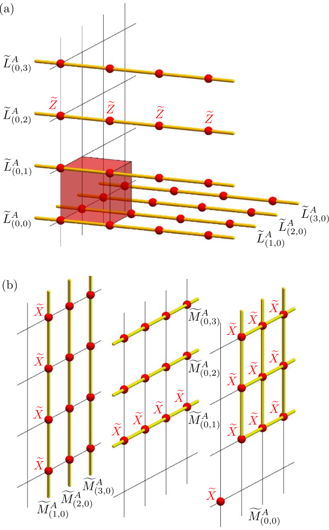
where denotes the coordinates on the cubic lattice. These operators commute with all terms in the Hamiltonian (24). If a product of the operators forms a quadrangular prism whose base is a rectangle on the plane, it can be written in terms of a product of and trivially acts on the ground state. Thus, there are only independent line-like operators nontrivially acting on the ground state. For our convenience, we make the following choice for the coordinates of such line-like operators,
| (30) |
as shown in Fig. 4 (a).
In addition, there are also “membrane-like” logical operators composed of the Pauli operators on the sublattice in a plane,
| (31) | ||||
as shown in Fig. 4 (b). Here, the choice of is arbitrary since can be shifted along the axis by multiplying operators . Again, they commute with all terms in the Hamiltonian and nontrvially act on the ground state. Upon our choice, the line-like operators and membrane-like operators anticommute for the same but commute for different ’s:
| (32) |
We can similarly construct the line-like and membrane-like operators on the sublattice for which a similar algebra holds. These sets of logical operators span the -dimensional Hilbert space of the degenerate ground-state manifold. Importantly, these logical operators cannot be multiplied to form any local operators. This implies that a matrix element between degenerate ground states is generated by local perturbations at least at the order of , , or and is expected to vanish in the thermodynamic limit. This ensures a topological stability of the subextensive degeneracy and thereby a fracton topological order.
III.2.2 Subdimensional excitations
The subextensive ground-state degeneracy computed above is a consequence of deconfined excitations restricted in lower-dimensional subspaces of the space. Since the local terms in the Hamiltonian, and , have eigenvalues in the ground state, excited states are obtained by flipping some of the eigenvalues by acting a local operator on the ground state. As the operators () are centered at faces of cubes that belong to the () sublattice and are parallel to the plane, we may regard that excitations are created on these faces. Depending on the mobility of excitations, which we will see below, they are called “lineons” or “planons” in Ref. Shirley et al. a.
Acting a Pauli operator on the ground state, it creates excitations on two faces of the sublattice sandwiching the site . By successively applying Pauli operators, a single excitation can be transferred on a straight line along the axis. From its one-dimensional nature, every single excitation is called a lineon. On the other hand, when two pairs of lineon excitations are created within a plane, a dipole of excitations separated along the axis can be transferred along the axis by successively applying Pauli operators to form a rectangular membrane in the plane; such a membrane operator by itself creates four excitations at the corners of the rectangle. Hence, the dipole freely moves within the plane. Similarly, a dipole of excitations separated along the axis can move in the plane. Thus, dipoles of excitations have a nature and are called planons. A way of creating such excitations is illustrated in Fig. 5.
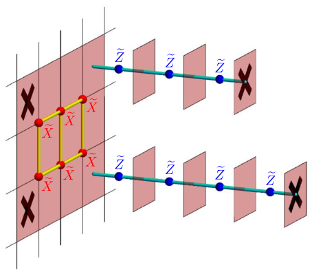
Similarly, we can create lineon and planon excitations living on faces of the sublattice by applying Pauli and operators. In fact, a finite segment of the line-like operator creates a pair of lineon excitations along the axis, while a portion of the membrane-like operator creates a pair of dipole excitations in the plane. When excitations are annihilated in pairs by wrapping the torus, the corresponding nonlocal operators map the ground-state manifold to itself and define logical operators ’s or ’s. As the excitations behave in quite different ways between the three spatial directions, the model (24) is dubbed as the anisotropic fracton model.
III.3 Anyon condensation picture
We can interpret the spatially anisotropic mobility of subdimensional excitations beyond the strong-coupling limit in the view of anyon condensation in the coupled toric-code model (18). Taking a slice of the model in the plane, as shown in Fig. 6 (a), let us consider the mobility of an excitation created on a vertex by acting the Pauli operator.
Along the axis, the couplings induce the condensation between adjacent layers for a certain strength of . As has the trivial mutual statistics with , a single excitation can go through the condensate, as shown in the left panel of Fig. 6 (b); this may be viewed as the origin of lineon excitations on the sublattice. On the other hand, the couplings run along the axis and induce the condensation between adjacent layers for a certain . Since has the nontrivial mutual statistics of with , excitations must form a bound pair between the adjacent layers to move in the condensate, as shown in the right panel of Fig. 6 (b); this explains the dipole nature of excitations along the axis on the sublattice. When these dipoles of excitations are created successively over several layers, the excitations in internal layers become invisible due to the formation of condensate and only excitations on the top and bottom layers are left; this establishes the dipole nature of excitations along the axis, and together with the above arguments we find planon excitations in the or plane. The same phenomenology also applies to excitations, which see the condensate along the axis while the condensate along the axis, leading to lineon and planon excitations on the sublattice.
IV Generalization
We here generalize the construction of the anisotropic fracton model to coupled layers of other lattice models: the Kitaev honeycomb model, the toric code, and the toric code and the doubled semion model on the honeycomb lattice.
IV.1 Kitaev-honeycomb model
Since the anisotropic fracton model (24) is obtained from stacked layers of the toric codes on the square lattice, it should be possible to realize the same model from stacked layers of the Kitaev honeycomb model Kitaev 2006, as it gives the toric code in the easy-axis limits. The idea of constructing fracton topological order from stacked layers of the Kitaev honeycomb models has already appeared in Ref. Slagle and Kim 2017a, where stacks in two spatial directions have been used to obtain the X-cube model. Our construction is relatively simple as it only requires a stack in one direction. Let us consider the following Hamiltonian,
| (33) |
where is the Kitaev honeycomb model on the -th layer,
| (34) |
and () are the Pauli operators at the site of the honeycomb lattice on the layer . As illustrated in Fig. 7, the three couplings are assigned for three different bonds on each layer of the honeycomb lattice, and we further assign the - and -links to implement the desired staggered layer structure.

As is well known, a single layer of the Kitaev honeycomb model produces the toric code on the square lattice in the strong-coupling limit of, say, on the -bonds. In this limit, we may define effective spin-’s on -bonds by and where and . These effective spins on each layer now form the square lattice and the spins are defined on the vertices of the square lattice. The - and -links in the Hamiltonian (IV.1) then belong to each of two sublattices of the square lattice. Performing degenerate perturbation theory in the limit , we obtain the effective Hamiltonian,
| (35) |
where we have defined the Pauli operators , , and acting on the effective spin at the vertex on the layer . The first sum is taken over plaquettes of the square lattice on each layer, and l(), u(), r(), and d() indicate four corners surrounding the square plaquette in the clockwise Kitaev 2006. This effective Hamiltonian is unitarily equivalent to the model defined in Eq. (18) and one can find that the following unitary transformation does the job:
| (36) |
We remark that since we have only kept the first-order terms in in Eq. (IV.1) the parameters of the original Kitaev honeycomb model must be appropriately tuned such that only the terms remaining in Eq. (IV.1) are dominant. On the other hand, the couplings between adjacent layers are not restrictive to the form in Eq. (IV.1) but can be, e.g., of the Heisenberg type as far as lowest order perturbations are considered.
One can also directly work on the strong-coupling limit and derive the anisotropic fracton model (24) acting on effective qubits , formed by four spins connected by the and bonds in lowest-order perturbation theory. Although the Kitaev honeycomb model can be exactly solved by introducing the Majorana representation of spins Kitaev 2006, the additional couplings between layers make the model not solvable and may require some mean-field treatment to fully explore the phase diagram.
IV.2 toric code
It is straightforward to generalize the construction in Sec. III to coupled layers of the toric code Kitaev 2003. Let us define the generalized Pauli operators and satisfying with , which act on the local Hilbert space of a qudit () as and . We then consider stacked layers of the toric code on the square lattice where qudits are defined on each link and introduce couplings between layers to implement anyon condensation. In analogy with Eq. (18), the corresponding Hamiltonian is given by
| (37) |
where is the toric code Hamiltonian on the -th layer,
| (38) |
The local terms and are defined by
| (39) | ||||
The Hamiltonian is schematically shown in Fig. 8 (a).

When , the Hamiltonian is just decoupled layers of the toric code, which is exactly solvable. As the Hamiltonian consists of local commuting terms and , the ground state is given by a simultaneous eigenstate of and with the eigenvalues . By acting an operator on the ground state, it creates a pair of and excitations on neighboring vertices, and similarly creates a pair of and on neighboring plaquettes. Each layer hosts quasiparticles of the topological order given by and and their bound objects. Here, and are bosons but have the nontrivial mutual statistics of ; the quasiparticle or () are obtained by fusing ’s or ’s, respectively, while fusing ’s or ’s leads to the vacuum .
A finite coupling will induce the condensation of - pairs between adjacent layers, while will induce the condensation of - pairs. A single excitation created on a vertex of a layer can propagate through the - condensate along the axis, and similarly a single created on a plaquette propagate through the - condensate along the axis; they behave as lineon excitations. On the other hand, the excitation sees the - condensate in the direction, and it must form an - pair with the neighboring layer to move along the axis. Similarly, only an - pair can move along the axis. Thus, dipoles of ’s or ’s separated along the axis behave as planon excitations in the plane. Finally, when - pairs and - pairs are alternatively created over several layers, the internal - pairs become invisible in the - condensate and only dipoles of and separated along the axis are left at the top and bottom layers. This dipole nature similarly applies to excitations. Such dipoles behave as planons in the plane.
This phenomenology from anyon condensation can be explicitly seen in the effective Hamiltonian obtained in the strong-coupling limit . In this limit, two qudits on a link parallel to the axis are in one of the following states labeled by ,
| (40) |
in the basis satisfying , while for those on a link parallel to the axis we have
| (41) |
in the basis satisfying . As in Sec. III.2, the effective qudits live on the bcc lattice. We can then perform degenerate perturbation theory and obtain an effective Hamiltonian acting on the Hilbert space of the effective qudits,
| (42) |
where the local terms and are defined by
| (43) | ||||
as shown in Fig. 8 (b). Here, we have defined generalized Pauli operators, and , acting on an effective qudit at the site on the () sublattice of the bcc lattice: and . The Hamiltonian (IV.2) has also been introduced in Ref. Shirley et al. a and is again exactly solvable. The ground state admits lineon and planon excitations as discussed above from the view of anyon condensation, resulting in the ground-state degeneracy on a torus.
IV.3 Toric code on the honeycomb lattice
We can generalize the coupled-layer construction of the anisotropic fracton model in Sec. III to the toric codes defined on trivalent graphs. Here, let us specifically focus on the honeycomb lattice. The coupled-layer model is defined by the Hamiltonian,
| (44) |
where is the toric code Hamiltonian on the -th layer,
| (45) |
Here, the Pauli operators and act on a qubit placed on the link of the honeycomb lattice on the -th layer. Since there are three inequivalent links under rotation, we specify them by the vectors as defined in Fig. 9 (a).

The local terms in Eq. (45) act on plaquettes with six links or vertices with three links as also shown in Fig. 9 (a). Similarly to the case for the square lattice, we implement a staggered structure of coupling between layers; links parallel to or are coupled via between the -th and -th layers, while those parallel to are coupled via between the -th and -th layers, as shown in Fig. 9 (b). We then perform degenerate perturbation theory in the strong-coupling limit and obtain the effective Hamiltonian for effective qubits on the vertical bonds,
| (46) |
We here regard that the effective qubits on links parallel to or form a cubic lattice as shown in Fig. 9 (c). The effective qubits on links parallel to live on the center of cubes to form a checkerboard pattern in the plane. The first sum in Eq. (46) is taken over cubes that do not contain the qubits on the links, whereas the second sum is taken over faces that are parallel to the plane and belong to cubes containing the qubits on the links. The local operators , , and are written in terms of products of Pauli operators and acting on the effective qubits, whose specific forms are pictorially shown in Fig. 9 (c).
The Hamitonian (46) is a commuting projector Hamiltonian and thus is exactly solvable. As we demonstrate below, it is a variant of the anisotropic fracton model considered above. We define the unit cell to contain three qubits from the links and consider the torus with effective qubits. As similarly seen in Sec. III.2.1, the local operators in the Hamiltonian do not fully span the Hilbert space and turn out to leave the ground-state degeneracy,
| (47) |
since the operators are multiplied over the or plane to be identity and similarly for and . This subextensive degeneracy is again a consequence of subdimensional excitations. Successively acting Pauli operators on links on a straight line along the axis, they flip the eigenvalues of on the line and create lineon excitations. However, their dipoles separated along the axis can move on the plane by acting Pauli operators on links and thus become planon excitations, as illustrated in Fig. 10 (a).

On the other hand, dipoles created within the plane become planon excitations moving on the plane [Fig. 10 (b)]. Acting Pauli operators on links along the axis, they flip the eigenvalues of and and create another type of lineon excitations. With the action of Pauli operators on links, their dipoles behave as planon excitations in the plane when they are separated along the axis [Fig. 10 (c)] or in the plane when they are separated along the axis [Fig. 10 (d)]. These anisotropic behaviors of quasiparticle excitations can also be understood from the view of anyon condensation as discussed in Sec. III.3 by taking account of the lattice and coupling structure accordingly.
It appears that we can obtain another anisotropic fracton model by interchanging the and couplings in Eq. (IV.3) and by taking the strong-coupling limit, although this makes just a rotation for the coupled-layer model defined on the square lattice in Sec. III. However, the degenerate perturbation theory generates local terms consisting of plaquette and vertex operators not only between adjacent layers but also within the same layer at the second order. These terms render the resulting model trivial up to a stack of topological orders. As discussed in Sec. V, this might be a generic feature of our construction when the coupling between layers makes the original quasiparicles (single ’s or ’s in the toric code) immobile within a layer.
IV.4 Doubled semion model
As we have constructed an anisotropic fracton model from coupled layers of the toric code on the honeycomb lattice, there might be generalizations to the string-net models Levin and Wen 2005, which provide exactly solvable Hamiltonians for various topological orders on trivalent graphs including the honeycomb lattice. One of the simplest models among them is the doubled semion model, which has been used for the coupled-layer construction of the semionic X-cube model Ma et al. 2017. We thus consider coupled layers of the doubled semion model on the honeycomb lattice,
| (48) |
Here, is the Hamiltonian for the doubled semion model on the -th layer,
| (49) |
where the first term consists of the Pauli operators acting on six links of the plaquette , the operators acting on six links coming into the plaquette, and the projection operators acting on six vertices of the plaquette to enforce the constraints on each vertex [see Fig. 11 (a)].

We have implemented the same structure of coupling between layers as in the case for the toric code.
Similarly to the toric code, a Pauli operator flips the eigenvalues of plaquette terms and thus create excitations on the plaquettes. These excitations can be seen as bosonic quasiparticles () in the doubled semion topological order Levin and Wen 2005. Therefore, the coupling in Eq. (IV.4) will induce the condensation of between adjacent layers. On the other hand, a Pauli operator does not solely flip the eigenvalues of vertex terms for the doubled semion model. In fact, the corresponding string operator must be appropriately modified to selectively excite semion () or anti-semion () excitations Levin and Wen 2005, and the action of a single operator rather yields a superposition of excited states with or . Thus, we cannot draw a clear picture from the anyon condensation induced by the coupling to discuss the motion of quasiparticles in this case. Nevertheless, we can write down the effective Hamiltonian in the strong-coupling limit , which takes the same form as Eq. (46) at the second-order with modified cube terms as illustrated in Fig. 11 (b). It still keeps a commuting-projector form and is exactly solvable. The ground-state degeneracy on the torus is also not changed from . Although the action of a single operator is changed as it creates excitations in as well as and , causing a slightly complicated behavior for dipole excitations, the model possesses quasiparticle excitations in the forms of lineons and planons essentially similar to those discussed in Sec. IV.3. Hence, what we have obtained from the doubled semion model is still a variant of the anisotropic fracton model.
V Conclusion and discussion
In this work, we have proposed a coupled-layer construction of anisotropic fracton models from layers of topological orders stacked in one spatial direction. Quasiparticle excitations in fracton phases have been studied by analyzing the effective Hamiltonians in the strong-coupling limit or by considering the pair condensation of quasiparticles of the original topological orders between adjacent layers. The subdimensional excitations show the spatially anisotropic mobility of lineons moving only along a straight line or planons moving only within a plane, depending on how the original quasiparticles on each layer see the anyon condensates induced by the coupling between layers.
We can then ask what happens when the anyon condensation between layers do not allow the original quasiparticles to move in isolation—the situation reminiscent of immobile, fracton excitations. For instance, let us consider two patterns of the and coupling between layers of the toric codes defined on the square or honeycomb lattice, as depicted in Fig. 12.
In such cases, either single or excitations cannot move, while another kind of excitations can move within a layer and can form closed loops around where the other excitations are trapped. Performing degenerate perturbation theory in the strong-coupling limit, we have two types of nonvanishing terms: One consists of the original plaquette and vertex terms between adjacent layers, while another consists of those within the same layer; the latter results from the presence of excitations moving along the loops. If we discard such intralayer terms in the effective Hamiltonian, the ground state on a torus has degeneracy exponentially scaling with , which is the number of closed loops. However, this degeneracy is lifted once the intralayer terms are added, leaving only the degeneracy coming from topological orders stacked along the direction. Thus, the resulting models become trivial as fracton topological order. In order to have nontrivial fracton models, the anyon condensation will necessarily be implemented in such a way that both and excitations can move along some one-dimensional paths. Such models will have lineons and planons as dipoles of the lineons, but no fractons. We expect that this is a generic feature of our construction using topological orders stacked only along one direction.
There are several other questions naturally raised: (i) Although we did not address the nature of transitions from decoupled topological orders to anisotropic fracton models, the duality mapping Vijay; Slagle and Kim 2017a suggests that the transition for the case is described by a stack of transverse Ising chains. Once those chains are coupled, the transition is expected to be first order or accompanied with an intermediate phase Slagle and Kim 2017a. Since the models are simpler than those obtained from the previous layer constructions Ma et al. 2017; Vijay; Vijay and Fu; Slagle and Kim 2017a; Prem et al. 2019; Shirley et al. b, direct numerical simulations may be more capable of determining the nature of the phase transitions. (ii) As a model has been obtained from a single stack of layers of the Kitaev honeycomb models in Sec. IV.1, it is interesting to seek possibilities to realize fracton orders in spin-orbit-coupled materials in the proximity to a spin liquid but with non-negligible couplings Jackeli and Khaliullin 2009; Chaloupka et al. 2010. (iii) There may be a generalization of the present layer construction for twisted cousins of the anisotropic fracton models as proposed for the X-cube model and others You et al. a; Song et al. 2019; Shirley et al. b.
The construction using topologically ordered phases stacked only in one direction bears a resemblance to the layer construction proposed for conventional topological orders or surface topological orders of topological phases Jian and Qi 2014. The simplest example of the latter construction requires the successive condensation of pairs between layers of the toric codes and is expected to give the topological order with bosonic point-like quasiparticles of and loop-like quasiparticles made of strings of ’s. Such pair condensations could be naively implemented in a lattice model by coupling many layers of the toric codes via terms between neighboring layers as similarly done in Sec. II.3. However, deconfined quasiparticles made of ’s appear to take only the form of straight strings threading all layers but not closed loops, as already raised as a subtlety in the original work. On the other hand, the author, in a collaboration with Furusaki, has recently achieved a successful implementation of this phenomenology in coupled layers further made of coupled quantum wires Fuji and Furusaki 2019 (see also Ref. Iadecola et al. 2019). Analogous coupled-wire constructions may be possible for fracton topological orders and might be generalized to stacked layers of topological orders that do not admit the lattice realization in commuting projector Hamiltonians, such as chiral topological orders. It is left for a future work.
Acknowledgment
The author thanks Yasuyuki Kato and Tomohiro Soejima for valuable discussions, and Kevin Slagle for useful comments on the draft, especially about the duality mapping to investigate phase transitions.
References
- Wen (2016) X.-G. Wen, Nat. Sci. Rev. 3, 68 (2016).
- Hamma et al. (2005) A. Hamma, P. Zanardi, and X.-G. Wen, Phys. Rev. B 72, 035307 (2005).
- Wang and Levin (2014) C. Wang and M. Levin, Phys. Rev. Lett. 113, 080403 (2014).
- Jiang et al. (2014) S. Jiang, A. Mesaros, and Y. Ran, Phys. Rev. X 4, 031048 (2014).
- Lin and Levin (2015) C.-H. Lin and M. Levin, Phys. Rev. B 92, 035115 (2015).
- Wang and Wen (2015) J. C. Wang and X.-G. Wen, Phys. Rev. B 91, 035134 (2015).
- Vijay et al. (2016) S. Vijay, J. Haah, and L. Fu, Phys. Rev. B 94, 235157 (2016).
- Chamon (2005) C. Chamon, Phys. Rev. Lett. 94, 040402 (2005).
- Bravyi et al. (2011) S. Bravyi, B. Leemhuis, and B. M. Terhal, Ann. Phys. 326, 839 (2011).
- Haah (2011) J. Haah, Phys. Rev. A 83, 042330 (2011).
- Yoshida (2013) B. Yoshida, Phys. Rev. B 88, 125122 (2013).
- Vijay et al. (2015) S. Vijay, J. Haah, and L. Fu, Phys. Rev. B 92, 235136 (2015).
- Williamson (2016) D. J. Williamson, Phys. Rev. B 94, 155128 (2016).
- Halász et al. (2017) G. B. Halász, T. H. Hsieh, and L. Balents, Phys. Rev. Lett. 119, 257202 (2017).
- Ma et al. (2017) H. Ma, E. Lake, X. Chen, and M. Hermele, Phys. Rev. B 95, 245126 (2017).
- Petrova and Regnault (2017) O. Petrova and N. Regnault, Phys. Rev. B 96, 224429 (2017).
- Prem et al. (2017) A. Prem, J. Haah, and R. Nandkishore, Phys. Rev. B 95, 155133 (2017).
- Pretko (2017a) M. Pretko, Phys. Rev. B 95, 115139 (2017a).
- Pretko (2017b) M. Pretko, Phys. Rev. B 96, 035119 (2017b).
- Pretko (2017c) M. Pretko, Phys. Rev. B 96, 125151 (2017c).
- Slagle and Kim (2017a) K. Slagle and Y. B. Kim, Phys. Rev. B 96, 165106 (2017a).
- Slagle and Kim (2017b) K. Slagle and Y. B. Kim, Phys. Rev. B 96, 195139 (2017b).
- Hsieh and Halász (2017) T. H. Hsieh and G. B. Halász, Phys. Rev. B 96, 165105 (2017).
- (24) S. Vijay, “Isotropic Layer Construction and Phase Diagram for Fracton Topological Phases,” arXiv:1701.00762 .
- (25) S. Vijay and L. Fu, “A Generalization of Non-Abelian Anyons in Three Dimensions,” arXiv:1706.07070 .
- Shi and Lu (2018) B. Shi and Y.-M. Lu, Phys. Rev. B 97, 144106 (2018).
- Bulmash and Barkeshli (a) D. Bulmash and M. Barkeshli, “Generalized Gauge Field Theories and Fractal Dynamics,” (a), arXiv:1806.01855 .
- Bulmash and Barkeshli (2018) D. Bulmash and M. Barkeshli, Phys. Rev. B 97, 235112 (2018).
- Devakul et al. (2018) T. Devakul, S. A. Parameswaran, and S. L. Sondhi, Phys. Rev. B 97, 041110 (2018).
- (30) A. Gromov, “Towards classification of Fracton phases: the multipole algebra,” arXiv:1812.05104 .
- Ma et al. (2018a) H. Ma, A. T. Schmitz, S. A. Parameswaran, M. Hermele, and R. M. Nandkishore, Phys. Rev. B 97, 125101 (2018a).
- Ma et al. (2018b) H. Ma, M. Hermele, and X. Chen, Phys. Rev. B 98, 035111 (2018b).
- He et al. (2018) H. He, Y. Zheng, B. A. Bernevig, and N. Regnault, Phys. Rev. B 97, 125102 (2018).
- Pai and Pretko (2018) S. Pai and M. Pretko, Phys. Rev. B 97, 235102 (2018).
- Prem et al. (2018a) A. Prem, M. Pretko, and R. M. Nandkishore, Phys. Rev. B 97, 085116 (2018a).
- Prem et al. (2018b) A. Prem, S. Vijay, Y.-Z. Chou, M. Pretko, and R. M. Nandkishore, Phys. Rev. B 98, 165140 (2018b).
- Pretko and Radzihovsky (2018a) M. Pretko and L. Radzihovsky, Phys. Rev. Lett. 120, 195301 (2018a).
- Pretko and Radzihovsky (2018b) M. Pretko and L. Radzihovsky, Phys. Rev. Lett. 121, 235301 (2018b).
- Schmitz et al. (2018) A. T. Schmitz, H. Ma, R. M. Nandkishore, and S. A. Parameswaran, Phys. Rev. B 97, 134426 (2018).
- Shirley et al. (a) W. Shirley, K. Slagle, and X. Chen, “Fractional excitations in foliated fracton phases,” (a), arXiv:1806.08625 .
- Shirley et al. (2018) W. Shirley, K. Slagle, Z. Wang, and X. Chen, Phys. Rev. X 8, 031051 (2018).
- Slagle and Kim (2018) K. Slagle and Y. B. Kim, Phys. Rev. B 97, 165106 (2018).
- (43) D. J. Williamson, Z. Bi, and M. Cheng, “Fractonic Matter in Symmetry-Enriched U(1) Gauge Theory,” arXiv:1809.10275 .
- You et al. (a) Y. You, T. Devakul, F. J. Burnell, and S. L. Sondhi, “Symmetric Fracton Matter: Twisted and Enriched,” (a), arXiv:1805.09800 .
- You et al. (b) Y. You, D. Litinski, and F. von Oppen, “Higher order topological superconductors as generators of quantum codes,” (b), arXiv:1810.10556 .
- (46) Y. You and F. von Oppen, “Majorana Quantum Lego, a Route Towards Fracton Matter,” arXiv:1812.06091 .
- Bulmash and Iadecola (2019) D. Bulmash and T. Iadecola, Phys. Rev. B 99, 125132 (2019).
- Bulmash and Barkeshli (b) D. Bulmash and M. Barkeshli, “Gauging fractons: immobile non-Abelian quasiparticles, fractals, and position-dependent degeneracies,” (b), arXiv:1905.05771 .
- Dua et al. (2019) A. Dua, D. J. Williamson, J. Haah, and M. Cheng, Phys. Rev. B 99, 245135 (2019).
- Gromov (2019) A. Gromov, Phys. Rev. Lett. 122, 076403 (2019).
- Yan (2019) H. Yan, Phys. Rev. B 99, 155126 (2019).
- (52) H. Yan, “Hyperbolic Fracton Model, Subsystem Symmetry, and Holography II: The Dual Eight-Vertex Model,” arXiv:1906.02305 .
- Song et al. (2019) H. Song, A. Prem, S.-J. Huang, and M. A. Martin-Delgado, Phys. Rev. B 99, 155118 (2019).
- (54) K. T. Tian and Z. Wang, “Generalized Haah Codes and Fracton Models,” arXiv:1902.04543 .
- (55) S. Pai and M. Hermele, “Fracton fusion and statistics,” arXiv:1903.11625 .
- Prem et al. (2019) A. Prem, S.-J. Huang, H. Song, and M. Hermele, Phys. Rev. X 9, 021010 (2019).
- (57) A. Prem and D. J. Williamson, “Gauging permutation symmetries as a route to non-Abelian fractons,” arXiv:1905.06309 .
- Shirley et al. (2019a) W. Shirley, K. Slagle, and X. Chen, Phys. Rev. B 99, 115123 (2019a).
- Shirley et al. (2019b) W. Shirley, K. Slagle, and X. Chen, SciPost Phys. 6, 41 (2019b).
- Shirley et al. (b) W. Shirley, K. Slagle, and X. Chen, “Twisted foliated fracton phases,” (b), arXiv:1907.09048 .
- Slagle et al. (2019) K. Slagle, D. Aasen, and D. Williamson, SciPost Phys. 6, 43 (2019).
- (62) J. Sous and M. Pretko, “Fractons from Polarons and Hole-Doped Antiferromagnets: Microscopic Models and Realization,” arXiv:1904.08424 .
- (63) T. Wang, W. Shirley, and X. Chen, “Foliated fracton order in the Majorana checkerboard model,” arXiv:1904.01111 .
- You et al. (c) Y. You, T. Devakul, S. L. Sondhi, and F. J. Burnell, “Fractonic Chern-Simons and BF theories,” (c), arXiv:1904.11530 .
- Nandkishore and Hermele (2019) R. M. Nandkishore and M. Hermele, Ann. Rev. Condens. Matter Phys. 10, 295 (2019).
- (66) As a remark, while our models do not possess “fractons” as strictly immobile excitations, we abuse “fracton models” or “fracton topological orders” to emphasize that the corresponding models are still distinguished from the conventional topological orders or their decoulpled stacks.
- Kitaev (2003) A. Kitaev, Ann. Phys. 303, 2 (2003).
- Bais and Slingerland (2009) F. A. Bais and J. K. Slingerland, Phys. Rev. B 79, 045316 (2009).
- Eliëns et al. (2014) I. S. Eliëns, J. C. Romers, and F. A. Bais, Phys. Rev. B 90, 195130 (2014).
- Kong (2014) L. Kong, Nucl. Phys. B 886, 436 (2014).
- Neupert et al. (2016) T. Neupert, H. He, C. von Keyserlingk, G. Sierra, and B. A. Bernevig, Phys. Rev. B 93, 115103 (2016).
- Burnell (2018) F. Burnell, Ann. Rev. Condens. Matter Phys. 9, 307 (2018).
- Trebst et al. (2007) S. Trebst, P. Werner, M. Troyer, K. Shtengel, and C. Nayak, Phys. Rev. Lett. 98, 070602 (2007).
- Vidal et al. (2009) J. Vidal, S. Dusuel, and K. P. Schmidt, Phys. Rev. B 79, 033109 (2009).
- Tupitsyn et al. (2010) I. S. Tupitsyn, A. Kitaev, N. V. Prokof’ev, and P. C. E. Stamp, Phys. Rev. B 82, 085114 (2010).
- Dusuel et al. (2011) S. Dusuel, M. Kamfor, R. Orús, K. P. Schmidt, and J. Vidal, Phys. Rev. Lett. 106, 107203 (2011).
- Wu et al. (2012) F. Wu, Y. Deng, and N. Prokof’ev, Phys. Rev. B 85, 195104 (2012).
- Schuler et al. (2016) M. Schuler, S. Whitsitt, L.-P. Henry, S. Sachdev, and A. M. Läuchli, Phys. Rev. Lett. 117, 210401 (2016).
- Kitaev (2006) A. Kitaev, Ann. Phys. 321, 2 (2006).
- Levin and Wen (2005) M. A. Levin and X.-G. Wen, Phys. Rev. B 71, 045110 (2005).
- Jackeli and Khaliullin (2009) G. Jackeli and G. Khaliullin, Phys. Rev. Lett. 102, 017205 (2009).
- Chaloupka et al. (2010) J. Chaloupka, G. Jackeli, and G. Khaliullin, Phys. Rev. Lett. 105, 027204 (2010).
- Jian and Qi (2014) C.-M. Jian and X.-L. Qi, Phys. Rev. X 4, 041043 (2014).
- Fuji and Furusaki (2019) Y. Fuji and A. Furusaki, Phys. Rev. B 99, 241107 (2019).
- Iadecola et al. (2019) T. Iadecola, T. Neupert, C. Chamon, and C. Mudry, Phys. Rev. B 99, 245138 (2019).