The dynamical $N\pi$ system can be evaluated from the eigenvalue equation

$\displaystyle P^{\mu}P_{\mu}|\Psi\rangle$

$\displaystyle=$

$\displaystyle M^{2}|\Psi\rangle\ ,$

(1)

where $P^{\mu}$ is the energy-momentum four-vector operator. In the LF coordinates, the mass-squared operator,

$\displaystyle H_{LC}\equiv P^{2}=P^{\mu}P_{\mu}=P^{+}P^{-}-(P^{\perp})^{2}\ ,$

(2)

is analogous to the Hamiltonian in non-relativistic quantum mechanics. The details of the LF convention and notation in this work can be found in Refs. [10, 15, 20]. Since $P^{+}$ and $(P^{\perp})^{2}$ are kinematical, the $P^{-}$,

$\displaystyle P^{-}=$

$\displaystyle\frac{(P^{\perp})^{2}+M^{2}}{P^{+}}\ ,$

(3)

is also referred to as LF Hamiltonian that generates the LF time-evolution (dynamics). In principle, $P^{-}$ can be obtained from a Lagrangian with a Legendre transformation.

$H_{LC}$ can be numerically evaluated when expressed as a matrix eigenvalue problem in a complete set of basis as in BLFQ. In principle, the set of basis has infinite dimension. In practice, one limits the basis size by introducing truncation scheme(s). The resulting finite-dimensional eigenvalue problem can be evaluated numerically as a function of cutoff(s) in the truncation scheme(s). By extrapolation to the continuum limit, the physical observables can be obtained.

Treating the chiral Lagrangians via the LF formalism (see, e.g. Refs. [21, 22, 23, 24] and references therein) would usually result in the difficulty in solving the constraint equation of the nucleon field. In order to solve this difficulty, Miller [18, 19] suggested a chiral transformation of the field variables to obtain the chiral Lagrangian of the Gürsey-type linear representation [25]. In this work, we follow Refs. [18, 19] and adopt a chiral model of the $N\pi$ system. The Lagrangian reads

	$\displaystyle\mathcal{L}=\frac{1}{4}f^{2}\text{Tr}\Big(\partial_{\mu}U\ \partial^{\mu}U^{\dagger}\Big)$	$\displaystyle+\frac{1}{4}M^{2}_{\pi}f^{2}\text{Tr}\Big(U+U^{\dagger}-2\Big)$
		$\displaystyle+\bar{\chi}\Big\{\gamma_{\mu}i\partial^{\mu}-M_{N}-M_{N}(U-1)\Big\}\chi\ ,$		(4)

which is a linear realization of the chiral symmetry. $f$ is chosen to be the pion decay constant (set as 93 MeV in this work). $M_{N}$ and $M_{\pi}$ are the nucleon mass and pion mass, respectively. $\chi$ denotes the bi-spinor field of the nucleon. $U$ is the unitary matrix for the chiral transformation, in which the pion field is introduced. If one works up to the order of ${1}/{f^{2}}$, $U$ takes the form [18, 19]

$\displaystyle U$

$\displaystyle=$

$\displaystyle 1+i\gamma_{5}\frac{\vec{\tau}\cdot\vec{\pi}}{f}-\frac{1}{2f^{2}}\pi^{2}+\mathcal{O}\Big(\frac{1}{f^{3}}\Big)\ ,$

(5)

where $\vec{\tau}$ denotes the Pauli matrices $\tau_{a}$ $(a=1,2,3)$, while $\vec{\pi}$ represents the scalar pion fields $\pi_{a}\ (a=1,2,3)$.

The corresponding constraint equation of the nucleon field is

$\displaystyle\chi_{-}$

$\displaystyle=\frac{1}{p^{+}}\gamma^{0}\Big[\gamma^{\perp}\cdot p^{\perp}+M_{N}{U}\Big]\chi_{+}\ ,$

(6)

where the kinematic (dynamical) nucleon field component is $\chi_{-}$ ($\chi_{+}$).

By Legrendre transformation, we obtain the LF Hamiltonian density from Eq. (4). In this work, we keep only the terms that correspond to the processes of single-pion emission/absorption (up to the order of ${1}/{f}$). The resulting LF Hamiltonian density is

	$\displaystyle\mathcal{P}^{-}=\frac{1}{2}\partial^{\perp}\pi_{a}\cdot\partial^{\perp}\pi_{a}$	$\displaystyle+\frac{1}{2}M_{\pi}^{2}\pi_{a}\pi_{a}+\chi_{+}^{\dagger}\frac{(p^{\bot})^{2}+M_{N}^{2}}{p^{+}}\chi_{+}$
		$\displaystyle+\chi_{+}^{\dagger}\Big[-\gamma^{\bot}\cdot i\partial^{\bot}+M_{N}\Big]\frac{1}{p^{+}}M_{N}\Big[i\gamma_{5}\frac{\vec{\tau}\cdot\vec{\pi}}{f}\Big]\chi_{+}$
		$\displaystyle+\chi_{+}^{\dagger}M_{N}\Big[-i\gamma_{5}\frac{\vec{\tau}\cdot\vec{\pi}}{f}\Big]\frac{1}{p^{+}}\Big[\gamma^{\perp}\cdot i\partial^{\perp}+M_{N}\Big]\chi_{+}+\mathcal{O}(1/f^{2})\ .$		(7)

Higher-order contributions to $\mathcal{P}^{-}$ are expected to be corrections to the current calculation.

The pion field can be expressed in terms of the creation and annihilation operators

$\displaystyle\pi_{a}(x)=$

$\displaystyle\sum_{k^{+}}\sum_{\lambda=-1}^{\lambda=1}\frac{1}{2\pi\sqrt{2Lk^{+}}}\int\frac{d^{2}k^{\perp}}{(2\pi)^{2}}\Big[a(k,\lambda)\varepsilon_{a}(\lambda)e^{-ikx}+a^{\dagger}(k,\lambda){\varepsilon_{a}}^{\ast}(\lambda)e^{ikx}\Big]\ ,$

(23)

where we introduce the following polarization vectors to track the isospin degree of freedom of the scalar pion field $\pi_{a}\ (a=1,2,3)$

$\displaystyle\varepsilon(+1)=\frac{1}{\sqrt{2}}\begin{pmatrix}1\\ i\\ 0\end{pmatrix}\ ,\ \varepsilon(0)=\begin{pmatrix}0\\ 0\\ 1\end{pmatrix}\ ,\ \varepsilon(-1)=\frac{1}{\sqrt{2}}\begin{pmatrix}1\\ -i\\ 0\end{pmatrix}\ ,$

(24)

with $\varepsilon^{\dagger}(\lambda_{i})\varepsilon(\lambda_{j})=\delta_{\lambda_{i},\lambda_{j}}$ and $\varepsilon(-\lambda)={\varepsilon}^{\ast}(\lambda)$. The subscript “a” also indicates the component of the polarization vector $\varepsilon(\lambda)$. $\lambda$ denotes the longitudinal projection of the isospin of the physical pions, i.e., $\pi^{\pm}$ and $\pi^{0}$.

Similar to the pion field, the nucleon field can be represented with the creation and annihilation operators

$\displaystyle\chi_{+}(x)=$

$\displaystyle\sum_{p^{+}}\sum_{s,t}\frac{1}{2\pi\sqrt{2L}}\zeta(s)T(t)\int\frac{d^{2}p^{\perp}}{(2\pi)^{2}}\Bigg[b(p,s,t)e^{-ipx}+d^{\dagger}(p,-s,-t)e^{ipx}\Bigg]\ ,$

(25)

where

	$\displaystyle\zeta(+\frac{1}{2})=(1,0,0,0)^{T},\ \zeta(-\frac{1}{2})=(0,1,0,0)^{T}\ ,$		(26)
	$\displaystyle T(+\frac{1}{2})=(1,0)^{T},\ T(-\frac{1}{2})=(0,1)^{T}\ .$		(27)

With the discretized longitudinal momentum [Eq. (9)], the commutation and anticommutation relations are

	$\displaystyle[a(k,\lambda),a^{\dagger}(k^{\prime},\lambda^{\prime})]=$	$\displaystyle(2\pi)^{2}\delta^{(2)}(k_{\perp}-k^{\prime}_{\perp})\delta_{\lambda,\lambda^{\prime}}\delta_{x,x^{\prime}}\ ,$		(28)
	$\displaystyle\{b(p,s,t),b^{\dagger}(p^{\prime},s^{\prime},t^{\prime})\}=$	$\displaystyle(2\pi)^{2}\delta^{(2)}(p_{\perp}-p^{\prime}_{\perp})\delta_{s,s^{\prime}}\delta_{t,t^{\prime}}\delta_{x,x^{\prime}}\ ,$		(29)
	$\displaystyle\{d(p,s,t),d^{\dagger}(p^{\prime},s^{\prime},t^{\prime})\}=$	$\displaystyle(2\pi)^{2}\delta^{(2)}(p_{\perp}-p^{\prime}_{\perp})\delta_{s,s^{\prime}}\delta_{t,t^{\prime}}\delta_{x,x^{\prime}}\ .$		(30)

Note with our Fock space expansion [Eq. (20)], the independent field for the anti-nucleon is not included. The canonical anti/commutation relations of the field operators are

	$\displaystyle[\pi_{a}(x),\pi_{b}(y)]_{x^{+}=y^{+}}=$	$\displaystyle-\frac{i}{4}\epsilon(x^{-}-y^{-})\delta^{(2)}(x^{\perp}-y^{\perp})\delta_{ab}\ ,$		(31)
	$\displaystyle\{\chi_{+}(x),\chi_{+}^{\dagger}(y)\}_{x^{+}=y^{+}}=$	$\displaystyle\frac{1}{2}\gamma^{0}\gamma^{+}\delta(x^{-}-y^{-})\delta^{(2)}(x^{\perp}-y^{\perp})\ .$		(32)

$\epsilon(x)=\theta(x)-\theta(-x)$ is the antisymmetric step function, where the step function is

$\displaystyle\theta(x)=0\ \ {\rm for}\ x\leq 0\ ;\ \theta(x)=1\ \ {\rm for}\ x>0\ .$

(33)

The relations $\frac{\partial\epsilon(x)}{\partial x}=2\delta(x)$ and $|x|=x\epsilon(x)$ hold. For the representation of the gamma matrices in this work, we follow the convention in Refs. [10, 15, 20].

The creation and annihilation operators in terms of the 2DHO basis with the momentum fraction weighted variables are

	$\displaystyle a(x,k^{\perp},\lambda)=$	$\displaystyle\frac{1}{\sqrt{x}}\sum_{n,m}\Psi_{n}^{m}(\frac{k^{\perp}}{\sqrt{x}})\alpha(x,n,m,\lambda)\ ,$		(34)
	$\displaystyle b(x,p^{\perp},s,t)=$	$\displaystyle\frac{1}{\sqrt{x}}\sum_{n,m}\Psi_{n}^{m}(\frac{q^{\perp}}{\sqrt{x}})\beta(x,n,m,s,t)\ ,$		(35)

with the anti/commutation relations being

	$\displaystyle[\alpha(x,n,m,\lambda),\alpha^{\dagger}(x^{\prime},n^{\prime},m^{\prime},\lambda)]=$	$\displaystyle\delta_{x,x^{\prime}}\delta_{n,n^{\prime}}\delta_{m,m^{\prime}}\delta_{\lambda,\lambda^{\prime}}\ ,$		(36)
	$\displaystyle\{\beta(x,n,m,s,t),\beta^{\dagger}(x^{\prime},n^{\prime},m^{\prime},s^{\prime},t^{\prime})\}=$	$\displaystyle\delta_{x,x^{\prime}}\delta_{n,n^{\prime}}\delta_{m,m^{\prime}}\delta_{s,s^{\prime}}\delta_{t,t^{\prime}}\ .$		(37)

The adoption of the 2DHO s.p. basis in the transverse direction results in the inclusion of the spurious CM excitation within the mass spectrum. In order to eliminate the CM excitation in the BLFQ approach, we introduce a Lipkin-Lawson Lagrange multiplier term [32, 31] to the mass-squared operator $H_{\rm LC}$ [Eq. (2)]. The modified mass-squared operator is

$\displaystyle H=$

$\displaystyle\ H_{\rm LC}+\Lambda(H_{\rm CM}-2b^{2}I)\ ,$

(38)

where $\Lambda>0$ is the Lagrangian multiplier. The intrinsic motion in the solutions is not influenced by this Lawson term $(H_{\rm CM}-2b^{2}I)$ due to the factorization of the LFWF in the 2DHO basis with $N_{\rm max}$ truncation. Since the mass spectrum of the intrinsic motion is only determined by the intrinsic part of the LFWF, it is independent of $\Lambda$. The CM motion is governed by

$\displaystyle H_{\rm CM}=\big(P^{\perp}\big)^{2}+b^{4}\big(R^{\perp}\big)^{2},$

(39)

where the CM momentum and coordinate in the transverse direction are respectively

$\displaystyle P^{\perp}=\sum_{i}p^{\perp}_{i},\ R^{\perp}=\sum_{i}x_{i}r^{\perp}_{i}.$

(40)

In terms of momentum fraction weighted variables [Eq. (12)], these CM variables are

$\displaystyle P^{\perp}=\sum_{i}\sqrt{x_{i}}q^{\perp}_{i},\ R^{\perp}=\sum_{i}\sqrt{x_{i}}s^{\perp}_{i}.$

(41)

$H_{\rm CM}$ satisfies the eigenequation

$\displaystyle H_{\rm CM}|nm\rangle=(2n+|m|+1)2b^{2}|nm\rangle,$

(42)

where $|nm\rangle$ is the eigenvector that corresponds to the eigenvalue $\mathcal{E}_{nm}=(2n+|m|+1)2b^{2}$. Based on Eq. (42), it is easy to see that the states with CM excitation (i.e., states with $n\neq 0$ and $m\neq 0$) are lifted in the spectrum; only the states with the lowest CM mode (i.e., states with $n=m=0$) remain unshifted [27]. In general, the spectrum of $H$ is a set of equally spaced approximate copies ¹¹ 1 The copies are not exact copies since the addition of available quanta to the CM motion means the loss of available quanta in the relative motion. (named as subspectra), with the spacing characterized by $2\Lambda b^{2}$ for every additional excitation quanta in the CM degree of freedom. In practice, we choose $\Lambda$ to be sufficiently large such that the subspectra with different CM modes are well separated.

Making use of the LF Hamiltonian density $\mathcal{P}^{-}$ [Eq. (7)] and the mode expansions for pion and nucleon fields [Eqs. (23) and (25)], we calculate the LF Hamiltonian $P^{-}$ and hence the mass-squared operator [Eq. (2)] as

$\displaystyle H_{\rm LC}=$

$\displaystyle P^{+}\underbrace{\big(P^{-}_{\rm KE_{N}}+P^{-}_{\rm KE_{\pi}}+P^{-}_{\rm int}\big)}_{P^{-}}-\big(P^{\perp}\big)^{2}\ ,$

(43)

where $P^{-}_{\rm KE_{N}}$ and $P^{-}_{\rm KE_{\pi}}$ are the contributions from a free nucleon and a free pion, respectively. $P^{-}_{\rm int}$ is the interaction term that describes the contributions from the one-pion absorption and emission processes.

In terms of the LF basis set $\{|\xi\rangle\}$ (with $|\xi\rangle\equiv|x_{N},n_{N},m_{N},s_{N},t_{N};x_{\pi},n_{\pi},m_{\pi},s_{\pi}=0,t_{\pi}\equiv\lambda\rangle$), the matrix of the modified mass-squared operator for the $N\pi$ system (Eq. (38)) can be constructed. By solving the eigenequation (via numerical matrix diagonalization)

$\displaystyle H|\Psi_{i}\rangle=$

$\displaystyle M^{2}_{i}|\Psi_{i}\rangle\ ,$

(44)

we obtain the eigenmass $M_{i}$ and the corresponding eigenvector

$\displaystyle|\Psi_{i}\rangle\equiv$

$\displaystyle\sum_{\xi}C_{i}(\xi)\ |\xi\rangle\ ,$

(45)

with $C_{i}(\xi)=\langle\xi|\Psi_{i}\rangle$ being the LF amplitude corresponding to the basis state $|\xi\rangle$. The summation is taken over the LF basis set $\{|\xi\rangle\}$. The LFWF is made up by the LF amplitudes $\{\langle\xi|\Psi_{i}\rangle\}$.

We can apply the LFWF to compute observables for the hadronic structure, such as the PDF, the elastic electric and magnetic form factors, and the spin decomposition. As a illustration, we calculate the PDF in this work. The investigation of other observables will be presented in the future work.

We first study the dependence of the mass spectrum of the $N\pi$ system on the model space, which is determined by the truncation parameters, $N_{\rm max}$ and $K_{\rm max}$, and the basis strength, $b$. For convenience, we set $K_{\rm max}$ to be $N_{\rm max}+1/2$ throughout this work.

In Fig. 1, we show the lowest 6 states in the mass spectrum of the $N\pi$ system as functions of $N_{\rm max}$, where we choose $b=250$ MeV as an example. We identify the ground (and also bound) state as the physical proton, of which the eigenvalue has been renormalized to 938 MeV by the FSDR procedure. The corresponding LFWF is boost invariant; it encodes all the information of the intrinsic structure of the proton. The other states appear to be the scattering states and their eigenvalues lie above the threshold of the continuum, which is the sum of the physical pion and proton masses adopted in this work (i.e., 1075 MeV).

We find all the eigenenergies of these 6 states seem to converge as $N_{\rm max}$ increases. The proof of the convergence is complicated and demanding in computing power; we will save the proof for the future work. As $N_{\rm max}$ increases, a better representation of the scattering states of the $N\pi$ system is anticipated. This can be inferred from the increasing level density of the scattering states as $N_{\rm max}$ increases.

To compute the proton’s LFWF, we need to fix the basis strength $b$ besides fixing the bare nucleon mass via the FSDR procedure for each choice of $N_{\rm max}$ ($K_{\rm max}=N_{\rm max}+1/2$ as a reminder). This is achieved by varying $b$ to fit the r.m.s. charge radius of a proton $\sqrt{\langle r^{2}_{p,E}\rangle}$, which is 0.844 fm (see, e.g., Ref. [37]). Overall, we fit for each $N_{\rm max}$ both the mass and the r.m.s. charge radius to respective physical values in order to determine the mass counterterm and $b$ in computing the proton’s LFWF. In Table. 1, we list the resulting model space parameters ($N_{\rm max}$ and $b$) to obtain the proton’s LFWFs in this work.

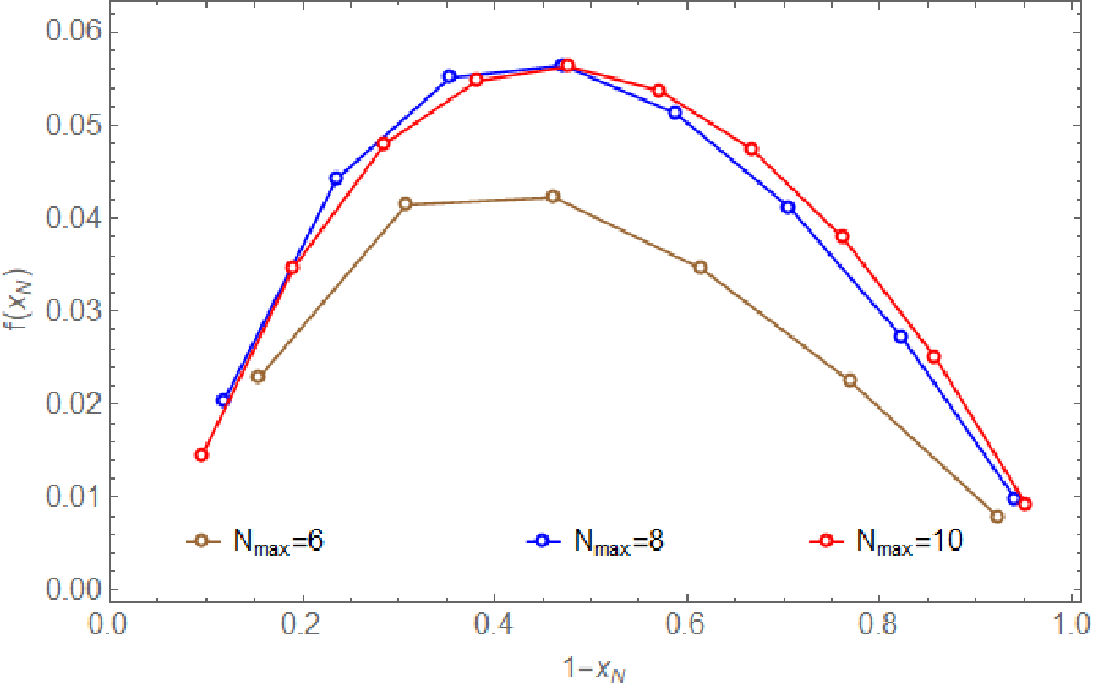
We apply the proton’s LFWF to compute its PDF, which encodes the distribution of the longitudinal momentum carried by its constituents. In this work, such PDF also represents the probability that a proton fluctuates into the constituent nucleon (of the longitudinal momentum fraction $x_{N}$) and pion (of the longitudinal momentum fraction $x_{\pi}$).

In Fig. 2, the proton’s PDF, $f(x_{N})$, is shown as a function of $x_{N}$ and the model space (with parameter settings shown in Table. 1). Note we rescale the the $x$-axis as $x_{\pi}=1-x_{N}$ in the plot. We do not show the results for $f(x_{N}=1)$ in Fig. 2, which represents the probability to find a bare nucleon in the physical proton. For the cases with $N_{\rm max}=$ 6, 8 and 10, such probabilities are 0.83, 0.69, and 0.62, respectively.

For each $N_{\rm max}$, we verified that $f(x_{N})$ satisfies both the normalization condition and the momentum sum rule. As $N_{\rm max}$ increases, $f(x_{N})$ seems to converge (as indicated by the spacing between the curves and the positions of the peaks in the plot). Our results of $f(x_{N})$ peak at about $x_{\pi}=0.45$ (or $x_{N}=0.55$) for the model spaces with $N_{\rm max}=8$ and $10$. In the future, we plan to study $f(x_{N})$ where large/complete model spaces and high Fock sectors are applied. Also, the internal degrees of freedom of the constituents will be included to study the flavor asymmetry of the proton [38, 39, 40, 41].

References

- [1] O. Hen, G. A. Miller, E. Piasetzky and L. B. Weinstein, Rev. Mod. Phys. 89, no. 4, 045002 (2017).
- [2] J. J. Aubert et al. [European Muon Collaboration], Phys. Lett. 123B, 275 (1983).
- [3] H. Cheng and T. Wu, Expanding Protons: Scattering at High Energies (MIT Press, Cambridge, 1987).
- [4] J. P. Vary, H. Honkanen, Jun Li, P. Maris, S. J. Brodsky, A. Harindranath, G. F. de Teramond, P. Sternberg, E. G. Ng and C. Yang, Phys. Rev. C 81, 035205 (2010).
- [5] H. Honkanen, P. Maris, J. P. Vary and S. J. Brodsky, Phys. Rev. Lett. 106, 061603 (2011).
- [6] X. Zhao, H. Honkanen, P. Maris, J. P. Vary and S. J. Brodsky, Phys. Lett. B 737, 65 (2014).
- [7] P. Wiecki, Y. Li, X. Zhao, P. Maris and J. P. Vary, Phys. Rev. D 91, no. 10, 105009 (2015).
- [8] J. P. Vary, L. Adhikari, G. Chen, S. Jia, M. Li, Y. Li, P. Maris, W. Qian, J. R. Spence, S. Tang, K. Tuchin, A. Yu and X. Zhao, Few Body Syst. 59, no. 4, 56 (2018).
- [9] Y. Li, P. Maris, X. Zhao and J. P. Vary, Phys. Lett. B 758, 118 (2016).
- [10] Y. Li, P. Maris and J. P. Vary, Phys. Rev. D 96, no. 1, 016022 (2017).
- [11] S. Tang, Y. Li, P. Maris and J. P. Vary, Phys. Rev. D 98, no. 11, 114038 (2018).
- [12] M. Li, Y. Li, P. Maris and J. P. Vary, Phys. Rev. D 98, no. 3, 034024 (2018).
- [13] S. Jia and J. P. Vary, Phys. Rev. C 99, no. 3, 035206 (2019).
- [14] J. Lan, C. Mondal, S. Jia, X. Zhao and J. P. Vary, Phys. Rev. Lett. 122, no. 17, 172001 (2019).
- [15] X. Zhao, A. Ilderton, P. Maris and J. P. Vary, Phys. Rev. D 88, 065014 (2013).
- [16] X. Zhao, A. Ilderton, P. Maris and J. P. Vary, Phys. Lett. B 726, 856 (2013).
- [17] G. Chen, X. Zhao, Y. Li, K. Tuchin and J. P. Vary, Phys. Rev. D 95, no. 9, 096012 (2017).
- [18] G. A. Miller, Phys. Rev. C 56, 2789 (1997).
- [19] G. A. Miller, Prog. Part. Nucl. Phys. 45, 83 (2000).
- [20] A. Harindranath, Saha Institute of Nuclear Physics, 2005 (unpublished).
- [21] N. A. Tsirova, V. A. Karmanov and J.-F. Mathiot, Phys. Atom. Nucl. 73, 1952 (2010).
- [22] J.-F. Mathiot and N. A. Tsirova, Phys. Atom. Nucl. 76, 1387 (2013).
- [23] C. R. Ji, W. Melnitchouk and A. W. Thomas, Phys. Rev. D 80, 054018 (2009).
- [24] C. R. Ji, W. Melnitchouk and A. W. Thomas, Phys. Rev. D 88, no. 7, 076005 (2013).
- [25] P. Chang and F. Gürsey, Phys. Rev. 164, 1752 (1967).
- [26] S. J. Brodsky, H. C. Pauli and S. S. Pinsky, Phys. Rept. 301, 299 (1998).
- [27] P. Maris, P. Wiecki, Y. Li, X. Zhao and J. P. Vary, Acta Phys. Polon. Supp. 6, 321 (2013).
- [28] K. Hornbostel, S. J. Brodsky and H. C. Pauli, Phys. Rev. D 41, 3814 (1990).
- [29] B. R. Barrett, P. Navratil and J. P. Vary, Prog. Part. Nucl. Phys. 69, 131 (2013).
- [30] M. A. Caprio, P. Maris and J. P. Vary, Phys. Rev. C 86, 034312 (2012).
- [31] H. J. Lipkin, Phys. Rev. 109, 2071 (1958).
- [32] D. H. Gloeckner and R. D. Lawson, Phys. Lett. 53B, 313 (1974).
- [33] J. R. Hiller and S. J. Brodsky, Phys. Rev. D 59, 016006 (1999).
- [34] V. A. Karmanov, J.-F. Mathiot and A. V. Smirnov, Phys. Rev. D 77, 085028 (2008).
- [35] V. A. Karmanov, J.-F. Mathiot and A. V. Smirnov, Phys. Rev. D 82, 056010 (2010).
- [36] V. A. Karmanov, J.-F. Mathiot and A. V. Smirnov, Phys. Rev. D 86, 085006 (2012).
- [37] J. M. Alarcón, D. W. Higinbotham, C. Weiss and Z. Ye, Phys. Rev. C 99, no. 4, 044303 (2019).
- [38] C. A. Aidala et al. [SeaQuest Collaboration], arXiv:1706.09990 [physics.ins-det].
- [39] R. S. Towell et al. [NuSea Collaboration], Phys. Rev. D 64, 052002 (2001).
- [40] E. A. Hawker et al. [NuSea Collaboration], Phys. Rev. Lett. 80, 3715 (1998).
- [41] M. Alberg and G. A. Miller, arXiv:1712.05814 [nucl-th].
- [42] D. R. Entem and R. Machleidt, Phys. Rev. C 68, 041001 (2003).
- [43] E. Epelbaum, H. W. Hammer and U. G. Meissner, Rev. Mod. Phys. 81, 1773 (2009).
- [44] Y. Li, V. A. Karmanov, P. Maris and J. P. Vary, Few Body Syst. 56, no. 6-9, 495 (2015).
- [45] Y. Li, V. A. Karmanov, P. Maris and J. P. Vary, Phys. Lett. B 748, 278 (2015).
- [46] J. P. Vary, R. Basili, W. Du, M. Lockner, P. Maris, D. Oryspayev, S. Pal, S. Sarker, H. M. Aktulga, E. Ng, M. Shao and C. Yang, Proceedings of the International Conference ‘Nuclear Theory in the Supercomputing Era-2016’ (NTSE-2016), Khabarovsk, Russia, September 19-23, 2016. Eds. A. M. Shirokov and A. I. Mazur. Pacific National University, Khabarovsk, Russia, 2018, p. 15. arXiv: 1803.04101.