Clouds of Fluffy Aggregates: How They Form in Exoplanetary Atmospheres and Influence Transmission SpectraTEA (Blecic et al. 2016), TIPS (Gamache et al. 2017), Matplotlib (Hunter 2007)
Abstract
Transmission spectrum surveys have suggested the ubiquity of high-altitude clouds in exoplanetary atmospheres. Theoretical studies have investigated the formation processes of the high-altitude clouds; however, cloud particles have been commonly approximated as compact spheres, which is not always true for solid mineral particles that likely constitute exoplanetary clouds. Here, we investigate how the porosity of cloud particles evolve in exoplanetary atmospheres and influence the cloud vertical profiles. We first construct a porosity evolution model that takes into account the fractal aggregation and the compression of cloud particle aggregates. Using a cloud microphysical model coupled with the porosity model, we demonstrate that the particle internal density can significantly decrease during the cloud formation. As a result, fluffy-aggregate clouds ascend to altitude much higher than that for compact-sphere clouds assumed so far. We also examine how the fluffy-aggregate clouds affect transmission spectra. We find that the clouds largely obscure the molecular features and produce a spectral slope originated by the scattering properties of aggregates. Finally, we compare the synthetic spectra with the observations of GJ1214 b and find that its flat spectrum could be explained if the atmospheric metallicity is sufficiently high ( solar) and the monomer size is sufficiently small (). The high-metallicity atmosphere may offer the clues to explore the gas accretion processes onto past GJ1214b.
Keywords:
planets and satellites: atmospheres — planets and satellites: composition — planets and satellites: individual(GJ1214 b)I Introduction
Transmission spectroscopy is a powerful approach to probe the compositions of exoplanetary atmospheres (Seager & Sasselov 2000; Brown 2001, e.g.,). Recent surveys of transmission spectra have shown that clouds and/or hazes are ubiquitous in exoplanetary atmospheres (Bean et al. 2010; Narita et al. 2013a; Narita et al. 2013b; Kreidberg et al. 2014; Kreidberg et al. 2018; Knutson et al. 2014a; Knutson et al. 2014b; Sing et al. 2016; Crossfield & Kreidberg 2017; Lothringer et al. 2018; Espinoza et al. 2019; Benneke et al. 2019, e.g.,). A remarkable feature of the exoplanet clouds/hazes is that some of them are present at extremely high altitude. For example, the Neptune-sized exoplanet GJ436b and super-Earth GJ1214b are suggested to have an opaque cloud/haze at an altitude as high as – (Knutson et al. 2014a; Kreidberg et al. 2014). The presence of the high-altitude clouds/hazes are also suggested for many hot Jupiters (Sing et al. 2016; Barstow et al. 2017, e.g.,). Understanding how the high-altitude clouds/hazes form may enable us to infer what composition the atmosphere beneath the clouds would have, which in turn might tell us how the planets formed.
In hot, close-in transiting planets, clouds made of condensed minerals potentially form (Morley et al. 2012), and several studies have investigated their formation processes using 1D cloud microphysical models (Helling et al. 2008; Helling et al. 2017; Helling et al. 2019; Lee et al. 2015; Ohno & Okuzumi 2018; Powell et al. 2018; Gao & Benneke 2018; Ormel & Min 2019, e.g.,) as well as 3D models (Lee et al. 2016; Lines et al. 2018; Lines et al. 2019; Roman & Rauscher 2019, e.g.,). Nevertheless, it is still highly uncertain how the high-altitude clouds are formed. Morley et al. 2013; Morley et al. 2015 and Charnay et al. 2015a; Charnay et al. 2015b showed that a high-altitude cloud producing the flat transmission spectrum of GJ1214 b could be formed if the sedimentation velocity of the particles constituting the cloud is sufficiently slow. Recently, Ohno & Okuzumi 2018 modeled the formation of clouds in GJ1214 b and GJ436 by explicitly calculating the size and settling velocity of cloud particles from the microphysics of particle growth. They found that the cloud particles grow too large to ascend to a height of , needed to explain the transmission spectrum of GJ1214 b. Gao & Benneke 2018 also attempted to reproduce the cloud structure of GJ1214 b using a microphysical model that fully solves the evolution of size distribution. However, they concluded the high-altitude cloud of GJ1214 b can only be explained when the eddy diffusion coefficient in the atmospheres is assumed to be at least an order of magnitude higher than predicted from the general circulation model (GCM) with passive tracers (Charnay et al. 2015a). Photochemical hazes may explain the observed spectra if the haze production rate is high enough (Morley et al. 2015; Kawashima & Ikoma 2018; Adams et al. 2019; Lavvas et al. 2019). However, the haze production rate in exoplanetary atmospheres is still highly uncertain, and further laboratory studies (Hörst et al. 2018; He et al. 2018a; He et al. 2018b, e.g.,) are needed to draw robust conclusions.
In this study, we propose that the high-altitude cloud might be the consequence of the porosity evolution of cloud particles. Previous studies commonly assumed that the cloud particle is a compact sphere, but this is not always true for solid condensate particles, as known from the presence of snowflakes in terrestrial atmosphere. Theoretical and experimental studies have suggested that solid particles grow into fluffy aggregates with very low internal density (Dominik & Tielens 1997; Blum & Wurm 2000; Wada et al. 2008, e.g.,). Because the fluffy aggregate has a sedimentation velocity much lower than the compact sphere with same mass, it would easily ascend to the high altitude. Some previous studies pointed out the importance of particle porosity on the vertical structures of mineral clouds (Marley et al. 2013; Ohno & Okuzumi 2018). The effect of porosity evolution was recently studied for photochemical haze formation (Adams et al. 2019; Lavvas et al. 2019), while quantitative investigations have not been carried out yet for mineral cloud formation.
In this paper, we investigate how the porosity of cloud particles evolve in exoplanetary atmospheres, and how it affects the vertical profiles of mineral clouds. Using a cloud microphysical model coupled with the porosity evolution model, we will demonstrate that cloud particle aggregates (CPAs, hereafter) grow without compression in most cases studied here. We will also compute synthetic transmission spectra to study how the fluffy-aggregate clouds influence the observable transmission spectra. The organization of this paper is as follows. We introduce how internal density of an aggregate varies with microphysical processes and establish a porosity evolution model for CPAs in Section II. We describe our microphsical model and investigate the vertical structures of the fluffy-aggregate clouds in Section III. We present the synthetic transmission spectrum and compare it with the observations of GJ1214 b in Section IV. We discuss the caveats of this study and future prospects in Section V. We summarize this paper in Section VI
II Modeling the Formation of Fluffy Aggregates in Mineral Clouds
Fluffy aggregates form through the mutual sticking of solid particles with a low collision energy (Meakin 1991, e.g.,). The smallest particles constituting an aggregate are called monomers. One of the most important quantities that characterize a porous aggregate is the filling factor defined by
| (1) |
where is the mean internal density of the aggregate and are the bulk density of the individual monomers. For aggregates made of single-sized monomers, Equation (1) can also be written as
| (2) |
where is the number of the constituent monomers, and and are the volumes of the aggregate and individual monomers, respectively. Here, the volume of an aggregate is defined as that of a sphere with the same gyration radius. The number of constituent monomers is another important parameter for aggregate of monodisperse monomers because it is directly related to the aggregate mass.
The set of and defines the characteristic size, or length scale, of a porous aggregate. If we approximate an aggregate with a sphere of radius , the ratio of volumes to is , where is the monomer radius. Using this expression with Equation (2), we obtain the relation that determines as a function of and ,
| (3) |
In atmospheres, the filling factor of an aggregate can change through various processes, and we introduce them in following subsections.
II.1 Evolution of the Filling Factor
We introduce how the filling factor of an aggregate evolves via various processes. For convention, we describe a filling factor determined by a specific process using a subscript ; for example, for the collisional compression.
II.1.1 Fractal Growth
Aggregates forming through low-energy sticking collisions often have an open structure with fractal geometry (Meakin 1991, e.g.,). A fractal aggregate can be characterized by the fractal dimension defined by
| (4) |
where is a prefactor of order unity, is the radius of individual monomers, and is the characteristic radius of an aggregate. An aggregate with is “chain-like” in the sense that its length scale is proportional to its mass (), while an aggregate with is “plane-like” in the sense that its cross section is proportional to its mass. Experimental and numerical studies show that aggregates growing by accreting similar-sized aggregates have –, whereas aggregates growing by accreting individual monomers tend to have (Meakin 1991; Okuzumi et al. 2009, e.g.,). Non-ballistic collisions and rotation of aggregates could also reduce the fractal dimension down to (Paszun & Dominik 2006). is often assumed in the studies of haze formation on Titan and Pluto (Lavvas et al. 2010; Gao et al. 2017b, e.g.,). Unless otherwise noted, we assume that aggregate-aggregate collisions dominate over aggregate-monomer collisions, adopting and (Okuzumi et al. 2009). We will discuss the validity of the assumption in Section V.
Once the fractal dimension is given, the filling factor of a fractal aggregate, , can be calculated as a function of . Substituting along with and into Equation (3) and solving for , we obtain
| (5) |
which indicates that the filling factor decreases with increasing , i.e., as the aggregate grows. Whenever two aggregates stick at a low velocity, the newly formed aggregate contains a large void whose volume is comparable to the volume of the collided aggregates (see Section 4 of Okuzumi et al. 2009 for more quantitative analysis). This causes the decrease of the filling factor.
II.1.2 Collisional Compression
The fractal growth described by Equation (5) breaks down if the impact energy is higher than needed for internal restructuring of the newly forming aggregate, for which case collisional compaction occurs (Dominik & Tielens 1997; Blum & Wurm 2000; Wada et al. 2007; Wada et al. 2008; Paszun & Dominik 2009, e.g.,). For a collision between two aggregates with similar individual masses , the collisional energy can approximately be written as
| (6) |
where is the collisional velocity. Here, stands for the mass of the newly forming aggregate, and we have used that the reduced mass of the collided aggregates is . Restructuring of the new aggregate occurs if is much higher than the energy needed to roll one monomer over another monomer in contact by against rolling friction (Dominik & Tielens 1997; Blum & Wurm 2000). Following Dominik & Tielens 1995, we evaluate as
| (7) |
where is the surface energy of the monomers and is the critical rolling displacement above which inelastic rolling occurs. A realistic value of is somewhat uncertain: the model of Dominik & Tielens 1995 anticipates , whereas the measurement by Heim et al. 1999 of the rolling friction force acting on silica microspheres suggests a times larger value. We set to examine maximal impacts of the compression processes.
The filling factor of grain aggregates after collisional internal restructuring has been extensively studied by means of -body dynamical simulations (Wada et al. 2007; Wada et al. 2008; Paszun & Dominik 2009; Suyama et al. 2008; Suyama et al. 2012). According to Wada et al. 2008, the size of an aggregate after a high-energy () collision between two equal-sized fractal () aggregates follows
| (8) |
Using Equation (3), Equation (8) translates into the filling factor after a high-energy collision,
| (9) |
Here, the prefactor corresponds to the filling factor without collisional compression (see Equation 5), whereas the factor represents compression occurring for . Wada et al. 2008 derived Equation (8) for aggregates after a single compressive collision, but Suyama et al. 2008 later confirmed that the expression approximately holds for aggregates growing through multiple compressive collisions (see their Equation (33)).
For particles in atmospheres, the collision velocity in Equation (6) is calculated as the root sum square of the thermal (Brownian) relative velocity and the relative velocity of gravitational settling, i.e.,
| (10) |
Here we write , where is the terminal settling velocity of individual aggregates before collision and is a numerical factor arising from finite width of actual size distribution of the aggregates. We here adopt following Sato et al. 2016. For the terminal velocity of aggregates, we use an expression for spheres (Ohno & Okuzumi 2017),
| (11) |
where and are the characteristic radius and density of aggregates before collision, respectively, is the dynamic viscosity of ambient gas, and is the slip correction factor accounting for the free-molecular flow regime. In Equation (11), we have approximated the aerodynamic radius of an aggregate with its characteristic radius defined by Equation (3). This approximation is invalid for very fluffy aggregates with , for which the aerodynamic radius is generally smaller than the characteristic radius 11 1 The reason can be easily understood for the special case of the free molecular regime, for which the aerodynamic cross section is approximately equal to the projected area (Blum et al. 1996). For , the projected area increases linearly with mass (Minato et al. 2006, e.g.,), but the “characteristic” cross section increases faster than mass (). For , the characteristic cross section is only times larger than the projected area (Okuzumi et al. 2009, see, e.g., Figure 8 of), and therefore the characteristic radius differs from the aerodynamic radius only by . The approximation is even better for (Okuzumi et al. 2009). (Okuzumi 2009). We use this assumption because we only consider in this study. The slip correction factor is given by (Seinfeld & Pandis 2012, e.g.,)
| (12) |
where is the mean free path of gas molecules. The second term in the bracket in Equation (11) corrects for high Reynolds (turbulent) flow, although it is mostly negligible for slowly settling aggregates considered in this study.
II.1.3 Gas-drag Compression
An aggregate moving relative to the surrounding gas can experience compression when the gas drag force acting on it is strong enough to cause internal restructuring. We employ the model of Kataoka et al. 2013b to evaluate the filling factor of an aggregate under gas-drag compression (see Kataoka et al. 2013b; Arakawa & Nakamoto 2016 for applications of the model to dust evolution in protoplanetary disks). We assume that compression occurs when the ram pressure of the gas flow exceeds the static compressional strength of the aggregate. The compression thus proceeds until becomes equal to . Based on the results of -body simulations, Kataoka et al. 2013b found that the static compressional strength can be written as
| (13) |
where is the rolling energy already introduced in Section II.1.2. The ram pressure can be evaluated as the drag force per cross section of the aggregate. For an aggregate setting in an atmosphere at a terminal velocity, the drag force is equal to the gravity , where is the gravitational acceleration. Thus, is given by
| (14) |
Solving together with Equation (3) for , the equilibrium filling factor under gas-drag compression is obtained as
| (15) |
Equation (15) indicates that under gas-drag compression, the filling factor increases with aggregate mass. It is worth noting that is independent of the ambient gas density because the gas drag force balances with the gravity, which does not depend on the gas density.
II.1.4 A General Formula
For a given number of monomers, equivalent to the aggregate mass, one can calculate the equilibrium filling factor from the highest one determined by the fractal growth, gas-drag compression, and collisional compression (Kataoka et al. 2013a), i.e.,
| (16) |
II.2 An Example: KCl Cloud Aggregates in GJ1214b
We here illustrate how the filling factor of CPAs in an super-Earth atmosphere evolves as they grow. We consider the cloud of KCl solid particles in the super-Earth GJ1214b. It is assumed that the cloud has its base at and , where is the atmospheric pressure. The material density and surface energy are and for KCl crystals (Westwood & Hitch 1963). We note that one cannot calculate the filling factor for collisional compression without a knowledge of filling factor of the aggregates before the collision, as the terminal velocity depends on the aggregate density (see Equation 11). Thus, we first calculate only from and , and then is calculated with the obtained .
We find that the internal density of CPAs can be lower than the material density by several orders of magnitude. The evolution pathways of the equilibrium filling factor for , 0.1, and 1 are shown in Figure 1. Here the equilibrium filling factor is expressed as a function of the number of monomers making up the aggregates, . One can see that the aggregates are highly porous, with , over a wide range of . For small , both gas-drag and collisional compression are negligible and the filling factor is determined by fractal growth. Once an aggregate size exceeds a certain value, either collisional or gas-drag compression sets in. For all monomer sizes shown in Figure 1 (–), gas-drag compression always dominates over collision compression. Collisional compression is important for larger monomer sizes and occurs only for around at the cloud base. No matter which compression mechanism dominates, the filling factor increases with , and hence with aggregates mass. Nevertheless, the filling factor never exceeds 0.1 as long as the monomer mass is in the range . The results thus demonstrate the importance of considering the porosity of mineral cloud aggregates.
II.3 Analytic Estimates of Compression Threshold Sizes
To further elaborate how the porosity of CPAs evolve in general cases, we here analytically estimate the threshold sizes at which the compression sets in.
II.3.1 Gas-drag Compression Threshold
Comparison between Equations (5) and (15) shows that exceeds when the number of monomers satisfies
| (17) |
where we use Equation (7). Since for , we find that a aggregate starts to experience gas-drag compression when its characteristic radius exceeds a threshold
| (18) | |||||
It is worth noting that is independent of the monomer size and only depends on material properties and planetary gravity. Equation (18) indicates that gas-drag compression is responsible to aggregates larger than tens micron, while it will be responsible to micron-sized aggregates on high-gravity objects, such as brown dwarfs.
II.3.2 Collisional Compression Threshold
We here estimate the threshold size at which fractal aggregates begin to be compressed by high-energy collisions. Since the thermal kinetic energy is generally several orders of magnitude smaller than the rolling energy , one can consider that only relative velocity from gravitational settling induces collisional compression. For small fractal aggregates, the second term in the bracket in Equation (11) is negligible, and thus we approximately have
| (19) |
For fractal aggregates of , we also have , , and , where is the radius of the newly formed aggregate. Substituting with these expressions into Equation (6), the collisional energy of a settling-induced collision is given by
| (20) |
Collisional compression occurs () when (see Equations (5) and (9)). For (), the threshold size for collisional compression is given by
| (21) | |||||
where we have used the dynamic viscosity for hydrogen-rich atmospheres (Woitke & Helling 2003). In the opposite limit of , for which , we obtain the threshold size of
| (22) | |||||
Here, we have used and , where is the mean thermal velocity of gas molecules and is the mass of a gas molecule.
III Vertical Structure of Fluffy-Aggregate Clouds
III.1 Model
To demonstrate how the porosity evolution affects the cloud structures, we calculate the vertical transport and growth of cloud particles using the double-moment bulk scheme described by Ohno & Okuzumi 2018. The model adopts a 1D Eulerian framework and calculates the vertical distributions of the mass density () and number density () of the cloud particles. The model assumes that the mass distribution of particles is narrowly peaked at the characteristic mass dominating the total cloud mass. In this context, the mass and number densities are related as .
III.1.1 Prescription of Nucleation and Condensation
Formation of the fluffy-aggregate cloud will be triggered by the formation of monomers via nucleation followed by condensation (Figure 2). The processes will determine the size of monomers, which predominantly control the porosity evolution and thus the particle growth. However, microphysical processes associated to the monomer formation—especially the nucleation of initial condensates—are highly uncertain for exoplanetary atmospheres. Although the classical nucleation theory is available, as used in previous studies (Helling & Fomins 2013; Powell et al. 2018; Gao & Benneke 2018, e.g.,), one should keep in mind that the theory sometimes deviates from the nucleation rate measured by numerical and laboratory experiments by several orders of magnitudes (Ford 1997; Tanaka et al. 2011; Lee et al. 2018, e.g.,).
In this study, we mimic the monomer formation by setting the size of monomers as a free parameter. For the sake of simplicity, every monomer is assumed to have the same size. We assume that the nucleation predominantly occurs at the cloud base, and the formed condensate particles instantaneously grow until all condensable vapor at the cloud base is incorporate into the particles. In other words, we calculate the growth of cloud particles in the region above which the monomer formation is completed (Figure 2).
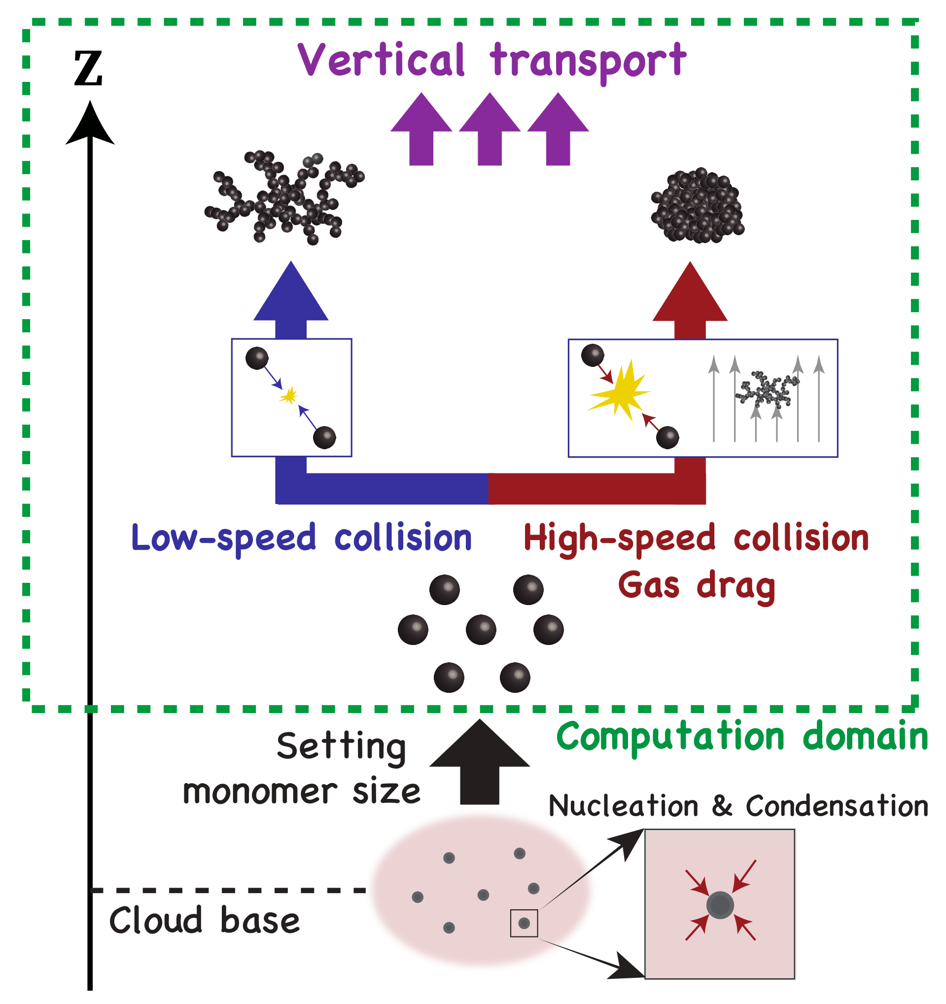
III.1.2 Aggregate Growth and Transport above the Cloud Base
The formed monomers are collided each other and grow into the fluffy aggregates (Figure 2). The aggregates are then mixed in the vertical direction by atmospheric circulation, which we approximate as a diffusion process in the horizontal averaged sense (Parmentier et al. 2013; Charnay et al. 2015a; Zhang & Showman 2018a; Zhang & Showman 2018b). The upward transport is limited by the downward settling motion of the particles. We treat these processes using 1D vertical transport equations with a collisional growth term (Ohno & Okuzumi 2018),
| (23) |
| (24) |
where is the atmospheric gas number density and is the decrease of the aggregate number density due to collisional growth. We use the eddy diffusion coefficient for GJ1214b derived by Charnay et al. 2015a:
| (25) |
where is the eddy diffusion coefficient at depending on the atmospheric metallicity, as listed in Table 1.
Collisional growth is induced by Brownian motion (coagulation hereafter) and differential gravitational settling (coalescence hereafter). We write as
| (26) |
where the first and second terms represent the contribution from coagulation and coalescence, respectively. One can apply the same formula of collisional growth terms for spheres to aggregates by using the characteristic radius of aggregates (Gao et al. 2017a, e.g.,). Approximating an aggregate with a sphere of characteristic radius , the two terms can be written as (Rossow 1978, e.g.,)
| (27) |
and
| (28) |
where is the numerical factor already introduced in Section II.2 and is the collection efficiency originated from the fact that an aggregate strongly coupled to the ambient gas cannot collide with another aggregate. We use the expression (Guillot et al. 2014)
| (29) |
where is the Stokes number.
III.1.3 Numerical Procedures
We consider that the cloud particles are in solid form and made of pure KCl, which is a major condensable species formed in warm (–) exoplanets (Morley et al. 2013; Lee et al. 2018). For super-Earths, the pressure and temperature at cloud forming region (Gao & Benneke 2018, and , see e.g.,) are well below the triple-point pressure and temperature of KCl (Rodrigues & Silva Fernandes 2007, and ,). Thus, the KCl clouds are likely made of solid particles that could grow into an aggregate. We suppose a hypothetical planet that has the PT profile and surface gravity () of GJ1214b. The PT profile is calculated by an analytical model of Guillot 2010 for cloud-free atmospheres as applied in Ohno & Okuzumi 2018, but we additionally include the effect of the convective adjustment by setting the adiabatic lapse late as an upper limit of a temperature gradient.
To obtain the vertical profiles of and , we solve Equations (24) and (23) until the system reaches a steady state. The sizes of aggregates are calculated by using the equilibrium filling factor from Equation (16) at each time step. We note that the collisional compression should occur only when the particle collisions dominate over the vertical transport. Otherwise, the compression can occur without collision, which is clearly unrealistic. To take into account it, we switch off the collisional compression if the vertical mixing timescale is shorter than the collisional growth timescale . The upper boundary condition is set to zero-flux, while the flux at the lower boundary is calculated assuming that and are constant at the cloud base. Since we have assumed that all condensable vapor is incorporated in the cloud particles at the cloud base (Section III.1.1), the cloud mass density at the lower boundary is given by
| (30) |
where is the cloud-base height in pressure and is the saturation vapor density of KCl, which is calculated by the saturation vapor pressure described in Morley et al. 2012. For a given monomer radius, the number density of cloud particles at the lower boundary is also calculated as
| (31) |
The top and bottom of the computation domain are imposed at and the cloud-base height, which is determined by the volume mixing ratio of KCl vapor listed in Table 1 and the saturation vapor pressure. The vertically coordinate is discretized into linearly spaced bins, depending on the atmospheric metallicity (Table 1). The time increment is calculated at each time step so that the fractional decrease of does not exceed , i.e., .
| metallicity | (mol/mol) | (km) | ||
|---|---|---|---|---|
| 1solar | 2.3 | 1.83 | 20 | |
| 10solar | 2.5 | 1.80 | 20 | |
| 100solar | 4.3 | 1.70 | 10 | |
| 1000solar | 16.7 | 1.20 | 5 |
III.2 Results
We here demonstrate how the porosity evolution affects the vertical profiles of KCl clouds. Figure 3 shows the vertical distribution of the size , cloud mass mixing ratio , and filling factor of aggregates for various monomer sizes and atmospheric metallicities. We also plot the vertical profiles of compact () sphere clouds for comparison. The left panels of Figure 3 show that the cloud particles produced at the cloud base grow locally until the timescale of collisional growth becomes comparable to the vertical diffusion timescale. Well above the cloud base, no appreciable growth occurs because the growth timescale increases with height (Ohno & Okuzumi 2018; Powell et al. 2018; Gao & Benneke 2018). Notably, the cloud mass mixing ratio for submicron monomer cases is high even at a very high altitude of as compared to the case of compact-sphere clouds. The reason for this will be explained in a later part of this section.
We note that the aggregate sizes in upper atmospheres may decrease with height in reality, as seen in other studies (Gao & Benneke 2018; Ormel & Min 2019). The trend is not captured in our calculations where the particle sizes are constant at upper atmospheres. This is caused by the fact that our model assumes a narrowly-peaked size distribution that cannot handle the decrease of the mean size caused by the removal of the largest particles from the distribution. However, the size-decreasing effect is presumably not crucial for slowly settling CPAs. This is because the effective size becomes nearly constant in vertical, as seen in our calculations, when the particles have sufficiently small sizes and thus small settling velocity (Gao et al. 2018, see e.g., Figure 4 of).
The trend of vertical size distribution is appreciably different between compact-sphere and fluffy-aggregate cases. For compact-sphere case, the particle size well above the cloud top decreases with decreasing monomer size because a higher number density at the cloud base (which corresponds to a smaller monomer size at the base; see Equation 31) leads to a smaller particle size above the base (Gao et al. 2018; Ohno & Okuzumi 2018; Ormel & Min 2019). The trend is originated from the fact that, for a given mass mixing ratio, a total amount of condensing materials on each particle decreases with increasing a number density. The coagulation is effective for a high number density, but halted once the particle size exceeds the threshold above which the number density becomes too low to cause the collisions (Ohno & Okuzumi 2018, see Section 3.2 of). By contrast, for fluffy-aggregate clouds, the aggregate radius at high altitude increases with decreasing monomer radius . As shown below, this is because the coagulation timescale is a function of aggregate mass and because aggregates made of smaller monomers have to grow to larger in size to obtain a certain mass. For aggregates larger than the mean free path of themselves, the timescale of coagulation growth is approximately given by
| (32) |
which follows from Equation (27). Using the relation , we obtain
| (33) |
which indicates that the coagulation timescale is independent of aggregates properties other than . Since the final size is determined by the balance between coagulation and mixing timescales (), the final aggregate mass is given by
| (34) |
where is the pressure level where the growth is completed. For , the aggregate mass scales as , and hence the final aggregates radius increase with decreasing monomer size.
The aggregate size slightly increase with increasing on atmospheric metallicity. In the case of , for example, the aggregate radii at high altitude are , , , and for the metallicities of , , , and solar abundance, respectively. The increase of the aggregate size is caused by the fact that a higher atmospheric metallicity ( at the cloud base) leads to a higher cloud density that facilitates coagulation growth. This can also be seen from Equation (34), which shows . However, the aggregate size also depends on the mixing timescale (see Equation 34), which decreases with increasing the atmospheric metallicity in our parameter set. This effect substantially cancels out the effects of , which explains the weak metallicity-dependence of the aggregate size in Figure 3.
The key result of this section is that the aggregates never experience compression in the cases studied here. The dot-dashed lines in the left panels of Figure 3 show the threshold size for the gas-drag compression (Equation 18) above which the aggregates leave fractal growth. Figure 3 shows that the particle growth is insufficient to reach the threshold size for the gas-drag compaction. Although the collisional compression can operate on micron-size aggregates in upper atmospheres (, see Equation 22), it does not take place there because the number density is too low to cause the particle collision, i.e., . As a result, aggregates are fractal () even at high altitude.
The absence of the compression enables us to evaluate the vertical extent of clouds. The cloud particle aggregates can ascend to the height of , where is the falling timescales (Charnay et al. 2015a, e.g.,). Assuming for upper atmospheres, the terminal velocity can be approximated as
| (35) |
where we use the relation for . Solving about the pressure, we find the pressure level to which cloud particles can ascend:
| (36) | |||||
where we use . Equation (36) indicates that is independent of the size of cloud particle aggregates . This explains why the cloud particle aggregates made of smaller monomers can ascend higher altitude in Figure 3 despite their very large sizes ().
IV Transmission Spectrum with Fluffy-Aggregate Clouds
The optical properties of fluffy aggregates are considerably different from those of compact spheres. In addition, fluffy aggregates are able to ascend to very high altitude as demonstrated in Section III. In this section, we investigate how these effects influence the transmission spectra of exoplanets.
IV.1 Method
We calculate synthetic transmission spectra of GJ1214b, a super-Earth believed to be covered by clouds (and/or hazes) in very high altitude (Kreidberg et al. 2014, e.g.,), using the vertical profiles of KCl clouds obtained in Section III. We do this by calculating the wavelength-dependent transit depth of a planet, which can be expressed as (Heng & Kitzmann 2017, e.g.,)
| (37) |
where is the reference transit radius and is the optical depth for slant viewing geometry, called the slant optical depth, and is the distance from the center of the planet. We take to be the radius at the pressure level of following previous studies (Kreidberg et al. 2015, e.g.,). The slant optical depth is calculated by integrating the extinction by gas molecules and cloud particles along the observer’s line of sight (Fortney et al. 2003, e.g.,):
| (38) |
where and are the extinction efficiencies of gas molecules and cloud particles, respectively. The stellar radius and planet’s semi-major axis are taken to be and , which are the values for GJ1214b from the Exoplanet eu catalog 22 2 http://exoplanet.eu.
IV.1.1 Gas Opacity
To evaluate the gas opacity, we calculate the mixing ratio of gas molecules using the open-source Thermochemical Equilibrium Abundances (TEA) code (Blecic et al. 2016). The TEA calculates the gas mixing ratio in thermochemical equilibrium for given temperature, pressure, and elemental abundances based on Asplund et al. 2009 using the Gibbs free-energy minimization method. Following Freedman et al. 2008; Freedman et al. 2014, we take into account the molecular absorption of , , , , , , , and as well as the Rayleigh scattering of the molecules. We calculate the absorption and scattering cross sections of the molecules following the method of Kawashima & Ikoma 2018 with the line list of HITRAN2016. The Voigt function is calculated by the polynomial expansion (Kuntz 1997; Ruyten 2004), and the total internal partition function sums are calculated by TIPS code (Gamache et al. 2017). We refer readers to the relevant literature (Rothman et al. 1998; Sharp & Burrows 2007; Malik et al. 2019, e.g.,) for detail methodology of the gas opacity calculations. Further improvements of the line lists and the broadening coefficients (Tennyson & Yurchenko 2018; Gharib-Nezhad & Line 2019, e.g.,) remain for future studies, as our current focus is to study how the fluffy-aggregate clouds influence the transmission spectra.
IV.1.2 Aggregates Opacity
The Mie theory (Bohren & Huffman 1983, e.g.,) is usually used for the calculations of the opacity of spherical particles, but is no longer valid for irregular aggregates. The Mie theory coupled with the effective medium theory is one of the ways to calculate the aggregate opacity (Marley et al. 2013). However, this approach also fails to reproduce scattering properties of an aggregate when the relevant wavelength is much smaller than the aggregate (Tazaki et al. 2016; Tazaki & Tanaka 2018). Aggregates potentially grow to – in size as shown in Section III, while current and future observations mainly use shorter wavelengths such as – for HST/WFC3, – for JWST/NIRSpec (Batalha et al. 2017), and – for ARIEL (Tinetti et al. 2016). Therefore, the effective medium theory is still not a good approximation especially for upcoming observations.
To properly calculate the aggregate opacity, we apply the modified mean field (MMF) theory (Tazaki & Tanaka 2018). The MMF theory is based on the Rayleigh-Gans-Debye (RGD) theory that calculates the interference of single-scattered waves from every monomer by taking the aggregate structure into account (Tazaki et al. 2016) with modifications for multiple scattering within an aggregate using the mean field assumption (Berry & Percival 1986). The MMF theory successfully reproduces the extinction, absorption, and scattering opacities of aggregates calculated by the rigorous T-matrix method in a wide range of wavelength (Tazaki & Tanaka 2018). For calculations, we apply the Gaussian cut-off for the two-points correlation function that specifies the aggregate structure (Tazaki et al. 2016).
Figure 4 shows the extinction opacity of KCl aggregates of for different aggregate sizes and monomer sizes . The refractive index of KCl is taken from Palik 1985 compiled by Kitzmann & Heng 2018. In the examples presented here, the extinction opacity is dominated by scattering in the wavelength range –. At longer wavelengths, absorption dominates over scattering, and the absorption peak of KCl appears at . It is worth noting that the absorption feature is visible even if aggregate size is very large, as seen in the case of . This is because, unless the multiple scattering becomes dominant, the absorption cross section of an aggregate is the sum of the absorption of every monomer, and thus the wavelength dependence is the same as that of an individual monomer (Berry & Percival 1986; Tazaki & Tanaka 2018).
According to the MMF theory, the optical properties of an aggregate behave differently among three wavelength regimes , , and . In the first regime, geometric optics applies to the constituent monomers, and the scattering cross section is approximately given by , independent of wavelength. In the opposite limit of , the Rayleigh limit applies to the aggregate, and the scattering cross section obeys the well-known law . I the left panel of Figure 4, this can be seen in the case of , at –.
The intermediate regime provides unique opacity properties for aggregates. For this regime, we find that the scattering opacity scales with wavelength dependence as (see Figure 4). In this intermediate regime, the scattered wave by an aggregate is a superposition of singly scattered waves from individual monomers, and the scattering cross section of a aggregate has following dependence. (Berry & Percival 1986, Section 5)
| (39) |
where is a constant order of unity. This explains the scattering slope for and in the left panel of Figure 4. The unique scattering slope is caused by interference among the scattered waves from individual monomers. The scattered waves toward large scattering angles () cancel out because of the presence of waves with opposite phases, leading to the dependence (Kataoka et al. 2014).
IV.2 Cloud-top Pressure
Before showing the synthetic spectra, we investigate the cloud-top pressure, defined as the pressure level at which the cloud becomes optically thick along the line of sight of an observer (i.e., ). The cloud-top pressure clarifies the observable region of atmospheres and was examined by previous studies (Ohno & Okuzumi 2018; Powell et al. 2018; Gao & Benneke 2018; Helling et al. 2019). Figure 5 shows the cloud-top pressure of fluffy-aggregate clouds as a function of wavelength for different monomer sizes and the atmospheric metallicities. In general, the cloud top is located at a lower atmosphere for longer wavelength because the scattering opacity decreases with increasing wavelength for (see Figure 4). We note that the cloud top hardly exceeds the altitude of (dashed lines in Figure 5) for parameter ranges examined in this study. In near-infrared wavelength, the cloud-top height increases with decreasing monomer size as long as , as CPAs constituted by smaller monomers ascend to higher altitude. On the other hand, the cloud-top height also decreases with decreasing monomer size for . This opposite trend is caused by the monomer size dependence of aggregate scattering opacity. Using Equation (39) and an aggregate mass , one can see that the scattering mass opacity follows
| (40) |
Thus, the scattering mass opacity decreases with decreasing monomer size. On the other hand, in the limit of small monomer size (i.e., ), the cloud mass mixing ratio is vertically constant and independent of monomer size (see Figure 3). Therefore, the scattering efficiency () and thus the cloud-top height decrease with decreasing monomer size for very small .
We also find that the cloud-top pressure tends to be smaller for higher atmospheric metallicities. This is because the cloud mass mixing ratio increases with increasing the metallicity. Specifically, the cloud-top pressure for the atmospheric metallicity of and solar reach at near-infrared wavelength if the monomer is smaller than . It is worth pointing that the fluffy-aggregate clouds can produce the cloud top at the pressure level comparable to that retrieved from the observations of HST/WFC3 for GJ1214b (Kreidberg et al. 2014), which was hardly attained by the compact-sphere clouds in our previous study (Ohno & Okuzumi 2018).
IV.3 Synthetic Spectra
We begin by studying how the aggregate structure affects transmission spectra. For later convenience, we introduce a metric characterizing the spectral slope, given by (Line & Parmentier 2016, e.g.,)
| (41) |
where is the power-law index of the extinction efficiency of atmosphere, i.e., (. For example, for the Rayleigh scattering particles, and for gray cloud particles. Here, we have naively used the pressure scale height instead of the cloud scale height. Strictly speaking, the the could scale height is equal to only when the particle settling timescale is much longer than the mixing timescale (Ohno & Okuzumi 2018, see e.g., Equation (33) of). The cluod scale height is smaller than at high altitude where the cloud mass mixing ratio decreases with increasing height, implying . However, cloud particles at such very high altitude are usually so depleted that their contribution to transmission spectra is small. In fact, as shown in previous section, the cloud top hardly exceeds the the pressure level of for the parameter space examined in this study. Therefore, Equation (41) offers a reasonable diagnosis of the spectral slope.
Figure 6 shows the synthetic transmission spectra of GJ1214b with a solar-metallicity atmosphere and with a KCl cloud obtained from compact-sphere and fluffy-aggregate models (see the top rows of Figure 3 for the cloud vertical structure). We set the reference radius to so that the cloud-free solar-composition atmosphere produces the planet-to-star radius ratio of (i.e., ) in near-infrared (Narita et al. 2013a, e.g.,). We calculate the optical properties of compact spheres using the Mie theory (Bohren & Huffman 1983, e.g.,). For comparison, we also plot the transmission spectrum for the cloud-free atmosphere, which exhibits molecular absorption signatures of mainly molecules and the spectral slope in caused by the Rayleigh scattering of molecules. In the left panel of Figure 6, the compact-sphere clouds produce a floor of the transit depth at . In the compact-sphere model, a cloud deck that is gray in visible is produced no matter how small the monomers at the cloud base are, because they always grow to in size through coagulation as shown in Section III (see also Ohno & Okuzumi 2018).
The transmission spectrum for fluffy-aggregate clouds exhibit a considerably different shape from that for compact-sphere clouds. Since the fluffy-aggregate cloud is lofted to much higher altitude, the absorption features in the spectra are largely obscured as compared to the cases of the compact-sphere clouds except for the case of in which the effect that decreases the cloud extinction efficiency is important (Section IV.2). Furthermore, the fluffy-aggregate clouds produce a spectral slope at , in particular when the monomers are small. The spectrum for is nearly identical between the fluffy-aggregate and compact-sphere models because the monomers satisfy at near-infrared wavelengths. The spectral slope for and is well characterized by , originated by the wavelength dependence of the scattering opacity for (see Section IV.1.2).
Since the spectral slope with originates from the scattering property of aggregates, it could potentially be used as an observational signature for CPAs when the atmospheric scale height is well constrained. We find that the slope with also emerges for many other materials that may build up mineral clouds on exoplanets (Appendix A). However, caution should be taken regarding this interpretation because may also be caused by the combination of small and large compact spheres.
Although the fluffy aggregates can largely obscure the molecular features in visible to near-infrared, they are optically too thin to hide the features at longer wavelengths (), as can be seen in Figure 7. This implies that future transmission spectroscopy at with JWST and ARIEL could detect molecular features in super-Earths that look cloudy in visible and near-infrared.
The transmission spectrum from the fluffy-aggregate model also substantially depends on the atmospheric metallicity. Figure 7 shows the transmission spectra from the fluffy-aggregate model for various atmospheric metallicities, where is assumed for every case. One can see that the higher the atmospheric metallicity is, the flatter the spectral slope is. This is because the gradient of spectral slope is proportional to the pressure scale height (see Equation 41), which decreases with increasing the atmospheric metallicity. The effect is notable for solar metallicity, and the spectral slope is almost flat for solar metallicity.
IV.4 Comparison with Observations of GJ1214b
Here, we compare our synthetic transmission spectra with the observed transmission spectrum of GJ1214b. We calculate the cloud profiles as well as the synthetic spectra for the atmospheric metallicities of – solar abundances and monomer sizes of –. We also vary the reference radius from to to be consistent with the observed planet radius. The relative goodness-of-fit for each model is quantified by the reduced chi-square . The model freedom is the number of data points minus three, the number of the fitting parameters (atmospheric metallicity, monomer size, and reference radius). For instance, Morley et al. 2015 assumed that an acceptable model for GJ1214b produces if only data points from the HST/WFC3 observations (Kreidberg et al. 2014) are used.
The left panel of Figure 8 shows the best-fit transmission spectra for the metallicity of , , , and solar abundance, compared with the observational data for GJ1214b from HST/WFC3 (Kreidberg et al. 2014) and Spitzer/IRAC (Gillon et al. 2014). All available observational data are also denoted as gray dots in the left panel of Figure 8. The right panel shows the best-fit spectra only for HST/WFC3. For all data points (left panel), the smallest reduced chi-square for the atmospheric metallicities of , , , and solar abundance are , , , and , respectively. However, these values are significantly affected by the large scatter in the data at visible wavelengths. If we only focus on the data point of HST/WFC3 (Kreidberg et al. 2014) and Spitzer/IRAC (Gillon et al. 2014), which are less scattered than the visible data, we obtain the reduced chi-squared of , , , and for the metallicities of , , , and solar abundance, respectively. For a comparison with the HST data only (right panel), the reduced chi-squared values are ,, , and for atmospheric metallicities of , , , and solar abundance, respectively. Overall, a higher atmospheric metallicity leads to a smaller reduced chi-squared value. We also find that the presence of the fluffy-aggregate cloud appreciably improves the goodness-of-fit of the model as compared to the cloud-free case. For the comparison with the HST data as an example, the cloud-free atmosphere with solar metallicity yields (the black line in the right panel of Figure 8), whereas the model with the fluffy-aggregate clouds yields . The reduced chi-square for each parameter set is summarized in Figure 9.
Our results show that the model with a higher atmospheric metallicity yields a better match to the observational data. The high-metallicity atmospheres supply sufficient KCl condensates, and the produced clouds can obscure the molecular features if monomer size is sufficiently small, namely . Indeed, the molecular absorption at around , noticeable in cloud-free atmospheres even with solar metallicity, is significantly weakened by the cloud opacity (right panel of Figure 8). The spectral slope is also closer to the observed flat spectrum because of the relatively small scale height. Notably, the model with solar metallicity yields for the comparisons with Kreidberg et al. 2014, which is comparable to the obtained by Gao & Benneke 2018 who assumed the eddy diffusion coefficient much larger than that predicted by 3D GCM (Charnay et al. 2015a). Our results suggest that it would be able to explain the observed spectra of GJ1214b in the range of predicted by the GCM, if the mineral cloud consist of fluffy aggregates. We emphasize that as the metallicity is increased, the resulting synthetic spectrum better matches the transit depth at mid-infrared wavelengths, especially at , observed by the Spitzer/IRAC (see the left panel of Figure 8). This is thanks to the absorption of whose abundance increases with increasing the atmospheric metallicity (Moses et al. 2013).
There are two reasons why the low-metallicity models ( and solar) fail to match the observations. The first is an insufficient cloud abundance: the mixing ratio of KCl in the low-metallicity atmosphere is too low to produce sufficiently opaque clouds. The second reason is that, more importantly, the spectral slope caused by the aggregate opacity is too steep to match the flat spectrum observed by the HST/WFC3 (Kreidberg et al. 2014) because of the large scale height (see Section IV.3). Therefore, our fluffy-aggregate cloud model still requires a small atmospheric scale height to explain the flat spectrum of GJ1214b, which is achieved by the high-metallicity atmosphere.
Although the fluffy-aggregate clouds potentially explain the featureless spectrum of GJ1214b, we note that the CPAs need to be constituted by monomers with (see Figure 9). The monomer size is presumably controlled by the formation of condensation nuclei, namely the nucleation, and subsequent condensation growth that keeps a spherical shape (Lavvas et al. 2011). If one adopts the classical nucleation theory, the homogeneous nucleation followed by condensation yields KCl particles with the effective size of (Gao & Benneke 2018). This is substantially larger than the required monomer size. This could suggest that classical nucleation theory underestimates the nucleation rate of , because a larger number of condensation nuclei generally leads to a smaller monomer size (Gao et al. 2018; Ohno & Okuzumi 2018). In fact, Lee et al. 2018 reports that classical nucleation theory underestimates the nucleation rate of . Alternatively, a number of stable, small nuclei could be produced by the heterogeneous nucleation of onto (Gao & Benneke 2018), although its nucleation rate depends on the desorption energy of that is currently unknown. Laboratory studies of nucleation and condensation would be important to predict the monomer size in exoplanetary atmospheres, which in turn test the scenario of the fluffy-aggregate cloud for GJ1214b.
V Discussion
V.1 Model Caveats
In this study, we have adopted simplified porosity and microphysical model. The models are useful to clarify the effects of the porosity evolution, but involves some caveats because of its simplicity. In what follows, we state the caveats of our model and discuss their possible impacts on the results.
V.1.1 Validity of for Other Size Distributions
The most strong assumption of our porosity model may be the fractal dimension of for the fractal growth (Section II.1.1). We have adopted this assumption since our cloud microphysical model assumes the narrowly peaked size distribution, for which the equal-sized collision is a dominant growth process. However, the cloud particles could have different shape of size distributions (Powell et al. 2018; Gao & Benneke 2018), and the monomer-aggregate collision might be dominant. In that case, CPAs grow into more spherical shapes (e.g., ), and the cloud vertical extent would be small as compared to the case of .
Here, we test the validity of the assumption for various size distributions. We introduce a mass-weighted collision rate onto a particle with mass (), defined as (Okuzumi 2009)
| (42) |
where is the collision kernel between particles with masses and , and is the number density of particles with masses between and . Equation (42) measures the contributions of aggregates with masses of on the growth of aggregate with mass of . We assume that the cloud particles obey the Hansen size distribution (Hansen 1971), described as
| (43) |
where is the mean effective radius and is the effective variance. The shape of the size distribution is controlled by the effective variance ; for example, yields log-normal-like distributions, while yields power-low-like distributions.
Figure 10 shows the mass-weighted collision rate and size distributions for , , and . We assume and calculated from the mass-weighted particle size:
| (44) |
We use the collision kernel described in Chapter 15 of Jacobson 2005 assuming a constant particle density. Figure 10 demonstrates that the growth is largely contributed by the collisions of particles with masses of –. According to Okuzumi et al. 2009, collisions with mass ratio of – lead to the fractal dimension of – (see their Figure 6), which is almost the same as assumed in this study. Thus, the assumption of may be reasonable for various shapes of size distributions. However, it should be noted that the size distribution of the CPAs has been unknown to date. We will examine how the size and porosity distributions of CPAs evolve in exoplanetary atmospheres in our forthcoming paper.
V.1.2 Limitation of the Compression Model
Here we state several limitations of a compression model adopted in Section II.1.3. First, the relation between mass and size of the collisionally compressed aggregates (Equation 8) was derived for collisions between two equal-mass aggregates with (Wada et al. 2008). For different-mass collisions, the degree of compression is evaluated from the comparison of the impact energy with work done by dynamic compression strength (Suyama et al. 2012). we also note that the head-on-collision is assumed here, but offset collisions could induce the elongation of aggregates, further hinders the compression (Paszun & Dominik 2009). Second, the static compression strength used for the gas-drag compression (Equation 13) was derived for an aggregate whose internal structure is characterized by (Kataoka et al. 2013b). The compression strength for different was recently proposed by Arakawa et al. 2019 from a semi-analytical argument. Although the verification with numerical experiments remain to be carried out, their formula is potentially applicable to our compression model. Further numerical experiments will be helpful to extend the compression model to more universal cases.
V.1.3 Simplified Nucleation and Condensation
In this study, we have assumed that saturated vapor is instantaneously incorporated into the condensation nuclei at the cloud base. This assumption would be reasonable since the condensation timescale is much shorter than the vertical mixing timescale near at the cloud base (Ohno & Okuzumi 2018; Powell et al. 2018; Gao & Benneke 2018). Additional condensation could transform the CPAs to sphere-like particles if the surface growth rate via condensation dominates over the coagulation rate (Lavvas et al. 2011). However, the effect is presumably insignificant for KCl clouds because other condensing species, such as and MnS, have the cloud bases at deeper atmospheres and are likely depleted at the KCl cloud formation region (Mbarek & Kempton 2016, e.g.,). ZnS is an only species whose cloud base is placed near at the KCl cloud base (Morley et al. 2012, e.g.,). But, we expect that CPAs are still present as aggregates even if ZnS condensation takes place. This is because the abundance of ZnS is 2–3 times lower than KCl and likely insufficient to fill all pores.
We have also assumed that the nucleation followed by condensation, namely the monomer formation, occurs right at the cloud base. This would be true if the condensation nuclei are supplied from deep atmospheres, as argued in Lee et al. 2018. On the other hand, the monomer formation could occur above the cloud base in the context of homogeneous nucleation that needs significant supersaturation to set in (Helling & Fomins 2013, e.g.,). The monomers formed in upper atmospheres might increase the of CPAs through different-size collisions. We expect that the resulting is still close to , as discussed in Section V.1.1, though a microphysical model solving size distributions will be needed to verify it.
V.2 Comparison with Other Porosity Models
Some previous studies of haze microphysics adopted a porosity model different from ours (Wolf & Toon 2010; Adams et al. 2019). The porosity model adopted in the haze models assumes that the fractal dimension approaches as the number of monomers increase. The assumed fractal dimension is comparative to that was observed for an aggregates with maximal compression via high-energy collisions in the numerical experiments (Wada et al. 2008; Suyama et al. 2008). However, the threshold at which compression sets in is considerably different from our model. Figure 11 shows the fractal dimension as a function of the number of monomers in Adams et al. 2019 and our model, where we calculate from Equations (3) and (4):
| (45) |
For comparisons, we use the surface energy of tholine (Yu et al. 2017) and material density . In the model of Adams et al. 2019, the fractal dimension increases to at , while our model predicts that the compression sets in –, depending on the monomer size. Thus, the aggregate hazes in previous studies were assumed to be compressed much easier than our prediction. This is presumably a reason why aggregate hazes in Adams et al. 2019 tend to produce flat spectra rather than those with spectral slopes.
The easily compressed aggregates in previous studies were speculated from the laboratory study of soot formation in a flame. In the experiments, it was observed that the soot-aggregates are restructured by the Coulomb interaction between oppositely charged parts (Onischuk et al. 2003). However, one should take a caution about the compression due to the Coulomb interaction because the charge states of aerosols in exoplanetary atmospheres are poorly known. Investigating the aerosol charge processes (Helling et al. 2011a; Helling et al. 2011b, e.g.,) might help to evaluate if the restructuring due to Coulomb interaction is possible.
V.3 Implications for Spectral Slopes of Hot-Jupiters
The presence of mineral clouds has also been suggested for a number of hot-Jupiters (Sing et al. 2016; Barstow et al. 2017, e.g.,). A recent retrieval study by Pinhas et al. 2019 suggested that the hot-Jupiters whose transmission spectra were provided by Sing et al. 2016 typically exhibit transmission spectral slopes of . This is considerably steeper than the slope originated from the aggregate scattering opacity () and even steeper than the Rayleigh slope (). Such “super-Rayleigh” slopes might be produced by the absorption of tiny cloud particles made of sulfide minerals (Pinhas & Madhusudhan 2017). However, we find that CPAs made of sulfide minerals do not produce such steep wavelength dependence (see Figure 12 in Appendix A) unless the aggregate is extremely small. This is because the steep absorption feature of sulfide minerals is largely obscured by the scattering opacity. Thus, it is more likely that the super-Rayleigh slopes of hot-Jupiters are caused by other physical processes than fluffy-aggregate cloud formation, such as NUV absorbers like SH (Evans et al. 2018). Alternatively, the slope potentially implies physical processes that halt the aggregation, leading to a tiny particle size. Electrostatic repulsion (Okuzumi 2009, e.g.,) may be promising because the ionization of alkali metals, likely produces charged cloud particles, takes place at hot-Jupiters (Batygin & Stevenson 2010, e.g.,). We will examine this possibility in future studies.
V.4 Implications for High Metallicity Atmospheres on Planetary Formation
The high-metallicity atmosphere is of interest from the perspective of planetary formation theory. Our results suggest that, if the flat spectrum of GJ1214b is caused by the condensation clouds, high-metallicity atmosphere ( soar) is plausible to explain the observations, as suggested by other studies (Morley et al. 2015; Gao & Benneke 2018). This is in contrast to some other super-Earths or exo-Neptunes that likely retain metal-poor ( soar) atmospheres, such as GJ3470b (Benneke et al. 2019) and HAT-P-26b (Wakeford et al. 2017; MacDonald & Madhusudhan 2019). On the other hand, metal-rich ( soar) atmospheres have also been suggested for some exo-Neptunes, such as GJ436b (Morley et al. 2017) and HAT-P-11b (Fraine et al. 2014). The diversity of the atmospheric metallicity potentially suggests different formation processes of these planets. For example, planets with a low-metallicity atmosphere may have formed from large building blocks, such as protoplanets, that less affect atmospheric composition (Fortney et al. 2013). A high-metallicity atmosphere may suggest that a substantial metal-enrichment of the atmosphere, potentially caused by the accretion of small planetesimals and/or pebbles (Fortney et al. 2013; Lambrechts et al. 2014; Venturini et al. 2016; Venturini & Helled 2017), occurred during the formation of the planet.
The presence of high-metallicity atmospheres poses another interesting question associated to the past formation process: how did the super-Earths avoid to be gas giants? It has been suggested that the high atmospheric metallicity leads to the runnaway gas accretion even for planets with Earth-masses (Hori & Ikoma 2011; Venturini et al. 2015). Thus, the gas accretion must be inhibited in order to form a super-Earth rather than a gas giant. One of the scenario is that they were formed in the late stage of protoplanetary disks where the disk gasses were almost dissipated (Ikoma & Hori 2012; Lee et al. 2014; Lee & Chiang 2016, e.g.,). Alternatively, the high-metallicity atmospheres may suggest the presence of mechanisms regulating the gas accretion, such as the gap formation and weak viscous accretion of disc gasses (Tanigawa & Ikoma 2007; Tanigawa & Tanaka 2016; Ogihara & Hori 2018). Rapid recycling of the atmospheric gas embedded in protoplanetary disc, which is observed in recent hydrodynamical simulations (Ormel et al. 2015; Lambrechts & Lega 2017; Kurokawa & Tanigawa 2018; Kuwahara et al. 2019, e.g.,), also delays the runnaway gas accretion, but it might be difficult to produce the high-metallicity atmosphere unless the disc gas is highly enriched in heavy elements. The evolution of atmospheric composition after the disk dissipation, like that suggested for solar-system terrestrial planets (Sakuraba et al. 2019), might increase the atmospheric metallicity even if the planet originally possessed a low-metallicity atmosphere. Further studies linking the formation processes to the atmospheric metallicity would be warranted to explore the past formation processes of super-Earths with high-metallicity atmospheres.
VI Summary
We have investigated how the porosity of cloud particle aggregates (CPAs) evolve in exoplanetary atmospheres. Based on the results of numerical experiments investigating the aggregate restructuring, we have constructed a porosity evolution model that takes into account the fractal growth, collisional compression, and the compression caused by gas drag. Using a cloud microphysical model coupled with the porosity model, we have examined how the porosity evolution influences the cloud vertical distributions and observed transmission spectra of GJ1214b. Our findings are summarized as follows.
(1) The internal density of CPAs can be much lower than the material density by – orders of magnitudes (Section II), depending on the size of monomers. The gas-drag compression sets in once the CPA becomes larger than (Equation 18). The collisional compression is less important than the gas-drag compression in most cases studied here.
(2) The compression of CPAs hardly occurs during the KCl cloud formation since the particle growth is not sufficient to induce the compression (Section III). Thus, the porosity evolution in general results in the cloud vertical extent much larger than that of the compact-sphere clouds. Without the compression, the fluffy-aggregate clouds can ascend to the height where the monomer can ascend to (Equation 36).
(3) The fluffy-aggregate clouds largely obscure the absorption signatures of gas molecules in transmission spectra because of the large vertical extent if the aggregates are constituted by submicron monomers (Section IV.3). Although the spectra in visible to near-infrared tend to be featureless, the fluffy-aggregate clouds become optically thin at longer wavelength (). Future observations probing mid-infrared wavelength, such as JWST and ARIEL, may be able to detect molecular signatures even if the spectrum looks featureless in visible to near-infrared wavelength.
(4) CPAs also produce the spectral slope originated by the scattering properties of aggregates (Section IV.1.2). The slope reflects the wavelength dependence of the aggregate scattering opacity, (Section IV.3). This could be potentially used as an observable signature of CPAs if the atmospheric scale height is well constrained.
(5) Comparing our synthetic spectra with the observations of GJ1214b, we find that the models of the high-metallicity atmospheres ( solar) well matches the observations if the CPAs are constituted by submicron monomers (Section IV.4). This is due to the fact that the spectral slope produced by CPAs mismatches the observed flat spectrum as long as the atmospheric scale height is large. The predicted high-metallicity atmosphere potentially suggests the presence of mechanisms regulating the gas accretion onto past GJ1214b.
We note that our results do not rule out other scenarios explaining the flat spectrum of GJ1214b, such as photochemical hazes (Morley et al. 2015; Kawashima & Ikoma 2018; Kawashima & Ikoma 2019; Kawashima et al. 2019; Adams et al. 2019; Lavvas et al. 2019). The spectrum with hazes could also match the observations if the haze production rate is sufficiently high (Lavvas et al. 2019). On the other hand, the hazes tend to produce the spectral slope caused by the haze opacity in the Rayleigh regime (Kawashima & Ikoma 2018; Kawashima & Ikoma 2019; Lavvas et al. 2019). Therefore, from the same reason what we discussed for fluffy-aggregate clouds, the high-metallicity atmosphere may be still needed to explain the flat spectrum with photochemical hazes. However, if hazes grow into moderately compressed aggregates (), it could be possible to explain the flat spectrum with solar-metallicity atmosphere (Adams et al. 2019). Exploring the porosity evolution of hazes will be helpful to constrain the atmospheric metallicity of GJ1214b.
The compact-sphere cloud is still not ruled out (Gao & Benneke 2018). for settling aerosols is still uncertain, and there is an order of magnitude uncertainty among different model predictions (Komacek et al. 2019, e.g.,). Although GJ1214b is a close-in planet (semi-major axis is ), it might retain a non-zero eccentricity (Charbonneau et al. 2009; Carter et al. 2011) that yields distinct atmospheric circulations (Kataria et al. 2013; Lewis et al. 2017; Ohno & Zhang 2019, e.g.,) and possibly . If it is possible to distinguish the fluffy-aggregate and compact-sphere clouds from observations, it might help to understand the aerosol transport processes in exoplanetary atmospheres.
Appendix A Aggregate Opacity for Other Mineral Clouds
In this appendix, we show the opacity of an aggregate made of various materials that potentially build up exoplanetary mineral clouds. We have selected a variety of condensable materials (ZnS, , MnS, Cr, , , Fe, ) listed in Morley et al. 2012 and some nucleating species (Helling et al. 2017; Helling et al. 2019, , C, see e.g.,). The refractive indices of the materials are taken from Kitzmann & Heng 2018. Figure 12 summarizes the calculated extinction opacities for and . Some materials exhibit characteristic absorption features at ; for example, for , for , and for . Absorption also dominates over extinction at for all materials. On the other hand, the extinction opacity at – is mostly dominated by scattering. Therefore, many minerals other than KCl also produce an aggregate scattering slope of (Section IV.1.2) at visible to near-infrared wavelengths. The exception we found is graphite, C, whose opacity is dominated by absorption even at near-infrared wavelengths.
References
- Adams et al. (2019) Adams, D., Gao, P., de Pater, I., & Morley, C. V. 2019, ApJ, 874, 61
- Arakawa & Nakamoto (2016) Arakawa, S., & Nakamoto, T. 2016, ApJ, 832, L19
- Arakawa et al. (2019) Arakawa, S., Takemoto, M., & Nakamoto, T. 2019, arXiv e-prints, arXiv:1908.03125
- Asplund et al. (2009) Asplund, M., Grevesse, N., Sauval, A. J., & Scott, P. 2009, ARA&A, 47, 481
- Barstow et al. (2017) Barstow, J. K., Aigrain, S., Irwin, P. G. J., & Sing, D. K. 2017, ApJ, 834, 50
- Batalha et al. (2017) Batalha, N. E., Mandell, A., Pontoppidan, K., et al. 2017, PASP, 129, 064501
- Batygin & Stevenson (2010) Batygin, K., & Stevenson, D. J. 2010, ApJ, 714, L238
- Bean et al. (2010) Bean, J. L., Miller-Ricci Kempton, E., & Homeier, D. 2010, Nature, 468, 669
- Bean et al. (2011) Bean, J. L., Désert, J.-M., Kabath, P., et al. 2011, ApJ, 743, 92
- Benneke et al. (2019) Benneke, B., Knutson, H. A., Lothringer, J., et al. 2019, Nature Astronomy, 361
- Berry & Percival (1986) Berry, M. V., & Percival, I. C. 1986, Optica Acta, 33, 577
- Berta et al. (2012) Berta, Z. K., Charbonneau, D., Désert, J.-M., et al. 2012, ApJ, 747, 35
- Blecic et al. (2016) Blecic, J., Harrington, J., & Bowman, M. O. 2016, ApJS, 225, 4
- Blum & Wurm (2000) Blum, J., & Wurm, G. 2000, Icarus, 143, 138
- Blum et al. (1996) Blum, J., Wurm, G., Kempf, S., & Henning, T. 1996, Icarus, 124, 441
- Bohren & Huffman (1983) Bohren, C. F., & Huffman, D. R. 1983, Absorption and scattering of light by small particles
- Brown (2001) Brown, T. M. 2001, ApJ, 553, 1006
- Carter et al. (2011) Carter, J. A., Winn, J. N., Holman, M. J., et al. 2011, ApJ, 730, 82
- Charbonneau et al. (2009) Charbonneau, D., Berta, Z. K., Irwin, J., et al. 2009, Nature, 462, 891
- Charnay et al. (2015a) Charnay, B., Meadows, V., & Leconte, J. 2015a, ApJ, 813, 15
- Charnay et al. (2015b) Charnay, B., Meadows, V., Misra, A., Leconte, J., & Arney, G. 2015b, ApJ, 813, L1
- Colón & Gaidos (2013) Colón, K. D., & Gaidos, E. 2013, ApJ, 776, 49
- Croll et al. (2011) Croll, B., Albert, L., Jayawardhana, R., et al. 2011, ApJ, 736, 78
- Crossfield & Kreidberg (2017) Crossfield, I. J. M., & Kreidberg, L. 2017, AJ, 154, 261
- de Mooij et al. (2012) de Mooij, E. J. W., Brogi, M., de Kok, R. J., et al. 2012, A&A, 538, A46
- Désert et al. (2011) Désert, J.-M., Bean, J., Miller-Ricci Kempton, E., et al. 2011, ApJ, 731, L40
- Dominik & Tielens (1995) Dominik, C., & Tielens, A. G. G. M. 1995, Philosophical Magazine, Part A, 72, 783
- Dominik & Tielens (1997) —. 1997, ApJ, 480, 647
- Espinoza et al. (2019) Espinoza, N., Rackham, B. V., Jordán, A., et al. 2019, MNRAS, 482, 2065
- Evans et al. (2018) Evans, T. M., Sing, D. K., Goyal, J. M., et al. 2018, AJ, 156, 283
- Ford (1997) Ford, I. J. 1997, Phys. Rev. E, 56, 5615
- Fortney et al. (2013) Fortney, J. J., Mordasini, C., Nettelmann, N., et al. 2013, ApJ, 775, 80
- Fortney et al. (2003) Fortney, J. J., Sudarsky, D., Hubeny, I., et al. 2003, ApJ, 589, 615
- Fraine et al. (2014) Fraine, J., Deming, D., Benneke, B., et al. 2014, Nature, 513, 526
- Fraine et al. (2013) Fraine, J. D., Deming, D., Gillon, M., et al. 2013, ApJ, 765, 127
- Freedman et al. (2014) Freedman, R. S., Lustig-Yaeger, J., Fortney, J. J., et al. 2014, ApJS, 214, 25
- Freedman et al. (2008) Freedman, R. S., Marley, M. S., & Lodders, K. 2008, ApJS, 174, 504
- Gamache et al. (2017) Gamache, R. R., Roller, C., Lopes, E., et al. 2017, Journal of Quantitative Spectroscopy and Radiative Transfer, 203, 70
- Gao & Benneke (2018) Gao, P., & Benneke, B. 2018, ApJ, 863, 165
- Gao et al. (2018) Gao, P., Marley, M. S., & Ackerman, A. S. 2018, ApJ, 855, 86
- Gao et al. (2017a) Gao, P., Marley, M. S., Zahnle, K., Robinson, T. D., & Lewis, N. K. 2017a, AJ, 153, 139
- Gao et al. (2017b) Gao, P., Fan, S., Wong, M. L., et al. 2017b, Icarus, 287, 116
- Gharib-Nezhad & Line (2019) Gharib-Nezhad, E., & Line, M. R. 2019, ApJ, 872, 27
- Gillon et al. (2014) Gillon, M., Demory, B.-O., Madhusudhan, N., et al. 2014, A&A, 563, A21
- Guillot (2010) Guillot, T. 2010, A&A, 520, A27
- Guillot et al. (2014) Guillot, T., Ida, S., & Ormel, C. W. 2014, A&A, 572, A72
- Hansen (1971) Hansen, J. E. 1971, Journal of Atmospheric Sciences, 28, 1400
- He et al. (2018a) He, C., Hörst, S. M., Lewis, N. K., et al. 2018a, arXiv e-prints, arXiv:1812.06957
- He et al. (2018b) —. 2018b, AJ, 156, 38
- Heim et al. (1999) Heim, L.-O., Blum, J., Preuss, M., & Butt, H.-J. 1999, Physical Review Letters, 83, 3328
- Helling & Fomins (2013) Helling, C., & Fomins, A. 2013, Philosophical Transactions of the Royal Society of London Series A, 371, 20110581
- Helling et al. (2011a) Helling, C., Jardine, M., & Mokler, F. 2011a, ApJ, 737, 38
- Helling et al. (2011b) Helling, C., Jardine, M., Witte, S., & Diver, D. A. 2011b, ApJ, 727, 4
- Helling et al. (2017) Helling, C., Tootill, D., Woitke, P., & Lee, G. 2017, A&A, 603, A123
- Helling et al. (2008) Helling, C., Woitke, P., & Thi, W.-F. 2008, A&A, 485, 547
- Helling et al. (2019) Helling, C., Iro, N., Corrales, L., et al. 2019, arXiv e-prints, arXiv:1906.08127
- Heng & Kitzmann (2017) Heng, K., & Kitzmann, D. 2017, MNRAS, 470, 2972
- Hori & Ikoma (2011) Hori, Y., & Ikoma, M. 2011, MNRAS, 416, 1419
- Hörst et al. (2018) Hörst, S. M., He, C., Lewis, N. K., et al. 2018, Nature Astronomy, 2, 303
- Hunter (2007) Hunter, J. D. 2007, Computing in Science and Engineering, 9, 90
- Ikoma & Hori (2012) Ikoma, M., & Hori, Y. 2012, ApJ, 753, 66
- Jacobson (2005) Jacobson, M. Z. 2005, Fundamentals of Atmospheric Modeling, 828
- Kataoka et al. (2014) Kataoka, A., Okuzumi, S., Tanaka, H., & Nomura, H. 2014, A&A, 568, A42
- Kataoka et al. (2013a) Kataoka, A., Tanaka, H., Okuzumi, S., & Wada, K. 2013a, A&A, 557, L4
- Kataoka et al. (2013b) —. 2013b, A&A, 554, A4
- Kataria et al. (2013) Kataria, T., Showman, A. P., Lewis, N. K., et al. 2013, ApJ, 767, 76
- Kawashima et al. (2019) Kawashima, Y., Hu, R., & Ikoma, M. 2019, ApJ, 876, L5
- Kawashima & Ikoma (2018) Kawashima, Y., & Ikoma, M. 2018, ApJ, 853, 7
- Kawashima & Ikoma (2019) —. 2019, ApJ, 877, 109
- Kitzmann & Heng (2018) Kitzmann, D., & Heng, K. 2018, MNRAS, 475, 94
- Knutson et al. (2014a) Knutson, H. A., Benneke, B., Deming, D., & Homeier, D. 2014a, Nature, 505, 66
- Knutson et al. (2014b) Knutson, H. A., Dragomir, D., Kreidberg, L., et al. 2014b, ApJ, 794, 155
- Komacek et al. (2019) Komacek, T. D., Showman, A. P., & Parmentier, V. 2019, arXiv e-prints, arXiv:1904.09676
- Kreidberg et al. (2018) Kreidberg, L., Line, M. R., Thorngren, D., Morley, C. V., & Stevenson, K. B. 2018, ApJ, 858, L6
- Kreidberg et al. (2014) Kreidberg, L., Bean, J. L., Désert, J.-M., et al. 2014, Nature, 505, 69
- Kreidberg et al. (2015) Kreidberg, L., Line, M. R., Bean, J. L., et al. 2015, ApJ, 814, 66
- Kuntz (1997) Kuntz, M. 1997, J. Quant. Spec. Radiat. Transf., 57, 819
- Kurokawa & Tanigawa (2018) Kurokawa, H., & Tanigawa, T. 2018, MNRAS, 479, 635
- Kuwahara et al. (2019) Kuwahara, A., Kurokawa, H., & Ida, S. 2019, A&A, 623, A179
- Lambrechts et al. (2014) Lambrechts, M., Johansen, A., & Morbidelli, A. 2014, A&A, 572, A35
- Lambrechts & Lega (2017) Lambrechts, M., & Lega, E. 2017, A&A, 606, A146
- Lavvas et al. (2019) Lavvas, P., Koskinen, T., Steinrueck, M., García Muñoz, A., & Showman, A. P. 2019, arXiv e-prints, arXiv:1905.02976
- Lavvas et al. (2011) Lavvas, P., Sander, M., Kraft, M., & Imanaka, H. 2011, ApJ, 728, 80
- Lavvas et al. (2010) Lavvas, P., Yelle, R. V., & Griffith, C. A. 2010, Icarus, 210, 832
- Lee & Chiang (2016) Lee, E. J., & Chiang, E. 2016, ApJ, 817, 90
- Lee et al. (2014) Lee, E. J., Chiang, E., & Ormel, C. W. 2014, ApJ, 797, 95
- Lee et al. (2016) Lee, G., Dobbs-Dixon, I., Helling, C., Bognar, K., & Woitke, P. 2016, A&A, 594, A48
- Lee et al. (2015) Lee, G., Helling, C., Giles, H., & Bromley, S. T. 2015, A&A, 575, A11
- Lee et al. (2018) Lee, G. K. H., Blecic, J., & Helling, C. 2018, A&A, 614, A126
- Lewis et al. (2017) Lewis, N. K., Parmentier, V., Kataria, T., et al. 2017, arXiv e-prints, arXiv:1706.00466
- Line & Parmentier (2016) Line, M. R., & Parmentier, V. 2016, ApJ, 820, 78
- Lines et al. (2019) Lines, S., Mayne, N. J., Manners, J., et al. 2019, MNRAS, 488, 1332
- Lines et al. (2018) Lines, S., Mayne, N. J., Boutle, I. A., et al. 2018, A&A, 615, A97
- Lothringer et al. (2018) Lothringer, J. D., Benneke, B., Crossfield, I. J. M., et al. 2018, AJ, 155, 66
- MacDonald & Madhusudhan (2019) MacDonald, R. J., & Madhusudhan, N. 2019, MNRAS, 486, 1292
- Malik et al. (2019) Malik, M., Kitzmann, D., Mendonça, J. M., et al. 2019, AJ, 157, 170
- Marley et al. (2013) Marley, M. S., Ackerman, A. S., Cuzzi, J. N., & Kitzmann, D. 2013, Clouds and Hazes in Exoplanet Atmospheres, ed. S. J. Mackwell, A. A. Simon-Miller, J. W. Harder, & M. A. Bullock, 367–391
- Mbarek & Kempton (2016) Mbarek, R., & Kempton, E. M. R. 2016, ApJ, 827, 121
- Meakin (1991) Meakin, P. 1991, Reviews of Geophysics, 29, 317
- Minato et al. (2006) Minato, T., Köhler, M., Kimura, H., Mann, I., & Yamamoto, T. 2006, A&A, 452, 701
- Morley et al. (2013) Morley, C. V., Fortney, J. J., Kempton, E. M.-R., et al. 2013, ApJ, 775, 33
- Morley et al. (2012) Morley, C. V., Fortney, J. J., Marley, M. S., et al. 2012, ApJ, 756, 172
- Morley et al. (2015) —. 2015, ApJ, 815, 110
- Morley et al. (2017) Morley, C. V., Knutson, H., Line, M., et al. 2017, AJ, 153, 86
- Moses et al. (2013) Moses, J. I., Line, M. R., Visscher, C., et al. 2013, ApJ, 777, 34
- Murgas et al. (2012) Murgas, F., Pallé, E., Cabrera-Lavers, A., et al. 2012, A&A, 544, A41
- Narita et al. (2013a) Narita, N., Nagayama, T., Suenaga, T., et al. 2013a, PASJ, 65, 27
- Narita et al. (2013b) Narita, N., Fukui, A., Ikoma, M., et al. 2013b, ApJ, 773, 144
- Ogihara & Hori (2018) Ogihara, M., & Hori, Y. 2018, ApJ, 867, 127
- Ohno & Okuzumi (2017) Ohno, K., & Okuzumi, S. 2017, ApJ, 835, 261
- Ohno & Okuzumi (2018) —. 2018, ApJ, 859, 34
- Ohno & Zhang (2019) Ohno, K., & Zhang, X. 2019, ApJ, 874, 1
- Okuzumi (2009) Okuzumi, S. 2009, ApJ, 698, 1122
- Okuzumi et al. (2009) Okuzumi, S., Tanaka, H., & Sakagami, M.-a. 2009, ApJ, 707, 1247
- Onischuk et al. (2003) Onischuk, A., di Stasio, S., Karasev, V., et al. 2003, Journal of Aerosol Science, 34, 383
- Ormel & Min (2019) Ormel, C. W., & Min, M. 2019, A&A, 622, A121
- Ormel et al. (2015) Ormel, C. W., Shi, J.-M., & Kuiper, R. 2015, MNRAS, 447, 3512
- Palik (1985) Palik, E. D. 1985, Handbook of optical constants of solids
- Parmentier et al. (2013) Parmentier, V., Showman, A. P., & Lian, Y. 2013, A&A, 558, A91
- Paszun & Dominik (2006) Paszun, D., & Dominik, C. 2006, Icarus, 182, 274
- Paszun & Dominik (2009) —. 2009, A&A, 507, 1023
- Pinhas & Madhusudhan (2017) Pinhas, A., & Madhusudhan, N. 2017, MNRAS, 471, 4355
- Pinhas et al. (2019) Pinhas, A., Madhusudhan, N., Gandhi, S., & MacDonald, R. 2019, MNRAS, 482, 1485
- Powell et al. (2018) Powell, D., Zhang, X., Gao, P., & Parmentier, V. 2018, ApJ, 860, 18
- Rackham et al. (2017) Rackham, B., Espinoza, N., Apai, D., et al. 2017, ApJ, 834, 151
- Rodrigues & Silva Fernandes (2007) Rodrigues, P. C. R., & Silva Fernandes, F. M. S. 2007, The Journal of Chemical Physics, 126, 024503
- Roman & Rauscher (2019) Roman, M., & Rauscher, E. 2019, ApJ, 872, 1
- Rossow (1978) Rossow, W. B. 1978, Icarus, 36, 1
- Rothman et al. (1998) Rothman, L. S., Rinsland, C. P., Goldman, A., et al. 1998, J. Quant. Spec. Radiat. Transf., 60, 665
- Ruyten (2004) Ruyten, W. 2004, J. Quant. Spec. Radiat. Transf., 86, 231
- Sakuraba et al. (2019) Sakuraba, H., Kurokawa, H., & Genda, H. 2019, Icarus, 317, 48
- Sato et al. (2016) Sato, T., Okuzumi, S., & Ida, S. 2016, A&A, 589, A15
- Seager & Sasselov (2000) Seager, S., & Sasselov, D. D. 2000, ApJ, 537, 916
- Seinfeld & Pandis (2012) Seinfeld, J., & Pandis, S. 2012, Atmospheric Chemistry and Physics: From Air Pollution to Climate Change (Wiley)
- Sharp & Burrows (2007) Sharp, C. M., & Burrows, A. 2007, ApJS, 168, 140
- Sing et al. (2016) Sing, D. K., Fortney, J. J., Nikolov, N., et al. 2016, Nature, 529, 59
- Suyama et al. (2008) Suyama, T., Wada, K., & Tanaka, H. 2008, ApJ, 684, 1310
- Suyama et al. (2012) Suyama, T., Wada, K., Tanaka, H., & Okuzumi, S. 2012, ApJ, 753, 115
- Tanaka et al. (2011) Tanaka, K. K., Tanaka, H., Yamamoto, T., & Kawamura, K. 2011, J. Chem. Phys., 134, 204313
- Tanigawa & Ikoma (2007) Tanigawa, T., & Ikoma, M. 2007, ApJ, 667, 557
- Tanigawa & Tanaka (2016) Tanigawa, T., & Tanaka, H. 2016, ApJ, 823, 48
- Tazaki & Tanaka (2018) Tazaki, R., & Tanaka, H. 2018, ApJ, 860, 79
- Tazaki et al. (2016) Tazaki, R., Tanaka, H., Okuzumi, S., Kataoka, A., & Nomura, H. 2016, ApJ, 823, 70
- Tennyson & Yurchenko (2018) Tennyson, J., & Yurchenko, S. 2018, Atoms, 6, 26
- Tinetti et al. (2016) Tinetti, G., Drossart, P., Eccleston, P., et al. 2016, in Proc. SPIE, Vol. 9904, Space Telescopes and Instrumentation 2016: Optical, Infrared, and Millimeter Wave, 99041X
- Venturini et al. (2016) Venturini, J., Alibert, Y., & Benz, W. 2016, A&A, 596, A90
- Venturini et al. (2015) Venturini, J., Alibert, Y., Benz, W., & Ikoma, M. 2015, A&A, 576, A114
- Venturini & Helled (2017) Venturini, J., & Helled, R. 2017, ApJ, 848, 95
- Wada et al. (2007) Wada, K., Tanaka, H., Suyama, T., Kimura, H., & Yamamoto, T. 2007, ApJ, 661, 320
- Wada et al. (2008) —. 2008, ApJ, 677, 1296
- Wakeford et al. (2017) Wakeford, H. R., Sing, D. K., Kataria, T., et al. 2017, Science, 356, 628
- Westwood & Hitch (1963) Westwood, A. R. C., & Hitch, T. T. 1963, Journal of Applied Physics, 34, 3085
- Woitke & Helling (2003) Woitke, P., & Helling, C. 2003, A&A, 399, 297
- Wolf & Toon (2010) Wolf, E. T., & Toon, O. B. 2010, Science, 328, 1266
- Yu et al. (2017) Yu, X., Hörst, S. M., He, C., McGuiggan, P., & Bridges, N. T. 2017, Journal of Geophysical Research (Planets), 122, 2610
- Zhang & Showman (2018a) Zhang, X., & Showman, A. P. 2018a, The Astrophysical Journal, 866, 1
- Zhang & Showman (2018b) —. 2018b, The Astrophysical Journal, 866, 2