Comments on “Scattering Cancellation-Based Cloaking for the Maxwell–Cattaneo Heat Waves”

This Comment presents a critique of the recent Physical Review Applied publication Farhat et al. 2019, the focus of which is a proposed cloaking scheme for thermal waves in rigid solids. To begin, it is instructive to briefly review the topic of hyperbolic heat transport, i.e., the theory of heat waves Joseph and Preziosi 1989; *JP89b; Straughan 2011, in rigid solids.

Consider a thermally conducting, homogeneous and isotropic, rigid solid at rest. As first suggested by theory, and subsequently confirmed by experiment, at sufficiently low temperatures the transport of heat in such bodies occurs not via diffusion, the mechanism underlying Fourier’s law for the thermal flux, but instead by the propagation of thermal waves (or second sound) Joseph and Preziosi 1989. Many constitutive relations have been proposed to describe this phenomenon Straughan 2011. Perhaps the best known is the Maxwell–Cattaneo (MC) law Maxwell 1867; *C48, which in the present context reads

Unsurprisingly, the history of this relation is complex: there exists Russian-language literature describing a similar flux law prior to Cattaneo (but, of course, after Maxwell) Sobolev 2018; *B03. Here, $T=T(\bm{x},t)$ and $\bm{\Phi}=\bm{\Phi}(\bm{x},t)$ denote the absolute temperature and the thermal flux vector, respectively, where $\bm{x}=(x,y,z)\in\mathbb{R}^{3}$. As in Farhat et al. 2019, $\tau_{0}(>0)$ is the thermal relaxation time for phonon processes that do not conserve phonon momentum Joseph and Preziosi 1989, and $\kappa_{0}(>0)$ is the thermal conductivity of the solid under consideration.

Equation (1), which reduces to Fourier’s law on setting $\tau_{0}\equiv 0$, is the latter’s simplest generalization that yields a hyperbolic thermal transport equation, unlike the parabolic transport equation that stems from Fourier’s law. Therefore, the MC law overcomes the so-called “paradox of diffusion”—the philosophically problematic implication that thermal disturbances in continuous media propagate with infinite speed under Fourier’s law.

Delving into the critique of the study carried out in Farhat et al. 2019 will further illustrate these notions. Unless otherwise stated the same notation used in Farhat et al. 2019 is employed herein. First, observe that in (Farhat et al. 2019, Eqs. (3)), the energy balance equation is incorrectly stated; specifically, its source term, which is denoted here by $\mathcal{S}=\mathcal{S}(\bm{x},t)$, is missing and the $\partial T/\partial t$ term it contains should be multiplied by the product $\varrho c_{\rm p}$ to ensure dimensional consistency. Second, but more troubling, the “flux diffusion” term, which is introduced into the MC law (1), appears to be an attempt to introduce some of the features of the flux relation of Guyer and Krumhansl (GK) (Guyer and Krumhansl 1966, Eq. (59)), which was derived by GK from the linear Boltzmann equation. Note that under the GK model, heat flow is not necessarily down the temperature gradient and certainly “will not permit the propagation of [heat] waves” (Joseph and Preziosi 1989, p. 46) unless the “flux diffusion” terms are neglected.

Now, with the required corrections made to yield the actual GK flux law, (Farhat et al. 2019, Eqs. (3)) can be expressed as

where $\Delta:=\bm{\nabla\cdot\nabla}$ is the Laplacian operator. In Eqs. (2), $c_{\rm p}$ (not $c_{\rm v}$, see (Carslaw and Jaeger 1959, p. 9)) and $\varrho$ are the specific heat at constant pressure and the mass density, respectively, of the solid under consideration. Next, it is easily established from (Joseph and Preziosi 1989, Sect. IV) that $\sigma_{0}=(1/5)\tau_{N}V^{2}$, where $\tau_{N}$ is the relaxation time for $N$-processes and $V$ carries SI units of m s^-1. Therefore, the SI units of $\sigma_{0}$ are m² s^-1; not W m^-1 K^-1, as reported in (Farhat et al. 2019, p. 3). The operator $\mathscr{K}$ here differs from its counterpart in Farhat et al. 2019 in that the latter is missing $\bm{\nabla\nabla\cdot}$.

As in Farhat et al. 2019, regard all coefficients as constant and proceed to eliminate $\bm{\Phi}$ between the equations of Eqs. (2), assuming sufficient smoothness of the dependent variables. The first step in this process is employing Eq. (2a) to recast Eq. (2b) as

Next, after applying $\mathscr{H}_{\sigma_{0}}$ to Eq. (2a), and then using Eq. (3), one obtains the thermal transport equation

where $\varkappa_{0}:=\kappa_{0}/(\varrho c_{\rm p})$ is the thermal diffusivity and, for convenience, $\tilde{\sigma}_{0}:=3\sigma_{0}$ has been defined. As the right-hand side (RHS) of (Farhat et al. 2019, Eq. (4)) is not acted upon by the operator $\mathscr{H}_{\tilde{\sigma}_{0}}$, nor multiplied by $1/(\varrho c_{\rm p})$, and its LHS contains $\sigma_{0}$, not $\tilde{\sigma}_{0}$, Eq. (4) above is the corrected version of (Farhat et al. 2019, Eq. (4)).

To demonstrate this important difference between wave-like and diffusive thermal transport (see also Christov 2014), but in a slightly simpler way, consider a related one-dimensional (1D) initial-boundary value problem (IBVP) posed by Tanner Tanner 1962 for the Jeffreys-type equation arising in the context of viscoelasticity. (This IBVP is also the one considered in Baumeister and Hamill 1969; *BH71 for the damped wave equation of hyperbolic heat conduction.) Recasting Tanner’s problem in the present notation:

where $H(\cdot)$ denotes the Heaviside unit step function, $\Omega:=(0,\infty)\times(0,\infty)$ is the space-time domain of interest, and the constant $T_{0}(>0)$ is the amplitude of the inserted thermal signal. Following Tanner Tanner 1962, one can apply the Laplace transform to Eq. (5a) and its boundary conditions (BCs) (5b). This IBVP correspond to a heat pulse experiment Ván et al. 2017; Berezovski and Ván 2017. After making use of the initial conditions (5c), and then solving the resulting subsidiary equation subject to the (transformed) BCs, one obtains an algebraic expression that can inverted back to the time domain. This exact inverse is known Tanner 1962, with several other representations summarized in Christov 2010.

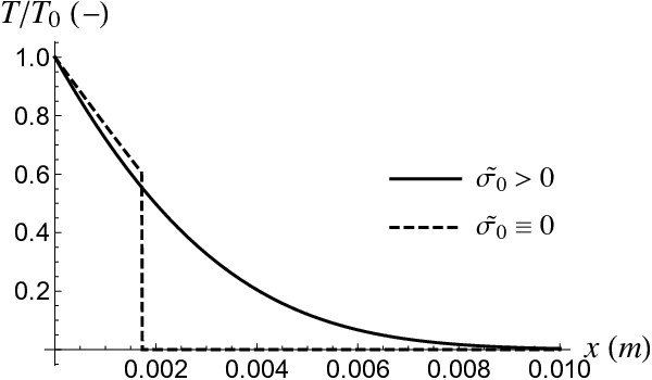
To illustrate this fundamental difference between the thermal transport described by the MC law and the GK-type law used in Farhat et al. 2019, the respective exact solutions of IBVP (5) are shown in Fig. 1 for $\tilde{\sigma}_{0}\equiv 0$ and $\tilde{\sigma}_{0}>0$, respectively. The integral expression for the exact solution obtained by Tanner Tanner 1962 is evaluated numerically using Mathematica’s NIntegrate subroutine, to arbitrary precision, on a finite grid of $x$ values Christov 2010. Figure 1 shows that under the MC law (dashed curve), the heat pulse has only propagated slightly less than 2 mm into the domain. Meanwhile, under the GK law (solid curve), the normalized temperature $T/T_{0}$ is non-zero everywhere in the domain. Since the physical parameter values given in Farhat et al. 2019 are incorrect/inconsistent, to generate the plots in Fig. 1, the values for limestone are taken from Ván et al. 2017, wherein it was experimentally demonstrated that material micro-structure can lead to GK-type heat conduction at room temperature (see also (Berezovski and Ván 2017, Ch. 9)).

To summarize: the behavior of the $\tilde{\sigma}_{0}>0$ case is seen to be strictly diffusive (similar to the solution of the 1D thermal diffusion equation arising from Fourier’s law); the signal applied at $x=0$ is “felt” instantly, but equally, at every point in the half-space $x>0$. In contrast, the $\tilde{\sigma}_{0}\equiv 0$ case predicts a thermal shock-front, of magnitude $T_{0}\exp[-t/(2\tau_{0})]$, propagating (to the right) with finite speed $c_{0}\approx 1.74\times 10^{-3}$ m s^-1 (for the chosen parameter values); see also (Baumeister and Hamill 1969, p. 545) and (Joseph and Preziosi 1989, p. 45).

Returning to Farhat et al.’s analysis, set $\mathcal{S}(\bm{x},t)=0$ and assume $T(\bm{x},t)=\Theta(\bm{x})\exp(-\mathrm{i}\omega t)$, where $\omega(>0)$ is the angular frequency of some thermal disturbance impacting the solid in question. Under these assumptions, Eq. (4) is reduced to the (source-free) Helmholtz equation

It should be noted that, in (Farhat et al. 2019, Eq. (5)), “$T$” is reused instead of introducing a new (time-independent) function such as $\Theta$ herein. (Farhat et al. 2019, Eq. (5)) also incorrectly features the thermal conductivity, with its subscript (“0”) missing, in place of the thermal diffusivity $\varkappa_{0}$.

Consider plane wave propagation in a direction set by the unit vector $\hat{\bm{u}}$. Then, on setting $\Theta(\bm{x})=\Theta_{0}\exp(\mathrm{i}k_{0}\hat{\bm{u}}\cdot\bm{x})$, Eq. (6) yields the dispersion relation

where, $\mathrm{i}=\sqrt{-1}$, $\Theta_{0}>0$ and $k_{0}\in\mathbb{C}$. Enforcing $\Theta<\infty$ as $|\bm{x}|\to\infty$ (and, also, since $\mathfrak{b}>0$) requires $\Imag(k_{0})\geq 0$, then it is readily established that

The dispersion relation in Eq. (8), as well as the $\tilde{\sigma}_{0}\equiv 0$ reduction to its version under the MC law, are illustrated in Fig. 2. Although the dark contours may look similar to (Farhat et al. 2019, Fig. 1(b,bottom)), observe that $\Real(k_{0})<\Imag(k_{0})$ for the chosen set of (realistic) physical parameters, contrary to what is shown in Farhat et al. 2019. However, $\Real(k_{0})>\Imag(k_{0})$ does hold true under the MC law ($\tilde{\sigma}_{0}\equiv 0$). Furthermore, in this case of hyperbolic heat (wave) transfer, the scattering and absorption are not balanced, because $\Imag(k_{0})\to(4\varkappa_{0}\tau_{0})^{-1/2}=const.$ but $\Real(k_{0})\sim\tau_{0}\omega/\sqrt{\varkappa_{0}\tau_{0}}$, as $\tau_{0}\omega\to\infty$.

In addition to those detailed above, the following other errors/issues were noticed in Farhat et al. 2019:

• (i)

  In (Farhat et al. 2019, p. 2), it is claimed that the term proportional to $\sigma_{0}$ is necessary to “make the discretizing process asymptotically stable.” Leaving aside the unclear meaning of “asymptotically” in this context, this statement is false. There is no difficulty whatsoever in discretizing a hyperbolic heat transport equation by any number of methods, as has been known for over three decades (see, e.g., Carey and Tsai 1982; *Glass1985, but note that modern schemes LeVeque 2002 should be used nowadays).

• (ii)

  Below (Farhat et al. 2019, Eq. (5)), it is stated that “$k_{0}$ is a complex number for all frequencies [under the GK-type flux law], which is markedly different from classical heat waves (Fourier transfer).” Setting aside the fact that heat waves are impossible under Fourier’s law, it is clearly seen, on setting $\tau_{0}\equiv 0$ in Eq. (7), that $k_{0}(\omega)=\sqrt{\mathrm{i}\omega/\varkappa_{0}}=(1+\mathrm{i})\sqrt{\omega/(2\varkappa_{0})}\in\mathbb{C}$; i.e., there is no marked difference between Fourier and non-Fourier heat flux laws in this regard.

• (iii)

  The unknown coefficients in the expansions in (Farhat et al. 2019, Eqs. (8) and (9)) are found by applying a boundary condition involving “the temperature field $T$, as well as its flux $\kappa\bm{\nabla}T$.” Under the MC law, the heat flux is not (with misprints corrected) $-\kappa_{0}\bm{\nabla}T$, as it would be under Fourier’s law; rather, it is the expression obtained by solving Eq. (1) for $\bm{\Phi}$. In the case of harmonic time-dependence, for which $\bm{\Phi}(\bm{x},t)=\bm{F}(\bm{x})\exp(-\mathrm{i}\omega t)$, specifying the flux at the boundary of some spatial domain $\mathcal{D}\subset\mathbb{R}^{3}$, under the MC law, would correspond to specifying

  $$\bm{F}=-\left(\frac{1-\mathrm{i}\omega\tau_{0}}{1+\omega^{2}\tau_{0}^{2}}\right)\kappa_{0}\nabla\Theta\quad\text{on}\quad\bm{x}\in\partial\mathcal{D}.$$

  (9)

  The corresponding expression under the GK flux law (2b) is lengthier. This error in imposing the BCs on the series expansion puts into question all subsequent results in (Farhat et al. 2019, Sec. III and IV).

• (iv)

  The conclusion of (Farhat et al. 2019, p. 7) states that “the Fourier heat equation is not frame invariant.” However, this statement is false. The thermal transport equation under Fourier’s law is indeed frame-invariant because the material derivative $DT/Dt:=\partial T/\partial t+\bm{v}\bm{\cdot}\bm{\nabla}T$ is featured on the LHS of Eq. (2a) in its derivation for heat transfer in a moving (or deforming) medium with velocity $\bm{v}$ (see, e.g., (Jog 2015, Sec. 7.1)), whence $DT/Dt\equiv\partial T/\partial t$ if $\bm{v}=\bm{0}$ (stationary conductor). Furthermore, the frame-indifferent formulation of the MC law is misattributed in Farhat et al. 2019; it was, in fact, derived in (Farhat et al. 2019, Ref. 35) not (Farhat et al. 2019, Ref. 43).

• (v)

  The word “photon(s)” should be replaced with “phonon(s)” everywhere in Farhat et al. 2019, given that the context is heat conduction, not electromagnetism.

On the basis of the above-identified errors and stated criticisms, it must be concluded that Farhat et al. Farhat et al. 2019 have failed to provide “the first demonstration of scattering cancellation cloaking for heat waves [emphasis added] obeying the Maxwell–Cattaneo transfer (sic) law.” It would, therefore, be of interest to re-do the study attempted in Farhat et al. 2019, with the correct physical model [i.e., the $\sigma_{0}\equiv 0$ special case of Eqs. (2)], the correct boundary conditions and correct parameter values, to determine whether cloaking is possible (or not).

Finally, with regards to item (iv) above, it is appropriate to mention the promulgation of dubious results. The reworking of classical results under the frame-indifferent generalization of the MC law has generated a large and scientifically/mathematically questionable literature Pantokratoras 2017; *p19; *p19b, which it is easily verified that (Farhat et al. 2019, Ref. 39) is related to.