跳到论文正文
W Papers独立论文阅读器 arXiv:1908.02053 论文正文 计算阅读时间 · 0%
引用这篇论文根据当前论文元数据生成,正式投稿前建议核对。


License: arXiv.org perpetual non-exclusive license
arXiv:1908.02053v2 [cond-mat.stat-mech] 08 Oct 2019

Infinite horizon billiards:
Transport at the border between Gauss and Lévy universality classes

Lior Zarfaty Affiliation: Department of Physics, Institute of Nanotechnology and Advanced Materials, Bar-Ilan University, Ramat-Gan 52900, Israel    Alexander Peletskyi Affiliation: Institute of Physics, University of Augsburg, Universitätsstrasse 1, D-86135 Augsburg, Germany    Eli Barkai Affiliation: Department of Physics, Institute of Nanotechnology and Advanced Materials, Bar-Ilan University, Ramat-Gan 52900, Israel    Sergey Denisov Affiliation: Department of Computer Science, Oslo Metropolitan University, N-0130 Oslo, Norway
Abstract

We consider transport in two billiard models, the infinite horizon Lorentz gas and the stadium channel, presenting analytical results for the spreading packet of particles. We first obtain the cumulative distribution function of traveling times between collisions, which exhibits non-analytical behavior. Using a renewal assumption and the Lévy walk model, we obtain the particles’ probability density. For the Lorentz gas, it shows a distinguished difference when compared with the known Gaussian propagator, as the latter is valid only for extremely long times. In particular, we show plumes of particles spreading along the infinite corridors, creating power-law tails of the density. We demonstrate the slow convergence rate via summation of independent identically distributed random variables on the border between Lévy and Gauss laws. The renewal assumption works well for the Lorentz gas with intermediately sized scattering centers, but fails for the stadium channel due to strong temporal correlations. Our analytical results are supported with numerical samplings.

I Introduction

The infinite horizon Lorentz gas Lorentz is a paradigmatic model of deterministic classical transport, thoroughly studied by physicists Bouchaud; Zaslavsky; Cristadoro1; Cristadoro2; Pedro; Klages; Carlos and mathematicians Bunimovich1; Boldrighini; Bunimovich2; Bleher; Dahlqvist; Szasz; Zaharescu; Chernov1; Chernov2; Chernov3; Marklof1; Dettmann1; Dettmann2; Marklof2. It consists of an infinite periodic lattice of convex obstacles, and point-like particles which undergo elastic collisions with them. The most common configuration of the Lorentz gas model is composed of circular scatterers arranged into an infinite square lattice of unit spacing. Several important properties of this model, such as ergodicity Szasz and algebraic decay of the velocity correlations in time Bunimovich2, have been rigorously proven. Importantly, Bleher Bleher showed that a particle’s position vector 𝒓⁡(t)\boldsymbol{r}(t) has a limiting Gaussian distribution when normalized correctly. More accurately, the quantity limt→∞[𝒓⁡(t)−𝒓⁡(0)]/t​ln⁡(t)\lim_{t\to\infty}[\boldsymbol{r}(t)-\boldsymbol{r}(0)]/\sqrt{t\ln(t)} is a two-dimensional Gaussian variable with zero mean and a covariance matrix which depends on the arrangement of scatterers. However, this asymptotic form is valid only when ln⁡[ln⁡(N)]/ln⁡(N)=ϵ≪1\ln[\ln(N)]/\ln(N)=\epsilon\ll 1, where NN is the number of collisions. To satisfy this condition, NN has to be extremely large (e.g., ϵ=0.01\epsilon=0.01 requires that N≈10281N\approx 10^{281}). Bleher’s time is too large to be physically relevant Zaslavsky, while microscopic inter-collision times cannot describe transport processes happening on much larger time scales. As such, key features of the Lorentz gas model can only be seen for intermediate times that are most relevant for transport regimes. Unfortunately, currently there are no analytical results for these mesoscopic times.

In billiard models, an important characteristic of the transport is a presence (or an absence) of infinite horizons, corridors along which collision-less ballistic trajectories propagate, see Fig. 1. The packet of spreading particles in an infinite horizon billiard models exhibits two main features: the center part of the packet is approximately Gaussian, and the far tails are described by plumes of particles spreading along the infinite corridors. For a specific configuration of the Lorentz gas, we found in our previous Rapid Communication PRE2018 that the scatterers’ geometry is embedded in the cross-like shape of the spreading packet, see Figs. 1 (a) and 2. Here we wish to extend our theory to other configurations, showing its generality. For this aim, we consider the Lorentz gas with corridors forming a British flag-like structure for the packet of spreading particles, seen in Figs. 1 (b) and 3, together with a quasi one-dimensional transport in a chain of concatenated Bunimovich billiard stadiums Bunimovich1; Zaslavsky, seen in Figs. 1 (c) and 4. While the models are distinctive, along the corridors the far tails of the density decay spatially with a universal power-law, a feature well described by the Lévy walk model Levy1; Levy2; Levy3; Levy4.

Our analysis is composed of two main ingredients, one of them is obtaining the aforementioned billiard systems’ full distribution of inter-collision times. For the Lorentz gas, results in the limits of R→1R\to 1 and τ→∞\tau\to\infty (where RR is a scatterer’s radius and τ\tau is an inter-collision time) were found by Bouchaud and Le Doussal Bouchaud. More recently, an asymptotic form in the limit of R→0R\to 0 was established Dahlqvist; Zaharescu; Marklof1. However, this important aspect in the characterization of transport is hardly discussed in the literature when finite sized scatterers are considered. This distribution’s probability density function (PDF) exhibits a far tail obeying

limτ→∞τ3​ψ​(τ)=τ02,\lim_{\tau\to\infty}\tau^{3}\psi(\tau)=\tau_{0}^{2}, (1)

which is valid for both limits of large and small scatterers. Therefore, we use a Lévy walk model with exponent −3-3 for the other ingredient, which is calculating the density of spreading particles. A principal issue here is that in a Lévy walk approximation one uses a renewal assumption, i.e. one neglects correlations between consecutive collisions. It was shown that for the cross-like configuration of the Lorentz gas and in the limit of large scattering centers, this condition is nullified as an effective trapping mechanism emerges Cristadoro1. In contrast, when the scattering centers are not too large, the Lévy walk with the obtained cumulative distribution function (CDF) of the waiting times works perfectly, as demonstrated below. Deviations from the renewal theory do exist for the stadium channel model where correlations are strong, as we show below. However, this does not imply that the Lévy walk model is not predictive here as well, and in fact we find the opposite. Another primary issue is caused since these two systems are operating on the border between Gauss and Lévy central limit theorems, due to the exponent −3-3 which causes a logarithmic divergence of ψ⁡(τ)\psi(\tau)’s second moment. Thus, an ultra-slow convergence rate problem arises that can be understood via a toy model: summation of independent identically distributed (IID) random variables (RVs), with a common symmetric PDF that decays algebraically with a power of −3-3 for large argument. Already here we encounter the same type of convergence problem discussed in the first paragraph, which is neutralized using what we call Lambert scaling approach. This is a crucial step for these systems, as it allows us to compare finite time simulations with our theory for duration regimes where previous results do not hold.

The rest of this paper is organized as follows: in section II we provide an example of the Lambert scaling for sums of IID RVs. In section III we derive the main formula of the spatial PDFs by using the Lévy walk model. In section IV we obtain the CDFs of inter-collision times for the Lorentz gas and stadium channel. We discuss our results in section V.

Figure 1: The considered models, the infinite horizon Lorentz gas with two (a) and four (b) open horizons, and the stadium channel model (c). For the Lorentz gas we take the lattice constant to be 11, while for the stadium channel we use 11 for the radius of a semicircle wall. The parameter which controls the qualitative behavior for the Lorentz gas is the scatterers’ radius RR. When 1/8≤R<1/21/\sqrt{8}\leq R<1/2, there are two directions of infinite corridors. A particle that collided with the black circle can fly along the blue solid arrows, reaching scatterers along them. Decreasing the radius such that 1/20≤R<1/81/\sqrt{20}\leq R<1/\sqrt{8} creates additional two directions of infinite corridors. A particle that collided with the black circle can now fly along the red dashed arrows as well (see Fig. 7 for additional details). In the stadium channel model the controlling parameter is the walls’ separation, D>0D>0. A particle which was scattered from the thick bottom semicircle can reach any stadium of the top row, but can also hit the origin semicircle again (the dashed stadiums are unreachable in this case). All of the numerical simulations were performed using unit speed, namely V=1V=1.

II A simplified case of Lambert scaling

We now consider the problem of summation of IID RVs, drawn from a power-law distribution. We work at the border between Gauss and Lévy central limit theorems, which is clearly related to the exponent −3-3 in Eq. (1). Some aspects of this by far simpler approach are important for the discussed billiard models. In particular, at this transition we find a critical slowing down in the sense that convergence to the Gaussian limit theorem is ultra-slow Greengard, a problem which is resolved by Lambert scaling. Consider a sum of N≫1N\gg 1 IID RVs

x=∑n=1Nχn,x=\sum_{n=1}^{N}\chi_{n}, (2)

where the summands are drawn from a common symmetric PDF which obeys f⁡(χ→∞)≃χ02/χ3f(\chi\to\infty)\simeq\chi_{0}^{2}/\chi^{3}. We define the scaled sum as x¯=x/χ02​N​Ω​(N)/2\bar{x}=x/\sqrt{\chi_{0}^{2}N\Omega(N)/2} with N​Ω​(N)N\Omega(N) being a scaling parameter, soon to be determined. We use the characteristic function

⟨exp⁡(i​k¯​x¯)⟩=exp⁡{N​ln⁡[f~​(k¯χ02​N​Ω​(N)/2)]},\langle\exp(i\bar{k}\bar{x})\rangle=\exp\left\{N\ln\left[\tilde{f}\left(\frac{\bar{k}}{\sqrt{\chi_{0}^{2}N\Omega(N)/2}}\right)\right]\right\}, (3)

where f~​(k)\tilde{f}(k) is the Fourier transform of f⁡(χ)f(\chi). Assuming that Ω⁡(N)\Omega(N) monotonically increases with NN, the small kk behavior of f~​(k)\tilde{f}(k) is considered

f~​(k)≃1+12​(χ0​k)2​ln⁡[(Cf​χ0​k)2],\tilde{f}(k)\simeq 1+\frac{1}{2}\left(\chi_{0}k\right)^{2}\ln\left[\left(C_{f}\chi_{0}k\right)^{2}\right], (4)

which is derived in appendix A. The first term is the normalization, while the second is related to the power-law tail of f⁡(χ)f(\chi), with CfC_{f} being

Cf=exp{γ\displaystyle C_{f}=\exp\left\{\vphantom{\int_{\chi_{0}}^{\infty}\text{d}\chi\left[f(\chi)\left(\frac{\chi}{\chi_{0}}\right)^{2}-\frac{1}{\chi}\right]}\gamma\right. −32−∫0χ0d​χ​f​(χ)​(χχ0)2\displaystyle-\frac{3}{2}-\int_{0}^{\chi_{0}}\text{d}\chi\,f(\chi)\left(\frac{\chi}{\chi_{0}}\right)^{2} (5)
−∫χ0∞dχ[f(χ)(χχ0)2−1χ]},\displaystyle-\left.\int_{\chi_{0}}^{\infty}\text{d}\chi\left[f(\chi)\left(\frac{\chi}{\chi_{0}}\right)^{2}-\frac{1}{\chi}\right]\right\},

where γ≈0.5772\gamma\approx 0.5772 is Euler’s constant. Inserting Eq. (4) into Eq. (3) and expanding, we get

⟨exp⁡(i​k¯​x¯)⟩≃exp⁡{k¯2Ω⁡(N)​ln⁡[2​Cf2​k¯2N​Ω​(N)]}.\left<\exp(i\bar{k}\bar{x})\right>\simeq\exp\left\{\frac{\bar{k}^{2}}{\Omega(N)}\ln\left[\frac{2C_{f}^{2}\bar{k}^{2}}{N\Omega(N)}\right]\right\}. (6)

We now determine the slowly increasing function Ω⁡(N)\Omega(N) with the choice

ln⁡[N​Ω​(N)2​Cf2]=Ω⁡(N),\ln\left[\frac{N\Omega(N)}{2C_{f}^{2}}\right]=\Omega(N), (7)

which yields

Ω⁡(N)=|W−1​(−2​Cf2N)|.\Omega(N)=\left|\text{W}_{-1}\left(-\frac{2C_{f}^{2}}{N}\right)\right|. (8)

Here W−1​(η)\text{W}_{-1}(\eta) is the secondary branch of the Lambert W-function Functions, defined for η∈[−1/e,0)\eta\in[-1/e,0) by the identity W−1​(η)=ln⁡[η/W−1​(η)]\text{W}_{-1}(\eta)=\ln[\eta/\text{W}_{-1}(\eta)]. The Lambert function has the following expansion as η→0−\eta\rightarrow 0^{-}

|W−1​(η)|=L1+L2+L2L1+𝒪⁡(L22L12),\left|\text{W}_{-1}(\eta)\right|=L_{1}+L_{2}+\frac{L_{2}}{L_{1}}+\mathcal{O}\left(\frac{L_{2}^{2}}{L_{1}^{2}}\right), (9)

where L1=ln⁡(1/|η|)L_{1}=\ln(1/|\eta|) and L2=ln⁡[ln⁡(1/|η|)]L_{2}=\ln[\ln(1/|\eta|)]. Equations (8) and (9) yield N​Ω​(N)≃N​ln⁡(N)N\Omega(N)\simeq N\ln(N) when N→∞N\to\infty, reproducing the well-known Gnedenko-Kolmogorov scaling N​ln⁡(N)\sqrt{N\ln(N)} Limit. However, for this to be of relevance, one must demand ln⁡(N)≫ln⁡[ln⁡(N)]\ln(N)\gg\ln[\ln(N)], which makes the convergence to this mathematical limit ultra-slow. Our Lambert scaling approach unites all of the NN-dependent logarithmic terms into a single function, thus resolving this problem. We therefore expand Eq. (6) for large Ω⁡(N)\Omega(N), keeping terms up to sub-leading order during the calculation

⟨exp⁡(i​k¯​x¯)⟩≃e−k¯2​[1+k¯2Ω⁡(N)​ln⁡(k¯2)].\left<\exp(i\bar{k}\bar{x})\right>\simeq e^{-\bar{k}^{2}}\left[1+\frac{\bar{k}^{2}}{\Omega(N)}\ln\left(\bar{k}^{2}\right)\right]. (10)

Inverting Eq. (10) back to position space, we reach our first result, the PDF of xx

P(x,N)≃1π​ξ2​(N)exp[−x2ξ2​(N)]×\displaystyle P(x,N)\simeq\frac{1}{\sqrt{\pi\xi^{2}(N)}}\exp\left[-\frac{x^{2}}{\xi^{2}(N)}\right]\times
{1+1Ω⁡(N){[2−γ−ln(4)][12−x2ξ2​(N)]\displaystyle\left\{1+\frac{1}{\Omega(N)}\left\{\left[2-\gamma-\ln(4)\vphantom{\frac{1}{2}}\right]\left[\frac{1}{2}-\frac{x^{2}}{\xi^{2}(N)}\right]\right.\right.
−12M(1,0,0)[−1;12;x2ξ2​(N)]}},\displaystyle\left.\left.-\frac{1}{2}\text{M}^{(1,0,0)}\left[-1;\frac{1}{2};\frac{x^{2}}{\xi^{2}(N)}\right]\right\}\right\}, (11)

with ξ⁡(N)=2​χ02​N​Ω​(N)\xi(N)=\sqrt{2\chi_{0}^{2}N\Omega(N)}. Here M​(⋯)\text{M}(\cdots) is Kummer’s confluent hypergeometric function Functions, and the superscript over M denotes its derivative with respect to its first argument. Figure 5 shows a good match between Eq. (II) and the sum Eq. (2)’s PDF for two different common density functions, f⁡(χ)f(\chi) and g⁡(χ)g(\chi) which are defined in the caption, with N=104N=10^{4}. The Kummer function behave asymptotically as M(1,0,0)(−1,1/2,η2)≃−πexp(η2)/η3\text{M}^{(1,0,0)}(-1,1/2,\eta^{2})\simeq-\sqrt{\pi}\exp(\eta^{2})/\eta^{3}, suggesting that P⁡(x,N)≃N​χ02/x3P(x,N)\simeq N\chi_{0}^{2}/x^{3}. Thus, the PDF of the sum xx reproduces the same power-law tails as of the original common PDF f⁡(χ)f(\chi). As the distribution of traveling times between collisions Eq. (1) exhibit the same heavy-tail exponent of −3-3, our next step is implementing Lambert scaling to the Lévy walk model.

Refer to caption
Figure 2: The position’s probability density function for the Lorentz gas with two open horizons produces a cross-like geometry. Here, the lattice constant and speed are 11, the scatterers’ radius is R=0.4R=0.4, and the time duration is t=104t=10^{4}. The Lorentz gas simulation (a) has approximately 10910^{9} sampled trajectories. Our theory Eq. (III) with q=0q=0 reproduces the simulation well (b).
Refer to caption
Figure 3: The position’s probability density function for the Lorentz gas with four open horizons produces a British flag-like shape. Here, the lattice constant and speed are 11, the scatterers’ radius is R=0.3R=0.3, and the time duration is t=104t=10^{4}. The Lorentz gas simulation (a) is reproduced without any fitting by our theory (b), which is given by Eqs. (III) and (47).
Refer to caption
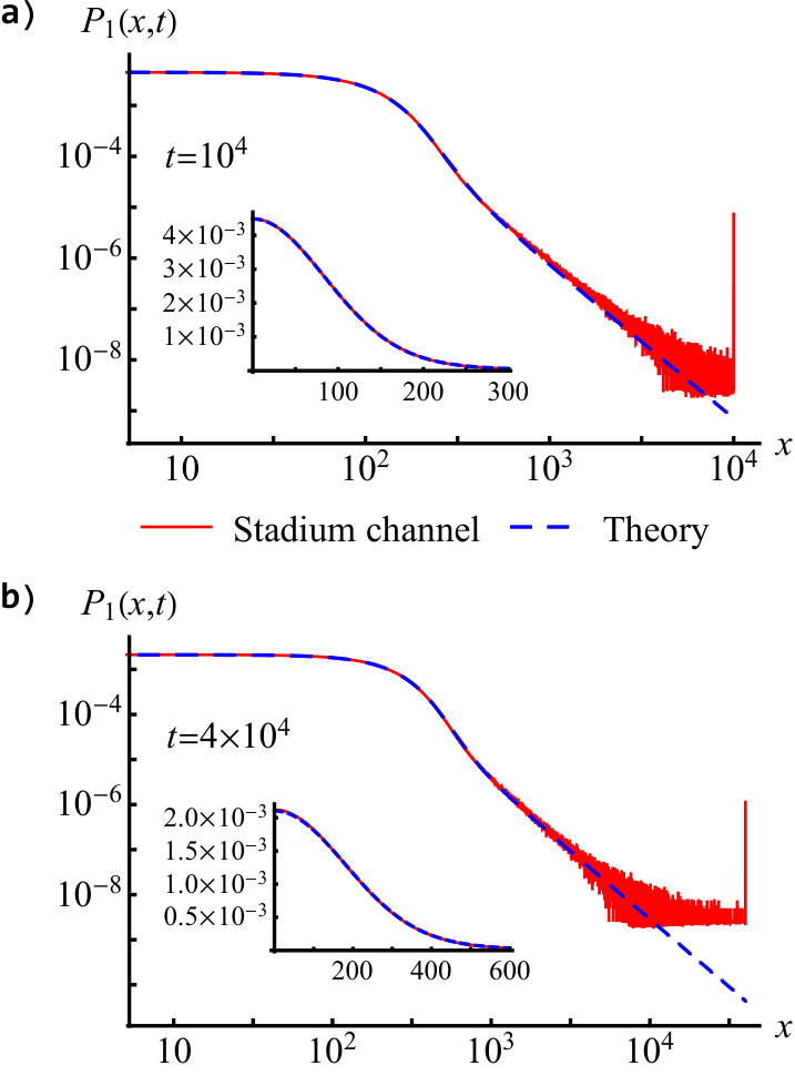
Figure 4: The position’s probability density function of the stadium channel model for t=104t=10^{4} (a) and t=4×10⁴t=4\times 10^{4} (b), with D=1D=1. Solid red is the stadium channel numerical simulations, dashed blue is Eq. (III). Using a two parameter fitting procedure and the simulation of duration t=104t=10^{4}, we find that Cψ2​⟨τ⟩≈0.3776C_{\psi}^{2}\langle\tau\rangle\approx 0.3776 and ⟨τ⟩/τ02≈7.0607\langle\tau\rangle/\tau_{0}^{2}\approx 7.0607. These values were used when calculating P1​(x,t)P_{1}(x,t) for t=4×10⁴t=4\times 10^{4}. The curves match well, which means that Eq. (III) can indeed describe the stadium channel model, given an “effective" waiting times distribution. The stadium channel simulations have around 2×1082\times 10^{8} sampled trajectories (the smallest values in the histograms represent cells with a single event).
Figure 5: The probability density function (PDF) of the sum Eq. (2) with N=104N=10^{4}, and its corresponding Lambert scaling approximation Eq. (II). The common PDFs used here are f⁡(χ)=1/|χ|3f(\chi)=1/|\chi|^{3} when |χ|≥1|\chi|\geq 1, and 00 otherwise (a), and g(χ)=(1+χ2)−3/2/2g(\chi)=(1+\chi^{2})^{-3/2}/2 (b). The exact values (solid) are obtained from an inverse Fourier transform of f~N​(k)\tilde{f}^{N}(k), dashed lines are the theory Eq. (II), and dot-dashed are the limit distributions of Gnedenko-Kolmogorov (G-K) Limit.

III Lambert scaling of the Lévy walk model

The dd-dimensional Lévy walk model Levy2; Levy4 is defined as follows: a random walker is placed at 𝒓⁡(0)\boldsymbol{r}(0) on time t=0t=0. Its movement consists of segments of ballistic motion with constant velocity, separated by collision-like events which induce a change in the velocity’s magnitude and/or direction. The process lasts for a fixed duration, which is the measurement time tt. The model employs two PDFs in order to determine the displacement during each of the ballistic motion epochs. The velocity of each segment is drawn from a PDF Fd​(𝒗)F_{d}(\boldsymbol{v}), whose moments are all finite, and is further assumed to be symmetric with respect to each of the components vjv_{j} where 1≤j≤d1\leq j\leq d (such that its odd moments vanish). The time duration of each ballistic section is drawn from a PDF ψ⁡(τ)\psi(\tau). The movement continues until the allotted measurement time is met, thus the number of collisions NN in [0,t][0,t] is random. This yields the total displacement as

𝒓⁡(t)−𝒓⁡(0)=∑n=1N𝒗n−1​τn+𝒗N​τb,\boldsymbol{r}(t)-\boldsymbol{r}(0)=\sum_{n=1}^{N}\boldsymbol{v}_{n-1}\tau_{n}+\boldsymbol{v}_{N}\tau_{b}, (12)

where τn\tau_{n} is the traveling time of the nnth walking epoch, 𝒗n\boldsymbol{v}_{n} is the velocity after the nnth collision, and the initial conditions 𝒓⁡(0)\boldsymbol{r}(0) and 𝒗0\boldsymbol{v}_{0} are randomly chosen. The traveling times and velocities {τn,𝒗n}\{\tau_{n},\boldsymbol{v}_{n}\} (with 1≤n≤N1\leq n\leq N) are IID RVs, with the last movement duration being τb=t−∑n=1Nτn\tau_{b}=t-\sum_{n=1}^{N}\tau_{n}. Notice that the measurement time divided by the mean time between collisions, t/⟨τ⟩t/\langle\tau\rangle, and the lengths of inter-collision travel, {𝒗n−1​τn}\{\boldsymbol{v}_{n-1}\tau_{n}\}, roughly correspond to NN and {χn}\{\chi_{n}\} from the previous section, respectively. We denote the particle’s speed with VV, which is kept unchanged in the billiards systems due to the collisions’ elasticity (in the numerical simulations V=1V=1). Let us denote the probability to find the walker at position 𝒓\boldsymbol{r} on time tt as Pd​(𝒓,t)P_{d}(\boldsymbol{r},t), and let Πd​(𝒌,u)\Pi_{d}(\boldsymbol{k},u) be its Fourier and Laplace transform

Πd​(𝒌,u)=∫dd​r​∫0∞d​t​Pd​(𝒓,t)​e−u​t+i​𝒌⋅𝒙.\Pi_{d}\left(\boldsymbol{k},u\right)=\int\text{d}^{d}r\int_{0}^{\infty}\text{d}tP_{d}\left(\boldsymbol{r},t\right)e^{-ut+i\boldsymbol{k}\cdot\boldsymbol{x}}. (13)

An exact expression of Πd​(𝒌,u)\Pi_{d}(\boldsymbol{k},u) is given by the Montroll-Weiss equation MW

Πd​(𝒌,u)=⟨1−ψ^​(u−i​𝒌⋅𝒗)u−i​𝒌⋅𝒗⟩​11−⟨ψ^​(u−i​𝒌⋅𝒗)⟩,\Pi_{d}\left(\boldsymbol{k},u\right)=\left<\frac{1-\hat{\psi}\left(u-i\boldsymbol{k}\cdot\boldsymbol{v}\right)}{u-i\boldsymbol{k}\cdot\boldsymbol{v}}\right>\frac{1}{1-\left<\hat{\psi}\left(u-i\boldsymbol{k}\cdot\boldsymbol{v}\right)\right>}, (14)

where ψ^​(u)\hat{\psi}(u) is the Laplace transform of ψ⁡(τ)\psi(\tau), defined as

ψ^​(u)=∫0∞d​τ​ψ​(τ)​e−u​τ,\hat{\psi}(u)=\int_{0}^{\infty}\text{d}\tau\,\psi(\tau)e^{-u\tau}, (15)

and

⟨⋯⟩=∫ddv⋯Fd(𝒗),\left<\cdots\right>=\int\text{d}^{d}v\cdots F_{d}(\boldsymbol{v}), (16)

with the above integral carried over all velocity space.

We now direct the reader’s attention to two points before advancing with the calculation. First, notice that the assumption of finite moments for the velocity distribution Fd​(𝒗)F_{d}(\boldsymbol{v}) is crucial to our theory. For example, a diverging second moment yields Lévy statistics in the bulk instead of a Gaussian, whereas for the Lorentz gas it is rigorously proven to be the latter case Bleher. Second, in Ref. Levy4 the authors discuss two different variations of Lévy walk: the velocity model and the jump model. For the former, particles move constantly until the measurement time ends, their last traveling epoch being τb\tau_{b}. However, for the latter particles are missing this final segment of walk. Therefore, the two models differ only when considering approximation theories of the far tail (under the condition of finite mean time between collisions). As our theory is intended to approximate the bulk of the PDF P⁡(𝒓,t)P(\boldsymbol{r},t), these two aforementioned cases are indistinguishable. Technically speaking, this difference is manifested by a different numerator of Eq. (14), which does not change its approximated versions which appear below, Eqs. (20) and (III). Further, in the Lorentz gas a particle’s velocity is unity at any moment of travel, therefore the velocity model is more suitable if compared to the jump model.

To approximate Eq. (14) we use the asymptotic behavior of ψ⁡(τ)\psi(\tau) Eq. (1), which implies that for small uu

ψ^​(u)≃1−⟨τ⟩​u−12​(τ0​u)2​ln⁡(Cψ​τ0​u),\hat{\psi}(u)\simeq 1-\langle\tau\rangle u-\frac{1}{2}\left(\tau_{0}u\right)^{2}\ln\left(C_{\psi}\tau_{0}u\right), (17)

which is derived in appendix B. Here, the first term is the normalization, ⟨τ⟩\langle\tau\rangle is the mean time between collisions, and the last term is related to the power-law tail of ψ⁡(τ)\psi(\tau), with CψC_{\psi} being

Cψ=exp{γ\displaystyle C_{\psi}=\exp\left\{\vphantom{\int_{\tau_{0}}^{\infty}\text{d}\tau\left[\psi(\tau)\left(\frac{\tau}{\tau_{0}}\right)^{2}-\frac{1}{\tau}\right]}\gamma\right. −32−∫0τ0d​τ​ψ​(τ)​(ττ0)2\displaystyle-\frac{3}{2}-\int_{0}^{\tau_{0}}\text{d}\tau\,\psi(\tau)\left(\frac{\tau}{\tau_{0}}\right)^{2} (18)
−∫τ0∞dτ[ψ(τ)(ττ0)2−1τ]}.\displaystyle-\left.\int_{\tau_{0}}^{\infty}\text{d}\tau\left[\psi(\tau)\left(\frac{\tau}{\tau_{0}}\right)^{2}-\frac{1}{\tau}\right]\right\}.

We assume a scaling of u∼k2​L​(k)u\sim k^{2}L(k), where L⁡(⋯)L(\cdots) is some logarithmic-like function and k=|𝒌|k=|\boldsymbol{k}|. This suggests that u≪ku\ll k when k→0k\rightarrow 0, and as such we can expand the Montroll-Weiss Eq. (14) in the small parameter u/k​vu/kv where v=|𝒗|v=|\boldsymbol{v}|, see appendix C. For the one-dimensional stadium channel model, we apply the following distribution of velocities

F1​(vx)=12​[δ⁡(vx−V)+δ⁡(vx+V)],F_{1}\left(v_{x}\right)=\frac{1}{2}\left[\delta\left(v_{x}-V\right)+\delta\left(v_{x}+V\right)\vphantom{\frac{1}{2}}\right], (19)

where in our case V=1V=1. We obtain in appendix C the following Fourier expansion for the distribution

P~1​(κx,t)≃2​e−κx2ξ1​(t)​[1+1Ω1​(t)​κx2​ln⁡(κx2)],\tilde{P}_{1}(\kappa_{x},t)\simeq\frac{2e^{-\kappa_{x}^{2}}}{\xi_{1}(t)}\left[1+\frac{1}{\Omega_{1}(t)}\kappa_{x}^{2}\ln\left(\kappa_{x}^{2}\right)\right], (20)

with

Ωd​(t)=|W−1​(−4​d​Cψ2​⟨τ⟩t)|,\displaystyle\Omega_{d}(t)=\left|\text{W}_{-1}\left(-4dC_{\psi}^{2}\frac{\left<\tau\right>}{t}\right)\right|,
ξd​(t)=τ02​⟨v2⟩​t​Ωd​(t)d​⟨τ⟩,\displaystyle\xi_{d}(t)=\sqrt{\tau_{0}^{2}\langle v^{2}\rangle\frac{t\Omega_{d}(t)}{d\langle\tau\rangle}}, (21)

where here and for the following Lorentz gas ⟨v2⟩=V2\langle v^{2}\rangle=V^{2}. The walker’s position PDF in dd spatial dimensions is given by the inverse Fourier transform

Pd​(𝒓,t)=∫dd​κ(2​π)d​P~d​(𝜿,t)​cos⁡[2​(𝜿⋅𝒓)ξd​(t)].P_{d}(\boldsymbol{r},t)=\int\frac{\text{d}^{d}\kappa}{(2\pi)^{d}}\tilde{P}_{d}\left(\boldsymbol{\kappa},t\right)\cos\left[\frac{2(\boldsymbol{\kappa}\cdot\boldsymbol{r})}{\xi_{d}(t)}\right]. (22)

Inserting Eq. (20) into Eq. (22) results with

P1​(x,t)\displaystyle P_{1}(x,t) =1π​ξ12​(t)​exp⁡[−x2ξ12​(t)]\displaystyle=\frac{1}{\sqrt{\pi\xi_{1}^{2}(t)}}\exp\left[-\frac{x^{2}}{\xi_{1}^{2}(t)}\right]
×{1+1Ω1​(t){[2−γ−ln(4)][12−x2ξ12​(t)]\displaystyle\times\left\{1+\frac{1}{\Omega_{1}(t)}\left\{\left[2-\gamma-\ln(4)\vphantom{\frac{x^{2}}{\xi_{1}^{2}(t)}}\right]\left[\frac{1}{2}-\frac{x^{2}}{\xi_{1}^{2}(t)}\right]\right.\right.
−12M(1,0,0)[−1;12;x2ξ12​(t)]}}.\displaystyle-\left.\left.\frac{1}{2}\text{M}^{(1,0,0)}\left[-1;\frac{1}{2};\frac{x^{2}}{\xi_{1}^{2}(t)}\right]\right\}\right\}. (23)

The subscript 11 stands for one dimension, namely this result should hold for the stadium channel when we coarse grain over the channel’s width. We see some similarities with the problem of summation of IID RVs. For example, Kummer’s function appears in both problems as a correction to the leading term. There is however a major difference between the two cases: here P⁡(𝒓,t)=0P(\boldsymbol{r},t)=0 for 𝒓>t\boldsymbol{r}>t, which is different from the problem of summation of IID RVs. This is clearly due to the particles’ finite speed. For the two-dimensional Lorentz gas model with two/four infinite horizons we have

F2​(𝒗)\displaystyle F_{2}\left(\boldsymbol{v}\right) =1−q4{[δ(vx−V)+δ(vx+V)]δ(vy)\displaystyle=\frac{1-q}{4}\left\{\left[\delta\left(v_{x}-V\right)+\delta\left(v_{x}+V\right)\vphantom{\frac{v_{\times}}{\sqrt{2}}}\right]\delta\left(v_{y}\right)\right.
+δ(vx)[δ(vy−V)+δ(vy+V)]}\displaystyle+\left.\delta\left(v_{x}\right)\left[\delta\left(v_{y}-V\right)+\delta\left(v_{y}+V\right)\vphantom{\frac{v_{\times}}{\sqrt{2}}}\right]\right\}
+q4{[δ(vx−V2)+δ(vx+V2)]\displaystyle+\frac{q}{4}\left\{\left[\delta\left(v_{x}-\frac{V}{\sqrt{2}}\right)+\delta\left(v_{x}+\frac{V}{\sqrt{2}}\right)\right]\right.
×[δ(vy−V2)+δ(vy+V2)]},\displaystyle\times\left.\left[\delta\left(v_{y}-\frac{V}{\sqrt{2}}\right)+\delta\left(v_{y}+\frac{V}{\sqrt{2}}\right)\right]\right\}, (24)

where q≥0q\geq 0 is a parameter to be determined later, which encodes the probability of a particle to be found in the far tail of the diagonal corridors (for two open horizons, a cross-shape, one has q=0q=0). We get from Eq. (14)

P~2​(𝜿,t)\displaystyle\tilde{P}_{2}(\boldsymbol{\kappa},t) ≃4​e−κx2−κy2ξ22​(t)\displaystyle\simeq\frac{4e^{-\kappa_{x}^{2}-\kappa_{y}^{2}}}{\xi_{2}^{2}(t)}
×{1+1−qΩ2​(t)[κx2ln(κx2)+κy2ln(κy2)]\displaystyle\times\left\{1+\frac{1-q}{\Omega_{2}(t)}\left[\kappa_{x}^{2}\ln\left(\kappa_{x}^{2}\right)+\kappa_{y}^{2}\ln\left(\kappa_{y}^{2}\right)\vphantom{\frac{1}{2}}\right]\right.
+q2​Ω2​(t)​(κx+κy)2​ln⁡[12​(κx+κy)2]\displaystyle+\frac{q}{2\Omega_{2}(t)}\left(\kappa_{x}+\kappa_{y}\right)^{2}\ln\left[\frac{1}{2}\left(\kappa_{x}+\kappa_{y}\right)^{2}\right]
+q2​Ω2​(t)(κx−κy)2ln[12(κx−κy)2]}.\displaystyle+\left.\frac{q}{2\Omega_{2}(t)}\left(\kappa_{x}-\kappa_{y}\right)^{2}\ln\left[\frac{1}{2}\left(\kappa_{x}-\kappa_{y}\right)^{2}\right]\right\}. (25)

We use a π/4\pi/4 rotation transformation κ±=(κx±κy)/2\kappa_{\pm}=(\kappa_{x}\pm\kappa_{y})/\sqrt{2} to calculate the integrals over Eq. (III)’s last two terms, and obtain

P2​(𝒓,t)\displaystyle P_{2}(\boldsymbol{r},t) ≃1π​ξ22​(t)​exp⁡[−x2+y2ξ22​(t)]\displaystyle\simeq\frac{1}{\pi\xi_{2}^{2}(t)}\exp\left[-\frac{x^{2}+y^{2}}{\xi_{2}^{2}(t)}\right]
×{1+1Ω2​(t){[2−γ−ln(4)][1−x2+y2ξ22​(t)]\displaystyle\times\left\{1+\frac{1}{\Omega_{2}(t)}\left\{\left[2-\gamma-\ln(4)\vphantom{\frac{x^{2}}{\xi_{2}^{2}(t)}}\right]\left[1-\frac{x^{2}+y^{2}}{\xi_{2}^{2}(t)}\right]\right.\right.
−1−q2​M(1,0,0)​[−1;12;x2ξ22​(t)]\displaystyle-\frac{1-q}{2}\text{M}^{(1,0,0)}\left[-1;\frac{1}{2};\frac{x^{2}}{\xi_{2}^{2}(t)}\right]
−1−q2​M(1,0,0)​[−1;12;y2ξ22​(t)]\displaystyle-\frac{1-q}{2}\text{M}^{(1,0,0)}\left[-1;\frac{1}{2};\frac{y^{2}}{\xi_{2}^{2}(t)}\right]
−q2​M(1,0,0)​[−1;12;(x+y)22​ξ22​(t)]\displaystyle-\frac{q}{2}\text{M}^{(1,0,0)}\left[-1;\frac{1}{2};\frac{(x+y)^{2}}{2\xi_{2}^{2}(t)}\right]
−q2M(1,0,0)[−1;12;(x−y)22​ξ22​(t)]}},\displaystyle\left.\left.-\frac{q}{2}\text{M}^{(1,0,0)}\left[-1;\frac{1}{2};\frac{(x-y)^{2}}{2\xi_{2}^{2}(t)}\right]\right\}\right\}, (26)

where the subscript 22 stands for two dimensions. This solution is presented in Figs. 2 and 3, with the relevant parameters, namely τ0\tau_{0}, ⟨τ⟩\langle\tau\rangle, CψC_{\psi} and qq, obtained from ψ⁡(τ)\psi(\tau) [more precisely we extract them out of CDF​(τ)\text{CDF}(\tau)]. Thus, we continue with deriving exact expressions for the distribution of traveling times ψ⁡(τ)\psi(\tau) for the Lorentz gas model with two/four open infinite corridors and for the stadium channel model. To refrain from cumbersome formulas, we omit some of the next section’s derivations. Please refer to appendix D for more details.

Figure 6: The parameters which determine the trajectory’s length for the Lorentz gas model (a) and stadium channel model (b). For the Lorentz gas, the lattice coordinates of the next scatterer to be collided with are denoted as (n,m)(n,m), the recoil angle after the previous collision is β\beta, and the impact parameter is bb. In this sketch, we used n=1n=1, m=0m=0, β=π/6\beta=\pi/6, b=−0.3b=-0.3 and R=0.4R=0.4, which correspond to τn,m∗​(b,β,R)≈0.255\tau_{n,m}^{*}(b,\beta,R)\approx 0.255 (the lattice constant is 11). For the stadium channel, we denote as (2​n,m)(2n,m) the lattice site of the next stadium to be collided with, where α\alpha is the recoil angle after the previous collision and aa is an “impact parameter". Here we used n=1n=1, m=Dm=D, α=π/6\alpha=\pi/6, a=−0.4a=-0.4 and D=1D=1, which correspond to τ2​n,m∗​(a,α)≈4.11\tau_{2n,m}^{*}(a,\alpha)\approx 4.11 (the semicircles’ radius is 11).
Figure 7: In the Lorentz gas, a tracer particle right after a collision with the origin circle (solid black) can hit only the colored scatteres. These are made of three distinct groups: four nearest neighbors (vertical blue), four next to nearest neighbors (horizontal green), and eight clusters of distant neighbors (chess red). The white circles are inaccessible for the particle. Given a lattice constant 11, for a scatterers’ radius of R=0.4R=0.4 (a) one has two directions for possible infinite trajectories, directed with the lattice axes. For a scatterers’ radius of R=0.3R=0.3 (b) two diagonal infinite directions are added, and the particle can now reach the yellow scatterers (solid light gray in print). When calculating the cumulative distribution function of the traveling times between collisions, we sum the contribution of each scatterer to the trajectories’ space, see section IV. Exploiting the noticeable symmetry, we focus on the black rectangle-encircled area (a), and additionally the black ellipse-encircled area when RR is decreased (b).

IV The distribution of traveling times

IV.1 Lorentz gas model

To obtain the distribution of traveling times we define a 2​d2d cubic lattice of constant 11 occupied with circular scatterers of radius RR, such that the center of each circle is located at a grid point, see Fig. 1 (a) and (b). Let the lattice coordinates of each scatterer be (n,m)(n,m), where nn and mm are integers. We focus on the origin, and assume that the particle has just collided with the (0,0)(0,0) scatterer. We define the collision’s impact parameter and recoil direction as bb and β\beta respectively, see Fig. 6 (a), where the ranges of values for these two parameters are [−R,R][-R,R] and [0,2​π)[0,2\pi), respectively. We denote as τn,m∗​(b,β,R)\tau_{n,m}^{*}(b,\beta,R) the time duration until the following collision, and since V=1V=1 it is also the distance traveled. Here, we assume that the next scatterer to be collided with is the (n,m)(n,m) one. The expression obtained for τn,m∗​(b,β,R)\tau_{n,m}^{*}(b,\beta,R) is

τn,m∗​(b,β,R)\displaystyle\tau_{n,m}^{*}(b,\beta,R) =n​cos⁡(β)+m​sin⁡(β)−R2−b2\displaystyle=n\cos(\beta)+m\sin(\beta)-\sqrt{R^{2}-b^{2}}
−R2−[m​cos⁡(β)−n​sin⁡(β)−b]2.\displaystyle-\sqrt{R^{2}-\left[m\cos(\beta)-n\sin(\beta)-b\right]^{2}}. (27)

We then write the PDF ψ⁡(τ)\psi(\tau) as

ψ⁡(τ)=\displaystyle\psi(\tau)= (28)
∑n,m∫βn,mmin​(R)βn,mmax​(R)d​β2​π​∫bn,mmin​(β,R)bn,mmax​(β,R)d​b2​R​δ​[τ−τn,m∗​(b,β,R)],\displaystyle\sum_{n,m}\int_{\beta_{n,m}^{\rm min}(R)}^{\beta_{n,m}^{\rm max}(R)}\frac{\text{d}\beta}{2\pi}\int_{b_{n,m}^{\rm min}(\beta,R)}^{b_{n,m}^{\rm max}(\beta,R)}\frac{\text{d}b}{2R}\;\delta\left[\tau-\tau^{*}_{n,m}(b,\beta,R)\vphantom{\frac{1}{2}}\right],

where the factors of 1/2​π×1/2​R1/2\pi\times 1/2R are the distributions of β\beta and bb respectively, which are both uniform due to ergodicity Bouchaud. In Eq. (28), the summation is carried over all relevant integers (see Fig. 7), and the integration boundaries (IBs) need to be found. Therefore, we define the discriminant of Eq. (IV.1)

Δn,m​(b,β,R)=R2−[m​cos⁡(β)−n​sin⁡(β)−b]2.\Delta_{n,m}(b,\beta,R)=R^{2}-\left[m\cos(\beta)-n\sin(\beta)-b\right]^{2}. (29)

Our starting point for obtaining the IBs is to notice that the rooted quantities in Eq. (IV.1) must be positive. Actually, R2−b2≥0R^{2}-b^{2}\geq 0 means that the particle path indeed intersects the (0,0)(0,0) circle, which is an initial assumption here, and a positive discriminant in Eq. (29) means that the particle does collide with the (n,m)(n,m) scatterer. However, in order for the particle to reach the (n,m)(n,m) scatterer, it must as well not collide with another circle along its path. We therefore use a system of inequalities which are drawn from Eq. (29) to determine β\beta and bb’s IBs. Assuming that 1/8<R<1/21/\sqrt{8}<R<1/2, one has a single pair of infinite corridors, and the only scatterers which are reachable to the particle are those with lattice indexes that obey n=1n=1 or m=1m=1, see the textured colored circles in Fig. 7 (a). Symmetry considerations allow us to break the problem into eight areas composed of three components each, and we choose to focus on m=1m=1 and n≥0n\geq 0, see the black rectangle-encircled area in Fig. 7 (a). This area’s first component is the nearest neighbor scatterer (0,1)(0,1). Here, Eq. (29) suggests that bb obeys

Δ0,1​(b,β,R)≥0.\Delta_{0,1}(b,\beta,R)\geq 0. (30)

The above condition ensures that the particle does collide with the scatterer (0,1)(0,1) on the next collision. In addition, this domain should be intersected with |b|≤R|b|\leq R, which ensures us that the particle indeed originated from the (0,0)(0,0) scatterer. Similarly, for the second component, the next to nearest neighbor scatterer (1,1)(1,1), the system of inequalities which stems from Eq. (29) reads

Δ1,1​(b,β,R)≥0,\displaystyle\Delta_{1,1}(b,\beta,R)\geq 0,
Δ1,0​(b,β,R)≤0,\displaystyle\Delta_{1,0}(b,\beta,R)\leq 0,
Δ0,1​(b,β,R)≤0,\displaystyle\Delta_{0,1}(b,\beta,R)\leq 0, (31)

and of course |b|≤R|b|\leq R as before. This ensures that the particle collides with the (1,1)(1,1) scatterer (first condition), but not with the (1,0)(1,0) or the (0,1)(0,1) circles (second and third conditions, respectively) that will otherwise block its path. Lastly, the third component in this area is the distant neighbors cluster n>1n>1, which is dominated by the inequalities

Δn,1​(b,β,R)\displaystyle\Delta_{n,1}(b,\beta,R) ≥0,\displaystyle\geq 0,
Δ1,0​(b,β,R)\displaystyle\Delta_{1,0}(b,\beta,R) ≤0,\displaystyle\leq 0,
Δn−1,1​(b,β,R)\displaystyle\Delta_{n-1,1}(b,\beta,R) ≤0,\displaystyle\leq 0, (32)

as well as |b|≤R|b|\leq R. This ensures that the particle collides with the (n,1)(n,1) scatterer, but avoids from the (1,0)(1,0) or the (n−1,1)(n-1,1) ones, which can block its path. Analyzing these inequalities in appendix D, we obtain

βn,1min​(R)=sin−1⁡(1n2+1)−sin−1⁡(2​Rn2+1),\beta_{n,1}^{\rm min}(R)=\sin^{-1}\left(\frac{1}{\sqrt{n^{2}+1}}\right)-\sin^{-1}\left(\frac{2R}{\sqrt{n^{2}+1}}\right), (33)

for the lower β\beta IB,

βn,1max(R)={π/2n=0π/4n=1βn−2,1min​(R)n>1,\beta_{n,1}^{\rm max}(R)=\left\{\begin{aligned} &\pi/2&n=0\\ &\pi/4&n=1\\ &\beta_{n-2,1}^{\rm min}(R)&n>1\end{aligned}\right., (34)

for the upper β\beta IB, and

bn,1min​(β,R)+R=\displaystyle b_{n,1}^{\rm min}(\beta,R)+R= (35)
{cos⁡(β)−n​sin⁡(β)βn,1min​(R)≤β≤βn,1sep​(R)2​R−sin⁡(β)βn,1sep​(R)≤β≤βn,1max​(R),\displaystyle\left\{\begin{aligned} &\cos(\beta)-n\sin(\beta)&\beta_{n,1}^{\rm min}(R)\leq\beta\leq\beta_{n,1}^{\rm sep}(R)\\ &2R-\sin(\beta)&\beta_{n,1}^{\rm sep}(R)\leq\beta\leq\beta_{n,1}^{\rm max}(R)\end{aligned}\right.,
bn,1max​(β,R)+R=\displaystyle b_{n,1}^{\rm max}(\beta,R)+R=
{2​Rβn,1min​(R)≤β≤βn,1sep​(R)cos⁡(β)−(n−1)​sin⁡(β)βn,1sep​(R)≤β≤βn,1max​(R),\displaystyle\left\{\begin{aligned} &2R&\beta_{n,1}^{\rm min}(R)\leq\beta\leq\beta_{n,1}^{\rm sep}(R)\\ &\cos(\beta)-(n-1)\sin(\beta)&\beta_{n,1}^{\rm sep}(R)\leq\beta\leq\beta_{n,1}^{\rm max}(R)\end{aligned}\right.,

for the IBs of bb, where

βn,1sep(R)={π/2n=0βn−1,1min​(R)n>0.\beta_{n,1}^{\rm sep}(R)=\left\{\begin{aligned} &\pi/2&n=0\\ &\beta_{n-1,1}^{\rm min}(R)&n>0\end{aligned}\right.. (36)

Equations (33-36) together with Eq. (28) provide a full description of ψ⁡(τ)\psi(\tau), and alternatively by an integration over τ\tau, a full description of CDF​(τ)\text{CDF}(\tau). Figure 8 (a) depicts the CDF obtained from these equations for R=0.4R=0.4 with its respective numerical simulations counterpart, where an excellent match can be witnessed. With these equations in mind, we derive an exact expression for τ0\tau_{0}, and numerical values of ⟨τ⟩\langle\tau\rangle and CψC_{\psi} for R=0.4R=0.4, see appendix E. For τ0\tau_{0} we obtain

τ02=2π​R​(1−2​R)2.\tau_{0}^{2}=\frac{2}{\pi R}(1-2R)^{2}. (37)

This matches the limiting result obtained in Ref. Bouchaud for R→1/2R\to 1/2. It is also in perfect match to our previous exact result for τ0\tau_{0} which we obtained in Ref. PRE2018 using a different indirect approach. For the aforementioned numerical values, we get ⟨τ⟩≈0.62155\langle\tau\rangle\approx 0.62155 and Cψ≈4.4802×10⁻⁴C_{\psi}\approx 4.4802\times 10^{-4}, where the former has a relative error of 0.021%0.021\% to the known rigorous result

⟨τ⟩=1−π​R22​R,\langle\tau\rangle=\frac{1-\pi R^{2}}{2R}, (38)

which is mentioned in Dettmann1. These values provide excellent results for the numerical simulations of the position’s PDF when used as an input for the Lévy walk approximation, as seen in Figs. 2 and 9.

Next we compute the case of four open horizons for the Lorentz gas model, see Figs. 3 and 10. Assuming that 20≤R<1/8\sqrt{20}\leq R<1/\sqrt{8}, there are two additional open horizons, namely the two main diagonals. It turns out that the formulas we obtained above for the m=1m=1 and n≥0n\geq 0 stripe are valid here as well, excluding the (2,1)(2,1) scatterer. Since RR is now smaller, possible trajectories emerge for the diagonal directions, and we choose to focus on movements which end at the (m+1,m)(m+1,m) circles where m≥1m\geq 1, see the ellipse-encircled area in Fig. 7 (b). Thus, we need to adjust the (2,1)(2,1) scatterer’s upper IB, as it is now counted in two distinct sets of scatterers. The specifics are detailed in appendix D, and we obtain the correction

β2,1max​(R)=sin−1⁡(2​R).\beta_{2,1}^{\rm max}(R)=\sin^{-1}(2R). (39)

The diagonal area’s inequalities are obtained yet again from Eq. (29). For the diagonal part of (2,1)(2,1), we have

Δ2,1​(b,β,R)≥0.\Delta_{2,1}(b,\beta,R)\geq 0. (40)

This circle is similar to the (0,1)(0,1) one in the previous case, as there are no possible obstacles for the (diagonal) nearest neighbor. The rest of the IBs are found by analyzing

Δm+1,m​(b,β,R)\displaystyle\Delta_{m+1,m}(b,\beta,R) ≥0,\displaystyle\geq 0,
Δm,m−1​(b,β,R)\displaystyle\Delta_{m,m-1}(b,\beta,R) ≤0,\displaystyle\leq 0,
Δ1,1​(b,β,R)\displaystyle\Delta_{1,1}(b,\beta,R) ≤0,\displaystyle\leq 0, (41)

in a similar way as was done previously, where m>1m>1. This time, the possible scatterers to block the particle’s path are (m,m−1)(m,m-1) and (1,1)(1,1). We obtain the following

βm+1,mmax​(R)=\displaystyle\beta_{m+1,m}^{\rm max}(R)= sin−1⁡(mm2+(m+1)2)\displaystyle\sin^{-1}\left(\frac{m}{\sqrt{m^{2}+(m+1)^{2}}}\right)
+\displaystyle+ sin−1⁡(2​Rm2+(m+1)2),\displaystyle\sin^{-1}\left(\frac{2R}{\sqrt{m^{2}+(m+1)^{2}}}\right), (42)

for the upper β\beta IB,

βm+1,mmin(R)={sin−1⁡(2​R)m=1sin−1⁡(2​R)m=2βm−1,m−2max​(R)m>2,\beta_{m+1,m}^{\rm min}(R)=\left\{\begin{aligned} &\sin^{-1}(2R)&m=1\\ &\sin^{-1}(2R)&m=2\\ &\beta_{m-1,m-2}^{\rm max}(R)&m>2\end{aligned}\right., (43)

for the lower β\beta IB, and

bm+1,mmin​(β,R)−R=\displaystyle b_{m+1,m}^{\rm min}(\beta,R)-R= (44)
{(m−1)​cos⁡(β)−m​sin⁡(β)βm+1,mmin​(R)≤β≤βm+1,msep​(R)−2​Rβm+1,msep​(R)≤β≤βm+1,mmax​(R),\displaystyle\left\{\begin{aligned} &(m-1)\cos(\beta)-m\sin(\beta)&\beta_{m+1,m}^{\rm min}(R)\leq\beta\leq\beta_{m+1,m}^{\rm sep}(R)\\ &-2R&\beta_{m+1,m}^{\rm sep}(R)\leq\beta\leq\beta_{m+1,m}^{\rm max}(R)\end{aligned}\right.,
bm+1,mmax​(β,R)−R=\displaystyle b_{m+1,m}^{\rm max}(\beta,R)-R=
{cos⁡(β)−sin⁡(β)−2​Rβm+1,mmin​(R)≤β≤βm+1,msep​(R)m​cos⁡(β)−(m+1)​sin⁡(β)βm+1,msep​(R)≤β≤βm+1,mmax​(R),\displaystyle\left\{\begin{aligned} &\cos(\beta)-\sin(\beta)-2R&\beta_{m+1,m}^{\rm min}(R)\leq\beta\leq\beta_{m+1,m}^{\rm sep}(R)\\ &m\cos(\beta)-(m+1)\sin(\beta)&\beta_{m+1,m}^{\rm sep}(R)\leq\beta\leq\beta_{m+1,m}^{\rm max}(R)\end{aligned}\right.,

for the IBs of bb, where

βm+1,msep(R)={sin−1⁡(2​R)m=1βm,m−1max​(R)m>1.\beta_{m+1,m}^{\rm sep}(R)=\left\{\begin{aligned} &\sin^{-1}(2R)&m=1\\ &\beta_{m,m-1}^{\rm max}(R)&m>1\end{aligned}\right.. (45)

Using Eqs. (IV.1-45), we calculate the CDF​(τ)\text{CDF}(\tau) for R=0.3R=0.3, which is plotted in Fig. 8 (b), where an excellent match to the simulations can be seen. We derive from these equations an exact expression for τ0\tau_{0}, obtaining

τ02=2π​R​(1−2​R)2+2π​R​(1−8​R)2.\tau_{0}^{2}=\frac{2}{\pi R}(1-2R)^{2}+\frac{\sqrt{2}}{\pi R}\left(1-\sqrt{8}R\right)^{2}. (46)

Equation (46) is used to define qq, which determines the relevant weight of the velocities’ PDF in the Lévy walk formalism, along respective directions of the infinite corridors. Recalling that qq determines the probability of a particle to be at the diagonal corridors, we define this parameter as the ratio between the diagonal corridors’ contribution for the behavior ψ⁡(τ)∼τ−3\psi(\tau)\sim\tau^{-3} and the overall τ02\tau_{0}^{2}, and find that

q=(1−8​R)22​(1−2​R)2+(1−8​R)2,q=\frac{\left(1-\sqrt{8}R\right)^{2}}{\sqrt{2}\left(1-2R\vphantom{\sqrt{1}}\right)^{2}+\left(1-\sqrt{8}R\right)^{2}}, (47)

when 1/20≤R<1/81/\sqrt{20}\leq R<1/\sqrt{8}. We also get from ψ⁡(τ)\psi(\tau) numerical values for ⟨τ⟩\langle\tau\rangle and CψC_{\psi} for this specific value of RR, see appendix E. We find that ⟨τ⟩≈1.1947\langle\tau\rangle\approx 1.1947, with a relative error of 0.059%0.059\% to the rigorous result Eq. (38), and also Cψ≈1.5250×10⁻²C_{\psi}\approx 1.5250\times 10^{-2}. These values provide excellent results for the numerical simulations of the position’s PDF when used as an input for the Lévy walk approximation, as seen in Figs. 3 and 10.

Figure 8: The cumulative distribution function of inter-collision times for the Lorentz gas model derived in section IV, its respective result obtained from the numerical simulations, and the large τ\tau limit given by CDF​(τ)≃1−τ02/2​τ2\text{CDF}(\tau)\simeq 1-\tau_{0}^{2}/2\tau^{2}. The scatterers radius is R=0.4R=0.4 (a) and R=0.3R=0.3 (b), corresponding to two and four open infinite corridors, respectively (the lattice constant is 11). The numerical histograms are made of a single long trajectory containing 10610^{6} collisions.
Figure 9: Cross sections of the probability density function of the Lorentz gas with R=0.4R=0.4, Fig. 2, for y=0y=0 (a) and y=xy=x (b). The green dot-dashed curve is Bleher’s Gaussian limit. Solid red is the Lorentz gas numerical simulations, dashed blue is Eq. (III) with q=0q=0. Deviations in the x≈300x\approx 300 area of the y=xy=x case are caused by the finite number of sampled trajectories ≈109\approx 10^{9}.
Figure 10: Cross sections of the probability density function of the Lorentz gas with R=0.3R=0.3, Fig. 3, for y=0y=0 (a) and y=xy=x (b). The green dot-dashed curve is Bleher’s Gaussian limit. Solid red is the Lorentz gas numerical simulations, dashed blue is Eq. (III) with q>0q>0 which is given by Eq. (47). The curves match perfectly.

IV.2 Stadium channel model

Let us now precisely define the notation used for the stadium channel. As we have a lower and upper boundaries for this pipe structure, we define two parallel one-dimensional straight lattices of constant 22 which are separated by a distance DD. These are occupied with circular stadiums of radius 11, such that the center of each stadium is located at a grid point, see Fig. 1 (c). Let (2​n,m)(2n,m) denote the center of a given stadium, where nn is an integer and mm can take two possible values, 00 and DD [see Fig. 6 (b)]. We focus on the origin, and assume that the particle has just been scattered from the lower wall’s n=0n=0 stadium. We define the collision’s impact parameter and recoil direction as aa and α\alpha respectively, see Fig. 6 (b), where the ranges of values for these two parameters are [−1,1][-1,1] and [0,2​π)[0,2\pi), respectively. We denote as τ2​n,m∗​(a,α)\tau_{2n,m}^{*}(a,\alpha) the time duration until the following collision, and since V=1V=1 it is also the distance traveled. Here, the next stadium to be collided with is (2​n,m)(2n,m), where the integer nn can be regarded as a semicircle’s numbering, while mm denotes the top or bottom wall. Notice that the particle is able to reach the stadium of origin, namely n=m=0n=m=0. We obtained for τ2​n,m∗​(a,α)\tau_{2n,m}^{*}(a,\alpha)

τ2​n,m∗​(a,α)\displaystyle\tau_{2n,m}^{*}(a,\alpha) =2​n​cos⁡(α)+m​sin⁡(α)+1−a2\displaystyle=2n\cos(\alpha)+m\sin(\alpha)+\sqrt{1-a^{2}}
+1−[m​cos⁡(α)−2​n​sin⁡(α)−a]2.\displaystyle+\sqrt{1-\left[m\cos(\alpha)-2n\sin(\alpha)-a\right]^{2}}. (48)

The only semicircles which are reachable to the particle are those located at the upper row, or the origin stadium. Symmetry considerations allow us to break the problem into two areas, and we choose to focus on n≥0n\geq 0, see Fig. 1 (c). We then write the PDF ψ⁡(τ)\psi(\tau) as

ψ⁡(τ)\displaystyle\psi(\tau) (49)
=4​∫α0,0minα0,0maxd​α2​π​∫a0,0min​(α)a0,0max​(α)d​a2​δ​[τ−τ0,0∗​(a,α)]\displaystyle=4\int_{\alpha_{0,0}^{\rm min}}^{\alpha_{0,0}^{\rm max}}\frac{\text{d}\alpha}{2\pi}\int_{a_{0,0}^{\rm min}(\alpha)}^{a_{0,0}^{\rm max}(\alpha)}\frac{\text{d}a}{2}\;\delta\left[\tau-\tau^{*}_{0,0}(a,\alpha)\vphantom{\frac{1}{2}}\right]
+4∑n=0∞∫α2​n,Dminα2​n,Dmaxd​α2​π∫a2​n,Dmin​(α)a2​n,Dmax​(α)d​a2δ[τ−τ2​n,D∗(a,α)],\displaystyle+4\sum_{n=0}^{\infty}\int_{\alpha_{2n,D}^{\rm min}}^{\alpha_{2n,D}^{\rm max}}\frac{\text{d}\alpha}{2\pi}\int_{a_{2n,D}^{\rm min}(\alpha)}^{a_{2n,D}^{\rm max}(\alpha)}\frac{\text{d}a}{2}\;\delta\left[\tau-\tau^{*}_{2n,D}(a,\alpha)\vphantom{\frac{1}{2}}\right],

where the factors of 1/2​π×1/21/2\pi\times 1/2 are the distributions of α\alpha and aa respectively. As the corresponding parameters of the Lorentz gas β\beta and bb are known to be uniform Bouchaud, here we assume the same for α\alpha and aa. The particle can travel into the n≤0n\leq 0 area, as well as from top to bottom, hence the multiplicative factor of 44. To obtain the IBs, we use a similar scheme as for the Lorentz gas. However, there is a major difference between the two cases. Due to convexity, there are two possible points of origin/collision for the particle’s trajectory. In the Lorentz gas case, there was no need to differentiate between these two options during the calculations, thus we used the discriminant to tell whether a given scatterer was hit/missed. In the stadiums channel case, the discriminant is of no use as the stadiums are semicircles, and the discriminant cannot differentiate between a true stadium and a continuation of its wall to a complete circle. Therefore, here we define the vertical axis coordinate of the origin and target points, y0​(a,α)y_{0}(a,\alpha) and w2​n,m​(a,α)w_{2n,m}(a,\alpha) respectively

y0​(a,α)=1−a2​sin⁡(α)+a​cos⁡(α),\displaystyle y_{0}(a,\alpha)=\sqrt{1-a^{2}}\sin(\alpha)+a\cos(\alpha),
w2​n,m​(a,α)=y0​(a,α)+τ2​n,m∗​(a,α)​sin⁡(α),\displaystyle w_{2n,m}(a,\alpha)=y_{0}(a,\alpha)+\tau_{2n,m}^{*}(a,\alpha)\sin(\alpha), (50)

and extract the needed inequalities from them instead. This time we demand that w2​n,m​(a,α)−mw_{2n,m}(a,\alpha)-m will be non-negative for the upper stadiums, and non-positive for the origin stadium. This replaces the demand of a positive discriminant in the Lorentz gas case. We also demand that y0​(a,α)y_{0}(a,\alpha) will be non-positive, which is analogous to |b|≤R|b|\leq R in the Lorentz gas case. The first component of the chosen area is the origin semicircle, for which Eq. (IV.2) dictates that aa obeys

y0​(a,α)≤0,w0​(a,α,0)≤0.y_{0}(a,\alpha)\leq 0,\quad w_{0}(a,\alpha,0)\leq 0. (51)

The upper IB of α\alpha is set to π/2\pi/2, and the lower to −π/2-\pi/2, which is possible due to symmetry. The second component is the n=0n=0 upper stadium, for which we have

y0​(a,α)≤0,w0,D​(a,α)≥D.y_{0}(a,\alpha)\leq 0,\quad w_{0,D}(a,\alpha)\geq D. (52)

The upper IB of α\alpha is set again to π/2\pi/2 for symmetry considerations, and the lower is found by analyzing Eq. (52). Lastly, in order for the particle to reach the n>0n>0 upper semicircles, it must not collide with another stadium wall along its path. For this third component, the conditions are

y0​(a,α)\displaystyle y_{0}(a,\alpha) ≤0,\displaystyle\leq 0, w2​n,D​(a,α)\displaystyle w_{2n,D}(a,\alpha) ≥D,\displaystyle\geq D,
w2​n−2,D​(a,α)\displaystyle w_{2n-2,D}(a,\alpha) ≤D,\displaystyle\leq D, w0,0​(a,α)\displaystyle w_{0,0}(a,\alpha) ≥0.\displaystyle\geq 0. (53)

The upper row in Eq. (IV.2) ensures that the particle originated from and arrived to the correct points, while the lower row prevents the top 2​n−22n-2 and bottom n=0n=0 semicircles from blocking the particle’s path. Analyzing these inequalities in appendix D, we obtain for the origin stadium as the target, n=m=0n=m=0

−1≤a≤−sin⁡(α),\displaystyle-1\leq a\leq-\sin(\alpha), 0≤α≤π2\displaystyle 0\leq\alpha\leq\frac{\pi}{2}
−1≤a≤sin⁡(α),\displaystyle-1\leq a\leq\sin(\alpha), −π2≤α≤0,\displaystyle-\frac{\pi}{2}\leq\alpha\leq 0, (54)

and for the top n≥0n\geq 0 and m=Dm=D row of stadiums as targets

α2​n,Dmin=tan−1⁡(D2​n+2),\alpha_{2n,D}^{\rm min}=\tan^{-1}\left(\frac{D}{2n+2}\right), (55)

for the lower α\alpha IB,

α2​n,Dmax={π/2n=0,1α2​n−4,Dminn>1,\alpha_{2n,D}^{\rm max}=\left\{\begin{aligned} &\pi/2&n=0,1\\ &\alpha_{2n-4,D}^{\rm min}&n>1\end{aligned}\right., (56)

for the upper α\alpha IB, and

a2​n,Dmin​(α)=\displaystyle a_{2n,D}^{\rm min}(\alpha)= (57)
{D​cos⁡(α)−(2​n+1)​sin⁡(α)α2​n,Dmin≤α≤α2​n,Dsep−sin⁡(α)α2​n,Dsep≤α≤α2​n,Dmax,\displaystyle\left\{\begin{aligned} &D\cos(\alpha)-(2n+1)\sin(\alpha)&\alpha_{2n,D}^{\rm min}\leq\alpha\leq\alpha_{2n,D}^{\rm sep}\\ &-\sin(\alpha)&\alpha_{2n,D}^{\rm sep}\leq\alpha\leq\alpha_{2n,D}^{\rm max}\end{aligned}\right.,
a2​n,Dmax​(α)=\displaystyle a_{2n,D}^{\rm max}(\alpha)=
{sin⁡(α)α2​n,Dmin≤α≤α2​n,DsepD​cos⁡(α)−(2​n−1)​sin⁡(α)α2​n,Dsep≤α≤α2​n,Dmax,\displaystyle\left\{\begin{aligned} &\sin(\alpha)&\alpha_{2n,D}^{\rm min}\leq\alpha\leq\alpha_{2n,D}^{\rm sep}\\ &D\cos(\alpha)-(2n-1)\sin(\alpha)&\alpha_{2n,D}^{\rm sep}\leq\alpha\leq\alpha_{2n,D}^{\rm max}\end{aligned}\right.,

for the IBs of aa, where

α2​n,Dsep={π/2n=0α2​n−2,Dminn>0.\alpha_{2n,D}^{\rm sep}=\left\{\begin{aligned} &\pi/2&n=0\\ &\alpha_{2n-2,D}^{\rm min}&n>0\end{aligned}\right.. (58)

Figure 11 depicts the CDF obtained from Eqs. (55-58) for D=1D=1 with its respective numerical simulations counterpart, where an excellent match can be witnessed. We also use these to derive an exact expression for τ0\tau_{0}, and the numerical values of ⟨τ⟩\langle\tau\rangle and CψC_{\psi} for D=1D=1, see appendix E. For τ0\tau_{0}, we obtain

τ0=2π​D.\tau_{0}=\sqrt{\frac{2}{\pi}}D. (59)

We also find ⟨τ⟩≈2.57016\langle\tau\rangle\approx 2.57016, with a relative error of 0.005%0.005\% to the simulation result ⟨τ⟩≈2.57031\langle\tau\rangle\approx 2.57031, and Cψ≈1.0903×10⁻⁵C_{\psi}\approx 1.0903\times 10^{-5}. However, these values do not provide a correct description for the Lévy walk approximation, due to the renewal assumption being nullified by strong temporal correlations discussed below. Nonetheless, one can fit the Lévy walk approximation to the simulations data using a two parameters fit (Cψ2​⟨τ⟩C_{\psi}^{2}\langle\tau\rangle and ⟨τ⟩/τ02\langle\tau\rangle/\tau_{0}^{2}), thus find “effective" constants. These turn out to describe the problem well, as seen in Fig. 4 (a). We have verified that the values obtained for the constants by fitting do not change over time, see Fig. 4 (b).

We would like to direct the reader’s attention to the different geometry of the Lorentz gas CDF and the stadium channel CDF. Both CDFs have qualitatively different shapes, being convex/concave for the Lorentz gas/stadium channel, see Figs. 8/11 respectively. This might be related to the scatterers’ shape in the two models, which is convex/concave for the Lorentz gas/stadium channel, respectively. We believe this phenomenon is general as the geometry of the scattering centers is clearly embedded in this basic distribution, however we leave this intriguing point for a future work.

Figure 11: The cumulative distribution function of inter-collision times for the stadium channel model derived in section IV, its respective result obtained from the numerical simulations, and the large τ\tau limit given by CDF​(τ)≃1−τ02/2​τ2\text{CDF}(\tau)\simeq 1-\tau_{0}^{2}/2\tau^{2}. The walls of semicircles are distanced D=1D=1 from each other, and the radius of a stadium is 11. The numerical histograms are made of a single long trajectory containing 10610^{6} collisions.
Refer to caption
Figure 12: Correlations of the traveling times between collisions. Seen are points of the form (τn,τn+1)(\tau_{n},\tau_{n+1}), where τn\tau_{n} is the nnth flight duration. (a) and (b) depict numerical realizations of the Lorentz gas model with two open horizons (R=0.4R=0.4) and the stadium channel model (D=1D=1), respectively. (c) and (d) present points drawn from the inter-collision times’ CDF obtained analytically for the Lorentz gas with two infinite corridors Eq. (28) (R=0.4R=0.4) and for the stadium channel Eq. (49) (D=1D=1), respectively. Each plot consists out of approximately 10610^{6} points. The Lorentz gas displays strong similarity between repeated draws and the simulation data, meaning that the renewal condition is indeed fulfilled. However, for the stadium channel patterns are substantially different, which means that here the condition fails. See additional discussion in section V.
Figure 13: A piece of trajectory for the stadium channel model, with colored correlative sequences. Right cell - “gallery whispering paths", which are responsible for the τn+1=τn\tau_{n+1}=\tau_{n} line in Fig 12 (solid thick red). Left cell - up and down repetitive movements termed “periodic orbits", responsible for the center rectangle-shaped area in Fig 12 (dashed thick blue) discussed in main text. These types of “traps" hold the particle in a localized area in the phase space Chernov2, thus invalidating renewals.

V Discussion and summary

Returning to section II, we address an issue we previously disregarded with the Lambert scaling approach. The reader may have noticed that the choice of the scaling function Ω⁡(t)\Omega(t) is not unique, but can be determined up to a constant. More accurately, one may choose to separate the logarithmic term into two at an arbitrary point, as one can always write

ln⁡[2​Cf2​k¯2N​Ω​(N)]=ln⁡[2​Cf2​ηN​Ω​(N)]+ln⁡(k¯2η).\ln\left[\frac{2C_{f}^{2}\bar{k}^{2}}{N\Omega(N)}\right]=\ln\left[\frac{2C_{f}^{2}\eta}{N\Omega(N)}\right]+\ln\left(\frac{\bar{k}^{2}}{\eta}\right). (60)

Recall that we used the first term of Eq. (60)’s right hand side with η=1\eta=1 to derive the Lambert scaling, see Eq. (7), while expanding the k¯2\bar{k}^{2}-containing exponential term, see Eq. (10). Here η\eta is a free parameter which cannot be determined uniquely by the aforementioned steps alone. We found that taking η=1\eta=1 produces good results for P⁡(x,N)P(x,N) and alternatively for Pd​(𝒓,t)P_{d}(\boldsymbol{r},t), see Figs 4, 5, 9, and 10. Of course, if one sums the complete asymptotic series Eq. (II) η\eta vanishes, but then the result diverges.

Looking back at Figs. 2 and 3, the reader may notice that the shape at |𝒓|=r∼t|\boldsymbol{r}|=r\sim t of the analytical results mismatches the simulations’. This can be explained via our scaling assumption, u∼k2​ln⁡(k)u\sim k^{2}\ln(k). It suggests that k≫uk\gg u, namely our approximation is for displacement that obey r≪tr\ll t. Nonetheless, it holds well at the distribution’s infinite corridors, y=0y=0 and x=0x=0 for two open horizons and additionally y=xy=x and y=−xy=-x for four. Utilizing the recently gaining attention infinite covariant density ICD could probably supply one with tools to approximate edge phenomena such as this.

Finally, we address the reader to interesting correlation patterns of the stadium channel model, seen in Fig. 12 (b). We plot points of consecutive traveling times (τn+1,τn)(\tau_{n+1},\tau_{n}), for the Lorentz gas and the stadium channel, obtained from numerical samplings and analytical results. Both models exhibit a phenomenon of clear pointless areas on the graph, which is caused by the plateaus in the CDFs Figs. 8 and 11, which in turn correspond to a vanishing PDFs ψ⁡(τ)\psi(\tau). Indeed, due to the discrete nature of the scattering centers, there exist certain durations of travel that are not possible (in a disordered system this non-analytical behavior would vanish). Technically speaking, large traveling times become semi-discrete, which is due to small parameter spaces {b,β}\{b,\beta\} [see Eqs. (33-35)] and {a,α}\{a,\alpha\} [see Eqs. (55-57)] which support these long trajectories. Interesting patterns emerge from roughly τn≤4.25\tau_{n}\leq 4.25 for the stadium channel simulations, see Fig. 12 (b). These patterns suggest a highly correlative system. Indeed, when no correlations are present, one expects to find square-shaped patterns that correspond to independence of the axes, e.g. as seen for the Lorenz gas case (both analytical and numerical). However, the stadium channel’s simulations reveal a complete opposite. Take for example the line τn+1=τn\tau_{n+1}=\tau_{n}, extending roughly up to τn≈1.5\tau_{n}\approx 1.5. Examining the raw data, we found repeated instances of the form τ1,τ1,τ1,…\tau_{1},\tau_{1},\tau_{1},..., where the number of elements depends on the size of τ1\tau_{1}. Each instance always summed to a value of ≤π/2\leq\pi/2, the length of a semi-circle arc, see Fig. 13 (right cell). In these cases, a particle arrives at an almost vertical angle to one end of an arc and then propagates along it, similarly to gallery whispering modes of wave propagation. Other patterns correspond to different repeated instances, e.g. a particle performing “periodic orbits" [see Fig. 13 (left cell)] will have τn≈2+D=3\tau_{n}\approx 2+D=3, which fits the middle rectangle. We computed the correlation functions for both models, and found that the Lorentz gas one decay much faster than the stadium channel one (not shown). Indeed, bounds on the temporal decay of the CDFs were obtained, showing that the Lorentz gas one decays with time in a stretched-exponential form Chernov1, while the stadium channel one decays in a polynomial form Chernov2. Thus, it is of no surprise that the renewal condition does not hold for the stadium channel.

In conclusion, we presented a geometrical method which yields the CDF of traveling times between collision events for billiard systems. We implemented this method for the Lorentz gas with infinite horizon and the stadium channel models. The approach is based on a shadowing effect (as some scatterers cannot be reached), on symmetry, and also on the uniformity of collision parameters (see Figs. 6 and 7). Our analytical and numerical results coincide. The distribution of waiting times has two main features. The first is a power-law decay Eq. (1), and the second are its non-analytical features (see Figs. 8 and 11). The former is due to the infinite horizon and the latter is obviously related to the periodic array of scattering centers. For example in the infinite horizon Lorentz gas, after a collision event the traveling time of the tracer particle to the next target must be larger or equal to the distance between two adjutant scattering centers (in units of unity velocity). This and other dead times implies the observed non-analytical behavior of the traveling times’ distribution. Note that for the channel model arbitrarily short times are possible, due to a “gallery whispering paths" effect, see Fig. 13 (right cell). These exhibit a very correlated motion, as a short time interval between collision events is most likely to follow by another short interval of same size, see Fig 12 (b).

This leads to the second theme of our work: can one use the distribution of time intervals between collision events to predict the time dependent probability to find particles at a given position? The answer is system dependent. The technique to make this step is based on the Lévy walk model, in dimension one for the channel and two for the Lorentz gas. This model makes the assumption of renewal, and we found it works well for the Lorentz gas and not at all for the channel. A tool to check the renewal hypothesis, from an analysis of the paths, is a correlation plot of consecutive waiting times, see Fig. 12 (b) and (d), which clearly points out the strong correlations for the channel model. However, even the failure of renewal theory does not imply the complete breakdown of the Lévy walk scheme. In this case we introduced effective (or re-normalized) parameters in the Lévy walk scheme obtained by fitting, yielding predictions that are still very useful. In fact there are general trends in the position’s distribution that are universal, and nicely predicted by the Lévy walk. These include the fat tail of the spreading packet, sharp cutoffs of the density at |𝒓|=V​t|\boldsymbol{r}|=Vt, the Kummer corrections to the Gaussian (which are certainly not small on any reasonable time scale), and the Lambert scaling. The latter is very important since it allowed us to compare finite time simulations with our theory, while the asymptotic Gaussian form (which exist for the Lorentz gas) is not witnessed due to super-slow convergence problems (see Figs. 9 and 10). One way to understand this behavior is to realize that the billiard systems are operating at a transition point between Lévy and Gauss statistics. Because of the exponent −3-3 in Eq. (1), the system is essentially behaving as if is critical in the sense of very sluggish convergence. Roughly speaking and for finite times, the packet of particles’ tails exhibit Lévy behavior (a power-law with cutoff), while the center part is Gaussian. Already in the problem of IID RVs summation, section II, we encountered a critical slowing down at this borderline case, solved by departing from the N​ln⁡(N)\sqrt{N\ln(N)} scaling and replacing it with the Lambert approach.

To map the problem to a Lévy walk one needs to model the distribution of velocities Fd​(v)F_{d}(v). For the channel model this is rather easy, as the model is one dimensional and from symmetry we use a velocity which is either +V+V or −V-V with equal probability. For the Lorentz gas, a more careful analysis is needed. As we decrease the size of scatterers, we open more infinite corridors of motion. At first we have four open horizons and this leads to a cross-like shape of the spreading packet, see Fig. 2. Here, the velocity distribution in the Lévy walk scheme has a simple structure as the four directions are clearly identical from symmetry. However, when RR is made slightly smaller than 1/81/\sqrt{8}, we open a new channel but only slightly, meaning that the effective velocity in these directions is statistically reduced compared to the original four corridors (note that we refer to the distribution of velocities in the Lévy walk, and not to the microscopic velocities of the Lorenz gas). The resulting effect is the creation of a British flag-like type of structure for the packet’s distribution, see Fig. 3. Thus, we observe a transition from one geometry to another as we vary RR. Theoretically, this means that we assign different statistical weights to each group of horizons as in Eq. (III), which is made possible with geometrical considerations leading to the important parameter qq in Eq. (47).

Acknowledgements.
LZ would like to thank Jakub Ślęzak for helpful conversations. EB thanks Itzhak Fouxon for valuable discussions on the Lévy walk model. After this paper was completed a related work on the Lévy walk and Lorentz gas was presented in Itzhak. The financial support of Israel Science Foundation’s grant 1898/171898/17 is acknowledged (LZ and EB).

Appendix A Leading behavior of f~​(k→0)\tilde{f}(k\to 0)

We assume that f⁡(χ)f(\chi) possesses the asymptotic behavior

limχ→±∞f⁡(χ)​|χ|1+ν=χ0ν,\lim_{\chi\to\pm\infty}f(\chi)|\chi|^{1+\nu}=\chi_{0}^{\nu}, (61)

where ν>0\nu>0 and χ0>0\chi_{0}>0 are real numbers. The Fourier transform of f⁡(χ)f(\chi) is defined as

f~​(k)=∫−∞∞d​χ​f​(χ)​ei​k​χ.\tilde{f}(k)=\int_{-\infty}^{\infty}\text{d}\chi\,f(\chi)e^{ik\chi}. (62)

Due to the evenness of f⁡(χ)f(\chi), f~​(k)\tilde{f}(k) is even and real. Therefore, throughout the following sections we assume that k→0+k\to 0^{+}, and use parity to find f~​(k→0−)\tilde{f}(k\to 0^{-}). As we show below, given a positive integer n¯\bar{n}, Eqs. (61-62) lead to

f~(k)≃∑n=0n¯−1(i​k)nn!⟨χn⟩+{2​Γ​(−ν)​cos⁡(π​ν2)​|χ0​k|νn¯−1<ν<n¯πn¯!​(−1)n¯+12​|χ0​k|n¯ν=odd ​n¯1n¯!​(−1)n¯+22​(χ0​k)n¯​ln⁡(Cn¯2​χ02​k2)ν=even ​n¯,\tilde{f}(k)\simeq\sum_{n=0}^{\bar{n}-1}\frac{(ik)^{n}}{n!}\left<\chi^{n}\right>+\left\{\begin{aligned} &2\Gamma(-\nu)\cos\left(\frac{\pi\nu}{2}\right)|\chi_{0}k|^{\nu}&\bar{n}-1<\nu<\bar{n}\\ &\frac{\pi}{\bar{n}!}(-1)^{\frac{\bar{n}+1}{2}}|\chi_{0}k|^{\bar{n}}&\nu=\text{odd }\bar{n}\\ &\frac{1}{\bar{n}!}(-1)^{\frac{\bar{n}+2}{2}}(\chi_{0}k)^{\bar{n}}\ln\left(C_{\bar{n}}^{2}\chi_{0}^{2}k^{2}\right)&\nu=\text{even }\bar{n}\end{aligned}\right., (63)

where Cn¯​[f​(χ)]C_{\bar{n}}\left[f(\chi)\right] is defined in the corresponding section. Using Eqs. (61) and (62), we extract all of the converging moments out of the Fourier transform integral

f~​(k)=∑n=0n¯−1(i​k)nn!​⟨χn⟩+∫−∞∞d​χ​f​(χ)​[ei​k​χ−∑n=0n¯−1(i​k​χ)nn!],\tilde{f}(k)=\sum_{n=0}^{\bar{n}-1}\frac{(ik)^{n}}{n!}\left<\chi^{n}\right>+\int_{-\infty}^{\infty}\text{d}\chi\,f(\chi)\left[e^{ik\chi}-\sum_{n=0}^{\bar{n}-1}\frac{(ik\chi)^{n}}{n!}\right], (64)

and consider each of the cases in Eq. (63) separately.

A.1 A non-integer ν\nu

Let us assume that n¯−1<ν<n¯\bar{n}-1<\nu<\bar{n}. In order to find the leading behavior of the second term of Eq. (64), we consider the limit

l0=limk→0+1kν​∫−∞∞d​χ​f​(χ)​[ei​k​χ−∑n=0n¯−1(i​k​χ)nn!].l_{0}=\lim_{k\to 0^{+}}\frac{1}{k^{\nu}}\int_{-\infty}^{\infty}\text{d}\chi\,f(\chi)\left[e^{ik\chi}-\sum_{n=0}^{\bar{n}-1}\frac{(ik\chi)^{n}}{n!}\right]. (65)

Using L’Hospital’s rule n¯\bar{n} times yields

l0=limk→0+Γ⁡(−ν)​(−i)n¯Γ⁡(−ν+n¯)​kn¯−ν​∫−∞∞d​χ​f​(χ)​χn¯​ei​k​χ,l_{0}=\lim_{k\to 0^{+}}\frac{\Gamma(-\nu)(-i)^{\bar{n}}}{\Gamma(-\nu+\bar{n})}k^{\bar{n}-\nu}\int_{-\infty}^{\infty}\text{d}\chi\,f(\chi)\chi^{\bar{n}}e^{ik\chi}, (66)

where Γ⁡(⋯)\Gamma(\cdots) is the Gamma function. We use an η=k​χ\eta=k\chi variable change

l0=Γ⁡(−ν)​(−i)n¯Γ⁡(−ν+n¯)​limk→0+∫−∞∞d​η​ei​η​ηn¯​f⁡(η/k)kν+1.l_{0}=\frac{\Gamma(-\nu)(-i)^{\bar{n}}}{\Gamma(-\nu+\bar{n})}\lim_{k\to 0^{+}}\int_{-\infty}^{\infty}\text{d}\eta\,e^{i\eta}\eta^{\bar{n}}\frac{f(\eta/k)}{k^{\nu+1}}. (67)

We now switch the order of limit and integration while using the asymptotic behavior (61)

l0=χ0ν​Γ​(−ν)​(−i)n¯Γ⁡(−ν+n¯)​∫−∞∞d​η​ei​η​ηn¯|η|ν+1=2​χ0ν​Γ​(−ν)​cos⁡(π​ν2),l_{0}=\frac{\chi_{0}^{\nu}\Gamma(-\nu)(-i)^{\bar{n}}}{\Gamma(-\nu+\bar{n})}\int_{-\infty}^{\infty}\text{d}\eta\frac{e^{i\eta}\eta^{\bar{n}}}{|\eta|^{\nu+1}}=2\chi_{0}^{\nu}\Gamma(-\nu)\cos\left(\frac{\pi\nu}{2}\right), (68)

which proves the top row of Eq. (63).

A.2 An integer ν\nu

Let us assume that ν=n¯\nu=\bar{n}, where n¯\bar{n} is even. In order to find the leading behavior of the second term of Eq. (64), we consider the limit

l1=limk→0+1kn¯​ln⁡(k)​∫−∞∞d​χ​f​(χ)​[ei​k​χ−∑n=0n¯−1(i​k​χ)nn!].l_{1}=\lim_{k\to 0^{+}}\frac{1}{k^{\bar{n}}\ln(k)}\int_{-\infty}^{\infty}\text{d}\chi\,f(\chi)\left[e^{ik\chi}-\sum_{n=0}^{\bar{n}-1}\frac{(ik\chi)^{n}}{n!}\right]. (69)

Using L’Hospital’s rule n¯+1\bar{n}+1 times produces

l1=in¯+1n¯!​limk→0+k​∫−∞∞d​χ​f​(χ)​χn¯+1​ei​k​χ.l_{1}=\frac{i^{\bar{n}+1}}{\bar{n}!}\lim_{k\to 0^{+}}k\int_{-\infty}^{\infty}\text{d}\chi\,f(\chi)\chi^{\bar{n}+1}e^{ik\chi}. (70)

Changing the integration variable to η=k​χ\eta=k\chi gives

l1=in¯+1n¯!​limk→0+∫−∞∞d​η​ei​η​f​(ηk)​(ηk)n¯+1.l_{1}=\frac{i^{\bar{n}+1}}{\bar{n}!}\lim_{k\to 0^{+}}\int_{-\infty}^{\infty}\text{d}\eta\,e^{i\eta}f\left(\frac{\eta}{k}\right)\left(\frac{\eta}{k}\right)^{\bar{n}+1}. (71)

After switching the order of limit and integration, the integral exists as a Cauchy principal value, and we find

l1=χ0n¯​in¯+1n¯!​P.V.​∫−∞∞d​η​ei​η​sign​(η)=−2n¯!​(−1)n¯2​χ0n¯.l_{1}=\chi_{0}^{\bar{n}}\frac{i^{\bar{n}+1}}{\bar{n}!}\,\text{P.V.}\int_{-\infty}^{\infty}\text{d}\eta\,e^{i\eta}\,\text{sign}(\eta)=-\frac{2}{\bar{n}!}(-1)^{\frac{\bar{n}}{2}}\chi_{0}^{\bar{n}}. (72)

If n¯\bar{n} is odd, we return to Eq. (68), and take the limit of ν→n¯\nu\to\bar{n}, where n¯\bar{n} is odd. We obtain

l1=limν→n¯2​χ0ν​Γ​(−ν)​cos⁡(π​ν2)=πn¯!​(−1)n¯+12​χ0n¯.l_{1}=\lim_{\nu\to\bar{n}}2\chi_{0}^{\nu}\Gamma(-\nu)\cos\left(\frac{\pi\nu}{2}\right)=\frac{\pi}{\bar{n}!}(-1)^{\frac{\bar{n}+1}{2}}\chi_{0}^{\bar{n}}. (73)

To compute the next order correction for the case of an even n¯\bar{n}, we calculate the following limit

l2=limk→0+1kn¯​{∫−∞∞d​χ​f​(χ)​[ei​k​χ−∑n=0n¯−1(i​k​χ)nn!]+2n¯!​(−1)n¯/2​(χ0​k)n¯​ln⁡(k)}.l_{2}=\lim_{k\to 0^{+}}\frac{1}{k^{\bar{n}}}\left\{\int_{-\infty}^{\infty}\text{d}\chi\,f(\chi)\left[e^{ik\chi}-\sum_{n=0}^{\bar{n}-1}\frac{(ik\chi)^{n}}{n!}\right]+\frac{2}{\bar{n}!}(-1)^{\bar{n}/2}(\chi_{0}k)^{\bar{n}}\ln(k)\right\}. (74)

Using L’Hospital’s rule n¯\bar{n} times results with

l2=(−1)n¯/2n¯!​limk→0+{∫−∞∞d​χ​f​(χ)​χn¯​ei​k​χ+2​χ0n¯​[ln⁡(k)+Hn¯]},l_{2}=\frac{(-1)^{\bar{n}/2}}{\bar{n}!}\lim_{k\to 0^{+}}\left\{\int_{-\infty}^{\infty}\text{d}\chi\,f(\chi)\chi^{\bar{n}}e^{ik\chi}+2\chi_{0}^{\bar{n}}\left[\ln(k)+H_{\bar{n}}\vphantom{\frac{1}{1}}\right]\right\}, (75)

where Hn¯=∑n=1n¯1nH_{\bar{n}}=\sum_{n=1}^{\bar{n}}\frac{1}{n} is the n¯\bar{n}th harmonic number. Since n¯\bar{n} is even, the integral in Eq. (75) can be adjusted to the domain [0,∞)[0,\infty), with exp⁡(i​k​χ)→cos⁡(k​χ)\exp(ik\chi)\to\cos(k\chi). We split the adjusted integral at χ=χ0\chi=\chi_{0}:

l2=2n¯!​(−1)n¯/2​limk→0+{∫0χ0d​χ​f​(χ)​χn¯​cos⁡(k​χ)+∫χ0∞d​χ​f​(χ)​χn¯​cos⁡(k​χ)+χ0n¯​[ln⁡(k)+Hn¯]}.l_{2}=\frac{2}{\bar{n}!}(-1)^{\bar{n}/2}\lim_{k\to 0^{+}}\left\{\int_{0}^{\chi_{0}}\text{d}\chi\,f(\chi)\chi^{\bar{n}}\cos(k\chi)+\int_{\chi_{0}}^{\infty}\text{d}\chi\,f(\chi)\chi^{\bar{n}}\cos(k\chi)+\chi_{0}^{\bar{n}}\left[\ln(k)+H_{\bar{n}}\vphantom{\frac{1}{1}}\right]\right\}. (76)

We now add and subtract a χ0n¯/χn¯+1\chi_{0}^{\bar{n}}/\chi^{\bar{n}+1} term from f⁡(χ)f(\chi) in the second integral in Eq. (76):

l2\displaystyle l_{2} =2n¯!​(−1)n¯/2\displaystyle=\frac{2}{\bar{n}!}(-1)^{\bar{n}/2} (77)
×limk→0+{∫0χ0d​χ​f​(χ)​χn¯​cos⁡(k​χ)+∫χ0∞d​χ​[f⁡(χ)−χ0n¯χn¯+1]​χn¯​cos⁡(k​χ)+∫χ0∞d​χ​χ0n¯χ​cos⁡(k​χ)+χ0n¯​[ln⁡(k)+Hn¯]}.\displaystyle\times\lim_{k\to 0^{+}}\left\{\int_{0}^{\chi_{0}}\text{d}\chi\,f(\chi)\chi^{\bar{n}}\cos(k\chi)+\int_{\chi_{0}}^{\infty}\text{d}\chi\left[f(\chi)-\frac{\chi_{0}^{\bar{n}}}{\chi^{\bar{n}+1}}\right]\chi^{\bar{n}}\cos(k\chi)+\int_{\chi_{0}}^{\infty}\text{d}\chi\frac{\chi_{0}^{\bar{n}}}{\chi}\cos(k\chi)+\chi_{0}^{\bar{n}}\left[\ln(k)+H_{\bar{n}}\vphantom{\frac{1}{1}}\right]\right\}.

Note that due to the asymptotics (61), the middle integral is finite when k→0+k\to 0^{+}. Eq. (77)’s right integral can be computed explicitly, after which the limit can be evaluated. Finally, we find

l2=2n¯!​(−1)n¯/2​{∫0χ0d​χ​f​(χ)​χn¯+∫χ0∞d​χ​[f⁡(χ)−χ0n¯χn¯+1]​χn¯+χ0n¯​[Hn¯−γ−ln⁡(χ0)]},l_{2}=\frac{2}{\bar{n}!}(-1)^{\bar{n}/2}\left\{\int_{0}^{\chi_{0}}\text{d}\chi\,f(\chi)\chi^{\bar{n}}+\int_{\chi_{0}}^{\infty}\text{d}\chi\left[f(\chi)-\frac{\chi_{0}^{\bar{n}}}{\chi^{\bar{n}+1}}\right]\chi^{\bar{n}}+\chi_{0}^{\bar{n}}\left[H_{\bar{n}}-\gamma-\ln(\chi_{0})\vphantom{\frac{1}{1}}\right]\right\}, (78)

where γ≈0.5772\gamma\approx 0.5772 is Euler’s constant. After some algebra we obtain

l2=−χ0n¯​2n¯!​(−1)n¯/2​ln⁡(Cn¯​χ0),l_{2}=-\chi_{0}^{\bar{n}}\frac{2}{\bar{n}!}(-1)^{\bar{n}/2}\ln(C_{\bar{n}}\chi_{0}), (79)

where

Cn¯​[f⁡(χ)]=exp⁡{γ−Hn¯−∫0χ0d​χ​f​(χ)​(χχ0)n¯−∫χ0∞d​χ​[f⁡(χ)​(χχ0)n¯−1χ]}C_{\bar{n}}\left[f(\chi)\right]=\exp\left\{\gamma-H_{\bar{n}}-\int_{0}^{\chi_{0}}\text{d}\chi\,f(\chi)\left(\frac{\chi}{\chi_{0}}\right)^{\bar{n}}-\int_{\chi_{0}}^{\infty}\text{d}\chi\left[f(\chi)\left(\frac{\chi}{\chi_{0}}\right)^{\bar{n}}-\frac{1}{\chi}\right]\right\} (80)

is a finite constant, which provides us the middle and bottom rows of Eq. (63). Plugging n¯=2\bar{n}=2 into Eq. (80) results with Eq. (5).

Appendix B Leading behavior of ψ^​(u→0)\hat{\psi}(u\to 0)

We assume that ψ⁡(τ)\psi(\tau) possesses the asymptotic behavior

limτ→∞ψ⁡(τ)​τ1+ν=τ0ν,\lim_{\tau\rightarrow\infty}\psi(\tau)\tau^{1+\nu}=\tau_{0}^{\nu}, (81)

where ν>0\nu>0 and τ0>0\tau_{0}>0 are real numbers. The Laplace transform of ψ⁡(τ)\psi(\tau) is defined as

ψ^​(u)=∫0∞d​τ​ψ​(τ)​e−u​τ.\hat{\psi}(u)=\int_{0}^{\infty}\text{d}\tau\,\psi(\tau)e^{-u\tau}. (82)

As we show below, given a positive integer n¯\bar{n}, Eqs. (81-82) lead to

ψ^(u)≃∑n=0n¯−1(−u)nn!⟨τn⟩+{Γ⁡(−ν)​(τ0​u)νn¯−1<ν<n¯1n¯!​(−1)n¯+1​(τ0​u)n¯​ln⁡(Cn¯​τ0​u)ν=n¯,\hat{\psi}(u)\simeq\sum_{n=0}^{\bar{n}-1}\frac{(-u)^{n}}{n!}\left<\tau^{n}\right>+\left\{\begin{aligned} &\Gamma(-\nu)(\tau_{0}u)^{\nu}&\bar{n}-1<\nu<\bar{n}\\ &\frac{1}{\bar{n}!}(-1)^{\bar{n}+1}(\tau_{0}u)^{\bar{n}}\ln(C_{\bar{n}}\tau_{0}u)&\nu=\bar{n}\end{aligned}\right., (83)

where Cn¯​[ψ​(τ)]C_{\bar{n}}\left[\psi(\tau)\right] is defined in the corresponding section. Using Eqs. (81) and (82), we extract all of the converging moments out of the Laplace transform integral

ψ^​(u)=∑n=0n¯−1(−u)nn!​⟨τn⟩+∫0∞d​τ​ψ​(τ)​[e−u​τ−∑n=0n¯−1(−u​τ)nn!],\hat{\psi}(u)=\sum_{n=0}^{\bar{n}-1}\frac{(-u)^{n}}{n!}\left<\tau^{n}\right>+\int_{0}^{\infty}\text{d}\tau\,\psi(\tau)\left[e^{-u\tau}-\sum_{n=0}^{\bar{n}-1}\frac{(-u\tau)^{n}}{n!}\right], (84)

and consider each of the cases in Eq. (83) separately.

B.1 A non-integer ν\nu

Let us assume that n~−1<ν<n~\tilde{n}-1<\nu<\tilde{n}. In order to obtain the leading behavior of the second term of Eq. (84), we consider the limit

l0=limu→01uν​∫0∞d​τ​ψ​(τ)​[e−u​τ−∑n=0n¯−1(−u​τ)nn!].l_{0}=\lim_{u\rightarrow 0}\frac{1}{u^{\nu}}\int_{0}^{\infty}\text{d}\tau\,\psi(\tau)\left[e^{-u\tau}-\sum_{n=0}^{\bar{n}-1}\frac{(-u\tau)^{n}}{n!}\right]. (85)

Using L’Hospital’s rule n~\tilde{n} times yields

l0=limu→0Γ⁡(−ν)​un¯−νΓ⁡(−ν+n¯)​∫0∞d​τ​ψ​(τ)​τn¯​e−u​τ.l_{0}=\lim_{u\rightarrow 0}\frac{\Gamma(-\nu)u^{\bar{n}-\nu}}{\Gamma(-\nu+\bar{n})}\int_{0}^{\infty}\text{d}\tau\,\psi(\tau)\tau^{\bar{n}}e^{-u\tau}. (86)

Changing the integration variable to η=u​τ\eta=u\tau produces

l0=Γ⁡(−ν)Γ⁡(−ν+n¯)​limu→0∫0∞d​η​ψ​(ηu)​(ηu)ν+1​ηn¯−1−ν​e−η.l_{0}=\frac{\Gamma(-\nu)}{\Gamma(-\nu+\bar{n})}\lim_{u\rightarrow 0}\int_{0}^{\infty}\text{d}\eta\,\psi\left(\frac{\eta}{u}\right)\left(\frac{\eta}{u}\right)^{\nu+1}\eta^{\bar{n}-1-\nu}e^{-\eta}. (87)

We switch the order of limit and integration, which together with the asymptotic behavior (81) gives

l0=τ0ν​Γ​(−ν)Γ⁡(−ν+n~)​∫0+∞d​η​ηn~−1−ν​e−η=τ0ν​Γ​(−ν).l_{0}=\frac{\tau_{0}^{\nu}\Gamma(-\nu)}{\Gamma(-\nu+\tilde{n})}\int_{0^{+}}^{\infty}\text{d}\eta\,\eta^{\tilde{n}-1-\nu}e^{-\eta}=\tau_{0}^{\nu}\Gamma(-\nu). (88)

Which proves Eq. (83)’s top row.

B.2 An integer ν\nu

Let us assume that ν=n¯\nu=\bar{n}, where n¯\bar{n} can be even or odd. In order to find the leading behavior of Eq. (84), we consider the following limit

l1=limu→01un¯​ln⁡(u)​∫0∞d​τ​ψ​(τ)​[e−u​τ−∑n=0n¯−1(−u​τ)nn!].l_{1}=\lim_{u\rightarrow 0}\frac{1}{u^{\bar{n}}\ln(u)}\int_{0}^{\infty}\text{d}\tau\,\psi(\tau)\left[e^{-u\tau}-\sum_{n=0}^{\bar{n}-1}\frac{(-u\tau)^{n}}{n!}\right]. (89)

Using L’Hospital’s rule n~+1\tilde{n}+1, we get

l1=limu→0(−1)n~+1​un~!​∫0∞d​τ​ψ​(τ)​τn~+1​e−u​τ.l_{1}=\lim_{u\rightarrow 0}(-1)^{\tilde{n}+1}\frac{u}{\tilde{n}!}\int_{0}^{\infty}\text{d}\tau\,\psi(\tau)\tau^{\tilde{n}+1}e^{-u\tau}. (90)

We change the integration variable to η=u​τ\eta=u\tau

l1=limu→0(−1)n¯+1n¯!​∫0∞d​η​ψ​(ηu)​(ηu)n¯+1​e−η,l_{1}=\lim_{u\rightarrow 0}\frac{(-1)^{\bar{n}+1}}{\bar{n}!}\int_{0}^{\infty}\text{d}\eta\,\psi\left(\frac{\eta}{u}\right)\left(\frac{\eta}{u}\right)^{\bar{n}+1}e^{-\eta}, (91)

and switching the order of limit and integration, while applying the asymptotic behavior (81)

l1=τ0n¯n¯!​(−1)n¯+1​∫0+∞d​η​e−η=1n¯!​(−1)n¯+1​τ0n¯.l_{1}=\frac{\tau_{0}^{\bar{n}}}{\bar{n}!}(-1)^{\bar{n}+1}\int_{0^{+}}^{\infty}\text{d}\eta\,e^{-\eta}=\frac{1}{\bar{n}!}(-1)^{\bar{n}+1}\tau_{0}^{\bar{n}}. (92)

To obtain the next order correction, we evaluate the following limit

l2=limu→01un¯​{∫0∞ψ⁡(τ)​[e−u​τ−∑n=0n¯−1(−u​τ)nn!]​d​τ−τ0n¯n¯!​(−1)n¯+1​un¯​ln⁡(u)}.l_{2}=\lim_{u\rightarrow 0}\frac{1}{u^{\bar{n}}}\left\{\int_{0}^{\infty}\psi(\tau)\left[e^{-u\tau}-\sum_{n=0}^{\bar{n}-1}\frac{(-u\tau)^{n}}{n!}\right]\text{d}\tau-\frac{\tau_{0}^{\bar{n}}}{\bar{n}!}(-1)^{\bar{n}+1}u^{\bar{n}}\ln(u)\right\}. (93)

We use L’Hospital’s rule n¯\bar{n} times to get

l2=(−1)n¯n¯!​limu→0{∫0∞d​τ​ψ​(τ)​τn¯​e−u​τ+τ0n¯​[ln⁡(u)+Hn¯]},l_{2}=\frac{(-1)^{\bar{n}}}{\bar{n}!}\lim_{u\to 0}\left\{\vphantom{\int_{0}^{\infty}}\int_{0}^{\infty}\text{d}\tau\,\psi(\tau)\tau^{\bar{n}}e^{-u\tau}+\tau_{0}^{\bar{n}}\left[\ln(u)+H_{\bar{n}}\vphantom{\frac{1}{1}}\right]\right\}, (94)

where Hn¯=∑n=1n¯1nH_{\bar{n}}=\sum_{n=1}^{\bar{n}}\frac{1}{n} is the n¯\bar{n}th harmonic number. Splitting the integral at τ=τ0\tau=\tau_{0} yields

l2=(−1)n¯n¯!​limu→0{∫0τ0d​τ​ψ​(τ)​τn¯​e−u​τ+∫τ0∞d​τ​ψ​(τ)​τn¯​e−u​τ+τ0n¯​[ln⁡(u)+Hn¯]}.l_{2}=\frac{(-1)^{\bar{n}}}{\bar{n}!}\lim_{u\to 0}\left\{\int_{0}^{\tau_{0}}\text{d}\tau\,\psi(\tau)\tau^{\bar{n}}e^{-u\tau}+\int_{\tau_{0}}^{\infty}\text{d}\tau\,\psi(\tau)\tau^{\bar{n}}e^{-u\tau}+\tau_{0}^{\bar{n}}\left[\ln(u)+H_{\bar{n}}\vphantom{\frac{1}{1}}\right]\right\}. (95)

We now add and subtract the term τ0n¯/τn¯+1\tau_{0}^{\bar{n}}/\tau^{\bar{n}+1} from ψ⁡(τ)\psi(\tau) in the second integral in Eq. (95)

l2=(−1)n¯n¯!​limu→0{∫0τ0d​τ​ψ​(τ)​τn¯​e−u​τ+∫τ0∞d​τ​[ψ⁡(τ)−τ0n¯τn¯+1]​τn¯​e−u​τ+∫τ0∞d​τ​τ0n¯τ​e−u​τ+τ0n¯​[ln⁡(u)+Hn¯]},l_{2}=\frac{(-1)^{\bar{n}}}{\bar{n}!}\lim_{u\rightarrow 0}\left\{\int_{0}^{\tau_{0}}\text{d}\tau\,\psi(\tau)\tau^{\bar{n}}e^{-u\tau}+\int_{\tau_{0}}^{\infty}\text{d}\tau\left[\psi(\tau)-\frac{\tau_{0}^{\bar{n}}}{\tau^{\bar{n}+1}}\right]\tau^{\bar{n}}e^{-u\tau}+\int_{\tau_{0}}^{\infty}\text{d}\tau\,\frac{\tau_{0}^{\bar{n}}}{\tau}e^{-u\tau}+\tau_{0}^{\bar{n}}\left[\ln(u)+H_{\bar{n}}\vphantom{\frac{1}{1}}\right]\right\},

Note that due to the asymptotics (81), the middle integral is finite when u→0u\to 0. Eq. (B.2)’s right integral can be computed explicitly, after which the limit can be evaluated. Finally, we find

l2=1n¯!​(−1)n¯+1​τ0n¯​ln⁡(Cn¯​τ0),l_{2}=\frac{1}{\bar{n}!}(-1)^{\bar{n}+1}\tau_{0}^{\bar{n}}\ln(C_{\bar{n}}\tau_{0}), (96)

where

Cn¯​[ψ⁡(τ)]=exp⁡{γ−Hn~−∫0τ0d​τ​ψ​(τ)​(τ0τ)n¯−∫τ0∞d​τ​[ψ⁡(τ)​(τ0τ)n¯−1τ]}C_{\bar{n}}\left[\psi(\tau)\right]=\exp\left\{\gamma-H_{\tilde{n}}-\int_{0}^{\tau_{0}}\text{d}\tau\,\psi(\tau)\left(\frac{\tau_{0}}{\tau}\right)^{\bar{n}}-\int_{\tau_{0}}^{\infty}\text{d}\tau\left[\psi(\tau)\left(\frac{\tau_{0}}{\tau}\right)^{\bar{n}}-\frac{1}{\tau}\right]\right\} (97)

is a finite constant, which concludes the bottom row of Eq. (83). Plugging n¯=2\bar{n}=2 into Eq. (97) results with Eq. (18).

Appendix C Additional steps in the derivation of Lambert scaling for the Lévy walk model

Here we portray the additional steps which were omitted in section III. Starting from Eq. (17), we expand ψ^​(u−i​𝒌⋅𝒗)\hat{\psi}(u-i\boldsymbol{k}\cdot\boldsymbol{v}) for small arguments

ψ^​(u−i​𝒌⋅𝒗)≃1−⟨τ⟩​(u−i​𝒌⋅𝒗)−12​τ02​(u−i​𝒌⋅𝒗)2​ln⁡[Cψ​τ0​(u−i​𝒌⋅𝒗)],\hat{\psi}\left(u-i\boldsymbol{k}\cdot\boldsymbol{v}\right)\simeq 1-\left<\tau\right>\left(u-i\boldsymbol{k}\cdot\boldsymbol{v}\right)-\frac{1}{2}\tau_{0}^{2}\left(u-i\boldsymbol{k}\cdot\boldsymbol{v}\right)^{2}\ln\left[C_{\psi}\tau_{0}\left(u-i\boldsymbol{k}\cdot\boldsymbol{v}\right)\right], (98)

and apply this expansion to the Montroll-Weiss Eq. (14)

Πd​(𝒌,u)≃{1+⟨τ022​⟨τ⟩​(u−i​𝒌⋅𝒗)​ln⁡[Cψ​τ0​(u−i​𝒌⋅𝒗)]⟩}​{u+⟨τ022​⟨τ⟩​(u−i​𝒌⋅𝒗)2​ln⁡[Cψ​τ0​(u−i​𝒌⋅𝒗)]⟩}−1.\Pi_{d}\left(\boldsymbol{k},u\right)\simeq\left\{1+\left<\frac{\tau_{0}^{2}}{2\langle\tau\rangle}\left(u-i\boldsymbol{k}\cdot\boldsymbol{v}\right)\ln\left[C_{\psi}\tau_{0}\left(u-i\boldsymbol{k}\cdot\boldsymbol{v}\right)\vphantom{\frac{\tau_{0}^{2}}{2\langle\tau\rangle}}\right]\right>\right\}\left\{u+\left<\frac{\tau_{0}^{2}}{2\langle\tau\rangle}\left(u-i\boldsymbol{k}\cdot\boldsymbol{v}\right)^{2}\ln\left[C_{\psi}\tau_{0}\left(u-i\boldsymbol{k}\cdot\boldsymbol{v}\right)\vphantom{\frac{\tau_{0}^{2}}{2\langle\tau\rangle}}\right]\right>\right\}^{-1}. (99)

We use the identity

ln⁡(a±i​b)=12​ln⁡(a2+b2)±i​tan−1⁡(ba),\ln\left(a\pm ib\right)=\frac{1}{2}\ln\left(a^{2}+b^{2}\right)\pm i\tan^{-1}\left(\frac{b}{a}\right), (100)

and the assumed symmetry of F⁡(𝒗)F(\boldsymbol{v}) in order to simplify Eq. (99)

Πd​(𝒌,u)≃\displaystyle\Pi_{d}\left(\boldsymbol{k},u\right)\simeq (101)
{1+u​τ024​⟨τ⟩⟨ln[Cψ2τ02[u2+(𝒌⋅𝒗)2]]⟩−τ022​⟨τ⟩⟨(𝒌⋅𝒗)tan−1[𝒌⋅𝒗u]⟩}×\displaystyle\left\{1+\frac{u\tau_{0}^{2}}{4\langle\tau\rangle}\left<\ln\left[C_{\psi}^{2}\tau_{0}^{2}\left[u^{2}+(\boldsymbol{k}\cdot\boldsymbol{v})^{2}\right]\vphantom{\frac{\tau_{0}^{2}}{2\langle\tau\rangle}}\right]\right>-\frac{\tau_{0}^{2}}{2\langle\tau\rangle}\left<(\boldsymbol{k}\cdot\boldsymbol{v})\tan^{-1}\left[\frac{\boldsymbol{k}\cdot\boldsymbol{v}}{u}\vphantom{\frac{\tau_{0}^{2}}{2\langle\tau\rangle}}\right]\right>\right\}\times
{u+u2​τ024​⟨τ⟩​⟨ln⁡[Cψ2​τ02​[u2+(𝒌⋅𝒗)2]]⟩−τ024​⟨τ⟩​⟨(𝒌⋅𝒗)2​ln⁡[Cψ2​τ02​[u2+(𝒌⋅𝒗)2]]⟩+u​τ02⟨τ⟩​⟨(𝒌⋅𝒗)​tan−1⁡[𝒌⋅𝒗u]⟩}−1.\displaystyle\left\{u+\frac{u^{2}\tau_{0}^{2}}{4\langle\tau\rangle}\left<\ln\left[C_{\psi}^{2}\tau_{0}^{2}\left[u^{2}+(\boldsymbol{k}\cdot\boldsymbol{v})^{2}\right]\vphantom{\frac{\tau_{0}^{2}}{2\langle\tau\rangle}}\right]\right>-\frac{\tau_{0}^{2}}{4\langle\tau\rangle}\left<(\boldsymbol{k}\cdot\boldsymbol{v})^{2}\ln\left[C_{\psi}^{2}\tau_{0}^{2}\left[u^{2}+(\boldsymbol{k}\cdot\boldsymbol{v})^{2}\right]\vphantom{\frac{\tau_{0}^{2}}{2\langle\tau\rangle}}\right]\right>+\frac{u\tau_{0}^{2}}{\langle\tau\rangle}\left<(\boldsymbol{k}\cdot\boldsymbol{v})\tan^{-1}\left[\frac{\boldsymbol{k}\cdot\boldsymbol{v}}{u}\vphantom{\frac{\tau_{0}^{2}}{2\langle\tau\rangle}}\right]\right>\right\}^{-1}.

Using ln⁡(1+ϵ2)≃ϵ2\ln(1+\epsilon^{2})\simeq\epsilon^{2} and tan−1⁡(1/ϵ)≃(π/2)​sign​(ϵ)−ϵ\tan^{-1}(1/\epsilon)\simeq(\pi/2)\text{sign}(\epsilon)-\epsilon for ϵ→0\epsilon\to 0, we discard irrelevant terms with respect to ϵ∼u/k​v\epsilon\sim u/kv, so we have

Πd​(𝒌,u)≃{u−τ024​⟨τ⟩​⟨(𝒌⋅𝒗)2​ln⁡[Cψ2​τ02​(𝒌⋅𝒗)2]⟩}−1.\Pi_{d}\left(\boldsymbol{k},u\right)\simeq\left\{u-\frac{\tau_{0}^{2}}{4\langle\tau\rangle}\left<(\boldsymbol{k}\cdot\boldsymbol{v})^{2}\ln\left[C_{\psi}^{2}\tau_{0}^{2}(\boldsymbol{k}\cdot\boldsymbol{v})^{2}\vphantom{\frac{\tau_{0}^{2}}{2\langle\tau\rangle}}\right]\right>\right\}^{-1}. (102)

One may argue that this expansion breaks down when v=0v=0 or alternatively when 𝒌⋅𝒗=0\boldsymbol{k}\cdot\boldsymbol{v}=0, but actually there is no problem. The former case is ruled out since our physical models have a positive constant for the speed v=V=1v=V=1, and as such we demand that Fd​(v≠1)=0F_{d}(v\neq 1)=0. The latter case is ruled out since Fd​(𝒗)F_{d}(\boldsymbol{v}) covers all velocity directions of the dd-dimensional space, by construction. Therefore, it will always contain a part parallel to 𝒌\boldsymbol{k}, regardless of 𝒌\boldsymbol{k}’s direction. Returning to the time domain, we obtain

P~d​(𝒌,t)≃exp⁡{t​τ024​⟨τ⟩​⟨(𝒌⋅𝒗)2​ln⁡[Cψ2​τ02​(𝒌⋅𝒗)2]⟩}.\tilde{P}_{d}(\boldsymbol{k},t)\simeq\exp\left\{\frac{t\tau_{0}^{2}}{4\langle\tau\rangle}\left<(\boldsymbol{k}\cdot\boldsymbol{v})^{2}\ln\left[C_{\psi}^{2}\tau_{0}^{2}(\boldsymbol{k}\cdot\boldsymbol{v})^{2}\vphantom{\frac{\tau_{0}^{2}}{2\langle\tau\rangle}}\right]\right>\right\}. (103)

Substituting 𝜿=𝒌​τ02​⟨v2⟩​t​Ωd​(t)/4​d​⟨τ⟩\boldsymbol{\kappa}=\boldsymbol{k}\sqrt{\tau_{0}^{2}\langle v^{2}\rangle t\Omega_{d}(t)/4d\left<\tau\right>}, where Ωd​(t)\Omega_{d}(t) is a scaling function, leads to

P~d​(𝜿,t)≃[4​d​⟨τ⟩τ02​⟨v2⟩​t​Ω​(t)]d/2​exp⁡{1Ω⁡(t)​⟨(𝜿⋅𝒗)2⟨v2⟩/d​ln⁡[4​d​Cψ2​⟨τ⟩t​Ω​(t)​(𝜿⋅𝒗)2⟨v2⟩]⟩}.\tilde{P}_{d}(\boldsymbol{\kappa},t)\simeq\left[\frac{4d\left<\tau\right>}{\tau_{0}^{2}\langle v^{2}\rangle t\Omega(t)}\right]^{d/2}\exp\left\{\frac{1}{\Omega(t)}\left<\frac{(\boldsymbol{\kappa}\cdot\boldsymbol{v})^{2}}{\langle v^{2}\rangle/d}\ln\left[\frac{4dC_{\psi}^{2}\langle\tau\rangle}{t\Omega(t)}\frac{(\boldsymbol{\kappa}\cdot\boldsymbol{v})^{2}}{\langle v^{2}\rangle}\right]\right>\right\}. (104)

We determine the slowly varying scaling function Ωd​(t)\Omega_{d}(t) by demanding that ln⁡[t​Ωd​(t)/(4​d​Cψ2​⟨τ⟩)]=Ωd​(t)\ln[t\Omega_{d}(t)/(4dC_{\psi}^{2}\langle\tau\rangle)]=\Omega_{d}(t), obtaining Eq. (III). Thus, Eq. (104) becomes

P~d​(𝜿,t)\displaystyle\tilde{P}_{d}(\boldsymbol{\kappa},t) ≃[2ξd​(t)]d​exp⁡[−⟨(𝜿⋅𝒗)2⟨v2⟩/d⟩]​exp​{1Ωd​(t)​⟨(𝜿⋅𝒗)2⟨v2⟩/d​ln⁡[(𝜿⋅𝒗)2⟨v2⟩]⟩}\displaystyle\simeq\left[\frac{2}{\xi_{d}(t)}\right]^{d}\exp\left[-\left<\frac{(\boldsymbol{\kappa}\cdot\boldsymbol{v})^{2}}{\langle v^{2}\rangle/d}\right>\right]\exp\left\{\frac{1}{\Omega_{d}(t)}\left<\frac{(\boldsymbol{\kappa}\cdot\boldsymbol{v})^{2}}{\langle v^{2}\rangle/d}\ln\left[\frac{(\boldsymbol{\kappa}\cdot\boldsymbol{v})^{2}}{\langle v^{2}\rangle}\right]\right>\right\}
≃[2ξd​(t)]d​exp⁡[−⟨(𝜿⋅𝒗)2⟨v2⟩/d⟩]​{1+1Ω⁡(t)​⟨(𝜿⋅𝒗)2⟨v2⟩/d​ln⁡[(𝜿⋅𝒗)2⟨v2⟩]⟩},\displaystyle\simeq\left[\frac{2}{\xi_{d}(t)}\right]^{d}\exp\left[-\left<\frac{(\boldsymbol{\kappa}\cdot\boldsymbol{v})^{2}}{\langle v^{2}\rangle/d}\right>\right]\left\{1+\frac{1}{\Omega(t)}\left<\frac{(\boldsymbol{\kappa}\cdot\boldsymbol{v})^{2}}{\langle v^{2}\rangle/d}\ln\left[\frac{(\boldsymbol{\kappa}\cdot\boldsymbol{v})^{2}}{\langle v^{2}\rangle}\right]\right>\right\}, (105)

where we expanded the exponential term in the second row due to the assumption of large tt, which leads to large Ωd​(t)\Omega_{d}(t). Equations (20) and (III) then follow from Eqs. (19) and (III), respectively, when combined with Eq. (C).

Appendix D Derivation of the integration boundaries

D.1 Lorentz gas model

We denote as (x0,y0)(x_{0},y_{0}) the starting point on the (0,0)(0,0) scatterer from which we assume the particle has originated. The pair {b,β}\{b,\beta\} and the trio {x0,y0,β}\{x_{0},y_{0},\beta\} are related by a simple transformation. To obtain it, we define the two vectors

𝑹=x0​x^+y0​y^,𝑩=−b​sin⁡(β)​x^+b​cos⁡(β)​y^,\boldsymbol{R}=x_{0}\hat{x}+y_{0}\hat{y},\quad\boldsymbol{B}=-b\sin(\beta)\hat{x}+b\cos(\beta)\hat{y}, (106)

where 𝑩\boldsymbol{B} can be seen in Fig. 6 (the red arrow). Solving the equation 𝑩⋅(𝑹−𝑩)=0\boldsymbol{B}\cdot(\boldsymbol{R}-\boldsymbol{B})=0 and x0​(0,0,R)=Rx_{0}(0,0,R)=R, we get the following expressions

x0​(b,β,R)\displaystyle x_{0}(b,\beta,R) =R2−b2​cos⁡(β)−b​sin⁡(β),\displaystyle=\sqrt{R^{2}-b^{2}}\cos(\beta)-b\sin(\beta),
y0​(b,β,R)\displaystyle y_{0}(b,\beta,R) =R2−b2​sin⁡(β)+b​cos⁡(β).\displaystyle=\sqrt{R^{2}-b^{2}}\sin(\beta)+b\cos(\beta). (107)

By solving

[x0​(b,β,R)+τn,m∗​(b,β,R)​cos⁡(β)−n]2+[y0​(b,β,R)+τn,m∗​(b,β,R)​sin⁡(β)−m]2=R2,\left[x_{0}(b,\beta,R)+\tau_{n,m}^{*}(b,\beta,R)\cos(\beta)-n\right]^{2}+\left[y_{0}(b,\beta,R)+\tau_{n,m}^{*}(b,\beta,R)\sin(\beta)-m\right]^{2}=R^{2}, (108)

together with τ1,0∗​(0,0,R)=1−2​R\tau_{1,0}^{*}(0,0,R)=1-2R, we obtain Eqs. (IV.1) and (29). In order to extract the integration boundaries (IBs) of β\beta and bb out of the inequalities Eqs. (30-IV.1), we notice that there are two classes of trajectories which reach the (n,1)(n,1) scatterer, where n≥0n\geq 0. The first class’ IBs are dictated by the origin and target scatterers. The second class’ IBs are governed by the (1,0)(1,0) and (n−1,1)(n-1,1) scatterers [this class does not exist for the (0,1)(0,1) circle]. We split the β\beta domain into two parts marked (I) and (II), each corresponds to a class of trajectories, and denote the separator angle between them with βn,1sep​(R)\beta^{\rm sep}_{n,1}(R). Each of β\beta’s subdomains is associated with a different expression for bb’s IBs, which we denote (i) and (ii). However, when β=βn,1sep​(R)\beta=\beta^{\rm sep}_{n,1}(R) the two expressions coincide. Therefore, βn,1sep​(R)\beta^{\rm sep}_{n,1}(R) can be found by comparing the lower (or upper) IB of (i) to that of (ii). Finding the top/bottom IBs of β\beta relies on a similar idea, namely using the expressions for bb’s IBs. When β=βn,1min​(R)\beta=\beta^{\rm min}_{n,1}(R), the associated bb subdomain (i) shrinks to zero. Thus, βn,1min​(R)\beta^{\rm min}_{n,1}(R) can be found by setting bn,1min​(β,R)=bn,1max​(β,R)b^{\rm min}_{n,1}(\beta,R)=b^{\rm max}_{n,1}(\beta,R) on the (i) expression. Identically, βn,1max​(R)\beta^{\rm max}_{n,1}(R) is found by setting bn,1min​(β,R)=bn,1max​(β,R)b^{\rm min}_{n,1}(\beta,R)=b^{\rm max}_{n,1}(\beta,R) on the (ii) expression. Starting with n=0n=0, the upper IB of β\beta is set to π/2\pi/2, which is possible due to symmetry. This is done in order to balance out the excess of distant neighbors groups over nearest and next to nearest neighbors groups across the lattice, which is demonstrated in Fig. 7. Writing Eq. (30) in its explicit form, we get

(i) ​cos⁡(β)−R≤b≤cos⁡(β)+R.\text{(i) }\cos(\beta)-R\leq b\leq\cos(\beta)+R. (109)

Since β≤π/2\beta\leq\pi/2 and |b|≤R|b|\leq R, the upper IB in Eq. (109) is set to RR. For β\beta’s lower IB, we equate bb’s IBs, cos⁡(β)−R=R\cos(\beta)-R=R, getting cos−1⁡(2​R)\cos^{-1}(2R). Thus, we obtain for n=0n=0

π2−sin−1⁡(2​R)≤β≤π2,cos⁡(β)−R≤b≤R.\frac{\pi}{2}-\sin^{-1}(2R)\leq\beta\leq\frac{\pi}{2},\quad\cos(\beta)-R\leq b\leq R. (110)

We continue with n=1n=1. Again, due to symmetry we can truncate β\beta’s upper IB to π/4\pi/4. Equation (IV.1) in its explicit form combined with |b|≤R|b|\leq R then yields

(i) ​cos⁡(β)−sin⁡(β)−R≤b≤R,(ii) ​R−sin⁡(β)≤b≤cos⁡(β)−R.\text{(i) }\cos(\beta)-\sin(\beta)-R\leq b\leq R,\quad\text{(ii) }R-\sin(\beta)\leq b\leq\cos(\beta)-R. (111)

Here, the β\beta domain is sectioned into two parts, as said before: (I) for which the (ii) inequality in Eq. (111) is trivially fulfilled, and (II) in which it needs to be upheld. Equating the IBs of (i) in Eq. (111) yields the lower IB of β\beta. We obtain

π4−sin−1⁡(2​R)≤β≤π4.\frac{\pi}{4}-\sin^{-1}\left(\sqrt{2}R\right)\leq\beta\leq\frac{\pi}{4}. (112)

The separator angle between (I) and (II) can be found by comparing the lower (or upper) bb IB of (i) to that of (ii), yielding β=cos−1⁡(2​R)\beta=\cos^{-1}(2R). Therefore we find for n=1n=1

(I) ​π4−sin−1⁡(2​R)≤β≤cos−1⁡(2​R),(i) ​cos⁡(β)−sin⁡(β)−R≤b≤R,\text{(I) }\frac{\pi}{4}-\sin^{-1}\left(\sqrt{2}R\right)\leq\beta\leq\cos^{-1}(2R),\quad\text{(i) }\cos(\beta)-\sin(\beta)-R\leq b\leq R, (113)

and

(II) ​cos−1⁡(2​R)≤β≤π4,(ii) ​R−sin⁡(β)≤b≤cos⁡(β)−R.\text{(II) }\cos^{-1}(2R)\leq\beta\leq\frac{\pi}{4},\quad\text{(ii) }R-\sin(\beta)\leq b\leq\cos(\beta)-R. (114)

Finally, Eq. (IV.1) in its explicit form supply

(i) ​cos⁡(β)−n​sin⁡(β)−R≤b≤R,(ii) ​R−sin⁡(β)≤b≤cos⁡(β)−(n−1)​sin⁡(β)−R,\text{(i) }\cos(\beta)-n\sin(\beta)-R\leq b\leq R,\quad\text{(ii) }R-\sin(\beta)\leq b\leq\cos(\beta)-(n-1)\sin(\beta)-R, (115)

where we already implemented |b|≤R|b|\leq R to (i)’s top IB. This time, there is no need to set the upper IB of β\beta manually. For the bottom IB of β\beta’s subdomain (I), one equates Eq. (115)’s (i) IBs, namely cos⁡(β)−n​sin⁡(β)=2​R\cos(\beta)-n\sin(\beta)=2R. By dividing this equality with n2+1\sqrt{n^{2}+1} and using basic trigonometry, we have a general form of the lower IB of β\beta, Eq. (33). The same is done for the upper IB of β\beta’s subdomain (II), where (ii) of Eq. (115) is used, yielding cos⁡(β)−(n−2)​sin⁡(β)=2​R\cos(\beta)-(n-2)\sin(\beta)=2R, which results with Eq. (34). The separator angle can be found by equating the top/bottom IBs of (i) to (ii), producing cos⁡(β)−(n−1)​sin⁡(β)=2​R\cos(\beta)-(n-1)\sin(\beta)=2R and Eq. (36). We finish this subsection with the case of R=0.3R=0.3, namely four open corridors. As said in section IV, the scatterer (2,1)(2,1) is now shared by the horizontal and diagonal directions, thus we adjust its upper β\beta IB. When β\beta achieves its maximal value for the horizontal direction stripe, bb’s lower IB must be equal to −R-R. Thus we set b2,1min​(β,R)=−Rb^{\rm min}_{2,1}(\beta,R)=-R in Eq. (35), and obtain Eq. (39). Similarly to the horizontal case, there are two classes of trajectories to reach the (m+1,m)(m+1,m) scatterer. The first class’ IBs are governed by the origin and target scatterers, and the second class’ IBs are dictated by the (1,1)(1,1) and (m,m−1)(m,m-1) circles [this class does not exist for the (2,1)(2,1) target scatterer]. Again, we split β\beta’s domain into two subdomains (I) and (II), however this time they switch places, i.e. the (I) part is of higher β\beta values than the (II) part. Equation (40) in its explicit form reads

(i) −R≤b≤cos⁡(β)−2​sin⁡(β)+R,\text{(i) }-R\leq b\leq\cos(\beta)-2\sin(\beta)+R, (116)

where we set the lower bb IB to −R-R since β≥sin−1⁡(2​R)\beta\geq\sin^{-1}(2R) and |b|≤R|b|\leq R. For the upper IB of β\beta we equate the IBs of bb in Eq. (116) to each other, namely −R=cos⁡(β)−2​sin⁡(β)+R-R=\cos(\beta)-2\sin(\beta)+R. Thus we obtain for m=1m=1

sin−1⁡(2​R)≤β≤sin−1⁡(4​R5+15​5−4​R2).\sin^{-1}(2R)\leq\beta\leq\sin^{-1}\left(\frac{4R}{5}+\frac{1}{5}\sqrt{5-4R^{2}}\right). (117)

For m>1m>1, we write Eq. (IV.1) in its explicit form

(i) −R≤b≤m​cos⁡(β)−(m+1)​sin⁡(β)+R,(ii) ​(m−1)​cos⁡(β)−m​sin⁡(β)+R≤b≤cos⁡(β)−sin⁡(β)−R,\text{(i) }-R\leq b\leq m\cos(\beta)-(m+1)\sin(\beta)+R,\quad\text{(ii) }(m-1)\cos(\beta)-m\sin(\beta)+R\leq b\leq\cos(\beta)-\sin(\beta)-R, (118)

where we set the bottom IB of (i) to −R-R, as before. The upper β\beta IB is found by equating (i)’s top IB to −R-R in Eq. (118), and the bottom β\beta IB is found by equating (ii)’s top and bottom IBs to each other. The separator angle is found in the same manner as for the horizontal case. Dividing the resulted expressions with m2+(m+1)2\sqrt{m^{2}+(m+1)^{2}} and using basic trigonometry, we obtain Eqs. (IV.1-45).

D.2 Stadium channel model

We denote as (x0,y0)(x_{0},y_{0}) the starting point on the (0,0)(0,0) stadium from which we assume the particle has originated. The pair {a,α}\{a,\alpha\} and the trio {x0,y0,α}\{x_{0},y_{0},\alpha\} are related by a simple transformation. To obtain it, we define the two vectors

𝑹=x0​x^+y0​y^,𝑨=−a​sin⁡(α)​x^+a​cos⁡(α)​y^,\boldsymbol{R}=x_{0}\hat{x}+y_{0}\hat{y},\quad\boldsymbol{A}=-a\sin(\alpha)\hat{x}+a\cos(\alpha)\hat{y}, (119)

where 𝑨\boldsymbol{A} can be seen in Fig. 6 (the red arrow). Solving the equation 𝑨⋅(𝑹−𝑨)=0\boldsymbol{A}\cdot(\boldsymbol{R}-\boldsymbol{A})=0 and y0​(0,0)=−1y_{0}(0,0)=-1, we get the following expressions

x0​(a,α)\displaystyle x_{0}(a,\alpha) =1−a2​cos⁡(α)−a​sin⁡(α),\displaystyle=\sqrt{1-a^{2}}\cos(\alpha)-a\sin(\alpha),
y0​(a,α)\displaystyle y_{0}(a,\alpha) =1−a2​sin⁡(α)+a​cos⁡(α).\displaystyle=\sqrt{1-a^{2}}\sin(\alpha)+a\cos(\alpha). (120)

By solving

[x0​(a,α)+τ2​n,m∗​(a,α)​cos⁡(α)−2​n]2+[y0​(a,α)+τ2​n,m∗​(a,α)​sin⁡(α)−m]2=1,\left[x_{0}(a,\alpha)+\tau_{2n,m}^{*}(a,\alpha)\cos(\alpha)-2n\right]^{2}+\left[y_{0}(a,\alpha)+\tau_{2n,m}^{*}(a,\alpha)\sin(\alpha)-m\right]^{2}=1, (121)

together with τ0,0∗​(0,0)=2\tau_{0,0}^{*}(0,0)=2, we obtain Eqs. (IV.2) and (IV.2). Simplifying Eq. (51) and using −π/2≤α≤π/2-\pi/2\leq\alpha\leq\pi/2, we get Eq. (IV.2). In order to extract α\alpha’s lower IB out of the inequalities Eq. (52), we notice that as with the Lorentz gas model, when α\alpha hits its bottom IB, the aa domain vanishes. Simplifying Eq. (52), we have

D​cos⁡(α)−sin⁡(α)≤a≤sin⁡(α),D\cos(\alpha)-\sin(\alpha)\leq a\leq\sin(\alpha), (122)

and thus we have D​cos⁡(α)−sin⁡(α)=sin⁡(α)D\cos(\alpha)-\sin(\alpha)=\sin(\alpha) for α\alpha’s lower IB, which solves to α0,Dmin=tan−1⁡(D/2)\alpha_{0,D}^{\rm min}=\tan^{-1}(D/2). Finally, we notice that there are two classes of trajectories which reach the target stadiums of n>0n>0, as with the Lorentz gas case. The first class’ IBs are dictated by the origin and target semicircles. The second class’ IBs are governed by the origin and (2​n−2,D)(2n-2,D) stadium walls [this class does not exist for the trajectories ending with the origin or (0,D)(0,D) semicircles]. We split the α\alpha domain into two parts marked (I) and (II), each corresponds to a class of trajectories, and denote the separator angle between them with α2​n,Dsep\alpha^{\rm sep}_{2n,D}. Each of α\alpha’s subdomains is associated with a different expression for aa’s IBs, which we denote (i) and (ii). However, when α=α2​n,Dsep\alpha=\alpha^{\rm sep}_{2n,D} the two expressions coincide. Therefore, α2​n,Dsep\alpha^{\rm sep}_{2n,D} can be found by comparing the lower (or upper) IB of (i) to that of (ii). Finding the top/bottom IBs of α\alpha relies on a similar idea, namely using the expressions for aa’s IBs. When α=α2​n,Dmin\alpha=\alpha^{\rm min}_{2n,D}, the associated aa subdomain (i) shrinks to zero. Thus, α2​n,Dmin\alpha^{\rm min}_{2n,D} can be found by setting a2​n,Dmin​(α)=a2​n,Dmax​(α)a^{\rm min}_{2n,D}(\alpha)=a^{\rm max}_{2n,D}(\alpha) on the (i) expression. Identically, α2​n,Dmax\alpha^{\rm max}_{2n,D} is found by setting a2​n,Dmin​(α)=a2​n,Dmax​(α)a^{\rm min}_{2n,D}(\alpha)=a^{\rm max}_{2n,D}(\alpha) on the (ii) expression. Simplifying Eq. (IV.2)’s top row, we get

(i) −sin⁡(α)≤a≤sin⁡(α),D​cos⁡(α)−(2​n+1)​sin⁡(α)≤a≤D​cos⁡(α)−(2​n−1)​sin⁡(α).\text{(i) }-\sin(\alpha)\leq a\leq\sin(\alpha),\quad D\cos(\alpha)-(2n+1)\sin(\alpha)\leq a\leq D\cos(\alpha)-(2n-1)\sin(\alpha). (123)

This class of trajectories has its upper/lower aa IB dominated by the origin/target stadium, and thus the top/bottom IB for this class is taken from Eq. (123)’s first/second inequality, such that

(i) ​D​cos⁡(α)−(2​n+1)​sin⁡(α)≤a≤sin⁡(α).\text{(i) }D\cos(\alpha)-(2n+1)\sin(\alpha)\leq a\leq\sin(\alpha). (124)

For the inequalities of Eq. (IV.2)’s bottom row, we get after simplification

(ii) −sin⁡(α)≤a≤sin⁡(α),|a−D​cos⁡(α)+(2​n−2)​sin⁡(α)|≥sin⁡(α).\text{(ii) }-\sin(\alpha)\leq a\leq\sin(\alpha),\quad\left|a-D\cos(\alpha)+(2n-2)\sin(\alpha)\right|\geq\sin(\alpha). (125)

This class of trajectories has its lower/upper aa IB dominated by the origin/(2​n−2,D)(2n-2,D) stadium, and thus the bottom/top IB for this class is taken from Eq. (123)’s first/second inequality, such that

(ii) −sin⁡(α)≤a≤D​cos⁡(α)−(2​n−1)​sin⁡(α).\text{(ii) }-\sin(\alpha)\leq a\leq D\cos(\alpha)-(2n-1)\sin(\alpha). (126)

Using the IBs of aa in (i) and (ii) to extract the IBs of α\alpha in the way described above, we obtain Eqs. (55-58).

Appendix E Calculations of τ0\tau_{0}, ⟨τ⟩\langle\tau\rangle, and CψC_{\psi}

E.1 Lorentz gas model

Using Eq. (28) together with the integration boundaries Eqs. (33-36), one can calculate ψ⁡(τ)\psi(\tau) using a computational program like Mathematica and extract the constants τ0\tau_{0}, ⟨τ⟩\langle\tau\rangle, and CψC_{\psi} out of it. However, we found that an analytical expression for τ0\tau_{0} can be calculated. It follows from its definition Eq. (1) that

τ02=limT→∞1T​∫0Td​τ​τ3​ψ​(τ).\tau_{0}^{2}=\lim_{T\to\infty}\frac{1}{T}\int_{0}^{T}\text{d}\tau\,\tau^{3}\,\psi(\tau). (127)

Plugging Eq. (28) with two infinite corridors (i.e. q=0q=0) into Eq. (127), we get

τ02=8​limT→∞1T​∑n=0∞∫βn,1min​(R)βn,1max​(R)d​β2​π​∫bn,1min​(β,R)bn,1max​(β,R)d​b2​R​τn,1∗3​(b,β,R)​H​[T−τn,1∗​(b,β,R)],\tau_{0}^{2}=8\lim_{T\to\infty}\frac{1}{T}\sum_{n=0}^{\infty}\int_{\beta_{n,1}^{\rm min}(R)}^{\beta_{n,1}^{\rm max}(R)}\frac{\text{d}\beta}{2\pi}\int_{b_{n,1}^{\rm min}(\beta,R)}^{b_{n,1}^{\rm max}(\beta,R)}\frac{\text{d}b}{2R}\tau^{*3}_{n,1}(b,\beta,R)\text{H}\left[T-\tau^{*}_{n,1}(b,\beta,R)\vphantom{\frac{1}{2}}\right], (128)

where H​(⋯)\text{H}(\cdots) is the Heaviside step function, and the factor of 88 arise from symmetry, see Fig. (7). Since τn,m∗​(b,β,R)\tau_{n,m}^{*}(b,\beta,R) is the traveling distance to the (n,m)(n,m) scatterer, it obeys τn,1∗​(b,β,R)≃n2+(1−2​R)2≃n\tau_{n,1}^{*}(b,\beta,R)\simeq\sqrt{n^{2}+(1-2R)^{2}}\simeq n when nn is large, thus the Heaviside function truncates the sum in Eq. (128) at n=Tn=T, and we have

τ02=8​limT→∞1T​∑n=0T∫βn,1min​(R)βn,1max​(R)d​β2​π​∫bn,1min​(β,R)bn,1max​(β,R)d​b2​R​τn,1∗3​(b,β,R).\tau_{0}^{2}=8\lim_{T\to\infty}\frac{1}{T}\sum_{n=0}^{T}\int_{\beta_{n,1}^{\rm min}(R)}^{\beta_{n,1}^{\rm max}(R)}\frac{\text{d}\beta}{2\pi}\int_{b_{n,1}^{\rm min}(\beta,R)}^{b_{n,1}^{\rm max}(\beta,R)}\frac{\text{d}b}{2R}\tau^{*3}_{n,1}(b,\beta,R). (129)

Equation (127) suggests that the integral over τ3​ψ​(τ)\tau^{3}\psi(\tau) grows linearly with TT, and as such we expect that the sum in Eq. (129) will behave similarly with TT. We therefore write

τ02=8​limT→∞∫βT,1min​(R)βT,1max​(R)d​β2​π​∫bT,1min​(β,R)bT,1max​(β,R)d​b2​R​[T2+(1−2​R)2]3.\tau_{0}^{2}=8\lim_{T\to\infty}\int_{\beta_{T,1}^{\rm min}(R)}^{\beta_{T,1}^{\rm max}(R)}\frac{\text{d}\beta}{2\pi}\int_{b_{T,1}^{\rm min}(\beta,R)}^{b_{T,1}^{\rm max}(\beta,R)}\frac{\text{d}b}{2R}\left[\sqrt{T^{2}+(1-2R)^{2}}\right]^{3}. (130)

Now the integrals can be easily performed. After evaluating the limit we get a closed expression for τ0\tau_{0}, Eq. (37). The remaining constants ⟨τ⟩\langle\tau\rangle and CψC_{\psi} are defined via integrals over ψ⁡(τ)\psi(\tau) rather than by a limit operation, and as such they cannot be obtained using end terms as we just did. Even though, one is not required to calculate ψ⁡(τ)\psi(\tau), but can use a simpler tactic. To calculate the mean time between collisions, we use its definition and plug inside Eq. (28)

⟨τ⟩=8​∑n=0∞∫βn,1min​(R)βn,1max​(R)d​β2​π​∫bn,1min​(β,R)bn,1max​(β,R)d​b2​R​τn,1∗​(b,β,R),\langle\tau\rangle=8\sum_{n=0}^{\infty}\int_{\beta_{n,1}^{\rm min}(R)}^{\beta_{n,1}^{\rm max}(R)}\frac{\text{d}\beta}{2\pi}\int_{b_{n,1}^{\rm min}(\beta,R)}^{b_{n,1}^{\rm max}(\beta,R)}\frac{\text{d}b}{2R}\tau^{*}_{n,1}(b,\beta,R), (131)

To achieve a designated precision, one can simply truncate the sum at a large enough TT. For T=500T=500 we obtain ⟨τ⟩≈0.62155\langle\tau\rangle\approx 0.62155. For CψC_{\psi} we find the following formula out of Eq. (18)

Cψ=limT→∞exp⁡[γ−32+ln⁡(Tτ0)−∫0Td​τ​ψ​(τ)​(ττ0)2].C_{\psi}=\lim_{T\to\infty}\exp\left[\gamma-\frac{3}{2}+\ln\left(\frac{T}{\tau_{0}}\right)-\int_{0}^{T}\text{d}\tau\,\psi(\tau)\left(\frac{\tau}{\tau_{0}}\right)^{2}\right]. (132)

Plugging Eq. (28) into the above expression and allowing the Heaviside function to truncate the sum at n=Tn=T yields

Cψ=limT→∞exp⁡[γ−32+ln⁡(Tτ0)−8​∑n=0T∫βn,1min​(R)βn,1max​(R)d​β2​π​∫bn,1min​(β,R)bn,1max​(β,R)d​b2​R​τn,1∗2​(b,β,R)τ02].C_{\psi}=\lim_{T\to\infty}\exp\left[\gamma-\frac{3}{2}+\ln\left(\frac{T}{\tau_{0}}\right)-8\sum_{n=0}^{T}\int_{\beta_{n,1}^{\rm min}(R)}^{\beta_{n,1}^{\rm max}(R)}\frac{\text{d}\beta}{2\pi}\int_{b_{n,1}^{\rm min}(\beta,R)}^{b_{n,1}^{\rm max}(\beta,R)}\frac{\text{d}b}{2R}\frac{\tau^{*2}_{n,1}(b,\beta,R)}{\tau_{0}^{2}}\right]. (133)

This equation converges rather slowly due to the logarithmic term, hence we need to accelerate its convergence rate. To do that, we use the identity

limT→∞[ln⁡(T)−∑n=1T1n]=−γ,\lim_{T\to\infty}\left[\ln(T)-\sum_{n=1}^{T}\frac{1}{n}\right]=-\gamma, (134)

and write, taking the n=0n=0 summand out of the sum

Cψ\displaystyle C_{\psi} =limT→∞exp{−32−ln(τ0)−8∫β0,1min​(R)β0,1max​(R)d​β2​π∫b0,1min​(β,R)b0,1max​(β,R)d​b2​Rτ0,1∗2​(b,β,R)τ02\displaystyle=\lim_{T\to\infty}\exp\left\{-\frac{3}{2}-\ln\left(\tau_{0}\right)\vphantom{\sum_{n=0}^{T}\int_{\beta_{n,1}^{\rm min}(R)}^{\beta_{n,1}^{\rm max}(R)}}-8\int_{\beta_{0,1}^{\rm min}(R)}^{\beta_{0,1}^{\rm max}(R)}\frac{\text{d}\beta}{2\pi}\int_{b_{0,1}^{\rm min}(\beta,R)}^{b_{0,1}^{\rm max}(\beta,R)}\frac{\text{d}b}{2R}\frac{\tau^{*2}_{0,1}(b,\beta,R)}{\tau_{0}^{2}}\right.
−∑n=1T[8∫βn,1min​(R)βn,1max​(R)d​β2​π∫bn,1min​(β,R)bn,1max​(β,R)d​b2​Rτn,1∗2​(b,β,R)τ02−1n]}.\displaystyle-\left.\sum_{n=1}^{T}\left[8\int_{\beta_{n,1}^{\rm min}(R)}^{\beta_{n,1}^{\rm max}(R)}\frac{\text{d}\beta}{2\pi}\int_{b_{n,1}^{\rm min}(\beta,R)}^{b_{n,1}^{\rm max}(\beta,R)}\frac{\text{d}b}{2R}\frac{\tau^{*2}_{n,1}(b,\beta,R)}{\tau_{0}^{2}}-\frac{1}{n}\right]\right\}. (135)

We approximate τn,1∗​(b,β,R)\tau_{n,1}^{*}(b,\beta,R) for large nn as before and see, after performing the integrals, that the summands behave for n≫1n\gg 1 as

sn≃8​∫βn,1min​(R)βn,1max​(R)d​β2​π​∫bn,1min​(β,R)bn,1max​(β,R)d​b2​R​n2+(1−2​R)2τ02−1n≃B1n2+B2n3+B3n4,s_{n}\simeq 8\int_{\beta_{n,1}^{\rm min}(R)}^{\beta_{n,1}^{\rm max}(R)}\frac{\text{d}\beta}{2\pi}\int_{b_{n,1}^{\rm min}(\beta,R)}^{b_{n,1}^{\rm max}(\beta,R)}\frac{\text{d}b}{2R}\frac{n^{2}+(1-2R)^{2}}{\tau_{0}^{2}}-\frac{1}{n}\simeq\frac{B_{1}}{n^{2}}+\frac{B_{2}}{n^{3}}+\frac{B_{3}}{n^{4}}, (136)

where B1,B2,B3B_{1},B_{2},B_{3} are some RR-dependent coefficients. This behavior suggests that the partial sum STS_{T} goes like

ST=∑n=1Tsn≃l+B~1T+B~2T2+B~3T3,\displaystyle S_{T}=\sum_{n=1}^{T}s_{n}\simeq l+\frac{\tilde{B}_{1}}{T}+\frac{\tilde{B}_{2}}{T^{2}}+\frac{\tilde{B}_{3}}{T^{3}}, (137)

for large TT, where ll is the desired limit. This implies that the Richardson extrapolation method can be used, see Eq. (8.1.16) in Ref. Bender. For T=40T=40, we get Cψ≈4.4802×10⁻⁴C_{\psi}\approx 4.4802\times 10^{-4} by summing terms up to n=Tn=T and extrapolating over the S37,S38,S39,S40S_{37},S_{38},S_{39},S_{40} partial sums.

Extracting the needed constants for four open horizons, namely q>0q>0, is done in a similar fashion, but this time we have 1/20≤R<1/81/\sqrt{20}\leq R<1/\sqrt{8}. Plugging Eq. (28) into Eq. (127) gives

τ02=2π​R​(1−2​R)2+8​limT→∞1T​∑m=1∞∫βm+1,mmin​(R)βm+1,mmax​(R)d​β2​π​∫bm+1,mmin​(β,R)bm+1,mmax​(β,R)d​b2​R​τm+1,m∗3​(b,β,R)​H​[T−τm+1,m∗​(b,β,R)].\tau_{0}^{2}=\frac{2}{\pi R}(1-2R)^{2}+8\lim_{T\to\infty}\frac{1}{T}\sum_{m=1}^{\infty}\int_{\beta_{m+1,m}^{\rm min}(R)}^{\beta_{m+1,m}^{\rm max}(R)}\frac{\text{d}\beta}{2\pi}\int_{b_{m+1,m}^{\rm min}(\beta,R)}^{b_{m+1,m}^{\rm max}(\beta,R)}\frac{\text{d}b}{2R}\tau^{*3}_{m+1,m}(b,\beta,R)\text{H}\left[T-\tau^{*}_{m+1,m}(b,\beta,R)\vphantom{\frac{1}{2}}\right]. (138)

Using geometrical considerations, this time we have τm+1,m∗​(b,β,R)≃[2​(m+1/2)2+(1/2−2​R)2]1/2≃2​m\tau^{*}_{m+1,m}(b,\beta,R)\simeq[2(m+1/2)^{2}+(1/\sqrt{2}-2R)^{2}]^{1/2}\simeq\sqrt{2}m for large mm, so Eq (138)’s sum is truncated at (the closest integer to) T/2T/\sqrt{2}

τ02=2π​R​(1−2​R)2+82​limT→∞2T​∑m=1T/2∫βm+1,mmin​(R)βm+1,mmax​(R)d​β2​π​∫bm+1,mmin​(β,R)bm+1,mmax​(β,R)d​b2​R​τm+1,m∗3​(b,β,R).\tau_{0}^{2}=\frac{2}{\pi R}(1-2R)^{2}+\frac{8}{\sqrt{2}}\lim_{T\to\infty}\frac{\sqrt{2}}{T}\sum_{m=1}^{T/\sqrt{2}}\int_{\beta_{m+1,m}^{\rm min}(R)}^{\beta_{m+1,m}^{\rm max}(R)}\frac{\text{d}\beta}{2\pi}\int_{b_{m+1,m}^{\rm min}(\beta,R)}^{b_{m+1,m}^{\rm max}(\beta,R)}\frac{\text{d}b}{2R}\tau^{*3}_{m+1,m}(b,\beta,R). (139)

After loosing the sum as was done for the two open horizons case, Eq. (139) becomes

τ02=2π​R​(1−2​R)2+82​limT→∞∫βT+1,Tmin​(R)βT+1,Tmax​(R)d​β2​π​∫bT+1,Tmin​(β,R)bT+1,Tmax​(β,R)d​b2​R​[2​(T+12)2+(12−2​R)2]3/2,\tau_{0}^{2}=\frac{2}{\pi R}(1-2R)^{2}+\frac{8}{\sqrt{2}}\lim_{T\to\infty}\int_{\beta_{T+1,T}^{\rm min}(R)}^{\beta_{T+1,T}^{\rm max}(R)}\frac{\text{d}\beta}{2\pi}\int_{b_{T+1,T}^{\rm min}(\beta,R)}^{b_{T+1,T}^{\rm max}(\beta,R)}\frac{\text{d}b}{2R}\left[2\left(T+\frac{1}{2}\right)^{2}+\left(\frac{1}{\sqrt{2}}-2R\right)^{2}\right]^{3/2}, (140)

which then yields Eq. (46). We are left with calculating the remaining parameters for the flag case. For the mean time between collisions we have

⟨τ⟩=8​∑n=0∞∫βn,1min​(R)βn,1max​(R)d​β2​π​∫bn,1min​(β,R)bn,1max​(β,R)d​b2​R​τn,1∗​(b,β,R)+8​∑m=1∞∫βm+1,mmin​(R)βm+1,mmax​(R)d​β2​π​∫bm+1,mmin​(β,R)bm+1,mmax​(β,R)d​b2​R​τm+1,m∗​(b,β,R).\langle\tau\rangle=8\sum_{n=0}^{\infty}\int_{\beta_{n,1}^{\rm min}(R)}^{\beta_{n,1}^{\rm max}(R)}\frac{\text{d}\beta}{2\pi}\int_{b_{n,1}^{\rm min}(\beta,R)}^{b_{n,1}^{\rm max}(\beta,R)}\frac{\text{d}b}{2R}\tau^{*}_{n,1}(b,\beta,R)+8\sum_{m=1}^{\infty}\int_{\beta_{m+1,m}^{\rm min}(R)}^{\beta_{m+1,m}^{\rm max}(R)}\frac{\text{d}\beta}{2\pi}\int_{b_{m+1,m}^{\rm min}(\beta,R)}^{b_{m+1,m}^{\rm max}(\beta,R)}\frac{\text{d}b}{2R}\tau^{*}_{m+1,m}(b,\beta,R). (141)

Notice that if one truncates the first sum in Eq. (141) at TT, one then needs to truncate the second sum at T/2T/\sqrt{2}. Using T=500T=500, we obtain ⟨τ⟩≈1.1947\langle\tau\rangle\approx 1.1947. For CψC_{\psi} we write

ln⁡(T)=[1−q]​ln⁡(T)+q​ln⁡(T2)+12​ln⁡(2)​q⇒limT→∞{ln⁡(T)−[1−q]​∑n=1T1n−q​∑m=1T/21m}=12​ln⁡(2)​q−γ,\ln(T)=\left[1-q\vphantom{\frac{1}{1}}\right]\ln(T)+q\ln\left(\frac{T}{\sqrt{2}}\right)+\frac{1}{2}\ln(2)q\Rightarrow\lim_{T\to\infty}\left\{\ln(T)-\left[1-q\vphantom{\frac{1}{1}}\right]\sum_{n=1}^{T}\frac{1}{n}-q\sum_{m=1}^{T/\sqrt{2}}\frac{1}{m}\right\}=\frac{1}{2}\ln(2)q-\gamma, (142)

and consequently

Cψ=limT→∞exp\displaystyle C_{\psi}=\lim_{T\to\infty}\exp {12ln(2)q−32−ln(τ0)−8∫β0,1min​(R)β0,1max​(R)d​β2​π∫b0,1min​(β,R)b0,1max​(β,R)d​b2​Rτ0,1∗2​(b,β,R)τ02\displaystyle\left\{\frac{1}{2}\ln(2)q-\frac{3}{2}-\ln\left(\tau_{0}\right)-8\int_{\beta_{0,1}^{\rm min}(R)}^{\beta_{0,1}^{\rm max}(R)}\frac{\text{d}\beta}{2\pi}\int_{b_{0,1}^{\rm min}(\beta,R)}^{b_{0,1}^{\rm max}(\beta,R)}\frac{\text{d}b}{2R}\frac{\tau^{*2}_{0,1}(b,\beta,R)}{\tau_{0}^{2}}\vphantom{\sum_{m=1}^{T/\sqrt{2}}}\right.
−∑n=1T\displaystyle-\sum_{n=1}^{T} [8​∫βn,1min​(R)βn,1max​(R)d​β2​π​∫bn,1min​(β,R)bn,1max​(β,R)d​b2​R​τn,1∗2​(b,β,R)τ02−1−qn]\displaystyle\left[8\int_{\beta_{n,1}^{\rm min}(R)}^{\beta_{n,1}^{\rm max}(R)}\frac{\text{d}\beta}{2\pi}\int_{b_{n,1}^{\rm min}(\beta,R)}^{b_{n,1}^{\rm max}(\beta,R)}\frac{\text{d}b}{2R}\frac{\tau^{*2}_{n,1}(b,\beta,R)}{\tau_{0}^{2}}-\frac{1-q}{n}\right]
−∑m=1T/2\displaystyle-\sum_{m=1}^{T/\sqrt{2}} [8∫βm+1,mmin​(R)βm+1,mmax​(R)d​β2​π∫bm+1,mmin​(β,R)bm+1,mmax​(β,R)d​b2​Rτm+1,m∗2​(b,β,R)τ02−qm]}.\displaystyle\left[8\int_{\beta_{m+1,m}^{\rm min}(R)}^{\beta_{m+1,m}^{\rm max}(R)}\frac{\text{d}\beta}{2\pi}\int_{b_{m+1,m}^{\rm min}(\beta,R)}^{b_{m+1,m}^{\rm max}(\beta,R)}\frac{\text{d}b}{2R}\frac{\tau^{*2}_{m+1,m}(b,\beta,R)}{\tau_{0}^{2}}-\frac{q}{m}\right]\left.\vphantom{\sum_{m=1}^{T/\sqrt{2}}}\right\}. (143)

The behavior displayed in Eq. (137) was checked to be valid for both sums in Eq. (E.1). Thus, we take T=40T=40 and use Richardson extrapolation for each sum separately by extrapolating over the last four partial sums (for the second sum we use terms for which m≤28≈T/2m\leq 28\approx T/\sqrt{2}), and obtain Cψ≈1.5250×10⁻²C_{\psi}\approx 1.5250\times 10^{-2}.

E.2 Stadium channel model

We use an identical way as for the Lorentz gas to compute τ0\tau_{0} analytically. Since τ2​n,D∗​(a,α)\tau_{2n,D}^{*}(a,\alpha) is the traveling distance to the nnth upper semicircle, it is clear that τ2​n,D∗​(a,α)≃(2​n+2)2+D2\tau_{2n,D}^{*}(a,\alpha)\simeq\sqrt{(2n+2)^{2}+D^{2}} when nn is large. Plugging Eq. (49) into Eq. (127) and employing similar manipulations as before, we have

τ02=4​limT→∞1T​∑n=0∞∫α2​n,Dminα2​n,Dmaxd​α2​π​∫a2​n,Dmin​(α)a2​n,Dmax​(α)d​a2​τ2​n,D∗3​(a,α)​H​[T−τ2​n,D∗​(a,α)],\tau_{0}^{2}=4\lim_{T\to\infty}\frac{1}{T}\sum_{n=0}^{\infty}\int_{\alpha_{2n,D}^{\rm min}}^{\alpha_{2n,D}^{\rm max}}\frac{\text{d}\alpha}{2\pi}\int_{a_{2n,D}^{\rm min}(\alpha)}^{a_{2n,D}^{\rm max}(\alpha)}\frac{\text{d}a}{2}\tau^{*3}_{2n,D}(a,\alpha)\text{H}\left[T-\tau^{*}_{2n,D}(a,\alpha)\vphantom{\frac{1}{2}}\right], (144)

Since (2​n+2)2+D2≃2​n\sqrt{(2n+2)^{2}+D^{2}}\simeq 2n for large nn, the Heaviside function truncates the sum in Eq. (144) at n=T/2n=T/2. Thus

τ02=2​limT→∞2T​∑n=0T/2∫α2​n,Dminα2​n,Dmaxd​α2​π​∫a2​n,Dmin​(α)a2​n,Dmax​(α)d​a2​τ2​n,D∗3​(a,α),\tau_{0}^{2}=2\lim_{T\to\infty}\frac{2}{T}\sum_{n=0}^{T/2}\int_{\alpha_{2n,D}^{\rm min}}^{\alpha_{2n,D}^{\rm max}}\frac{\text{d}\alpha}{2\pi}\int_{a_{2n,D}^{\rm min}(\alpha)}^{a_{2n,D}^{\rm max}(\alpha)}\frac{\text{d}a}{2}\tau^{*3}_{2n,D}(a,\alpha), (145)

and consequently

τ02=2​limT→∞∫α2​T,Dminα2​T,Dmaxd​α2​π​∫a2​T,Dmin​(α)a2​T,Dmax​(α)d​a2​[(2​T+2)2+D2]3.\tau_{0}^{2}=2\lim_{T\to\infty}\int_{\alpha_{2T,D}^{\rm min}}^{\alpha_{2T,D}^{\rm max}}\frac{\text{d}\alpha}{2\pi}\int_{a_{2T,D}^{\rm min}(\alpha)}^{a_{2T,D}^{\rm max}(\alpha)}\frac{\text{d}a}{2}\left[\sqrt{(2T+2)^{2}+D^{2}}\right]^{3}. (146)

Now the integrals can be easily performed. After evaluating the limit we get a closed expression for τ0\tau_{0}, Eq. (59). For the mean time between collisions, we write

⟨τ⟩=4​∫α0,0minα0,0maxd​α2​π​∫a0,0min​(α)a0,0max​(α)d​a2​τ0,0∗​(a,α)+4​∑n=0∞∫α2​n,Dminα2​n,Dmaxd​α2​π​∫a2​n,Dmin​(α)a2​n,Dmax​(α)d​a2​τ2​n,D∗​(a,α),\langle\tau\rangle=4\int_{\alpha_{0,0}^{\rm min}}^{\alpha_{0,0}^{\rm max}}\frac{\text{d}\alpha}{2\pi}\int_{a_{0,0}^{\rm min}(\alpha)}^{a_{0,0}^{\rm max}(\alpha)}\frac{\text{d}a}{2}\tau^{*}_{0,0}(a,\alpha)\vphantom{\frac{1}{2}}+4\sum_{n=0}^{\infty}\int_{\alpha_{2n,D}^{\rm min}}^{\alpha_{2n,D}^{\rm max}}\frac{\text{d}\alpha}{2\pi}\int_{a_{2n,D}^{\rm min}(\alpha)}^{a_{2n,D}^{\rm max}(\alpha)}\frac{\text{d}a}{2}\tau^{*}_{2n,D}(a,\alpha), (147)

We truncate the sum at T=500T=500, and obtain ⟨τ⟩≈2.57016\langle\tau\rangle\approx 2.57016. For CψC_{\psi} we have

Cψ=limT→∞exp{ln(2τ0)\displaystyle C_{\psi}=\lim_{T\to\infty}\exp\left\{\vphantom{\sum_{n=0}^{T/2}}\right.\ln\left(\frac{2}{\tau_{0}}\right) −32−4​∫α0,0minα0,0maxd​α2​π​∫a0,0min​(α)a0,0max​(α)d​a2​τ0,0∗2​(a,α)τ02−4​∫α0,Dminα0,Dmaxd​α2​π​∫a0,Dmin​(α)a0,Dmax​(α)d​a2​τ0,D∗2​(a,α)τ02\displaystyle-\frac{3}{2}-4\int_{\alpha_{0,0}^{\rm min}}^{\alpha_{0,0}^{\rm max}}\frac{\text{d}\alpha}{2\pi}\int_{a_{0,0}^{\rm min}(\alpha)}^{a_{0,0}^{\rm max}(\alpha)}\frac{\text{d}a}{2}\frac{\tau^{*2}_{0,0}(a,\alpha)}{\tau_{0}^{2}}\vphantom{\frac{1}{2}}-4\int_{\alpha_{0,D}^{\rm min}}^{\alpha_{0,D}^{\rm max}}\frac{\text{d}\alpha}{2\pi}\int_{a_{0,D}^{\rm min}(\alpha)}^{a_{0,D}^{\rm max}(\alpha)}\frac{\text{d}a}{2}\frac{\tau^{*2}_{0,D}(a,\alpha)}{\tau_{0}^{2}}
−∑n=1T/2[4∫α2​n,Dminα2​n,Dmaxd​α2​π∫a2​n,Dmin​(α)a2​n,Dmax​(α)d​a2τ2​n,D∗2​(a,α)τ02−1n]}.\displaystyle-\left.\sum_{n=1}^{T/2}\left[4\int_{\alpha_{2n,D}^{\rm min}}^{\alpha_{2n,D}^{\rm max}}\frac{\text{d}\alpha}{2\pi}\int_{a_{2n,D}^{\rm min}(\alpha)}^{a_{2n,D}^{\rm max}(\alpha)}\frac{\text{d}a}{2}\frac{\tau^{*2}_{2n,D}(a,\alpha)}{\tau_{0}^{2}}-\frac{1}{n}\right]\right\}. (148)

Substituting τ2​n,D∗​(a,α)≃(2​n+2)2+D2\tau_{2n,D}^{*}(a,\alpha)\simeq\sqrt{(2n+2)^{2}+D^{2}} for n≫1n\gg 1 and evaluating the integrals, we observe the following behavior

sn≃4​∫α2​n,Dminα2​n,Dmaxd​α2​π​∫a2​n,Dmin​(α)a2​n,Dmax​(α)d​a2​(2​n+2)2+D2τ02−1n≃A1n2+A2n3+A3n4,s_{n}\simeq 4\int_{\alpha_{2n,D}^{\rm min}}^{\alpha_{2n,D}^{\rm max}}\frac{\text{d}\alpha}{2\pi}\int_{a_{2n,D}^{\rm min}(\alpha)}^{a_{2n,D}^{\rm max}(\alpha)}\frac{\text{d}a}{2}\frac{(2n+2)^{2}+D^{2}}{\tau_{0}^{2}}-\frac{1}{n}\simeq\frac{A_{1}}{n^{2}}+\frac{A_{2}}{n^{3}}+\frac{A_{3}}{n^{4}}, (149)

where A1,A2,A3A_{1},A_{2},A_{3} are some DD-dependent coefficients. This behavior suggests that the partial sum STS_{T} goes like

ST=∑n=1Tsn≃l+A~1T+A~2T2+A~3T3,\displaystyle S_{T}=\sum_{n=1}^{T}s_{n}\simeq l+\frac{\tilde{A}_{1}}{T}+\frac{\tilde{A}_{2}}{T^{2}}+\frac{\tilde{A}_{3}}{T^{3}}, (150)

for large TT, where ll is the desired limit. Once again, we employ the Richardson extrapolation method. For T=60T=60, we get Cψ≈1.0903×10⁻⁵C_{\psi}\approx 1.0903\times 10^{-5} by summing terms up to n=T/2n=T/2 and extrapolating over the S27,S28,S29,S30S_{27},S_{28},S_{29},S_{30} partial sums.

References

  • (1) H. A. Lorentz, KNAW Proceedings 7, 438 (1905).
  • (2) J. P. Bouchaud and P. Le Doussal, J. Stat. Phys. 41, 225 (1985).
  • (3) M. Courbage, M. Edelman, S. M. Saberi Fathi, and G. M. Zaslavsky, Phys. Rev. E 77, 036203 (2008).
  • (4) G. Cristadoro, T. Gilbert, M. Lenci, and D. P. Sanders, Phys. Rev. E 90, 050102(R) (2014).
  • (5) G. Cristadoro, T. Gilbert, M. Lenci, and D. P. Sanders, Phys. Rev. E 90, 022106 (2014).
  • (6) R. M. Feliczaki, E. Vicentini, and P. P. González-Borrero, Phys. Rev. E 96, 052117 (2017).
  • (7) R. Klages, S. S. G. Gallegos, J. Solanpää, M. Sarvilahti, and E. Räsänen, Phys. Rev. Lett. 122, 064102 (2019).
  • (8) J. Vollmer, L. Rondoni, M. Tayyab, C. Giberti, and C. Mejía-Monasterio, arXiv:1903.12500 [cond-mat.stat-mech].
  • (9) L. A. Bunimovich, Commun. Math. Phys. 65, 295 (1979).
  • (10) C. Boldrighini, L. A. Bunimovich, and Y. G. Sinai, J. Stat. Phys. 32, 477 (1983).
  • (11) L. A. Bunimovich, Zh. Eksp. Teor. Fiz. 89, 1452 (1985).
  • (12) P. M. Bleher, J. Stat. Phys. 66, 315 (1992).
  • (13) P. Dahlqvist, Nonlinearity 10, 159 (1997).
  • (14) D. Szász and T. Varjú, J. Stat. Phys. 129, 59 (2007).
  • (15) F. P. Boca and A. Zaharescu, Commun. Math. Phys. 269, 425 (2007).
  • (16) N. Chernov, J. Stat. Phys. 127, 1 (2007).
  • (17) N. Chernov and H. K. Zhang Commun. Math. Phys. 277, 305 (2008).
  • (18) D. I. Dolgopyat and N. L. Chernov, Russ. Math. Surv. 64, 651 (2009).
  • (19) J. Marklof and A. Strömbergsson, Geom. Funct. Anal. 21, 560 (2011).
  • (20) C. P. Dettmann, J. Stat. Phys. 146, 181 (2012).
  • (21) C. P. Dettmann, Commun. Theor. Phys. 62, 521 (2014).
  • (22) J. Marklof and B. Tóth, Commun. Math. Phys. 347, 933 (2016).
  • (23) L. Zarfaty, A. Peletskyi, I. Fouxon, S. Denisov, and E. Barkai, Phys. Rev. E 98, 010101(R) (2018).
  • (24) M. F. Shlesinger, B. J. West, and J. Klafter, Phys. Rev. Lett. 58, 1100 (1987).
  • (25) V. Zaburdaev, S. Denisov, and J. Klafter, Rev. Mod. Phys. 87, 483 (2015).
  • (26) V. Zaburdaev, I. Fouxon, S. Denisov, and E. Barkai, Phys. Rev. Lett. 117, 270601 (2016).
  • (27) I. Fouxon, S. Denisov, V. Zaburdaev, and E. Barkai, J. Phys. A 50, 154002 (2017).
  • (28) C. Börgersa and C. Greengard, Comptes Rendus Mathematique 356, 6 (2018).
  • (29) Refer to http://functions.wolfram.com for more information.
  • (30) B.V. Gnedenko and A.N. Kolmogorov, Limit distributions for sums of independent random variables, Addison-Wesley, Cambridge (1968).
  • (31) E. W. Montroll and G. H. Weiss, J. Math. Phys. 6, 167 (1965)
  • (32) A. Rebenshtok, S. Denisov, P. Hänggi, and E. Barkai, Phys. Rev. Lett. 112, 110601 (2014).
  • (33) I. Fouxon and P. Ditlevsen, arXiv:1908.03094 [cond-mat.stat-mech].
  • (34) C. M. Bender and S. A. Orszag, Advanced mathematical methods for scientists and engineers, McGraw-Hill, New York (1978).