Gravitation in flat spacetime from entanglement

Victor Godet Email: v.z.godet@uva.nl Affiliation: Institute for Theoretical Physics, University of Amsterdam, 1090 GL Amsterdam, Netherlands and Charles Marteau Email: marteau.charles.75@gmail.com Affiliation: Centre de Physique Th eorique, CNRS, Institut Polytechnique de Paris, France

Abstract

We explore holographic entanglement entropy for Minkowski spacetime in three and four dimensions. Under some general assumptions on the putative holographic dual, the entanglement entropy associated to a special class of subregions can be computed using an analog of the Ryu-Takayanagi formula. We refine the existing prescription in three dimensions and propose a generalization to four dimensions. Under reasonable assumptions on the holographic stress tensor, we show that the first law of entanglement is equivalent to the gravitational equations of motion in the bulk, linearized around Minkowski spacetime.

^†^†subheader:

1 Introduction

The AdS/CFT correspondence has been a fruitful avenue to understand quantum gravity in asymptotically AdS spacetimes. A question of interest is whether the holographic principle makes sense in more general spacetimes, such as our own universe. Some proposals have been made for de Sitter Strominger:2001pn, Kerr Guica:2008mu or warped AdS Anninos:2008fx; Detournay:2012pc. The asymptotically flat case is particularly interesting because it can be obtained as a flat limit of AdS Bagchi:2012xr; Barnich:2012aw. Other approaches to flat space holography exist, such as applying AdS/CFT on hyperbolic foliations of Minkowski spacetime deBoer:2003vf or using the recently discovered equivalence between BMS Ward identities and Weinberg’s soft theorems Strominger:2013jfa.

The flat space limit of AdS is an ultra-relativistic limit, or Carrollian limit, of the dual field theory. Already at the level of the symmetries, one can show that the conformal Carroll group is the BMS group Duval:2014uva, which is the symmetry group of asymptotically flat gravity Barnich:2010eb. More precisely, the conformal Carroll group associated with the future boundary, i.e. null infinity $\mathcal{I}^{+}$ , is isomorphic to BMS₃ when $\mathcal{I}^{+}=\mathbb{R}\times S^{1}$ and to BMS₄ when $\mathcal{I}^{+}=\mathbb{R}\times S^{2}$ . Therefore, the putative dual theory should enjoy a Carrollian symmetry. Recent works have been able to match the gravitational dynamics with ultra-relativistic conservation laws Ciambelli:2018ojf; Ciambelli:2018wre. This suggests that the holographic duals of asymptotically flat spacetimes should be Carrollian CFTs Bagchi:2019xfx.

An important insight from AdS/CFT is the role of entanglement in the emergence of the bulk spacetime from the field theory degrees of freedom. The Ryu-Takayanagi prescription Ryu:2006bv, and its covariant generalization Hubeny:2007xt, have lead to a more precise understanding of bulk reconstruction Almheiri:2014lwa; Dong:2016eik and a landmark result was the derivation of the gravitational equation, linearized around AdS, from the first law of entanglement in the CFT Lashkari:2013koa; Faulkner:2013ica; Faulkner:2017tkh. This suggests that linearized gravity can be understood as the thermodynamics of entanglement. Jacobson’s earlier result Jacobson:1995ab, and its more recent refinements Jacobson:2015hqa; Jacobson:2018ahi, suggest that this connection is very general and goes beyond asymptotically AdS spacetimes. In this paper, we show that a similar result holds for flat space holography in three and four dimensions, under some general assumptions that allow us to use an analog of the Ryu-Takayanagi prescription.

Entanglement entropies in 3d Minkowski spacetime were considered in Bagchi:2014iea and were matched with computations in conjectured dual theories. We will follow the geometrical picture proposed in Jiang:2017ecm, where the authors used a generalization of the CHM transformation Casini:2011kv, to propose an RT prescription for flat spacetime. This requires some assumptions on the putative dual theory which are given in full details below. Under the same working assumptions, we refine their 3d prescription to include perturbations and propose a generalization to 4d.

This paper is organized as follows. In Sec. 2 we detail our working assumptions on flat holography. This allows us to use an analog of the Ryu-Takayanagi prescription in Minkowski spacetimes. We review and generalize the existing 3d prescription in Sec. 3 to include perturbations. In Sec. 4 we prove that the gravitational equations, linearized around 3d Minkowski, follow from the first law of entanglement.¹¹ 1 Before submitting our paper, we learned that another group is currently pursuing similar ideas toappear. In Sec. 5 we perform a flat limit of AdS₃, also considered in Barnich:2012aw; Campoleoni:2018ltl, to identify the holographic stress tensor associated of 3d Minkowski, a necessary ingredient for the proof. In Sec. 6 we generalize the RT prescription to 4d Minkowski and prove that the first law of entanglement is equivalent to the gravitational equations of motion. Our proof is valid for general theories of gravity.

2 Working assumptions on flat holography

Holography in asymptotically flat spacetimes is not well understood. The putative dual field theory should be defined on null surfaces and it is not clear how one should understand objects such as local operators or path integrals. Therefore, to obtain a well-defined equivalent of the Ryu-Takayanagi prescription, we need some general assumptions on holography in flat spacetime which are listed below:

•

(Assumption 1) There exists a quantum system living on the future boundary $\mathcal{I}^{+}$ , such that we can associate a Hilbert space $\mathcal{H}$ to any slice $\Sigma$ of constant retarded time $u$ . To any bulk configuration on $\Sigma$ , we can associate a state in $\mathcal{H}$ . For the purpose of this work, we could also weaken this assumption by taking the bulk configurations to be only linear perturbations of Minkowski.
•

(Assumption 2) For a subregion $A$ of $\partial\Sigma$ among a special class, we can associate a density matrix $\rho_{A}$ . If the Hilbert space factorizes on subregions, we expect that $\rho_{A}=\mathrm{Tr}_{\bar{A}}|0\rangle\langle 0|$ where $\bar{A}$ is the complement of $A$ on the slice and $|0\rangle$ is the Minkowski vacuum. We allow $\rho_{A}$ to be only defined on some subspace $\mathcal{H}_{\text{code}}$ of $\mathcal{H}$ .

The domain of dependence $\mathcal{D}$ of $A$ is defined to be the union of all the images of $A$ under translation along the $u$ direction. This is simply the ultra-relativistic limit of the Lorentzian domain of dependence. Indeed, in this limit, the width of the lightcone vanishes (see Fig. 2 for an illustration). Following Jiang:2017ecm, we define a generalized Rindler transformation to be a symmetry transformation on $\mathcal{I}^{+}$ which maps $\mathcal{D}$ to a spacetime which has a thermal circle.²² 2 This means that one coordinate of the new spacetime should have an imaginary identification $x\sim x+i\beta$ . The generator $\zeta_{A}$ of the thermal identification, which is called the modular flow generator, is required to annihilate the vacuum and leave $\mathcal{D}$ and $\partial\mathcal{D}$ invariant. A Rindler transformation is a generalization of the CHM conformal transformation Casini:2011kv.

•

(Assumption 3) If we can find a Rindler transformation, the density matrix can be written as $\rho_{A}=U^{-1}e^{-K_{A}}U$ where $K_{A}$ is the operator that generate translations along the thermal circle and $U$ is a unitary operator acting on the Hilbert space which implements the symmetry transformation. For this definition to make sense, $K_{A}$ needs to be bounded from below in $\mathcal{H}_{\text{code}}$ .

From the knowledge of the boundary modular flow $\zeta_{A}$ , one can find a bulk modular flow $\xi_{A}$ . It is the Killing vector field of Minkowski spacetime which asymptotes to $\zeta_{A}$ .

•

(Assumption 4) The expectation value $\delta\langle K_{A}\rangle$ for a linear perturbation of the vacuum is computed by the Iyer-Wald energy $\delta E_{A}^{\text{grav}}$ associated to the Killing vector $\xi_{A}$ of the corresponding bulk configuration on $\Sigma$ .
•

(Assumption 5) The von Neumann entropy $S_{A}=-\mathrm{Tr}\,\rho_{A}\log\rho_{A}$ is computed by the area³³ 3 Or the adequate functional for other theories than Einstein gravity. of the special bulk surface $\widetilde{A}$ that is preserved by the bulk modular flow $\xi_{A}$ and is homologous to $A$ . This is the analog of the Ryu-Takayanagi (RT) prescription and $\widetilde{A}$ will be called the RT surface.

These assumptions can be derived for holographic CFTs with AdS duals. There, the special class of entangling regions are spatial balls in the boundary CFT. Also, Assumptions 3 and 5 were obtained in Casini:2011kv and Assumption 4 is a consequence of the AdS/CFT holographic dictionary. The RT prescription for more general entangling regions was derived in Lewkowycz:2013nqa; Dong:2016hjy.

In this work, we want to consider the implications of the above assumptions for flat holography. In particular, we will investigate the consequences of the first law of entanglement $\delta S_{A}=\delta\langle K_{A}\rangle$ which is valid for any quantum system where these objects can be defined. Paralleling the AdS story Faulkner:2013ica, we will show that the linearized gravitational equations of motion are equivalent to the first law. We believe that although the microscopic theory is not well understood, this approach can provide valuable insights about holography in non-AdS spacetimes.

The results that we have proven can also be phrased purely in classical gravity. We have shown that for linearized perturbations of Minkowski spacetime, the gravitational equations of motion are equivalent to the first law

\delta S_{A}^{\text{grav}}=\delta E_{A}^{\text{grav}},

(1)

for a set of boundary regions $A$ among a special class, and where $S^{\text{grav}}_{A}$ is the gravitational entropy of the surface $\widetilde{A}$ defined to be the surface homologous to $A$ and fixed by the Killing vector field $\xi_{A}$ . The existence of a holographic theory such that $\delta S_{A}^{\text{grav}}=\delta S_{A}$ and $\delta E_{A}^{\text{grav}}=\delta\langle K_{A}\rangle$ provides a microscopic realization and an interpretation in term of entanglement which renders the first law automatic.

3 Ryu-Takayanagi prescription in 3d Minkowski

We consider three-dimensional flat spacetime in Bondi gauge

ds^{2}=-du^{2}-2dudr+r^{2}d\phi^{2},

(2)

where $u=t-r$ . The boundary is the null infinity $\mathcal{I}^{+}$ (at $r=\infty$ ) and the boundary metric is degenerate:

ds^{2}=0\times du^{2}+d\phi^{2}.

(3)

Let’s pick a region $A$ on $\mathcal{I}^{+}$ . We would like to compute the entanglement entropy associated to $A$ in a putative holographic theory living on $\mathcal{I}^{+}$ . This can be computed with an analog of the Ryu-Takayanagi formula, which was proposed in Jiang:2017ecm. In this section, we will review and refine this prescription.

3.1 Review of the 3d prescription

In Jiang:2017ecm, the authors proposed an RT prescription for 3d Minkowski spacetime by using a "generalized Rindler method". This consists of finding a transformation, which satisfies the same properties as the Casini-Huerta-Myers conformal mapping Casini:2011kv. One should look for a symmetry transformation which maps the domain of dependence $\mathcal{D}$ of a subregion $A$ to a Rindler spacetime characterized by a thermal identification. The modular flow generator, which is the generator of the thermal identification, is required to annihilate the vacuum and to leave $\mathcal{D}$ and $\partial\mathcal{D}$ invariant.

Let’s consider an interval $A$ on the boundary, it is characterized by its sizes $\ell_{u}$ and $\ell_{\phi}$ in the $u$ and $\phi$ directions. The authors of Jiang:2017ecm were able to find a Rindler transformation for $A$ and to derive a boundary modular flow. Then, the Rindler transformation was extended into the bulk by finding a suitable change of coordinates. The bulk image of the transformation is a flat space cosmological solution Cornalba:2002fi, which is the flat space analog of the hyperbolic black hole in AdS₃. This maps the entanglement entropy into thermal entropy, which is computed geometrically from the area of the horizon of the flat space cosmological solution. This leads to the following picture: the RT surface is the union of three curves

\widetilde{A}=\gamma_{+}\cup\gamma\cup\gamma_{-},

(4)

where $\gamma_{\pm}$ are two light rays emanating from the two extremities $\partial A$ of the interval and $\gamma$ is a bulk curve connecting $\gamma_{+}$ and $\gamma_{-}$ . In Einstein gravity, the entanglement entropy is then obtained as

S_{A}={\text{Length}(\gamma)\over 4G}\,.

(5)

We illustrate this procedure in Fig. 1. This prescription is consistent with computations in conjectured dual theories Bagchi:2014iea. This RT surface was also shown in Hijano:2017eii to correspond to an extremal surface. See also Wen:2018mev for a discussion on the replica trick in this context.

We would like to consider more general theories of gravity and derive a first law. In a more general context, the RT configuration is the same but the entanglement entropy is given by Wald’s functional

S_{A}=\int_{\widetilde{A}}{\rm\textbf{Q}}[\xi_{A}]

(6)

where $\xi_{A}$ is the bulk modular flow reviewed below. As we will show, it is important to integrate over $\widetilde{A}$ here, instead of just $\gamma$ , if we want to have a first law. In Einstein gravity, (6) reduces to (5) because Wald’s functional vanishes when integrated on $\gamma_{+}$ and $\gamma_{-}$ .

Refer to caption — Figure 1: Examples of Ryu-Takayanagi surfaces in 3d Minkowski spacetime

Generalized Rindler method.

We are now going to review how the generalized Rindler method is implemented in Jiang:2017ecm. The Rindler transformation in the 2d boundary theory is

	$\displaystyle u$	$\displaystyle=$	$\displaystyle{\mathrm{sin}(\tfrac{\ell_{\phi}}{2})\,\over\mathrm{cosh}\,\rho+\mathrm{cos}(\tfrac{\ell_{\phi}}{2})}\left(\tau+\frac{\ell_{u}}{2\,\mathrm{sin}(\frac{\ell_{\phi}}{2})}\mathrm{sinh}\,\rho\right)\,,$		(7)
	$\displaystyle\phi$	$\displaystyle=$	$\displaystyle\mathrm{arctan}\left({\mathrm{sin}(\tfrac{\ell_{\phi}}{2})\,\mathrm{sinh}\,\rho\over 1+\mathrm{cos}(\tfrac{\ell_{\phi}}{2})\,\mathrm{cosh}\,\rho}\right)\,.$

The thermal identification is given by $\rho\sim\rho+2\pi i$ . The boundary modular flow is the thermal generator $2\pi\partial_{\rho}$ which is

\zeta_{A}={2\pi\over\mathrm{sin}(\tfrac{\ell_{\phi}}{2})}\left[\left(-u\,\mathrm{sin}\,\phi\,+\frac{\ell_{u}\,\mathrm{cos}\,\phi}{2\,\mathrm{tan}\,(\frac{\ell_{\phi}}{2})}-\frac{\ell_{u}}{2\,\mathrm{sin}\,(\frac{\ell_{\phi}}{2})}\right)\partial_{u}+\left(\mathrm{cos}\,\phi-\mathrm{cos}(\tfrac{\ell_{\phi}}{2})\right)\partial_{\phi}\right].

(8)

This modular flow generates a transformation of BMS₃ since it can be written as

\zeta_{A}=(u\,Y^{\prime}(\phi)+T(\phi))\partial_{u}+Y(\phi)\partial_{\phi},

(9)

where $Y(\phi)$ corresponds to a superrotation and $T(\phi)$ to a supertranslation. It is depicted together with its Wick rotated version in Fig. 2. A simple shape for the region $A$ when $\ell_{u}\neq 0$ is a portion of sinusoid with equation

u={\ell_{u}\over 2\,\mathrm{sin}(\tfrac{\ell_{\phi}}{2})}\mathrm{sin}\,\phi\penalty\ ,

(10)

although the precise shape doesn’t matter in the computation of the entanglement entropy. The bulk modular flow can be found by looking for a Killing vector of 3d Minkowski which asymptotes to $\zeta_{A}$ . It takes the form

$\displaystyle\xi_{A}$	$\displaystyle=$	$\displaystyle{2\pi\over\mathrm{sin}(\tfrac{\ell_{\phi}}{2})}\left[\left(u\,\mathrm{sin}\,\phi+{\ell_{u}\over 2\,\mathrm{tan}(\tfrac{\ell_{\phi}}{2})}\mathrm{cos}\,\phi-{\ell_{u}\over 2\,\mathrm{sin}(\tfrac{\ell_{\phi}}{2})}\right)\partial_{u}\right.$	(11)
		$\displaystyle\hskip 42.67912pt\left.+\left(\mathrm{cos}(\tfrac{\ell_{\phi}}{2})-\mathrm{cos}\,\phi-{u\over r}\mathrm{cos}\,\phi+{\ell_{u}\over 2\,\mathrm{tan}(\tfrac{\ell_{\phi}}{2})}{\mathrm{sin}\,\phi\over r}\right)\partial_{\phi}\right.$
		$\displaystyle\hskip 42.67912pt\left.-\left((u+r)\,\mathrm{sin}\,\phi+{\ell_{u}\over 2\,\mathrm{tan}(\tfrac{\ell_{\phi}}{2})}\mathrm{cos}\,\phi\right)\partial_{r}\right]\penalty\ .$

The bulk modular flow $\xi_{A}$ vanishes on the curve $\gamma$ . It doesn’t vanish on the two light rays $\gamma_{\pm}$ but is tangent to them. This is enough to guarantee the existence of a first law, as explained in Sec. 3.3.

Modular flow in

(u,\phi)

Modular flow in

(u,\phi_{L})

with

\phi_{L}=i\phi

Modular flow in

(u,\phi)

Modular flow in

(u,\phi_{L})

with

\phi_{L}=i\phi

Figure 2: Boundary modular flow for 3d Minkowski. The left pictures represents the modular flow with the entangling region

A

(in blue) and its domain of dependence

\mathcal{D}

(shaded) for

\ell_{u}=0

and

\ell_{u}\neq 0

. The right picture is the Wick rotated version with

\phi_{L}=i\phi

, where we see that the modular flow circles around a point at infinity. In contrast with the corresponding AdS/CFT picture (which is Fig. 2 in Faulkner:2017tkh), the modular flow does not "transport" the entangling region

A

but is parallel to it. This suggests that the density matrix

\rho_{A}

is more naturally associated with the domain of dependence

\mathcal{D}

, as argued by Czech:2012bh in the AdS/CFT context. Since they have the same domain of dependence, this suggests that the case

\ell_{u}=0

is really equivalent to the case

\ell_{u}\neq 0

, as we will explain in Sec. 3.2.

Entanglement entropy as Rindler entropy.

To understand better the bulk picture described above, it is useful to go to Cartesian coordinates $(t,x,y)$ defined as

t=u+r,\qquad x=r\,\mathrm{cos}\,\phi,\qquad y=r\,\mathrm{sin}\,\phi\penalty\ .

(12)

In these coordinates, the bulk modular flow becomes

\xi_{A}={2\pi\over\mathrm{sin}(\tfrac{\ell_{\phi}}{2})}\left[\left(y+{\ell_{u}\over 2\,\mathrm{sin}(\tfrac{\ell_{\phi}}{2})}\right)\partial_{t}+\left(y\,\mathrm{cos}(\tfrac{\ell_{\phi}}{2})+{\ell_{u}\over 2\,\mathrm{tan}(\tfrac{\ell_{\phi}}{2})}\right)\partial_{x}+\left(t-x\,\mathrm{cos}(\tfrac{\ell_{\phi}}{2})\right)\partial_{y}\right],

(13)

which is simply a boost, as can be seen by defining new Cartesian coordinates

\tilde{t}={t\over\mathrm{sin}(\tfrac{\ell_{\phi}}{2})}-\mathrm{cot}(\tfrac{\ell_{\phi}}{2})\,x,\qquad\tilde{x}={x\over\mathrm{sin}(\tfrac{\ell_{\phi}}{2})}-\mathrm{cot}(\tfrac{\ell_{\phi}}{2})\,t,\qquad\tilde{y}=y+{\ell_{u}\over 2\,\mathrm{sin}(\tfrac{\ell_{\phi}}{2})}.

(14)

In these coordinates, the modular flow is simply

\xi_{A}=2\pi\left(\tilde{y}\,\partial_{\tilde{t}}+\tilde{t}\,\partial_{\tilde{y}}\right)\penalty\ .

(15)

In App. A, we confirm that the Rindler thermal circle is the same as the one appearing in the generalized Rindler transform (7).⁴⁴ 4 One should remember that in the upper wedge, the Rindler time is spacelike, which is consistent with the boundary picture, see Fig. 2. This geometry should be seen as the analog of the hyperbolic black hole in AdS.

We will now review the explicit RT prescription of Jiang:2017ecm but in Cartesian coordinates where the description becomes simpler. This will be important in discussing the more general prescription in Sec. 3.2 and the 4d generalization in Sec. 6. As depicted in Fig. 1, we consider two bulk light rays that go to the two extremity points of $A$ on $\mathcal{I}^{+}$ . There is an ambiguity in choosing such light rays, as discussed in Sec. 3.2. The prescription adopted in Jiang:2017ecm is to impose that these two light rays pass through the spatial origin $r=0$ , which is natural given a choice of Bondi coordinates. A parametrization of these two light rays is

\gamma_{+}:\quad\begin{cases}t=-{\ell_{u}\over 2}+s\\ x=s\,\mathrm{cos}(\tfrac{\ell_{\phi}}{2})\\ y=-s\,\mathrm{sin}(\tfrac{\ell_{\phi}}{2})\end{cases},\qquad\gamma_{-}:\quad\begin{cases}t={\ell_{u}\over 2}+s\\ x=s\,\mathrm{cos}(\tfrac{\ell_{\phi}}{2})\\ y=s\,\mathrm{sin}(\tfrac{\ell_{\phi}}{2})\end{cases}\penalty\ .

(16)

In the limit $r\to+\infty$ , we have

\displaystyle\gamma_{+}:\quad\begin{cases}u\to{\ell_{u}\over 2},\\ \phi\to{\ell_{\phi}\over 2}\end{cases},\qquad\gamma_{-}:\quad\begin{cases}u\to-{\ell_{u}\over 2},\\ \phi\to-{\ell_{\phi}\over 2}\end{cases}\penalty\ ,

(17)

so that they intersect the two extremities of $A$ on $\mathcal{I}^{+}$ as required. The bulk modular flow vanishes on the Rindler bifurcation surface

{\tilde{t}}={\tilde{y}}=0\penalty\ .

(18)

The curve $\gamma$ should be located where the bulk modular flow vanishes. Therefore, it has to lie on the bifurcation surface. To determine which portion it covers, we should look for the intersection of $\gamma_{\pm}$ with the bifurcation surface which gives two points $P_{+}$ and $P_{-}$ with coordinates

\displaystyle P_{\pm}:\quad\tilde{t}=\tilde{y}=0,\quad\tilde{x}=\pm\frac{\ell_{u}}{2\,\mathrm{sin}^{2}(\frac{\ell_{\phi}}{2})}.

(19)

The curve $\gamma$ is then the segment $[P_{-}P_{+}]$ . The resulting RT surface becomes

\widetilde{A}=\gamma_{+}\cup\gamma_{-}\cup\gamma\penalty\ ,

(20)

where it is understood that we only consider the portions of $\gamma_{\pm}$ that connect $\gamma$ to $A$ . From the general prescription (6), the entanglement entropy of the region $A$ is be given by the integral of Wald’s functional on $\widetilde{A}$ . For Einstein gravity, this reduces to the length of $\gamma$ and this leads to

S_{A}=\frac{\ell_{u}}{4G}\,\mathrm{cot}(\tfrac{\ell_{\phi}}{2})\qquad\text{(Einstein gravity)}\penalty\ .

(21)

We illustrate this prescription in Fig. 3 in the coordinates (14) where the modular flow is a boost. A success of the prescription of Jiang:2017ecm is that this reproduces the entanglement entropies obtained through field theoretic methods in Bagchi:2014iea. We can now understand what is going to happen when we will perturb the bulk geometry: the portion of the bifurcation surface in consideration will satisfy a first law on-shell (this is true for any Killing horizon) that will map, through the assumptions we have made earlier, to a first law of entanglement of a putative dual field theory. This is explained in details in Sec. 3.3.

More RT surfaces.

The authors of Jiang:2017ecm derived a prescription to compute the entanglement entropies for a particular set of boundary regions. The prescription is summarized in Fig. 1 with two qualitatively different cases $\ell_{u}=0$ or $\ell_{u}\neq 0$ . There is a simple way to generate the RT surfaces associated to more general regions on $\mathcal{I}^{+}$ . This can be done by acting with bulk isometries on the initial configurations. In Minkowski spacetime, we should act with elements of the Poincar e group. Their actions on $\mathcal{I}^{+}$ are given by BMS₃ transformations which transform $A$ into a new region $A^{\prime}$ . This new region will be a more complicated curve. The corresponding RT surface $\widetilde{A}^{\prime}$ is simply obtained as the image of $\widetilde{A}$ under the bulk isometry. These transformed RT surfaces are depicted in Fig. 4 and play a crucial role in the proof of the linearized gravitational equations of motion from the first law of entanglement.

3.2 General 3d prescription

We will explain an important ambiguity in the RT prescription of Jiang:2017ecm, which we reviewed above, corresponding to the choice of how the light rays reach infinity. This ambiguity was also considered in Hijano:2017eii. As a result, we will show that additional RT configurations are possible.

Infalling light sheaf.

This ambiguity is most apparent when we consider the following fact: the case $\ell_{u}\neq 0$ can actually be obtained from the case $\ell_{u}=0$ by acting with the bulk translation

y\rightarrow y+{\ell_{u}\over 2\,\mathrm{sin}(\tfrac{\ell_{\phi}}{2})}\penalty\ .

(22)

This is apparent from the formula of the bulk modular flow (13): the modular flow for $\ell_{u}\neq 0$ is simply the image of the bulk modular flow for $\ell_{u}=0$ under this translation. On the boundary, this translation becomes

u\rightarrow u+{\ell_{u}\over 2\,\mathrm{sin}(\tfrac{\ell_{\phi}}{2})}\mathrm{sin}\,\phi\penalty\ ,

(23)

and maps the boundary interval with $\ell_{u}=0$ to the one with $\ell_{u}\neq 0$ , see Fig. 2. This fact is puzzling because it implies that the configuration with $\ell_{u}=0$ and the configuration with $\ell_{u}\neq 0$ are physically equivalent, as they are related by a bulk translation (which should be a true symmetry of the Minkowski vacuum). However, the entanglement entropies computed earlier are not the same for $\ell_{u}=0$ and $\ell_{u}\neq 0$ , as seen for (21).

In fact, this arises because the RT prescription depends on a choice of how the light rays arrive at infinity, or a choice of infalling light sheaf. For a given point on $\mathcal{I}^{+}$ with coordinates $(u,\phi)$ , there are many inequivalent bulk light rays that go to this point, differing by bulk translations. We define an infalling light sheaf to be a set of light rays whose intersection with $\mathcal{I}^{+}$ is $\partial A$ . The RT prescription will depend on the choice of such a light sheaf and acting with a bulk translation will modify this choice. To obtain a good RT prescription, we must require that the light sheaf satisfies the following two conditions:

1.

Each light ray in the light sheaf must intersect the Rindler bifurcation surface.
2.

The bulk modular flow must be tangent to the light sheaf.

The first condition is necessary to be able to define an RT surface (which should contain a portion of the Rindler bifurcation surface) while the second condition ensures the existence of a well-defined first law as we will show in the next section.

Heuristically, the choice of a light sheaf amounts to a choice of cutoff surface at infinity. In more mundane language, we are just saying that the entanglement entropy is cutoff dependent (even though it is finite). It is difficult to be more precise about what we mean by "cutoff" because the dual theory is not well-understood. We believe that this ambiguity reflects some properties of the UV structure of the dual theory.

Generalized 3d prescription.

In 3d, the boundary $\partial A$ consists of two points $B_{+}$ and $B_{-}$ . Hence, the choice of infalling light sheaf is the choice of two light rays $\gamma_{+}$ and $\gamma_{-}$ that arrive at these points and satisfy the two conditions stated above. An explicit parametrization of this light sheaf can be given as

\displaystyle\gamma_{+}:\quad\begin{cases}t={\ell_{u}\over 2}+s+Y_{+}\,\mathrm{sin}(\tfrac{\ell_{\phi}}{2})\\ x=s\,\mathrm{cos}(\tfrac{\ell_{\phi}}{2})\\ y=s\,\mathrm{sin}\,(\tfrac{\ell_{\phi}}{2})+Y_{+}\end{cases},\qquad\gamma_{-}:\quad\begin{cases}t=-{\ell_{u}\over 2}+s-Y_{-}\,\mathrm{sin}(\tfrac{\ell_{\phi}}{2})\\ x=s\,\mathrm{cos}(\tfrac{\ell_{\phi}}{2})\\ y=-s\,\mathrm{sin}\,(\tfrac{\ell_{\phi}}{2})+Y_{-}\end{cases}

(24)

where $s\in\mathbb{R}$ is a parameter on the light ray and $Y_{+},Y_{-}$ are arbitrary constants. The light rays $\gamma_{\pm}$ arrive on $\mathcal{I}_{+}$ respectively at the points $B_{\pm}$ . As required, they intersect the bifurcation surface $\tilde{y}=\tilde{t}=0$ and are tangent to the bulk modular flow. Note that we have also used the freedom of reparametrization of $s$ to reduce the number of independent parameters. At the end, we obtain a family of light sheaf parametrized by two arbitrary constants $Y_{+}$ and $Y_{-}$ . The light rays $\gamma_{\pm}$ intersect the bifurcation surface at $\tilde{x}=\tilde{x}_{\pm}$ with

\displaystyle\tilde{x}_{+}=-{\ell_{u}\over 2\,\mathrm{tan}(\tfrac{\ell_{\phi}}{2})}-Y_{+}\,\mathrm{cos}(\tfrac{\ell_{\phi}}{2}),\qquad\tilde{x}_{-}={\ell_{u}\over 2\,\mathrm{tan}(\tfrac{\ell_{\phi}}{2})}+Y_{-}\,\mathrm{cos}(\tfrac{\ell_{\phi}}{2})\penalty\ .

(25)

The length of $\gamma$ is therefore given by the separation in $\tilde{x}$ which leads to the entropy

S_{A}={1\over 4G}\left|\ell_{u}\,\text{cot}(\tfrac{\ell_{\phi}}{2})+(Y_{+}+Y_{-})\,\mathrm{cos}(\tfrac{\ell_{\phi}}{2})\right|\penalty\ .

(26)

The case $Y_{+}=Y_{-}=0$ corresponds to the prescription adopted of Jiang:2017ecm described above. This prescription can also be obtained by requiring that the light rays intersect the line $r=0$ , which makes this prescription natural given a choice of Bondi coordinates. Another simple choice is

Y_{+}=Y_{-}=-{\ell_{u}\over 2\,\mathrm{sin}(\tfrac{\ell_{\phi}}{2})}\penalty\ .

(27)

In this case, the two light rays $\gamma_{+}$ and $\gamma_{-}$ intersect at the point

\tilde{t}=\tilde{x}=0,\qquad\tilde{y}=-{\ell_{u}\over 2\,\mathrm{sin}(\tfrac{\ell_{\phi}}{2})}\penalty\ .

(28)

This gives a vanishing entropy and it corresponds to the case where we have applied a bulk translation to go from the $\ell_{u}=0$ configuration shown in Fig. 1 to a configuration with $\ell_{u}\neq 0$ in which the light rays $\gamma_{+}$ and $\gamma_{-}$ still meet. We can see that the intersection point (28) is indeed precisely the image of the origin by this translation. We would like to emphasize that there are no reason to favor one prescription or the other. Instead, we believe that we are free to choose any light sheaf satisfying the two conditions described above, and we interpret this choice as reflecting a choice of regulator in the putative dual theory.

3.3 First law of entanglement

In quantum mechanics, the first law of entanglement is a general property of the von Neumann entropy, which holds whenever we have a well-defined density matrix. It states that under a variation $\rho\to\rho+\delta\rho$ , we have

\delta S=\delta\langle K\rangle,

(29)

where $S=-\mathrm{Tr}\,\rho\log\rho$ and $K=-\log\rho$ . The proof uses simple manipulations on density matrices and is given in Faulkner:2013ica. When $\rho$ is the density matrix associated to the boundary region $A$ , we will denote $\delta S_{A}$ the entropy variation and $\delta E_{A}=\delta\langle K\rangle$ the energy variation. The first law of entanglement states that

\delta S_{A}=\delta E_{A}\,.

(30)

We would like to compute the corresponding gravitational quantities $\delta S_{A}^{\text{grav}}$ and $\delta E_{A}^{\text{grav}}$ under a general perturbation of the metric. Following the general prescription discussed above, we consider the RT surface $\widetilde{A}=\gamma_{+}\cup\gamma\cup\gamma_{-}$ where $\gamma_{\pm}$ are given in (24). In Einstein gravity, the gravitational entropy associated to the RT surface $\widetilde{A}$ is nothing but its area in Planck units. The variation of the entropy is then computed from the variation of the area of $\widetilde{A}$ . We want to allow for general theories of gravity so we introduce Wald’s Noether charge ${\rm\bf Q}[\xi_{A}]$ associated to the Killing vector field $\xi_{A}$ . The variation of the gravitational entropy is then given by

\delta S^{\text{grav}}_{A}=\int_{\widetilde{A}}\delta{\rm\bf Q}[\xi_{A}].

(31)

The gravitational energy is defined as the boundary term appearing in the expression of the canonical energy of the region $\Sigma$ such that $\partial\Sigma=A\cup\tilde{A}$ . It has the expression

\delta E^{\text{grav}}_{A}=\int_{\Sigma}\left(\delta{\bf Q}[\xi_{A}]-\xi_{A}\cdot{\bm{\Theta}}(\delta\phi)\right)\penalty\ ,

(32)

where ${\bm{\Theta}}$ is the presymplectic form. Paralleling the AdS story Faulkner:2013ica, let’s define the form

{\bm{\chi}}=\delta{\bf Q}[\xi_{A}]-\xi_{A}\cdot{\bm{\Theta}}(\delta\phi)\,,

(33)

we will show that ${\bm{\chi}}$ satisfies the same properties as its AdS counterpart. The bulk modular flow $\xi_{A}$ vanishes on $\gamma$ . It doesn’t vanish on $\gamma^{\pm}$ where it is tangent, nonetheless, the integral of $\xi_{A}\cdot{\bm{\Theta}}(\delta\phi)$ on $\gamma^{\pm}$ vanishes because $\xi_{A}\cdot(\xi_{A}\cdot{\bm{\Theta}}(\delta\phi))=0$ since ${\bm{\Theta}}$ is a 2-form. This shows that $\int_{\widetilde{A}}\xi_{A}\cdot{\bm{\Theta}}(\delta\phi)=0$ and that we have

\delta S_{A}^{\text{grav}}=\int_{\widetilde{A}}{\bm{\chi}}\,.

(34)

Using similar manipulations as in Sec. 5.1 of Faulkner:2013ica, we can also show that

\delta E^{\text{grav}}_{A}=\int_{A}{\bm{\chi}}\,,

(35)

and that

d{\bm{\chi}}=-2\xi_{A}^{a}\delta E_{ab}{\bm{\varepsilon}}^{b}\,,

(36)

where $\delta E_{ab}$ are the equations of motion. Therefore, the gravitational entropy and energy satisfy a first law for on-shell perturbations

\delta S^{\text{grav}}_{A}=\delta E^{\text{grav}}_{A}\,,

(37)

which follows from the fact that

\delta E^{\text{grav}}_{A}-\delta S^{\text{grav}}_{A}=\int_{A}{\bm{\chi}}-\int_{\widetilde{A}}{\bm{\chi}}=\int_{\Sigma}d{\bm{\chi}}=0\,.

(38)

The goal of our paper is to show that the converse also holds: the first law of entanglement for all the regions $A$ (among a special class) implies the gravitational equations of motion.

Einstein gravity.

For pure Einstein gravity, we have

\displaystyle{\bm{\Theta}}(\delta g)

\displaystyle=

\displaystyle{1\over 16\pi G}(\nabla_{b}\delta g^{ab}-\nabla^{a}\delta g_{b}^{\penalty\ b})\,,\qquad{\bm{\mathrm{Q}}}[\xi]=-{1\over 16\pi G}\nabla^{a}\xi^{b}{\bm{\varepsilon}}_{ab}\,.

(39)

The expression for ${\bm{\chi}}$ reads

	$\displaystyle{\bm{\chi}}(\delta g)$	$\displaystyle=$	$\displaystyle\delta{\bf Q}[\xi_{A}](\delta g)-{\xi_{A}}\cdot{\bm{\Theta}}(\delta g)$		(40)
		$\displaystyle=$	$\displaystyle{1\over 16\pi G}{\bm{\varepsilon}}_{ab}\left(\delta g^{ac}\nabla_{c}\xi^{b}_{A}-{1\over 2}\delta g_{c}^{\penalty\ c}\nabla^{a}\xi^{b}_{A}+\nabla^{b}\delta g^{a}_{\penalty\ c}\xi^{c}_{A}-\nabla_{c}\delta g^{ac}\xi^{b}_{A}+\nabla^{a}\delta g^{c}_{\penalty\ c}\xi^{b}_{A}\right)\,.$		(40)

We now consider a small perturbation of the metric around Minkowski

g_{ab}=\eta_{ab}+\lambda h_{ab},

(41)

such that $\delta g_{ab}=\lambda h_{ab}$ , where $\lambda$ is small. For instance, one can consider a perturbation in Bondi gauge (see Sec. 5.2 for a complete description),

h_{ab}dx^{a}dx^{b}=\left(\frac{V}{r}-2\beta\right)du^{2}-4\beta dudr-2r^{2}Ududr+2r^{2}\varphi\,d\phi^{2}\,,

(42)

where $V$ , $\beta$ , $U$ are functions of all coordinates, while $\varphi$ depends only on $u$ and $r$ . The linearized Einstein equation are obtained for small $\lambda$ :

R_{ab}-{1\over 2}Rg_{ab}=\delta E_{ab}(h)\lambda+O(\lambda^{2})\,.

(43)

Using (40), we have computed ${\bm{\chi}}$ explicitly and checked that indeed

d{\bm{\chi}}=-2\xi^{a}\delta E_{ab}{\bm{\varepsilon}}^{b}\,.

(44)

Note that this formula follows from the general derivation given in Guica:2008mu. It ensures the validity of the first law for on-shell perturbations. A simple class of asymptotically flat on-shell perturbations is

ds^{2}=\eta_{ab}dx^{a}dx^{b}+\lambda\left(\Theta(\phi)\,du^{2}+2\left(\Xi(\phi)+\frac{u}{2}\partial_{\phi}\Theta(\phi)\right)dud\phi\right),

(45)

where $\Theta$ and $\Xi$ are arbitrary functions of $\phi$ . They were found in Barnich:2010eb and we show how to obtain them in Sec. 5.2. We focus on an interval $A$ on the slice $u=0$ (taking $\ell_{u}=0$ ) and with width $\ell_{\phi}$ . We compute explicitly the energy variation

\delta E_{A}=\int_{A}{\bm{\chi}}={1\over 4\,\mathrm{sin}(\tfrac{\ell_{\phi}}{2})}\int_{-\tfrac{\ell_{\phi}}{2}}^{\tfrac{\ell_{\phi}}{2}}d\phi\,\left(\mathrm{cos}\,\phi-\mathrm{cos}(\tfrac{\ell_{\phi}}{2})\right)\,\Xi(\phi)\,.

(46)

Note that this can be written in term of the modular flow (13) as

\delta E_{A}={1\over 8\pi}\int_{A}d\phi\,\zeta_{A}^{\phi}\,\Xi(\phi)\,.

(47)

We conclude that this perturbation should be accompanied by a variation of the entropy for the first law to be satisfied.

Refined prescription.

In Jiang:2017ecm, the RT prescription was proposed only for Minkowski spacetime. For linearized perturbations at first order, the RT surface $\widetilde{A}$ is unchanged so we expect to be able to use the same prescription for perturbed Einstein gravity:

S_{A}={\mathrm{Length}(\widetilde{A})\over 4G}\,,

(48)

where the length is computed in the perturbed geometry. For the perturbation (45), it is easy to see that $\gamma_{+}$ and $\gamma_{-}$ are still light rays that intersect at the origin and, since $\tilde{A}$ is the union of them, the prescription would imply that $\delta S_{A}=0$ .⁵⁵ 5 We are using here the light sheaf prescription where we impose that the light rays pass through the origin $r=0$ . This is the prescription used in Jiang:2017ecm. This contradicts the first law of entanglement because $\delta E_{A}\neq 0$ . The resolution of this problem comes from the corner in $\widetilde{A}$ between $\gamma_{+}$ and $\gamma_{-}$ . We should regulate it by considering a smooth curve $\widetilde{A}_{\text{reg}}$ arbitrarily close to $\widetilde{A}=\gamma_{+}\cup\gamma_{-}$ . In other words, the corner has a non-trivial contribution to the integral.⁶⁶ 6 There is a similar problem with the origin in polar coordinates. For example, we have $\int_{S^{1}_{\varepsilon}}d\theta=2\pi$ for a circle $S^{1}_{\varepsilon}$ of radius $\varepsilon$ . Stokes theorem implies that this integral doesn’t depend on $\varepsilon$ . In the limit $\varepsilon\to 0$ though, $S^{1}_{\varepsilon}$ reduces to a point which suggests that the integral should be set to zero. This is incorrect because $d\theta$ is not defined at the origin. The correct prescription is then

S_{A}=\int_{\widetilde{A}_{\text{reg}}}{\rm\bf Q}[\xi_{A}]=\lim_{\varepsilon\to 0}\int_{\widetilde{A}_{\varepsilon}}{\rm\bf Q}[\xi_{A}]\,,

(49)

where $\widetilde{A}_{\varepsilon}$ is a smooth curve that regulates the corner in $\widetilde{A}=\gamma_{+}\cup\gamma_{-}$ and converges to $\widetilde{A}$ when $\varepsilon\to 0$ . From the fact that $d{\bm{\chi}}=0$ on-shell and that $\widetilde{A}_{\varepsilon}$ is a smooth curve homologous to $A$ , we have

\int_{\widetilde{A}_{\varepsilon}}{\bm{\chi}}=\int_{A}{\bm{\chi}}=\delta E_{A}\penalty\ ,

(50)

which would not be necessarily true if $\widetilde{A}_{\varepsilon}$ had corners. From the definition (33) of ${\bm{\chi}}$ , we can see that

\delta S_{A}=\lim_{\varepsilon\to 0}\int_{\widetilde{A}_{\varepsilon}}\left({\bm{\chi}}+\xi_{A}\cdot{\bm{\Theta}}\right).

(51)

In the limit where $\varepsilon\to 0$ , the integral of $\xi_{A}\cdot{\bm{\Theta}}$ vanishes because $\xi_{A}$ is tangent to $\gamma_{\pm}$ and vanishes at the corner $\gamma_{+}\cap\gamma_{-}$ (while $\bm{\Theta}$ is finite at the corner). Therefore, we have checked the validity of the first law of entanglement for the RT prescription,

\delta S_{A}=\delta E_{A}\,.

(52)

Note that for Einstein gravity, (49) doesn’t reduce to the length of $\widetilde{A}_{\text{reg}}$ because ${\rm\bf Q}[\xi_{A}]$ computes only the length of the surface on which $\xi_{A}$ vanishes. In particular, $S_{A}$ can become negative for some choices of perturbations. We comment on this in Sec. 3.4.

3.4 Positivity constraints

Let’s consider the interval $A$ with $\ell_{u}=0$ and use the prescription in which the light rays intersect at the origin, see Fig. 1. In Einstein gravity, the entanglement entropy $S_{A}$ vanishes. This implies that the state $\rho_{A}$ is pure. This is unlike any standard quantum field theory, where the vacuum entanglement entropy has a universal divergence. This suggests some form of ultralocality as discussed in Wall:2011hj: the vacuum factorizes between subregions of a constant $u$ slice of $\mathcal{I}^{+}$ . A perturbation will then create a nonzero entropy

S_{A}=\delta S_{A}=\delta E_{A}\,.

(53)

From the explicit expression of (47), we can see that this expression can become negative. This is in tension with the fact that von Neumann entropies are always positive. This gives a constraint on perturbations of the form (45) that can be described within a quantum system on $\mathcal{I}^{+}$ satisfying our assumptions. Imposing that

S_{A}=\delta E_{A}\geq 0

(54)

gives a constraint on $\Xi(\phi)$ according to (47). To understand this better, let’s restrict the Hilbert space $\mathcal{H}$ that contains only the perturbations (45) of 3d Minkowski. The condition (54) implies that we should restrict to the subspace $\mathcal{H}_{\text{code}}\subset\mathcal{H}$ on which $\delta\langle K_{A}\rangle\geq 0$ . This implies that the operator $K_{A}$ is bounded from below on $\mathcal{H}_{\text{code}}$ and hence, that the density operator $e^{-K_{A}}$ is well-defined there. As a result, positivity of the entropy gives a constraint on the perturbations that can be described within a quantum system satisfying our assumptions. This is similar to the constraints on AdS perturbations coming from quantum information inequalities Lashkari:2014kda; Lashkari:2015hha; Lashkari:2016idm.

Sign ambiguity.

The generalized Rindler method doesn’t fix the sign of the modular flow. If a path integral formulation can eventually be given, the sign would be fixed from the choice of the vacuum state. Choosing the new modular flow $\zeta_{A}^{\prime}=-\zeta_{A}$ , with new modular Hamiltonian $K_{A}^{\prime}=-K_{A}$ , the condition $S_{A}\geq 0$ selects a different subspace $\mathcal{H}_{\text{code}}^{\prime}\subset\mathcal{H}$ : the subspace on which $K^{\prime}_{A}$ is a positive operator. This ensures that for the modular flow $\zeta_{A}^{\prime}$ , we have a density operator $e^{-K_{A}^{\prime}}$ which is well-defined on $\mathcal{H}_{\text{code}}^{\prime}$ . Hence, changing the sign of the modular flow amounts to selecting a different subspace on which $\rho_{A}$ is well-defined.

4 Flat 3d gravity from entanglement

In this section, we show that the first law of entanglement implies the gravitational equations of motion, linearized around three-dimensional Minkowski spacetime. Our proof is valid for any theory of gravity, including higher-derivative terms. The generalization to four dimensions is treated in the Sec. 6.

4.1 General strategy

Let’s consider a general off-shell perturbation of 3d Minkowski. The one-form ${\bm{\chi}}$ satisfies

d{\bm{\chi}}=-2\xi^{a}\delta E_{ab}{\bm{\varepsilon}}^{b},

(55)

where $\delta E_{ab}$ are the equations of motion for the perturbations and ${\bm{\varepsilon}}_{a}={1\over 2}\varepsilon_{abc}dx^{b}\wedge dx^{c}$ .⁷⁷ 7 $\varepsilon_{abc}$ is a totally antisymmetric tensor such that $\varepsilon_{ur\phi}=\sqrt{-g}$ . As explained in (38), the first law of entanglement implies that for all surfaces $\Sigma$ bounded by $A$ and $\widetilde{A}$ , we have

\int_{\Sigma}d{\bm{\chi}}=0\,.

(56)

We would like to show that this implies that $\delta E_{ab}=0$ . This is reasonable because we have a large number of such surfaces $\Sigma$ . The derivation will be similar to the AdS case Faulkner:2013ica although the RT surfaces are more involved here. Bulk isometries will play a crucial role.

The strategy is to start with some reference configuration. By varying the parameters of this configuration, we will obtain constraints on the gravitational equations $\delta E_{ab}$ . We will then act on this configuration with bulk isometries to obtain new constraints. This amounts to probing the perturbation with new RT surfaces, obtained by applying a bulk isometry to the reference configuration. The new constraint is obtained by replacing $\delta E_{ab}$ by its image under the transformation. The logic can be phrased as follows: the first law of entanglement gives the equation

\int_{\Sigma}\xi^{a}\delta E_{ab}(x){\bm{\varepsilon}}^{b}=0\,.

(57)

We can consider a new configuration $\widetilde{\Sigma}$ obtained by performing a bulk isometry $x\to\tilde{x}$ . The associated bulk modular flow $\tilde{\xi}^{a}$ and volume form ${\bm{\tilde{}}\varepsilon}^{b}$ can be obtained by applying the transformation to $\xi^{a}$ and ${\bm{\varepsilon}}^{b}$ , which gives

\int_{\widetilde{\Sigma}}\tilde{\xi}^{a}\delta E_{ab}(\tilde{x})\tilde{\bm{\varepsilon}}^{b}=0\,.

(58)

We are probing the same perturbation $\delta E_{ab}$ with a different RT surface and we emphasize that $\delta E_{ab}(\tilde{x})$ is now evaluated on the new RT surface $\tilde{\Sigma}$ . Now, we can change variables in the integral using the inverse bulk isometry $x\to x^{\prime}$ . This gives

\int_{\Sigma}\xi^{c}\left({\partial\tilde{x}^{a}\over\partial x^{c}}{\partial\tilde{x}^{b}\over\partial x^{d}}\delta E_{ab}(\tilde{x}(x))\right){\bm{\varepsilon}}^{d}=0\,.

(59)

This shows that if (57) allows us to prove that some functional of the equations of motion vanishes:

\mathcal{F}\left[\delta E_{ab}(x)\right]=0,

(60)

then we immediately have that the same functional but applied to the transformed equations of motion vanishes:

\mathcal{F}\left[{\partial\tilde{x}^{c}\over\partial x^{a}}{\partial\tilde{x}^{d}\over\partial x^{b}}\delta E_{cd}(\tilde{x}(x))\right]=0.

(61)

This procedure is made mathematically precise in App. B.

4.2 Linearized gravitational equations

We now describe the proof of the gravitational equations, linearized around 3d Minkowski spacetime. Although the proof is conceptually similar to the AdS case derived in Faulkner:2013ica, it is rather more challenging in flat space. In particular, we will have to use different RT prescriptions as discussed in Sec. 3.2. Bulk isometries will also play an important role in generating enough constraints on the perturbation.

Reference configuration.

The reference configuration is an interval $A$ with $\ell_{u}=0$ at $u=0$ and with length $\ell_{\phi}$ centered at $\phi=0$ . We can parametrize the interval $A$ by

A:\quad u=0,\quad\phi\in[-\tfrac{\ell_{\phi}}{2},\tfrac{\ell_{\phi}}{2}]\,.

(62)

The RT surface $\widetilde{A}$ consists of two semi-infinite light rays starting at the origin and ending at the extremities $\partial A$ , as in Fig. 1. The surface $\Sigma$ at $u=0$ which is bounded by $A$ and $\widetilde{A}$ can be parametrized by $r$ and $\phi$ with

\Sigma:\quad u=0,\quad r\geq 0,\quad\phi\in[-\tfrac{\ell_{\phi}}{2},\tfrac{\ell_{\phi}}{2}]\,.

(63)

The bulk modular flow (11) evaluated on $\Sigma$ reduces to

\displaystyle\xi_{A}

\displaystyle=

\displaystyle{2\pi\over\mathrm{sin}(\tfrac{\ell_{\phi}}{2})}\left(r\,\mathrm{sin}\,\phi\,\partial_{r}+(\mathrm{cos}\,\phi-\mathrm{cos}(\tfrac{\ell_{\phi}}{2}))\partial_{\phi}\right).

(64)

Let’s write explicitly the equation (55). In Bondi coordinates, we have

{\bm{\varepsilon}}^{r}=-{\bm{\varepsilon}}_{u}=-r\,dr\wedge d\phi\,.

(65)

Hence, the pullback of $d{\bm{\chi}}$ on $\Sigma$ is⁸⁸ 8 The 2-form $dr\wedge d\phi$ is singular at $r=0$ so we need to restrict the integration range to $r\geq\varepsilon$ and take $\varepsilon\to 0$ at the end. This is always what we will be doing implicitly.

d{\bm{\chi}}|_{\Sigma}=2r\xi^{a}\delta E_{ar}dr\wedge d\phi\,.

(66)

From (55), we obtain⁹⁹ 9 We thank Hongliang Jiang for pointing out a mistake in the previous version of this formula.

\int_{-\tfrac{\ell_{\phi}}{2}}^{\tfrac{\ell_{\phi}}{2}}d\phi\int_{0}^{+\infty}dr\left(r^{2}\mathrm{sin}\,\phi\,\delta E_{rr}+r\left(\mathrm{cos}\,\phi-\mathrm{cos}(\tfrac{\ell_{\phi}}{2})\right)\delta E_{r\phi}\right)=0\penalty\ .

(67)

Expanding this equation at small $\ell_{\phi}$ implies that

\displaystyle\int_{0}^{+\infty}dr\,(r^{2}\partial_{\phi}\delta E_{rr}(0,r,0)+r\delta E_{r\phi}(0,r,0))=0\penalty\ .

(68)

Rotations and time translations.

We can consider new configurations obtained by performing rotations. They are the same as the reference configuration but centered at $\phi=\phi_{0}$ . The new RT suraces are obtained as the image under the bulk isometries

\phi\rightarrow\phi+\phi_{0}.

(69)

The Jacobian of this transformation is simply the identity. Therefore, following the logic exposed in the previous section, we obtain that the vanishing of the functional (68) but applied to the image of $\delta E_{ab}$ under this isometry:

\int_{0}^{+\infty}dr\,(r^{2}\partial_{\phi}\delta E_{rr}(0,r,\phi_{0})+r\delta E_{r\phi}(0,r,\phi_{0}))=0,

(70)

for any angle $\phi_{0}$ . We can do the same with translation $u\rightarrow u+u_{0}$ in retarded time $u$ , to obtain

\int_{0}^{+\infty}dr\,(r^{2}\partial_{\phi}\delta E_{rr}(u_{0},r,\phi_{0})+r\delta E_{r\phi}(u_{0},r,\phi_{0}))=0.

(71)

light sheaf deformation.

We consider the same boundary interval $A$ as in the reference configuration (62). The latter followed the prescription in which the light rays $\gamma_{+}$ and $\gamma_{-}$ intersect the spatial origin $r=0$ . This is not the most general prescription, as discussed in Sec. 3.2. Here, we will use a more general prescriptions to derive more constraints on $\delta E_{ab}$ . An alternative proof of this step is presented in the App. C.

We consider a more general light sheaf for the interval $A$ . We take the parametrization (24) where we set $\ell_{u}=Y_{-}=0$ and $Y_{+}=Y$ . The two light rays intersect the bifurcation surface at $\tilde{x}=0$ and $\tilde{x}=-Y\,\mathrm{cos}\,(\frac{\ell_{\phi}}{2})$ . The first law tells us that for any $Y$ , we have

\int_{\Sigma_{Y}}d{\bm{\chi}}=0\penalty\ ,

(72)

where the surface $\Sigma_{Y}$ depends on $Y$ and can be chosen to be any surface such that $\partial\Sigma_{Y}=\tilde{A}\cup A$ . In particular, one can choose $\Sigma_{Y}=\Sigma_{\{Y=0\}}\cup N_{Y}$ , where $N_{Y}$ is the strip created by the union of all the half light rays $\gamma_{+}$ given in (24) where the parameter $Y_{+}$ goes from $0$ to $Y$ . From (72), it then follows that for any $Y$ , we have

\int_{N_{Y}}d{\bm{\chi}}=0\penalty\ .

(73)

We now take the derivative with respect to $Y$ and evaluate at $Y=0$ . The integral reduces to an integral over the $Y_{+}=0$ light ray and the integrand is contracted with $\partial_{\tilde{x}}$ as the effect of changing $Y_{+}$ is to translate the light ray in the $\tilde{x}$ -direction. At the end, we get

\int_{\gamma_{+}}\,\partial_{\tilde{x}}\cdot d{\bm{\chi}}=0.

(74)

where $\gamma_{+}$ is the usual light ray from the origin to the point $(u,\phi)=(0,\tfrac{\ell_{\phi}}{2})$ . Converting the vector to Bondi coordinates, we obtain

\partial_{\tilde{x}}={1\over\mathrm{sin}(\tfrac{\ell_{\phi}}{2})}\left[\left(\mathrm{cos}(\tfrac{\ell_{\phi}}{2})-\mathrm{cos}\,\phi\right)\partial_{u}+\mathrm{cos}\,\phi\,\partial_{r}-{\mathrm{sin}\,\phi\over r}\partial_{\phi}\right]\penalty\ .

(75)

The integral is evaluated at $\phi=\tfrac{\ell_{\phi}}{2}$ where the expressions for $\partial_{\tilde{x}}$ and for the bulk modular flow (64) simplify to

\partial_{\tilde{x}}=\mathrm{cot}(\tfrac{\ell_{\phi}}{2})\partial_{r}-{1\over r}\partial_{\phi},\qquad\xi_{A}=2\pi r\,\partial_{r}

(76)

The pullback on $\gamma_{+}$ only keeps the $dr$ component so in the expression (55) for $d{\bm{\chi}}$ , we only have a contribution from ${\bm{\varepsilon}}^{r}=-rdr\wedge d\phi$ . As a result, $\partial_{\tilde{x}}\cdot d{\bm{\chi}}|_{\gamma_{+}}=-4\pi r\,\delta E_{rr}\,dr$ and we obtain

\int_{0}^{+\infty}dr\,r\,\delta E_{rr}(u_{0},r,\phi_{0})=0\penalty\ ,

(77)

where as above, we have used rotations and time translations to make this expression valid for any $u_{0}$ and $\phi_{0}$ .

Radial translations.

Let’s consider a new configuration which is obtained by translating the reference configuration by a distance $r_{0}$ in the direction $\phi_{0}$ of the light ray on which (77) is integrated. In Cartesian coordinates, such a translation is given by

t\rightarrow t+r_{0},\qquad x\rightarrow x+r_{0}\,\mathrm{cos}\,\phi_{0},\qquad y\rightarrow y+r_{0}\,\mathrm{sin}\,\phi_{0}\penalty\ .

(78)

These configurations are illustrated in Fig. 4. We can apply the reasoning presented in Sec. 4.1 for these new configurations. In Bondi coordinates, the transformation becomes

$\displaystyle u$	$\displaystyle\rightarrow$	$\displaystyle r+r_{0}+u-\sqrt{r^{2}+2\,r\,r_{0}\,\mathrm{cos}(\phi-\phi_{0})+r_{0}^{2}}\penalty\ ,$	(79)
$\displaystyle r$	$\displaystyle\rightarrow$	$\displaystyle\sqrt{r^{2}+2\,r\,r_{0}\,\mathrm{cos}(\phi-\phi_{0})+r_{0}^{2}}\penalty\ ,$	(80)
$\displaystyle\phi$	$\displaystyle\rightarrow$	$\displaystyle\arctan({r \,\sin(\phi)+r_0\, \sin(\phi_0) \/ r\,\cos(\phi)+r_0 \,\cos(\phi_0)} ).$	(81)

The constraint (71) applied to the image of $\delta E_{ab}$ under this isometry gives the new constraint

\int_{r_{0}}^{+\infty}dr\,(r-r_{0})\,\delta E_{rr}(u_{0},r,\phi_{0})=0\penalty\ ,

(82)

where we have also performed the change of variable $r\to r-r_{0}$ in the integral. Taking two derivatives with respect to $r_{0}$ shows that

\delta E_{rr}(u_{0},r_{0},\phi_{0})=0\penalty\ ,

(83)

for any value of $u_{0},r_{0},\phi_{0}$ . From this, the equation (71) simplifies to

\int_{0}^{+\infty}dr\,r\,\delta E_{r\phi}(u_{0},r,\phi_{0})=0\penalty\ .

(84)

We use the same radial translation on this equation to obtain the constraint

\int_{r_{0}}^{+\infty}dr\,{(r-r_{0})^{2}\over r}\delta E_{r\phi}(u_{0},r,\phi_{0})\penalty\ .

(85)

Taking three derivatives with respect to $r_{0}$ implies that

\delta E_{r\phi}(u_{0},r_{0},\phi_{0})=0\penalty\ ,

(86)

which is true for any value of $u_{0},r_{0},\phi_{0}$ . Hence, we have shown that

\delta E_{rr}=\delta E_{r\phi}=0\penalty\ ,

(87)

everywhere in the bulk.

General translations.

We consider a general bulk translation $\delta x^{\mu}=v^{\mu}$ . This generates a new family of configurations, illustrated in Fig. 4. Acting with the infinitesimal translation on $\delta E_{r\phi}=0$ leads to

(v_{y}\mathrm{cos}\,\phi-v_{x}\,\mathrm{sin}\,\phi)(r^{2}\delta E_{ur}+\delta E_{\phi\phi})=0\,,

(88)

which implies that

\delta E_{\phi\phi}=-r^{2}\delta E_{ur}\,,

(89)

everywhere in the bulk.

Conservation equation.

We now consider the conservation equation

\nabla_{a}(\delta E^{ab})=0\penalty\ ,

(90)

which is always satisfied by the equations of motion. Here, $\nabla_{a}$ is the derivative with respect to the background Minkowski spacetime. We will use this equation together with an additional holographic input to cancel the remaining components. Indeed one should remember that in AdS, the proof requires a holographic input that is the conservation and the tracelessness of the boundary stress tensor. In a radial Hamiltonian perspective, they correspond to initial conditions on the boundary surface. In the flat case, similar initial conditions are required. We will show in the next section how to make sense of a boundary "stress tensor" and derive its constraint equations using a flat limit in AdS.

For $b=u$ , the conservation equation implies

\partial_{r}(\delta E_{ur})=0\,,

(91)

which leads to $\delta E_{ur}=C_{0}(u,\phi)$ and $\delta E_{\phi\phi}=-r^{2}C_{0}(u,\phi)$ . We expect that the trace conditions (125) and (126) imply that $C_{0}=0$ although we have not been able to show it conclusively.¹⁰¹⁰ 10 This would be done by turning on an off-shell perturbation in the Bondi gauge such that (125) and (126) are violated which would allows us to identify the corresponding components of Einstein equations. We leave this analysis for future work. Assuming that this is the case, we obtain

\delta E_{ur}=\delta E_{\phi\phi}=0\,,

(92)

everywhere in the bulk. The conservation equation for $b=\phi$ then gives

\delta E_{u\phi}+r\partial_{r}(\delta E_{u\phi})=0\,.

(93)

The solution of this equation is

\delta E_{u\phi}={C_{2}(u,\phi)\over r}\,.

(94)

In the next section, we show that the equation $C_{2}=0$ is precisely the conservation equation (109) of the boundary stress tensor, so we have $\delta E_{u\phi}=0$ . Finally, the component with $b=r$ gives

\delta E_{uu}+r\partial_{r}(\delta E_{uu})=0\,,

(95)

with solution

\delta E_{uu}={C_{1}(u,\phi)\over r}\,.

(96)

The equation $C_{1}=0$ is the other conservation equation (108) of the boundary stress tensor, so we have $\delta E_{uu}=0$ . Hence, we have shown that all the components of the linearized gravitational equation vanish.

5 Holographic stress tensor in flat spacetime

In AdS, the boundary is a timelike hypersurface which allows for the definition of a non-degenerate boundary metric whose dual operator is the boundary stress tensor. In flat space, things are more subtle, because the metric becomes degenerate on the boundary (its determinant vanishes). This is simply because $\mathcal{I}^{+}$ is a null hypersurface. To have a good understanding of the flat case, it is helpful to start from its AdS counterpart and perform a flat limit sending the AdS radius to infinity, we will see that this amounts to perform a Carrollian limit on the boundary (or ultra-relativistic limit). We will show that the induced geometry on a null hypersurface contains more than a degenerate metric and that additional geometrical objects appear naturally when performing the flat limit. The concept of boundary stress tensor will also have to be modified.

5.1 AdS₃ in Bondi gauge

We consider the following metric, written in Bondi gauge:

ds^{2}=\frac{\tilde{V}}{r}e^{2\tilde{\beta}}du^{2}-2e^{2\tilde{\beta}}dudr+r^{2}e^{2\tilde{\varphi}}(d\phi-\tilde{U}du)^{2},

(97)

We are going to consider small perturbations around global AdS, the most generic perturbation in Bondi gauge is given by

\tilde{\beta}=\lambda\beta,\quad\tilde{V}=-r\left(1+\frac{r^{2}}{\ell^{2}}\right)+\lambda V,\quad\tilde{U}=\lambda U,\quad\tilde{\varphi}=\lambda\varphi,

(98)

where $\lambda$ is a small parameter. From now on, all the expressions will be linearized in $\lambda$ . Solving the $(r,r)$ , $(r,u)$ , $(r,\phi)$ and $(\phi,\phi)$ -components of the linearized Einstein equations, with negative cosmological constant, gives

\begin{split}\beta&=\beta_{0}(u,\phi),\\ U&=-\frac{N(u,\phi)}{r^{2}}+U_{0}(u,\phi)+\frac{2\partial_{\phi}\beta_{0}}{r},\\ V&=rM(u,\phi)+r\left(-\frac{2r^{2}\beta_{0}}{\ell^{2}}-2r\left(\partial_{\phi}U_{0}+\partial_{u}\varphi\right)\right).\end{split}

(99)

The flat limit was considered for the case $\beta_{0}=U_{0}=0$ in Barnich:2012aw. There are two residual equations, given by the $(u,u)$ and $(u,\phi)$ -components of Einstein equations

\begin{split}&\partial_{u}M=2\partial_{\phi}U_{0}+2\partial_{\phi}^{2}U_{0}-2\partial_{u}\beta_{0}-4\partial_{u}\partial_{\phi}^{2}\beta_{0}+2\partial_{u}\varphi+2\partial_{u}\partial_{\phi}^{2}\varphi+2\ell^{-2}\partial_{\phi}N\,,\\ &\partial_{u}N=\frac{1}{2}\partial_{\phi}M-\partial_{\phi}\beta_{0}\,.\end{split}

(100)

The latter can be understood as the conservation of a boundary stress tensor

\nabla_{\mu}T^{\mu\nu}=0\,,

(101)

where $\mu=\{u,\phi\}$ . The boundary metric and the stress tensor are given by

g_{\mu\nu}=\begin{pmatrix}-\frac{1+4\lambda\beta_{0}}{\ell^{2}}&-\lambda U_{0}\\ -\lambda U_{0}&1+2\lambda\varphi\end{pmatrix},\quad T^{\mu\nu}=\frac{1}{8G}\tau^{\mu\nu},

(102)

where

\begin{split}\tau^{uu}&=-\ell^{3}\left(-1+\lambda\left(M+6\beta_{0}+4\partial_{\phi}^{2}\beta_{0}\right)\right),\\ \tau^{u\phi}&=\ell\lambda\left(2N+\ell^{2}\left(U_{0}+2\partial_{\phi}^{2}U_{0}+2\partial_{u}\partial_{\phi}\varphi\right)\right),\\ \tau^{\phi\phi}&=-\ell\left(-1+\lambda\left(M+2\beta_{0}+2\varphi+2\ell^{2}\partial_{u}\partial_{\phi}U_{0}+2\ell^{2}\partial_{u}^{2}\varphi\right)\right).\end{split}

(103)

This stress tensor can be obtained, for example, through the Brown and York procedure. It is well-known that the boundary theory is a 2d CFT whose central charge is given by Brown:1986nw

c=\frac{3\ell}{2G}\,,

(104)

and this is confirmed by computing the anomalous trace of the stress tensor

T^{\mu}_{\penalty\ \mu}=-\frac{c}{12}R=-\frac{\ell}{8G}R\,,

(105)

where $R$ is the scalar curvature of the boundary metric.

5.2 Flat limit and Carrollian geometry

We have now all the ingredients to perform the flat limit. In the bulk, the $\ell\rightarrow\infty$ limit of the metric is given by another metric in the Bondi gauge (97) but whose defining functions are

\tilde{\beta}=\lambda\beta,\quad\tilde{V}=-r+\lambda V,\quad\tilde{U}=\lambda U,\quad\tilde{\varphi}=\lambda\varphi,

(106)

we notice that this is now a perturbation around Minkowski. Solving the $(r,r)$ , $(r,u)$ , $(r,\phi)$ and $(\phi,\phi)$ -components of the linearized Einstein equations, this time without cosmological constant, gives

\begin{split}\beta&=\beta_{0}(u,\phi),\\ U&=-\frac{N(u,\phi)}{r^{2}}+U_{0}(u,\phi)+\frac{2\partial_{\phi}\beta_{0}}{r},\\ V&=rM(u,\phi)+r\left(-2r\left(\partial_{\phi}U_{0}+\partial_{u}\varphi\right)\right).\end{split}

(107)

The two residual equations, the $(u,u)$ and $(u,\phi)$ -components of Einstein equations, are

	$\displaystyle\partial_{u}M$	$\displaystyle=$	$\displaystyle 2\partial_{\phi}U_{0}+2\partial_{\phi}^{2}U_{0}-2\partial_{u}\beta_{0}-4\partial_{u}\partial_{\phi}^{2}\beta_{0}+2\partial_{u}\varphi+2\partial_{u}\partial_{\phi}^{2}\varphi,$		(108)
	$\displaystyle\partial_{u}N$	$\displaystyle=$	$\displaystyle\frac{1}{2}\partial_{\phi}M-\partial_{\phi}\beta_{0}.$		(109)

To be more precise, we have that the $(u,u)$ and $(u,\phi)$ -components of the linearized Einstein equations scale with $r$ as

\delta E_{uu}=\frac{C_{1}(u,\phi)}{r}\quad\text{and}\quad\delta E_{u\phi}=\frac{C_{2}(u,\phi)}{r},

(110)

such that $C_{1}=0\Leftrightarrow$ (108) and $C_{2}=0\Leftrightarrow$ (109). These conditions are the holographic input we need for the proof of Sec. 4. The difference with the AdS case is that we cannot recast these two conservation equations as the divergence of a boundary energy–momentum tensor for the simple reason that there is no non-degenerate boundary metric that allows us to build the usual covariant derivative. In the following we will show how to obtain the right geometrical structure to describe the boundary geometry.

To perform the limit on the boundary, it is useful to decompose the boundary metric and energy–momentum tensor with respect to their scaling with $\ell$ . We start with the metric

g_{\mu\nu}=h_{\mu\nu}-\ell^{-2}n_{\mu}n_{\nu},

(111)

where

n_{\mu}=\begin{pmatrix}1+2\lambda\beta_{0}\\ 0\end{pmatrix},\quad h_{\mu\nu}=\begin{pmatrix}0&-\lambda U_{0}\\ -\lambda U_{0}&1+2\lambda\varphi\end{pmatrix}.

(112)

The inverse metric is

g^{\mu\nu}=-\ell^{2}v^{\mu}v^{\nu}+h^{\mu\nu},

(113)

where

v^{\mu}=\begin{pmatrix}1-2\lambda\beta_{0}\\ \lambda U_{0}\end{pmatrix},\quad h^{\mu\nu}=\begin{pmatrix}0&0\\ 0&1-2\lambda\varphi\end{pmatrix}.

(114)

This decomposition allows us to define properly the geometry on the null infinity. It will be composed of a degenerate metric $h_{\mu\nu}$ (which induces a real metric on the boundary circle) whose kernel is given by the vector field $v^{\mu}$ which represents the time direction, a temporal one-form $n_{\mu}$ and the pseudo-inverse metric $h^{\mu\nu}$ (indeed, as $h_{\mu\nu}$ is degenerate, it does not enjoy a true inverse). These are the ingredients of a Carrollian geometry Bekaert:2015xua; Hartong:2015xda. One can check that they satisfy the following relations

h_{\mu\nu}v^{\nu}=0,\quad h^{\mu\nu}n_{\nu}=0,\quad v^{\mu}n_{\mu}=1\quad\text{and}\quad h^{\mu\sigma}h_{\sigma\nu}=\delta^{\mu}_{\nu}-v^{\mu}n_{\nu}\,,

(115)

at first order in $\lambda$ . These can be taken as the defining relations of a Carrollian geometry. We will also make use of the scalings of the Christoffel symbols with $\ell$ :

\Gamma^{\mu}_{\nu\rho}=\ell^{2}X^{\mu}_{\nu\rho}+Y^{\mu}_{\nu\rho}+\ell^{-2}Z^{\mu}_{\nu\rho},

(116)

where $X^{\mu}_{\nu\rho}$ , $Y^{\mu}_{\nu\rho}$ and $Z^{\mu}_{\nu\rho}$ can be written in terms of the Carrollian geometry as¹¹¹¹ 11 One can check that $Y^{\mu}_{\nu\rho}$ is a torsionless ”compatible” Carrollian connection Bekaert:2015xua, which means that it parallel transports $v^{\mu}$ and $h_{\mu\nu}$ .

$\displaystyle X^{\mu}_{\nu\rho}$	$\displaystyle=$	$\displaystyle-\frac{1}{2}v^{\nu}v^{\sigma}(\partial_{\nu}h_{\sigma\rho}+\partial_{\rho}h_{\sigma\nu}-\partial_{\sigma}h_{\nu\rho}),$	(117)
$\displaystyle Y^{\mu}_{\nu\rho}$	$\displaystyle=$	$\displaystyle\gamma^{\mu}_{\nu\rho}+v^{\mu}v^{\sigma}\left(n_{(\nu}\partial_{\rho)}n_{\sigma}-(\partial_{\sigma}n_{(\nu})n_{\rho)}\right)+v^{\mu}\partial_{(\nu}n_{\rho)},$	(118)
$\displaystyle Z^{\mu}_{\nu\rho}$	$\displaystyle=$	$\displaystyle h^{\mu\sigma}\left((\partial_{\sigma}n_{(\nu})n_{\rho)}-n_{(\nu}\partial_{\rho)}n_{\sigma}\right),$	(119)

where $\gamma^{\mu}_{\nu\rho}=\frac{1}{2}h^{\mu\sigma}(\partial_{\nu}h_{\sigma\rho}+\partial_{\rho}h_{\sigma\nu}-\partial_{\sigma}h_{\nu\rho})$ is the Levi-Civita of the pseudo metric $h_{\mu\nu}$ .

The boundary energy–momentum tensor scales with $\ell$ as

T^{\mu\nu}=\ell^{3}T_{1}^{\mu\nu}+\ell\,T_{0}^{\mu\nu},

(120)

so the boundary dynamical data decomposes in two pieces, $T_{0}^{\mu\nu}$ and $T_{1}^{\mu\nu}$ , defined on $\mathcal{I}^{+}$ . For the perturbation in Bondi gauge, they are given by

	$\displaystyle T_{0}^{\mu\nu}$	$\displaystyle=$	$\displaystyle\frac{1}{8G}\begin{pmatrix}0&2\lambda N\\ 2\lambda N&1-\lambda(M+2\beta_{0}+2\varphi)\end{pmatrix}\,,$		(121)
	$\displaystyle T_{1}^{\mu\nu}$	$\displaystyle=$	$\displaystyle{1\over 8G}\begin{pmatrix}1-\lambda(M+6\beta_{0}+4\partial_{\phi}^{2}\beta_{0})&\lambda(U_{0}+2\partial_{\phi}^{2}U_{0}+2\partial_{\phi}\partial_{u}\varphi)\\ \lambda(U_{0}+2\partial_{\phi}^{2}U_{0}+2\partial_{\phi}\partial_{u}\varphi)&-\lambda(2\partial_{u}\partial_{\phi}U_{0}+2\partial_{u}^{2}\varphi)\end{pmatrix}.$		(122)

We can now take the $\ell\rightarrow\infty$ limit of the conservation equations. We obtain the two following conservation laws, a scalar one and a vector one

	$\displaystyle n_{\sigma}\left(\partial_{\mu}T_{1}^{\mu\sigma}+Y^{\mu}_{\mu\rho}T_{1}^{\rho\sigma}+Y^{\sigma}_{\mu\rho}T_{1}^{\mu\rho}+X^{\mu}_{\mu\rho}T_{0}^{\rho\sigma}+X^{\sigma}_{\mu\rho}T_{0}^{\mu\rho}\right)$	$\displaystyle=$	$\displaystyle 0\,,$		(123)
	$\displaystyle h_{\nu\sigma}\left(\partial_{\mu}T_{0}^{\mu\sigma}+Y^{\mu}_{\mu\rho}T_{0}^{\rho\sigma}+Y^{\sigma}_{\mu\rho}T_{0}^{\mu\rho}+Z^{\mu}_{\mu\rho}T_{1}^{\rho\sigma}+Z^{\sigma}_{\mu\rho}T_{1}^{\mu\rho}\right)$	$\displaystyle=$	$\displaystyle 0\,.$		(124)

In three dimensions, the vector conservation corresponds only to one equation since its projection on $v^{\mu}$ vanishes by definition. These two equations are the analog of the conservation of the stress tensor in AdS₃ and reproduce perfectly the two equations (108) and (109). They are the holographic input that we need in the proof in Sec. 4 to cancel the integration constants $C_{1}$ and $C_{2}$ .

There is also a Carrollian equivalent of the relation between the trace of $T^{\mu\nu}$ and the scalar curvature. It is obtained simply by taking the $\ell\rightarrow\infty$ of the formula (105) which splits into two equations:

	$\displaystyle h_{\mu\nu}T_{0}^{\mu\nu}-n_{\mu}n_{\nu}T_{1}^{\mu\nu}$	$\displaystyle=$	$\displaystyle-\frac{R_{0}}{8G}\,,$		(125)
	$\displaystyle h_{\mu\nu}T_{1}^{\mu\nu}$	$\displaystyle=$	$\displaystyle-\frac{R_{1}}{8G}\,,$		(126)

where $R_{0}$ and $R_{1}$ are two Carrollian scalar curvatures defined as

$\displaystyle R_{0}$	$\displaystyle=$	$\displaystyle R_{Y}-2v^{\mu}v^{\nu}\left(\partial_{[\alpha}Z^{\alpha}_{\nu]\mu}+Y^{\beta}_{\mu[\nu}Z^{\alpha}_{\alpha]\beta}+Z^{\beta}_{\mu[\nu}Y^{\alpha}_{\alpha]\beta}\right)+2h^{\mu\nu}\left(Z^{\beta}_{\mu[\nu}X^{\alpha}_{\alpha]\beta}+X^{\beta}_{\mu[\nu}Z^{\alpha}_{\alpha]\beta}\right),$
$\displaystyle\hskip-22.76228ptR_{1}$	$\displaystyle=$	$\displaystyle-2v^{\mu}v^{\nu}\left(\partial_{[\alpha}Y^{\alpha}_{\nu]\mu}+Y^{\beta}_{\mu[\nu}Y^{\alpha}_{\alpha]\beta}+Z^{\beta}_{\mu[\nu}X^{\alpha}_{\alpha]\beta}+X^{\beta}_{\mu[\nu}Z^{\alpha}_{\alpha]\beta}\right)$	(127)
		$\displaystyle+2h^{\mu\nu}\left(\partial_{[\alpha}X^{\alpha}_{\nu]\mu}+Y^{\beta}_{\mu[\nu}X^{\alpha}_{\alpha]\beta}+X^{\beta}_{\mu[\nu}Y^{\alpha}_{\alpha]\beta}\right),$	(127)

and $R_{Y}$ is the scalar curvature associated with $Y^{\mu}_{\nu\rho}$ :

R_{Y}=h^{\mu\nu}\left(\partial_{\alpha}Y^{\alpha}_{\nu\mu}-\partial_{\nu}Y^{\alpha}_{\alpha\mu}+Y^{\beta}_{\mu\nu}Y^{\alpha}_{\alpha\beta}-Y^{\beta}_{\mu\alpha}Y^{\alpha}_{\nu\beta}\right).

(128)

Equations (125) and (126) are the third holographic input that we have to impose for the proof in Sec. 4. They are the equivalent of the tracelessness condition for the holographic stress tensor in AdS, that one has to impose on top of its conservation. For the Bondi perturbation, $R_{0}$ and $R_{1}$ are given by

	$\displaystyle R_{0}$	$\displaystyle=$	$\displaystyle-4\partial_{\phi}^{2}\beta_{0}\,,$		(129)
	$\displaystyle R_{1}$	$\displaystyle=$	$\displaystyle 2(\partial_{\phi}\partial_{u}U_{0}+\partial_{u}^{2}\varphi)\,.$		(130)

Finally, we can focus on the case $\beta_{0}=U_{0}=\varphi=0$ , which is the space of solutions considered in Sec. 3.3 (see Barnich:2010eb). The two cuvature elements $R_{0}$ and $R_{1}$ vanish, therefore it corresponds to a "flat" Carrollian geometry on the boundary (we also have that $X^{\mu}_{\nu\rho}$ , $Y^{\mu}_{\nu\rho}$ and $Z^{\mu}_{\nu\rho}$ vanish). Moreover, the two pieces of boundary dynamical data simplify to

	$\displaystyle T_{0}^{\mu\nu}$	$\displaystyle=$	$\displaystyle\frac{1}{8G}\begin{pmatrix}0&2\lambda N\\ 2\lambda N&1-\lambda M\end{pmatrix}\,,$		(131)
	$\displaystyle T_{1}^{\mu\nu}$	$\displaystyle=$	$\displaystyle{1\over 8G}\begin{pmatrix}1-\lambda M&0\\ 0&0\end{pmatrix},$		(132)

and their two conservation laws become

	$\displaystyle\partial_{u}M$	$\displaystyle=$	$\displaystyle 0\,,$		(133)
	$\displaystyle\partial_{\phi}M$	$\displaystyle=$	$\displaystyle 2\partial_{u}N\,.$		(134)

The solutions are given by $M=\Theta(\phi)$ and $N=\frac{u}{2}\partial_{\phi}\Theta+\Xi(\phi)$ . One can check that with these defining functions, together with $\beta_{0}=U_{0}=\varphi=0$ , the line element (97) becomes (45):

ds^{2}=\eta_{ab}dx^{a}dx^{b}+\lambda\left(\Theta(\phi)\,du^{2}+2\left(\Xi(\phi)+\frac{u}{2}\partial_{\phi}\Theta(\phi)\right)dud\phi\right)+O(\lambda^{2}),

(135)

which is the metric perturbation we have used for exact on-shell computations.

6 Generalization to 4d

In this section, we give the Ryu-Takayanagi prescription in 4d that follows from the assumptions given in Sec. 2. We find a Rindler transformation and describe the corresponding entangling regions and RT surfaces. We show that the general RT prescription depends on the choice of an infalling light sheaf, i.e. a choice of bulk light rays which intersects $\mathcal{I}^{+}$ at the boundary $\partial A$ of the entangling region. Using these RT surfaces, we show that the gravitational equations of motion are equivalent to the first law of entanglement, assuming that the constraints on the boundary stress tensor imply the vanishing of $\delta E_{ua}$ at infinity. Our proof is valid for any theory of gravity, including higher-derivative terms.

6.1 Ryu-Takayanagi prescription in 4d Minkowski

Rindler transformation.

We describe a transformation which satisfies the assumptions of the generalized Rindler method. It maps the coordinates $(u,\theta,\phi)$ on $\mathcal{I}^{+}$ into the coordinates $(\tau,\rho,\eta)$ according to

$\displaystyle u$	$\displaystyle=$	$\displaystyle{\tau\over\mathrm{cosh}\,\rho}\,,$	(136)
$\displaystyle\theta$	$\displaystyle=$	$\displaystyle\mathrm{arctan}\left(\mathrm{sinh}\,\rho\right)+{\pi\over 2}\,,$
$\displaystyle\phi$	$\displaystyle=$	$\displaystyle\eta\,.$

This can be compared with the 3d case (7). It is in fact a BMS₄ superrotation, which maps the round sphere into a conformally flat space

d\theta^{2}+\mathrm{sin}^{2}\theta\,d\phi^{2}={1\over\mathrm{cosh}^{2}\rho}(d\rho^{2}+d\eta^{2})\,.

(137)

It is a Rindler transformation because the space that we obtain has a thermal identification

\rho\sim\rho+2\pi i\,.

(138)

The modular flow $\zeta_{A}$ is the generator of this thermal circle, given by

\zeta_{A}=2\pi\partial_{\rho}=-2\pi\left(u\,\mathrm{cos}\,\theta\,\partial_{u}+\mathrm{sin}\,\theta\,\partial_{\theta}\right)\,.

(139)

This vector belongs to the BMS₄ algebra and hence annihilates the vacuum, as required for a boundary modular flow. To obtain the bulk modular flow, we can look for a Killing of 4d Minkowski which asymptotes to $\zeta_{A}$ . We obtain

\xi_{A}=-2\pi\left(u\,\mathrm{cos}\,\theta\,\partial_{u}-(r+u)\,\mathrm{cos}\,\theta\,\partial_{r}+{(r+u)\over r}\mathrm{sin}\,\theta\,\partial_{\theta}\right)\,.

(140)

Note that this is much simpler than trying to find the gravitational solution which is dual to a thermal state, i.e. the flat space analog of the hyperbolic black hole, which is what we do in App. A.

Watermelons.

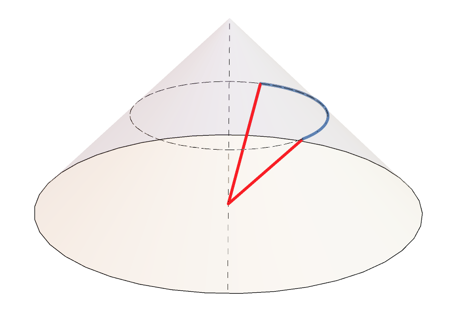
We focus on entangling regions that lie on the slice $u=0$ as other configurations can be obtained by acting with bulk isometries. The entangling regions $A$ are given by patches on the sphere at infinity that are invariant under the flow. They are "watermelon slices" whose boundaries follow the flow and with width $\ell_{\phi}$ . They can be parametrized as

-\tfrac{\ell_{\phi}}{2}\leq\phi\leq\tfrac{\ell_{\phi}}{2},\qquad 0\leq\theta\leq\pi\,,

(141)

and are represented in Fig. 5. The domain of dependence $\mathcal{D}$ and its boundary $\partial\mathcal{D}$ can be checked to be invariant under the flow.¹²¹² 12 The boundary $\partial A$ is not fixed pointwise by the flow, which is different from the AdS case or in 3d Minkowski. This is inevitable for 4d Minkowski because there is no conformal Killing on the sphere which admits a one-dimensional set of fixed points 2011JGP….61..589B.

Generalized Rindler transformations.

When the sphere is written in complex coordinates

z=e^{i\phi}\mathrm{cot}(\tfrac{\theta}{2}),\qquad\bar{z}=e^{-i\phi}\mathrm{cot}(\tfrac{\theta}{2})\,,

(142)

we observe that the Rindler transformation (136) can be written as

z\to e^{-w},\qquad\bar{z}\to e^{-\bar{w}},

(143)

where $w=\rho-i\eta,\,\bar{w}=\rho+i\eta$ . This suggests a way to obtain more general Rindler transformations, obtained by acting with a Möbius transformation on the sphere. Let’s consider the following transformation

$\displaystyle u$	$\displaystyle\rightarrow$	$\displaystyle{\mathrm{cos}\,\theta_{0}\over\mathrm{cosh}\,\rho\,+\mathrm{cos}\,\eta\,\mathrm{sin}\,\theta_{0}}\tau\penalty\ ,$	(144)
$\displaystyle z$	$\displaystyle\rightarrow$	$\displaystyle{\mathrm{sin}\,\theta_{0}+e^{w}(1+\mathrm{cos}\,\theta_{0})\over\mathrm{sin}\,\theta_{0}\,e^{w}+(1+\mathrm{cos}\,\theta_{0})},$
$\displaystyle\bar{z}$	$\displaystyle\rightarrow$	$\displaystyle{\mathrm{sin}\,\theta_{0}+e^{\bar{w}}(1+\mathrm{cos}\,\theta_{0})\over\mathrm{sin}\,\theta_{0}\,e^{\bar{w}}+(1+\mathrm{cos}\,\theta_{0})}\,,$

which is a BMS₄ transformation. The boundary modular flow is the vector $2\pi\partial_{\rho}$ given by

\zeta_{A}=-{2\pi\over\mathrm{cos}\,\theta_{0}}\left(u\,\mathrm{cos}\,\theta\,\partial_{u}+k\right)\,,

(145)

where $k$ is a conformal Killing of the sphere given by

k=(\mathrm{sin}\,\theta-\mathrm{sin}\,\theta_{0}\,\mathrm{cos}\,\phi)\,\partial_{\theta}+\mathrm{sin}\,\theta_{0}\,\mathrm{cot}\,\theta\,\mathrm{sin}\,\phi\,\partial_{\phi}\penalty\ .

(146)

The bulk modular flow is

\xi_{A}={2\pi\over\mathrm{cos}\,\theta_{0}}\left((u+r)\,\mathrm{cos}\,\theta\,\partial_{r}-{u\over r}\mathrm{sin}\,\theta\,\partial_{\theta}\right)+\zeta_{A}\,.

(147)

It is obtained as the Killing vector of 4d Minkowski spacetime which matches with $\zeta_{A}$ on the boundary. The transformation described in (144) has also the thermal identification $\rho\sim\rho+2\pi i$ . It is a one-parameter generalization of the previous Rindler transformation (143), obtained by considering a more general conformal Killing $k$ of the sphere.

Generalized watermelons.

To understand the entangling regions associated to this modular flow, we should look at regions on $S^{2}$ that are preserved under $k$ . There are two fixed points given by

P_{-}:(\theta,\phi)=(\theta_{0},0),\quad P_{+}:(\theta,\phi)=(\pi-\theta_{0},0)\,.

(148)

The vector field $k$ is a flow from $P_{-}$ to $P_{+}$ . The entangling regions are deformed "watermelons slices" whose boundaries are tangent to this flow, as depicted in Fig. 5. The domain of dependence $\mathcal{D}$ and its boundary $\partial\mathcal{D}$ can be checked to be invariant under the flow. An entangling region $A$ can be parametrized by

-\ell(\theta)\leq\phi\leq\ell(\theta),\qquad\theta_{0}\leq\theta\leq\pi-\theta_{0}\,,

(149)

where $\ell(\theta)$ satisfies the condition

\ell^{\prime}(\theta)=\left.({k^{\phi}/k^{\theta}})\right|_{\phi=\ell(\theta)}\,,

(150)

which ensures that the boundary $\partial A$ is tangent to the vector field $k$ . This makes sure that $A$ and $\partial A$ are preserved under the modular flow. Explicitly, we obtain

\mathrm{tan}\,\ell(\theta)={\mathrm{cos}(2\theta_{0})-\mathrm{cos}(2\theta)\over 2\,\mathrm{sin}\,\theta\,\left(\mathrm{cot}(\tfrac{\ell_{\phi}}{2})\,\mathrm{sin}\,\theta+\mathrm{sin}\,\theta_{0}\,\sqrt{1+\mathrm{cot}^{2}(\tfrac{\ell_{\phi}}{2})-{\mathrm{sin}^{2}\theta_{0}\over\mathrm{sin}^{2}\theta}}\right)}\,,

(151)

where $\ell_{\phi}$ parametrizes the width of the entangling region. For $\theta_{0}=0$ , we have $\ell(\theta)=\ell_{\phi}/2$ . At small $\ell_{\phi}$ , we have

\ell(\theta)=\left(1-{\mathrm{sin}\,\theta_{0}\over\mathrm{sin}\,\theta}\right)\,{\ell_{\phi}\over 2}+O(\ell_{\phi}^{2})\,.

(152)

At the special value $\ell_{\phi}={\pi\over 2}$ , the watermelon becomes a disk on the sphere. This is illustrated in Fig. 5. The opening angle of the disk is $\pi-2\theta_{0}$ .

Ryu-Takayanagi surfaces.

The entangling regions described above are the generalization of the 3d story with $\ell_{u}=0$ . The bulk modular flow (147) is very similar to the bulk modular flow in three dimensions (11). The RT surfaces associated to the above regions are easy to describe, they lie on the slice $u=0$ and are the union of all light rays starting at the origin and ending on $\partial A$ . We illustrate this prescription in Fig. 5 by representing the sphere at infinity on the slice $u=0$ . The entangling regions $A$ are in blue and the RT surfaces $\widetilde{A}$ are in red. We also represent the boundary modular flow on the sphere. The entanglement entropy of the region $A$ is then given by

S_{A}=\int_{\widetilde{A}}{\rm\textbf{Q}}[\xi_{A}]\penalty\ .

(153)

For Einstein gravity in the Minkowski vacuum, the areas of all these RT surfaces vanish because they have a null tangent vector everywhere.

Perturbations.

As an illustration, we can consider on-shell perturbations of 4d Minkowski in the Bondi gauge. The flat metric is given by

ds^{2}=-du^{2}-2dudr+r^{2}\gamma_{ij}dx^{i}dx^{j},\qquad\gamma_{ij}dx^{i}dx^{j}=d\theta^{2}+\mathrm{sin}^{2}\theta\,d\phi^{2}\,,

(154)

we consider the linearized on-shell perturbations studied in Campoleoni:2017qot with $C_{ij}=0$ , which corresponds to setting the gravitational wave aspect to zero. Asymptotically, the perturbation reads

h_{uu}={2\over r}\mathcal{M}(x^{i})+O(r^{-2}),\qquad h_{ui}={1\over r}\mathcal{N}_{i}(x^{i})+O(r^{-2}),\qquad h_{ij}=O(1)\,.

(155)

The subleading pieces in $r$ should not contribute to the charges at infinity. This allows us to compute $\delta E_{A}$ in a similar way as in the previous section. We obtain on a slice $u=0$

\delta E_{A}={3\over 8\,\mathrm{cos}\,\theta_{0}}\int_{A}d\theta d\phi\left[(\mathrm{cos}\,\phi\,\mathrm{sin}\,\theta_{0}-\mathrm{sin}\,\theta)\mathcal{N}_{\theta}(\theta,\phi)-\mathrm{cot}\,\theta\,\mathrm{sin}\,\phi\,\mathrm{sin}\,\theta_{0}\,\mathcal{N}_{\phi}(\theta,\phi)\right],

(156)

which can be written in terms of the boundary modular flow (145) as

\delta E_{A}={3\over 16\pi}\int_{A}d\theta d\phi\,\zeta_{A}^{i}\mathcal{N}_{i}(\theta,\phi)\,.

(157)

Exactly as in the 3d case, the entropy has to be computed using the refined prescription (49) where we regulate the corner of the RT surface. The fact that $\delta E_{A}=S_{A}$ , which has to be positive, gives some constraints on the perturbations that can be described by a quantum system on $\mathcal{I}^{+}$ satisfying our assumptions, similar to the discussion in Sec. 3.4. These constraints impose the functions $\mathcal{N}_{i}$ in the perturbation to be such that (157) is positive for a given region $A$ . This selects a subspace $\mathcal{H}_{\text{code}}$ on which $K_{A}$ is bounded from below and this makes the density operator $e^{-K_{A}}$ is well-defined.

6.2 General 4d prescription

In this section, we discuss the general RT prescription in 4d, in the same spirit as the 3d discussion of Sec. 3.2. Given a boundary entangling region, we will describe the most general choice of light sheaf that satisfies the requirements to give a good RT configuration. That is, the light sheaf must connect $\partial A$ to the Rindler bifurcation surface and the modular flow must be tangent to it. As explained in the 3d case, the first condition ensures that we can define an RT surface (as a portion of the Rindler bifurcation surface) and the second condition is required to have a well-defined first law.

Modular flow for non-zero $\ell_{u}$ .

In Cartesian coordinates $(t,x,y,z)$ , the bulk modular flow given (140) takes the following form

\xi_{A}={2\pi\over\mathrm{cos}\,\theta_{0}}\left[z\,\partial_{t}+z\,\mathrm{sin}\,\theta_{0}\,\partial_{x}+\left(t-x\,\mathrm{sin}\,\theta_{0}\right)\partial_{z}\right]\penalty\ .

(158)

We note that this it is similar to the 3d bulk modular flow at $\ell_{u}=0$ . This suggests the following generalization for $\ell_{u}\neq 0$ in 4d, obtained by performing a bulk translation

z\rightarrow z+{\ell_{u}\over 2\,\mathrm{cos}\,\theta_{0}}\penalty\ ,

(159)

which leads to

\xi_{A}={2\pi\over\mathrm{cos}\,\theta_{0}}\left[\left(z+{\ell_{u}\over 2\,\mathrm{cos}\,\theta_{0}}\right)\partial_{t}+\left(z\,\mathrm{sin}\,\theta_{0}\,+{\ell_{u}\,\mathrm{tan}\,\theta_{0}\over 2}\right)\partial_{x}+\left(t-x\,\mathrm{sin}\,\theta_{0}\right)\partial_{z}\right]\penalty\ .

(160)

Going back to Bondi coordinates $(u,r,\theta,\phi)$ and taking the limit $r\to+\infty$ , we obtain the corresponding 4d boundary modular flow, which reads

	$\displaystyle\zeta_{A}$	$\displaystyle=$	$\displaystyle{2\pi\over\mathrm{cos}\,\theta_{0}}\left[\left(-u\,\mathrm{cos}\,\theta+{\ell_{u}\over 2\,\mathrm{cos}\,\theta_{0}}\left(1-\mathrm{sin}\,\theta_{0}\,\mathrm{sin}\,\theta\,\mathrm{cos}\,\phi\right)\right)\partial_{u}\right.$		(161)
			$\displaystyle\hskip 42.67912pt\left.\vphantom{\ell_{u}\over 2\,\mathrm{cos}\,\theta_{0}}+\left(\mathrm{sin}\,\theta_{0}\,\mathrm{cos}\,\phi-\mathrm{sin}\,\theta\right)\partial_{\theta}+\mathrm{sin}\,\theta_{0}\,\mathrm{cot}\,\theta\,\mathrm{sin}\,\phi\,\partial_{\phi}\right]\penalty\ .$		(161)

One can check that this modular flow follows from a generalized Rindler transform, which is the previous Rindler transform (144) with a different transformation for $u$

$\displaystyle u$	$\displaystyle\rightarrow$	$\displaystyle{\mathrm{cos}\,\theta_{0}\over\mathrm{cosh}\,\rho\,+\mathrm{cos}\,\eta\,\mathrm{sin}\,\theta_{0}}\left(\tau+{\ell_{u}\over 2\,\mathrm{cos}\,\theta_{0}}\mathrm{sinh}\,\rho\right),$	(162)
$\displaystyle z$	$\displaystyle\rightarrow$	$\displaystyle{\mathrm{sin}\,\theta_{0}+e^{w}(1+\mathrm{cos}\,\theta_{0})\over\mathrm{sin}\,\theta_{0}\,e^{w}+(1+\mathrm{cos}\,\theta_{0})},$
$\displaystyle\bar{z}$	$\displaystyle\rightarrow$	$\displaystyle{\mathrm{sin}\,\theta_{0}+e^{\bar{w}}(1+\mathrm{cos}\,\theta_{0})\over\mathrm{sin}\,\theta_{0}\,e^{\bar{w}}+(1+\mathrm{cos}\,\theta_{0})}\,,$

and which remains a BMS₄ transformation. The generator of the thermal circle $2\pi\partial_{\rho}$ reproduces the boundary modular flow given above. This was guaranteed to work because, as in 3d, the case $\ell_{u}\neq 0$ is simply the image of the case $\ell_{u}=0$ by a bulk translation, which becomes on the boundary

u\rightarrow u+{\ell_{u}\over 2\,\mathrm{cos}\,\theta_{0}}\mathrm{cos}\,\theta\penalty\ .

(163)

On the boundary, this bulk translation changes the shape of the region $A$ which is the same as before but with an extension in $u$ :

u={\ell_{u}\over 2\,\mathrm{cos}\,\theta_{0}}\mathrm{cos}\,\theta\penalty\ ,\qquad\theta\in[\theta_{0},\pi-\theta_{0}]\penalty\ .

(164)

Similarly to 3d, the bulk modular flow (160) is simply a boost. This can be seen explicitly by defining new coordinates

\tilde{t}={1\over\mathrm{cos}\,\theta_{0}}t-\mathrm{tan}\,\theta_{0}\,x,\qquad\tilde{x}={1\over\mathrm{cos}\,\theta_{0}}\,x-\mathrm{tan}\,\theta_{0}\,t,\qquad\tilde{z}=z+{\ell_{u}\over 2\,\mathrm{cos}\,\theta_{0}}\penalty\ ,

(165)

in which the modular flows is given by

\xi_{A}=2\pi\left(\tilde{z}\,\partial_{\tilde{t}}+\tilde{t}\,\partial_{\tilde{z}}\right)\penalty\ .

(166)

In App. A we show that, exactly like in the 3d case, there exists a change of coordinates in the bulk defined on the exterior of a Rindler horizon that maps to the transformation (162) on the boundary.

RT prescription.

In 4d, the prescription where we impose that the light rays pass through the origin $r=0$ is inconsistent in the case $\ell_{u}\neq 0$ because most light rays won’t have an intersection with the bifurcation surface. Instead, we should consider the most general light sheaf which satisfies the requirements necessary for a good RT configuration, as was done in Sec. 3.2 for the 3d case. We will take all these choices of light sheaf to be equally physical, reflecting a choice of UV cutoff in the putative dual theory.

The boundary of $A$ on $\mathcal{I}^{+}$ has two pieces $\partial A=B_{+}\cup B_{-}$ which can be parametrized as

	$\displaystyle B_{+}$	$\displaystyle:\quad\phi=\ell(\theta),\qquad$	$\displaystyle\theta_{0}\leq\theta\leq\pi-\theta_{0}\penalty\ ,$		(167)
	$\displaystyle B_{-}$	$\displaystyle:\quad\phi=-\ell(\theta),\qquad$	$\displaystyle\theta_{0}\leq\theta\leq\pi-\theta_{0}\penalty\ .$

where $\ell(\theta)$ is defined in (151), while their extension in the $u-$ direction is given by (164). The most general light rays that arrive at a point $(\theta,\phi)=(\theta,\pm\ell(\theta))$ on $\mathcal{I}^{+}$ can be parametrized as follows in Cartesian coordinates

\gamma_{+}(\theta):\begin{cases}t=s+T_{+}(\theta)\\ x=s\,\mathrm{sin}\,\theta\,\mathrm{cos}\,\ell(\theta)+X_{+}(\theta)\\ y=s\,\mathrm{sin}\,\theta\,\mathrm{sin}\,\ell(\theta)+Y_{+}(\theta)\\ z=s\,\mathrm{cos}\,\theta+Z_{+}(\theta)\end{cases},\qquad\gamma_{-}(\theta):\begin{cases}t=s+T_{-}(\theta)\\ x=s\,\mathrm{sin}\,\theta\,\mathrm{cos}\,\ell(\theta)+X_{-}(\theta)\\ y=s\,\mathrm{sin}\,\theta\,\mathrm{sin}\,\ell(\theta)+Y_{-}(\theta)\\ z=s\,\mathrm{cos}\,\theta+Z_{-}(\theta)\end{cases}\penalty\ ,

(168)

and the arbitrary functions $T_{\pm}(\theta),X_{\pm}(\theta),Y_{\pm}(\theta),Z_{\pm}(\theta)$ reflect the ambiguity in choosing these light rays. This ambiguity will be partially fixed by imposing the necessary requirements. Firstly, the light rays $\gamma_{+}(\theta)$ and $\gamma_{-}(\theta)$ should intersect $\mathcal{I}^{+}$ at $\partial A$ , so that the value of $u$ at infinity is given by (164). Then we should impose that all these light rays intersect the bifurcation surface of the Rindler horizon associated with the bulk modular flow, i.e. $\tilde{t}=\tilde{z}=0$ . To do this, we impose that after transforming (168) to the new Cartesian coordinates (165), ${\tilde{z}}$ and ${\tilde{t}}$ become proportional. This also imposes the relation

{\tilde{z}}=f(\theta)\,{\tilde{t}},\qquad f(\theta)={\mathrm{cos}\,\theta\,\mathrm{cos}\,\theta_{0}\over 1-\mathrm{cos}\,\ell(\theta)\,\mathrm{sin}\,\theta\,\mathrm{tan}\,\theta_{0}}\penalty\ .

(169)

Denoting the two light sheafs

	$\displaystyle\gamma_{+}$	$\displaystyle=$	$\displaystyle\{\gamma_{+}(\theta)\mid\theta\in[\theta_{0},\pi-\theta_{0}]\}\penalty\ ,$		(170)
	$\displaystyle\gamma_{-}$	$\displaystyle=$	$\displaystyle\{\gamma_{-}(\theta)\mid\theta\in[\theta_{0},\pi-\theta_{0}]\}\penalty\ ,$

we see that $\gamma_{+}$ and $\gamma_{-}$ span over the quadrant ${\tilde{t}}\geq|{\tilde{z}}|$ because the function $f(\theta)$ is a bijection between the interval $[\theta_{0},\pi-\theta_{0}]$ and the interval $[-1,1]$ . To find the region $\gamma$ , which is a 2d surface in 4d, we should consider the intersection of $\gamma_{\pm}$ with the bifurcation surface, which is the plane $({\tilde{x}},{\tilde{y}})$ . From the explicit parametrization, we find that the intersection of $\gamma_{\pm}$ with this plane is restricted to the lines

{\tilde{x}}\pm\mathrm{cos}\,\theta_{0}\,\mathrm{tan}(\tfrac{\ell_{\phi}}{2})\,{\tilde{y}}=0\penalty\ .

(171)

Lastly, we should impose that the modular flow is tangent to the light sheaf $\gamma_{+}\cup\gamma_{-}$ which is required to have a well-defined first law. This is necessary because we need $\xi_{A}\cdot\Theta$ to vanish when integrated on the light sheaf, see the paragraph below for more details. To do this, we consider the two tangent vectors

{\partial x^{\mu}\over\partial\theta}\partial_{\mu},\qquad{\partial x^{\mu}\over\partial s}\partial_{\mu}\penalty\ ,

(172)

and we require that the modular flow $\xi_{A}$ can be written as a linear combination of those. For the light sheaf $\gamma_{+}$ , we find that this is only possible if the light sheaf $\gamma_{+}$ intersects the bifurcation surface at a single point $P_{+}$ . That is, we need all the light rays in $\gamma_{+}$ to converge to the same point $P_{+}$ on the bifurcation surface. We have a similar condition on $\gamma_{-}$ which should intersect the bifurcation surface at a single point $P_{-}$ . These points cannot be arbitrary in the plane $({\tilde{x}},{\tilde{y}})$ since they have to belong to the lines given in (171). Importantly, $P_{+}$ and $P_{-}$ don’t have to be the same. Enforcing all these constraints, we are able to fix the functions $T_{\pm}(\theta),X_{\pm}(\theta),Y_{\pm}(\theta),Z_{\pm}(\theta)$ and we can write the following simpler parametrization for the light sheafs

\displaystyle\gamma_{\pm}(\theta):\begin{cases}t=\mp\tilde{y}_{\pm}\,\mathrm{sin}\,\theta_{0}\,\mathrm{tan}(\tfrac{\ell_{\phi}}{2})+s,\\ x=\mp\tilde{y}_{\pm}\,\mathrm{tan}(\tfrac{\ell_{\phi}}{2})+s\,\mathrm{sin}\,\theta\,\mathrm{cos}\,\ell(\theta)\\ y=\tilde{y}_{\pm}\pm s\,\mathrm{sin}\,\theta\,\mathrm{sin}\,\ell(\theta)\\ z=-{\ell_{u}\over 2\,\mathrm{cos}\,\theta_{0}}+s\,\mathrm{cos}\,\theta\end{cases}.

(173)

In this parametrization, the light sheafs $\gamma_{\pm}$ intersect the bifurcation surface ${\tilde{t}}={\tilde{z}}=0$ at $P_{+}$ and $P_{-}$ whose coordinates are given by

P_{\pm}:\quad{\tilde{t}}={\tilde{z}}=0,\qquad{\tilde{y}}={\tilde{y}}_{\pm},\qquad{\tilde{x}}=\mp\mathrm{cos}\,\theta_{0}\,\mathrm{tan}(\tfrac{\ell_{\phi}}{2}){\tilde{y}}_{\pm}\penalty\ .

(174)

The simplest choice is to take $P_{-}=P_{+}$ . The RT configuration that we obtain is the one described in the previous section (up to a bulk isometry) and the RT surface has a conical shape. We can also have configurations where $P_{-}$ and $P_{+}$ are separated. In this case, we should add additional light rays to close the light sheaf. To do this, we define new light sheafs $\gamma_{N}$ and $\gamma_{S}$ consisting of light rays that go from the two poles of $\partial A$ given by

N:(\theta,\phi)=(\theta_{0},0),\qquad S:(\theta,\phi)=(\pi-\theta_{0},0)\penalty\ ,

(175)

and intersect the bifurcation surface. It turns out that it is possible to make such a light ray intersect an arbitrary point on the bifurcation surface. For example, a parametrization of $\gamma_{N}$ and $\gamma_{S}$ can be given as

\displaystyle\gamma_{N}(v):\begin{cases}{\tilde{t}}=s\,\mathrm{cos}\,\theta_{0},\\ {\tilde{x}}=X_{N}(v)\\ {\tilde{y}}=Y_{N}(v)\\ {\tilde{z}}=s\,\mathrm{cos}\,\theta_{0}\end{cases},\qquad\gamma_{S}(v):\begin{cases}{\tilde{t}}=s\,\mathrm{cos}\,\theta_{0},\\ {\tilde{x}}=X_{S}(v)\\ {\tilde{y}}=Y_{S}(v)\\ {\tilde{z}}=-s\,\mathrm{cos}\,\theta_{0}\penalty\ ,\end{cases}

(176)

where $v$ parametrizes the different light rays in the light sheafs $\gamma_{N}$ and $\gamma_{S}$ . These light sheafs satisfy our requirements: they intersect $\mathcal{I}_{+}$ at the two poles $N$ and $S$ (with the required value of $u$ ) and the bulk modular flow is tangent to them. The intersection of $\gamma_{N}$ with the bifurcation surface is at $s=0$ and gives a curve $C_{N}:({\tilde{x}},{\tilde{y}})=(X_{N}(v),Y_{N}(v))$ parametrized by $v$ . Similarly, $\gamma_{S}$ intersects the bifurcation surface at the curve $C_{S}:({\tilde{x}},{\tilde{y}})=(X_{S}(v),Y_{S}(v))$ . Both of those curves must connect $P_{+}$ to $P_{-}$ . The total light sheaf is given by $\gamma_{+}\cup\gamma_{N}\cup\gamma_{S}\cup\gamma_{-}$ . This configuration is illustrated in Fig. 6.

The surface $\gamma$ is the portion of the bifurcation surface which is in the interior of the contour formed by $C_{N}$ and $C_{S}$ . It is depicted in the plane $({\tilde{x}},{\tilde{y}})$ in Fig. 7. The RT surface $\widetilde{A}$ is the union of the total light sheaf with $\gamma$ . The entanglement entropy of $A$ is given by

S_{A}=\int_{\widetilde{A}}{\rm\textbf{Q}}[\xi_{A}]\penalty\ .

(177)

In Einstein gravity, the integration of Wald’s functional on the light sheaf vanishes so the entanglement entropy of $A$ is given by the area of the region $\gamma$

S_{A}={\mathrm{Area}(\gamma)\over 4G}\penalty\ .

(178)

The possible regions $\gamma$ can be obtained by the following procedure: put two points $P_{\pm}$ on the two lines (171) (depicted in grey in Fig. 7). Then, connect them by two arbitrary curves $C_{N}$ and $C_{S}$ so that their union has a well-defined interior. This interior is the region $\gamma$ and the entropy is given by the area of $\gamma$ (in Einstein gravity). We see that as in 3d, the entropy is sensitive to the choice of light sheaf, which should reflect a choice of UV cutoff in the putative dual field theory.

First law of entanglement.

We have the following definitions

\delta S_{A}=\int_{\widetilde{A}}\delta{\rm\textbf{Q}}[\xi_{A}],\qquad\delta E_{A}=\int_{A}{\bm{\chi}}\penalty\ ,

(179)

the first law states that these two expressions are equal on-shell. The 3d derivation of Sec. 3.3 can be carried out in 4d. In this derivation, the first law follows from the fact that

\int_{\widetilde{A}}\xi_{A}\cdot{\bm{\Theta}}[\delta g]=0\penalty\ ,

(180)

which holds whenever $\xi_{A}$ is tangent to $\widetilde{A}$ . This is the case here since $\xi_{A}$ vanishes on $\gamma$ and is tangent to the light sheaf (this was one of our requirements). As a result, all the RT surfaces described here satisfy a first law for perturbations.

6.3 Linearized gravitational equations

In this section, we prove that the four-dimensional linearized gravitational equations follow from the first law of entanglement. The proof is very similar to the three-dimensional case described in Sec. 4, to which we refer for more details.

Reference configuration.

We consider a watermelon $A$ at $u=0$ with $\ell_{u}=0$ . The first law of entanglement gives the equation

\int_{\theta_{0}}^{\pi-\theta_{0}}d\theta\int_{-\ell(\theta)}^{\ell(\theta)}d\phi\int_{0}^{+\infty}dr\,\xi^{a}\delta E_{ab}{\bm{\varepsilon}}^{b}=0\,,

(181)

where $\varepsilon_{a}={1\over 6}\varepsilon_{abcd}dx^{b}\wedge dx^{c}\wedge dx^{d}$ and $\ell(\theta)$ is defined in (151) and contains the parameter $\ell_{\phi}$ which parametrizes the width of $A$ . The dependence on $\ell_{\phi}$ enters in a complicated fashion. However, we can differentiate with respect to $\ell_{\phi}$ at $\ell_{\phi}=0$ , where we can use the expansion (152). This leads to

\int_{\theta_{0}}^{\pi-\theta_{0}}d\theta\left(1-{\mathrm{sin}\,\theta_{0}\over\mathrm{sin}\,\theta}\right)\int_{0}^{+\infty}dr\,\xi^{a}\delta E_{ab}{\bm{\varepsilon}}^{b}=0\,,

(182)

where the LHS is evaluated at $\phi=0$ . In Bondi coordinates, we have

{\bm{\varepsilon}}^{r}=-{\bm{\varepsilon}}_{u}=-r^{2}\mathrm{sin}\,\theta\,dr\wedge d\theta\wedge d\phi\,.

(183)

The bulk modular flow (147) evaluated at $u=0$ and $\phi=0$ is given by

\xi_{A}={2\pi\over\mathrm{cos}\,\theta_{0}}\left(r\,\mathrm{cos}\,\theta\,\partial_{r}-(\mathrm{sin}\,\theta-\mathrm{sin}\,\theta_{0})\,\partial_{\theta}\right)\,,

(184)

so the integral becomes

\displaystyle\hskip-28.45274pt0

\displaystyle=

\displaystyle\int_{\theta_{0}}^{\pi-\theta_{0}}d\theta\left(\mathrm{sin}\,\theta-\mathrm{sin}\,\theta_{0}\right)\int_{0}^{+\infty}dr\left(-r^{3}\mathrm{cos}\,\theta\,\delta E_{rr}+r^{2}(\mathrm{sin}\,\theta-\mathrm{sin}\,\theta_{0})\,\delta E_{r\theta}\right)\,.

(185)

The expansion around $\theta_{0}={\pi\over 2}$ implies that

\int_{0}^{+\infty}dr\left.\left(r^{3}\partial_{\theta}\delta E_{rr}+2\,r^{2}\delta E_{r\theta}\right)\right|_{(u,\theta,\phi)=(0,\tfrac{\pi}{2},0)}=0\penalty\ .

(186)

Rotations and time translations.

As in the 3d case, we can consider new configurations obtained by performing rotations. They are the same as the reference configuration but centered at $\phi=\phi_{0}$ . We can also consider a translation $u\rightarrow u+u_{0}$ in retarded time $u$ . The Jacobians of these transformations are the identity which implies that the expression (186) becomes

\int_{0}^{+\infty}dr\left.\left(r^{3}\partial_{\theta}\delta E_{rr}+2\,r^{2}\delta E_{r\theta}\right)\right|_{(u,\theta,\phi)=(u_{0},\tfrac{\pi}{2},\phi_{0})}=0\penalty\ ,

(187)

for any $u_{0}$ and $\phi_{0}$ .

light sheaf deformation.

We consider the same boundary region $A$ but with the more general configuration described in Sec. 6.2. For the proof, we consider the configuration depicted on the right of Fig. 7. We put $P_{+}$ at the origin and $P_{-}$ at a distance $\ell$ from $P_{+}$ on one of the axis and we connect them by the two curves $C_{N}$ and $C_{S}$ , as represented on the figure. The configuration is parametrized by the length $\ell$ of the segment $[P_{+}P_{-}]$ and the overture angle $\alpha$ at $P_{-}$ . The first law of entanglement gives

I(\alpha,\ell)=\int_{\Sigma(\alpha,\ell)}d{\bm{\chi}}=0\penalty\ ,

(188)

where $\Sigma$ , the interior of the RT surface, depends on these two parameters $\alpha$ and $\ell$ . Let’s denote by $n$ the vector normal to the segment $C_{S}$

n=\mathrm{cos}(\tfrac{\ell_{\phi}}{2})\partial_{\tilde{x}}+\mathrm{cos}\,\theta_{0}\,\mathrm{sin}(\tfrac{\ell_{\phi}}{2})\partial_{\tilde{y}}\penalty\ ,

(189)

Taking the derivative of (188) with respect to $\alpha$ and evaluating at $\alpha=0$ , we obtain

\int_{0}^{+\infty}ds\int_{0}^{\ell}dv\left(n\cdot d{\bm{\chi}}\right)=0\penalty\ ,

(190)

where we have used the fact that $\gamma_{N}$ (176) can be parametrized by $s$ and $v$ . The vector tangent to $C_{S}$ is given by

m=\mathrm{cos}(\tfrac{\ell_{\phi}}{2})\partial_{\tilde{y}}-\mathrm{cos}\,\theta_{0}\,\mathrm{sin}(\tfrac{\ell_{\phi}}{2})\partial_{\tilde{x}}\penalty\ .

(191)

We can now take the derivative with respect to $\ell$ and evaluate at $\ell=0$ .

\int_{0}^{+\infty}dr\,(m\cdot(n\cdot d{\bm{\chi}}))|_{(\theta,\phi)=(\theta_{0},0)}=0

(192)

We have reduced the integral to a light ray going from the origin to the point of $\partial A$ with $(\theta,\phi)=(\theta_{0},0)$ (and $u=0$ as we are considering a region $A$ with $\ell_{u}=0$ ). We can then go to Bondi coordinates. From the change of coordinates, we can compute

	$\displaystyle m$	$\displaystyle=$	$\displaystyle-\mathrm{sin}\,\theta_{0}\,\mathrm{sin}(\tfrac{\ell_{\phi}}{2})\,\partial_{r}-{\mathrm{cos}\,\theta_{0}\,\mathrm{sin}(\tfrac{\ell_{\phi}}{2})\over r}\partial_{\theta}+{\mathrm{cos}(\tfrac{\ell_{\phi}}{2})\over r\,\mathrm{sin}\,\theta_{0}}\partial_{\phi}\penalty\ ,$		(193)
	$\displaystyle n$	$\displaystyle=$	$\displaystyle\mathrm{cos}(\tfrac{\ell_{\phi}}{2})\,\mathrm{tan}\,\theta_{0}\,\partial_{r}+{\mathrm{cos}(\tfrac{\ell_{\phi}}{2})\over r}\partial_{\theta}+{\mathrm{cot}\,\theta_{0}\,\mathrm{sin}(\tfrac{\ell_{\phi}}{2})\over r}\partial_{\phi}\penalty\ ,$

when evaluated at $\theta=\theta_{0}$ and $\phi=0$ . In the definition (55) of $d{\bm{\chi}}$ , the non-trivial contribution comes from

{\bm{\varepsilon}}^{r}=-{\bm{\varepsilon}}_{u}=-r^{2}\,\mathrm{sin}\,\theta\,dr\wedge d\theta\wedge d\phi\penalty\ .

(194)

Hence, we obtain that

m\cdot(n\cdot d{\bm{\chi}})|_{\gamma_{N}}=2\left(1-\mathrm{sin}^{2}\theta_{0}\,\mathrm{sin}^{2}(\tfrac{\ell_{\phi}}{2})\right)\,\xi_{A}^{a}\delta E_{ar}dr\penalty\ .

(195)

The bulk modular flow at $(u,\theta,\phi)=(0,\theta_{0},0)$ is simply given by

\xi_{A}=2\pi r\,\partial_{r}

(196)

Hence, we obtain

\displaystyle\int_{0}^{+\infty}dr\,r\delta E_{rr}(0,r,\theta_{0},0)=0\penalty\ ,

(197)

As previously, we can act with rotations and time translations to show that we have

\displaystyle\int_{0}^{+\infty}dr\,r\delta E_{rr}(u_{0},r,\theta_{0},\phi_{0})=0\penalty\ ,

(198)

for arbitrary $u_{0},\theta_{0},\phi_{0}$ .

Radial translations.

Let’s consider a new configuration which is obtained by translating the reference configuration by a distance $r_{0}$ in the direction $(\theta_{0},\phi_{0})$ of the light ray on which (198) is integrated. In Cartesian coordinates, such a translation is given by

t\rightarrow t+r_{0},\qquad x\rightarrow x+r_{0}\,\mathrm{cos}\,\theta_{0}\,\mathrm{cos}\,\phi_{0},\qquad y\rightarrow y+r_{0}\,\mathrm{cos}\,\theta_{0}\,\mathrm{sin}\,\phi_{0},\qquad z\rightarrow z+r_{0}\,\mathrm{sin}\,\theta_{0}\penalty\ .

(199)

This leads to the new constraint

\int_{r_{0}}^{+\infty}dr\,(r-r_{0})\,\delta E_{rr}(u_{0},r,\theta_{0},\phi_{0})=0\penalty\ ,

(200)

where we have also performed the change of variable $r\to r-r_{0}$ in the integral. Taking two derivatives with respect to $r_{0}$ shows that

\delta E_{rr}(u_{0},r_{0},\theta_{0},\phi_{0})=0\penalty\ ,

(201)

for any value of $u_{0},r_{0},\theta_{0},\phi_{0}$ . From this, the equation (187) simplifies to

\int_{0}^{+\infty}dr\,r^{2}\,\delta E_{r\theta}(u_{0},r,\tfrac{\pi}{2},\phi_{0})=0\penalty\ .

(202)

We use the same radial translation on this equation to obtain the constraint

\int_{r_{0}}^{+\infty}dr\,{(r-r_{0})^{2}\over r}\delta E_{r\theta}(u_{0},r,\tfrac{\pi}{2},\phi_{0})\penalty\ .

(203)

Taking three derivatives with respect to $r_{0}$ implies that

\delta E_{r\theta}(u_{0},r_{0},\tfrac{\pi}{2},\phi_{0})=0\penalty\ ,

(204)

which is true for any value of $u_{0},r_{0},\phi_{0}$ .

Vanishing of $\delta E_{r\theta}$ everywhere.

The equation (204) at $\phi_{0}=0$ shows that $\delta E_{r\theta}$ vanishes on the semi-infinite line $L_{P}$ given by $(\theta,\phi)=(\tfrac{\pi}{2},0)$ . Let’s now consider rotations in the plane $(x,z)$ . Under such rotations, $L_{P}$ covers the full disk in the $y=0$ plane, shown in orange in Fig. 8. The Jacobian of this transformation, when evaluated at $\phi=0$ , is diagonal in Bondi coordinates because it simply corresponds to a shift in $\theta$ . It is given explicitly by

{\partial x^{a}\over\partial\tilde{x}^{b}}=\begin{pmatrix}1&&&\\ &1&&\\ &&1&\\ &&&\mathrm{cos}\,\alpha-\mathrm{cot}\,\theta\,\mathrm{sin}\,\alpha\end{pmatrix}\,,

(205)

so we obtain $\delta E_{r\theta}=0$ when evaluated on this disk. For any point on this disk, we can then consider a rotation in the $(x,y)$ -plane, whose Jacobian is the identity. This shows that $\delta E_{r\theta}=0$ vanishes everywhere inside the ball. This implies that

\delta E_{r\theta}=0\,,

(206)

everywhere in the bulk. This procedure is illustrated in Fig. 8.

Boosts and rotations.

We now act with boosts and rotations on the previous configurations to generate more constraints on $\delta E_{ab}$ . Transforming the equation $\delta E_{r\theta}=0$ under the infinitesimal $(x,z)$ -rotation, the $(t,y)$ -boost and the $(t,x)$ -boost, we obtain

\delta E_{r\phi}=\delta E_{\theta\phi}=\delta E_{rr}=0,\qquad\delta E_{\theta\theta}=-r^{2}\delta E_{ur}\,.

(207)

Then, the image of $\delta E_{\theta\phi}=0$ under the $(x,z)$ -rotation implies that

\delta E_{\phi\phi}=-r^{2}\mathrm{sin}^{2}\theta\,\delta E_{ur}\,.

(208)

Conservation equation.

As in 3d, we consider the conservation equation

\nabla_{a}(\delta E^{ab})=0\,,

(209)

which is always satisfied by the equations of motion. For $b=r$ , this implies that

\partial_{r}(\delta E_{ur})=0\,,

(210)

which leads to

\delta E_{ur}=C_{0}(u,\phi),\qquad\delta E_{\theta\theta}=-r^{2}C_{0}(u,\phi),\qquad\delta E_{\phi\phi}=-r^{2}\mathrm{sin}^{2}\theta\,C_{0}(u,\phi)\,.

(211)

We expect that an analysis similar to the 3d one in Sec. 5 can be performed in 4d and that it will lead to a trace condition and three conservation equations for the holographic stress tensor in 4d Minkowski. A proof of this statement will require a detailed analysis of the flat limit of perturbed AdS₄ in Bondi gauge, which we leave for future work. From now on, we will assume that these boundary conditions ensure the vanishing of the components $\delta E_{ua}$ at leading asymptotic order. The trace condition, similar to (125) and (126) in 3d, should imply that $C_{0}=0$ , leading to

\delta E_{ur}=\delta E_{\theta\theta}=\delta E_{\phi\phi}=0\,,

(212)

everywhere in the bulk. The conservation equation (209) for $b=\theta,\phi$ gives

\partial_{r}(\delta E_{u\theta})+{2\over r}\delta E_{u\theta}=0,\qquad\partial_{r}(\delta E_{u\phi})+{2\over r}\delta E_{u\phi}=0\,.

(213)

The solutions of these equations are

\delta E_{u\theta}={C_{1}(u,\theta)\over r^{2}},\qquad\delta E_{u\phi}={C_{2}(u,\phi)\over r^{2}}\,.

(214)

We expect that the conservation of the boundary stress tensor implies that $C_{1}=C_{2}=0$ , leading to $\delta E_{u\theta}=\delta E_{u\phi}=0$ . Finally, the conservation equation (209) for $b=u$ gives

\partial_{r}(\delta E_{uu})+{2\over r}\delta E_{uu}=0\,.

(215)

which is solved by

\delta E_{uu}={C_{3}(u,\phi)\over r^{2}}\,,

(216)

and $C_{3}=0$ is expected to follow from the conservation of the boundary stress tensor. Thus, we have shown that all the components of the linearized gravitational equation vanish.

7 Conclusion

In this paper, we have considered holographic entanglement entropy in asymptotically flat spacetimes. Under some general assumptions on the dual field theory, an analog of the Ryu-Takayanagi formula was obtained in Jiang:2017ecm to compute the entanglement entropies of 3d Minkowski spacetime. We have refined and generalized this prescription and showed that it satisfies a first law when perturbations are considered. Using this RT prescription, we have shown that the first law of entanglement is equivalent to the linearized gravitational equations of motion. We have also extended all these results to 4d.

This result could have also been phrased purely in classical gravity, although it is natural to motivate it from the perspective of holography. It will be important to understand better the dual field theory, and try to prove the assumptions detailed in Sec. 2. Some recent progress in this direction include Barnich:2014kra; Oblak:2015sea; Campoleoni:2016vsh; Oblak:2016eij; Bagchi:2019xfx; Ball:2019atb; Himwich:2019dug; Donnay:2018neh; Hijano:2018nhq; Hijano:2019qmi.

Another line of research would be to push further the consequences of the RT prescription described here. One could hope to get some hints on the microscopic definition of the dual field theory, or show that one of the assumptions was incorrect. An important feature of our analysis is the importance of the choice of an infalling light sheaf. We believe that this is a hint towards the UV structure of the dual theory, which we hope to investigate in future work. The RT formula in AdS has given rise to a wealth of results connecting quantum information to the emergence of spacetime. It would be interesting to investigate these ideas in asymptotically flat spacetimes, using the RT prescription described here.

Acknowledgments

It is a pleasure to thank Jan de Boer, Samuel Gu erin, Hongliang Jiang, Erik Mefford, Kevin Morand, Romain Ruzziconi and Wei Song for useful discussions. We are grateful for the hospitality of Sylvia and Melba Huang and to the 2019 Amsterdam string theory summer workshop where this work was completed. This work was supported in part by the $\Delta$ -ITP consortium, a program of the NWO that is funded by the Dutch Ministry of Education, Culture and Science (OCW) and the ANR-16-CE31-0004 contract Black-dS-String.

Appendix A Bulk Rindler transformation

In this appendix, we describe the bulk extension of the generalized Rindler transform (7) on the boundary. The image of Minkowski spacetime under this bulk transformation turns out to be the upper wedge of a Rindler spacetime.

Bulk Rindler transformation in 3d.

We describe the change of coordinates that brings the metric in Bondi coordinates to the upper wedge of a Rindler spacetime. The Cartesian coordinates are related to Bondi coordinates using

t=u+r,\qquad x=r\,\mathrm{cos}\,\phi,\qquad y=r\,\mathrm{sin}\,\phi,

(217)

and the coordinates in which the modular flow is a boost are

\tilde{t}={t\over\mathrm{sin}(\tfrac{\ell_{\phi}}{2})}-\mathrm{cot}(\tfrac{\ell_{\phi}}{2})\,x,\qquad\tilde{x}={x\over\mathrm{sin}(\tfrac{\ell_{\phi}}{2})}-\mathrm{cot}(\tfrac{\ell_{\phi}}{2})\,t,\qquad\tilde{y}=y+{\ell_{u}\over 2\,\mathrm{sin}(\tfrac{\ell_{\phi}}{2})}.

(218)

We define new coordinates $(\tilde{\tau},\rho)$ satisfying

\tilde{t}=e^{\tilde{\tau}}\mathrm{cosh}\,\rho,\quad\tilde{y}=e^{\tilde{\tau}}\mathrm{sinh}\,\rho.

(219)

These coordinates only cover the upper wedge $\tilde{t}^{2}-\tilde{y}^{2}>0$ . In these coordinates the bulk metric and modular flow are given by

\xi_{A}=2\pi\partial_{\rho},\quad ds^{2}=e^{2\tilde{\tau}}(-d\tilde{\tau}^{2}+d\rho^{2})+d\tilde{x}^{2}.

(220)

We recognize the Rindler metric and the bulk modular flow generates the (spacelike) Rindler evolution. The Rindler horizon is situated at $\tilde{\tau}=-\infty$ . To obtain the bulk extension of the generalized Rindler transform, consider the new coordinates $\{\tau,\tilde{x},\rho\}$ satisfying

\tau=e^{\tilde{\tau}}-\tilde{x},

(221)

defined only for $\tau>-\tilde{x}$ . The metric becomes

ds^{2}=-d\tau^{2}-2d\tau d\tilde{x}+(\tau+\tilde{x})^{2}d\rho^{2},

(222)

and the bulk modular flow is still $\xi_{A}=2\pi\partial_{\rho}$ . The Rindler horizon is at $\tau=-\tilde{x}$ . Finally, the bulk transformation is obtained by writing the new coordinates in terms of Bondi coordinates $\{u,r,\phi\}$ :

$\displaystyle\tau$	$\displaystyle=$	$\displaystyle-\tilde{x}+\left[{1\over\mathrm{sin}^{2}(\tfrac{\ell_{\phi}}{2})}\left(r+u-r\,\mathrm{cos}\left(\frac{\ell_{\phi}}{2}\right)\mathrm{cos}\,\phi\,\right)^{2}-\frac{1}{4}\left({\ell_{u}\over\,\mathrm{sin}(\tfrac{\ell_{\phi}}{2})}+2r\,\mathrm{sin}\,\phi\,\right)^{2}\right]^{1/2},$
$\displaystyle\tilde{x}$	$\displaystyle=$	$\displaystyle\frac{r\,\mathrm{cos}\,\phi}{\mathrm{sin}(\tfrac{\ell_{\phi}}{2})}-\mathrm{cot}(\tfrac{\ell_{\phi}}{2})\,(r+u),$
$\displaystyle\rho$	$\displaystyle=$	$\displaystyle\text{arccoth}\left(\frac{r+u-r\,\mathrm{cos}(\tfrac{\ell_{\phi}}{2})\,\mathrm{cos}\,\phi}{{\ell_{u}\over 2}+r\,\mathrm{sin}(\tfrac{\ell_{\phi}}{2})\,\mathrm{sin}\,\phi}\right).$	(223)

This coordinate system allows us to perform an asymptotic limit $r\rightarrow\infty$ , which gives

	$\displaystyle\tau$	$\displaystyle=$	$\displaystyle\frac{2u\,\mathrm{sin}(\tfrac{\ell_{\phi}}{2})-\ell_{u}\,\mathrm{sin}\,\phi}{2\,\mathrm{cos}\,\phi-2\,\mathrm{cos}(\tfrac{\ell_{\phi}}{2})},$		(224)
	$\displaystyle\rho$	$\displaystyle=$	$\displaystyle\text{arccoth}\left(\frac{1-\mathrm{cos}(\tfrac{\ell_{\phi}}{2})\,\mathrm{cos}\,\phi}{\mathrm{sin}(\tfrac{\ell_{\phi}}{2})\,\mathrm{sin}\,\phi}\right).$		(225)

One can check that this is exactly the inverse of the boundary generalized Rindler transformation (7), reproduced below

	$\displaystyle u$	$\displaystyle=$	$\displaystyle{\mathrm{sin}(\tfrac{\ell_{\phi}}{2})\,\over\mathrm{cosh}\,\rho+\mathrm{cos}(\tfrac{\ell_{\phi}}{2})}\left(\tau+\frac{\ell_{u}}{2\,\mathrm{sin}(\frac{\ell_{\phi}}{2})}\mathrm{sinh}\rho\right)\,,$		(226)
	$\displaystyle\phi$	$\displaystyle=$	$\displaystyle\mathrm{arctan}\left({\mathrm{sin}(\tfrac{\ell_{\phi}}{2})\,\mathrm{sinh}\,\rho\over 1+\mathrm{cos}(\tfrac{\ell_{\phi}}{2})\,\mathrm{cosh}\,\rho}\right)\,.$

Bulk Rindler transformation in 4d.

The same procedure can be carried out in 4d. Again, consider the bulk transformation from Bondi coordinates to Rindler coordinates in the upper wedge:

t=u+r,\quad x=r\,\mathrm{sin}\,\theta\,\mathrm{cos}\,\phi,\quad y=r\,\mathrm{sin}\,\theta\,\mathrm{sin}\,\phi,\quad z=r\,\mathrm{cos}\,\theta,

(227)

followed by

\tilde{t}=\frac{t}{\mathrm{cos}\,\theta_{0}}-\mathrm{tan}\,\theta_{0}\,x,\quad\tilde{x}=\frac{x}{\mathrm{cos}\,\theta_{0}}-\mathrm{tan}\,\theta_{0}\,t,\quad\tilde{y}=y,\quad\tilde{z}=z+\frac{\ell_{u}}{2\,\mathrm{cos}\,\theta_{0}},

(228)

and then

\tilde{t}=e^{\tilde{\tau}}\mathrm{cosh}\,\rho,\quad\tilde{z}=e^{\tilde{\tau}}\mathrm{sinh}\,\rho,\quad\tilde{x}=\mu\,\mathrm{cos}\,\eta,\quad\tilde{y}=\mu\,\mathrm{sin}\,\eta,

(229)

where the last two spacelike coordinates are mapped to polar coordinates: $\mu\in[0,\infty[$ and $\eta\in[0,2\pi[$ . In these coordinates, the metric and the bulk modular flow become

\xi_{A}=2\pi\partial_{\rho},\quad ds^{2}=e^{2\tilde{\tau}}(-d\tilde{\tau}^{2}+d\rho^{2})+d\mu^{2}+\mu^{2}d\eta^{2}.

(230)

Exactly like in 3d, we recognize the Rindler metric and the bulk modular flow generates the (spacelike) Rindler evolution. The Rindler horizon is at $\tilde{\tau}=-\infty$ . To obtain the bulk extension of the boundary generalized Rindler transform, we consider the new coordinates $\{\tau,\mu,\rho,\eta\}$ , such that

\tau=e^{\tilde{\tau}}-\mu,

(231)

defined only for $\tau>-\mu$ . The metric becomes

ds^{2}=-d\tau^{2}-2d\tau d\mu+(\tau+\mu)^{2}d\rho^{2}+\mu^{2}d\eta^{2},

(232)

while the bulk modular flow is still given by $\xi_{A}=2\pi\partial_{\rho}$ . The new radial coordinate is $\mu$ and by taking the limit $\mu\rightarrow\infty$ we confirm that the boundary metric is indeed the degenerate flat metric $d\rho^{2}+d\eta^{2}$ . The Rindler horizon is at $\tau=-\mu$ . Finally, the bulk transformation is obtained by writing the new coordinates in Bondi coordinates:

$\displaystyle\tau$	$\displaystyle=$	$\displaystyle\sqrt{\left(\frac{r+u}{\mathrm{cos}\,\theta_{0}}-r\,\mathrm{sin}\,\theta\,\mathrm{tan}\,\theta_{0}\,\mathrm{cos}\,\phi\right)^{2}-\frac{1}{4}\left(\frac{\ell_{u}}{\mathrm{cos}\,\theta_{0}}+2r\,\mathrm{cos}\,\theta\right)^{2}}$	(234)
		$\displaystyle-\sqrt{r^{2}\,\mathrm{sin}^{2}\theta\,\mathrm{sin}^{2}\phi+\left(\frac{r\,\mathrm{sin}\,\theta\,\mathrm{cos}\,\phi}{\mathrm{cos}\,\theta_{0}}-\mathrm{tan}\,\theta_{0}\,(r+u)\right)^{2}},$	(234)
$\displaystyle\mu$	$\displaystyle=$	$\displaystyle\sqrt{r^{2}\,\mathrm{sin}^{2}\theta\,\mathrm{sin}^{2}\phi+\left(\frac{r\,\mathrm{sin}\,\theta\,\mathrm{cos}\,\phi}{\mathrm{cos}\,\theta_{0}}-\mathrm{tan}\,\theta_{0}\,(r+u)\right)^{2}},$	(235)
$\displaystyle\rho$	$\displaystyle=$	$\displaystyle\text{arctanh}\left(\frac{{\ell_{u}\over 2}+r\,\mathrm{cos}\,\theta_{0}\,\mathrm{cos}\,\theta}{(r+u)-r\,\mathrm{sin}\,\theta_{0}\,\mathrm{sin}\,\theta\,\mathrm{cos}\,\phi}\right),$	(236)
$\displaystyle\eta$	$\displaystyle=$	$\displaystyle\text{arctan}\left(\frac{r\,\mathrm{cos}\,\theta_{0}\,\mathrm{sin}\,\theta\,\mathrm{sin}\,\phi}{r\,\mathrm{sin}\,\theta\,\mathrm{cos}\,\phi-\mathrm{sin}\,\theta_{0}\,(r+u)}\right).$	(237)

This allows us to perform the asymptotic limit $r\rightarrow\infty$ which gives

$\displaystyle\tau$	$\displaystyle=$	$\displaystyle{u\,\mathrm{cos}\,\theta_{0}-{\ell_{u}\over 2}\,\mathrm{cos}\,\theta\over\sqrt{(\mathrm{sin}\,\theta_{0}\,\mathrm{sin}\,\theta\,\mathrm{cos}\,\phi-1)^{2}-\mathrm{cos}^{2}\theta_{0}\,\mathrm{cos}^{2}\theta}}\penalty\ ,$	(238)
$\displaystyle\rho$	$\displaystyle=$	$\displaystyle\mathrm{arctanh}\left({\mathrm{cos}\,\theta_{0}\,\mathrm{cos}\,\theta\over 1-\mathrm{sin}\,\theta_{0}\,\mathrm{sin}\,\theta\,\mathrm{cos}\,\phi}\right)\penalty\ ,$	(239)
$\displaystyle\eta$	$\displaystyle=$	$\displaystyle\mathrm{arctan}\left({\mathrm{cos}\,\theta_{0}\,\mathrm{sin}\,\theta\,\mathrm{sin}\,\phi\over\mathrm{sin}\,\theta\,\mathrm{cos}\,\phi-\mathrm{sin}\,\theta_{0}}\right)\penalty\ .$

One can check that this is precisely the inverse of the boundary generalized Rindler transformation (162), reproduced below

$\displaystyle u$	$\displaystyle\rightarrow$	$\displaystyle{\mathrm{cos}\,\theta_{0}\over\mathrm{cosh}\,\rho\,+\mathrm{cos}\,\eta\,\mathrm{sin}\,\theta_{0}}\left(\tau+{\ell_{u}\over 2\,\mathrm{cos}\,\theta_{0}}\mathrm{sinh}\,\rho\right),$	(240)
$\displaystyle z$	$\displaystyle\rightarrow$	$\displaystyle{\mathrm{sin}\,\theta_{0}+e^{w}(1+\mathrm{cos}\,\theta_{0})\over\mathrm{sin}\,\theta_{0}\,e^{w}+(1+\mathrm{cos}\,\theta_{0})},$
$\displaystyle\bar{z}$	$\displaystyle\rightarrow$	$\displaystyle{\mathrm{sin}\,\theta_{0}+e^{\bar{w}}(1+\mathrm{cos}\,\theta_{0})\over\mathrm{sin}\,\theta_{0}\,e^{\bar{w}}+(1+\mathrm{cos}\,\theta_{0})}\,,$

where $z=e^{i\phi}\cot(\frac{\theta}{2})$ and $w=\rho-i\eta$ .

Appendix B Precisions on the general strategy

In this appendix, we make precise the general strategy explained in Sec. 4.1. Let $g:M\rightarrow M$ be a bulk isometry, $i:\Sigma\rightarrow M$ the original RT surface and $i_{g}=g\circ i:\Sigma\rightarrow M$ the image of this surface through isometry. The original RT surface is associated to a bulk modular flow $\xi$ to which corresponds a two-form $d{\bm{\chi}}[\xi]$ . The pullback of this two-form on $\Sigma$ is

\displaystyle i^{*}(d{\bm{\chi}}[\xi])=\xi^{a}(i(\sigma))\delta E_{ab}(i(\sigma))\frac{1}{2}\varepsilon^{b}_{cd}(i(\sigma))\frac{\partial x^{c}}{\partial\sigma^{\alpha}}\frac{\partial x^{d}}{\partial\sigma^{\beta}}d\sigma^{\alpha}\wedge d\sigma^{\beta},

(241)

where $\sigma$ stands for the coordinates on the two-dimensional manifold $\Sigma$ . Suppose that from the vanishing of the integral of this two-form on $\Sigma$ , we have been able to derive that some functional of $\delta E_{ab}$ vanishes at $i(\sigma)$ ,

\mathcal{F}\left[\delta E_{ab}(i(\sigma))\right]=0\penalty\ ,

(242)

for some $\bar{a},\bar{b}$ . We can now consider another surface, $(g\circ i)(\Sigma)$ in $M$ and we call its associated bulk modular flow $\xi_{g}$ . We should consider the pullback on the corresponding two-form $d{\bm{\chi}}[\xi_{g}]$ because

\displaystyle\int_{(g\,\circ\,i)(\Sigma)}d{\bm{\chi}}[\xi_{g}]=\int_{\Sigma}i^{*}_{g}d{\bm{\chi}}[\xi_{g}]\penalty\ .

(243)

The pullback is given by

i^{*}_{g}(d{\bm{\chi}}[\xi_{g}])=\xi_{g}^{a}(g\circ i(\sigma))\delta E_{ab}(g\circ i(\sigma))\frac{1}{2}\varepsilon^{b}_{cd}(g\circ i(\sigma))\frac{\partial g^{c}}{\partial x^{e}}\frac{\partial g^{d}}{\partial x^{f}}\frac{\partial x^{e}}{\partial\sigma^{\alpha}}\frac{\partial x^{f}}{\partial\sigma^{\beta}}d\sigma^{\alpha}\wedge d\sigma^{\beta}.

(244)

Now we can insert the identity matrix $\delta^{a}_{b}=\frac{\partial g^{a}}{\partial x^{c}}\frac{\partial x^{c}}{\partial g^{b}}$ to impose the equality of two $b$ -index, leading to

	$\displaystyle i^{*}_{g}(d{\bm{\chi}}[\xi_{g}])$	$\displaystyle=$	$\displaystyle\xi_{g}^{a}(g\circ i(\sigma))\delta E_{ab}(g\circ i(\sigma))\frac{\partial g^{b}}{\partial x^{g}}\left(\frac{\partial x^{g}}{\partial g^{h}}\frac{1}{2}\varepsilon^{h}_{cd}(g\circ i(\sigma))\frac{\partial g^{c}}{\partial x^{e}}\frac{\partial g^{d}}{\partial x^{f}}\right)$		(245)
			$\displaystyle\times\frac{\partial x^{e}}{\partial\sigma^{\alpha}}\frac{\partial x^{f}}{\partial\sigma^{\beta}}d\sigma^{\alpha}\wedge d\sigma^{\beta}.$		(245)

Now we can use the fact that $g$ is an isometry, while $\varepsilon^{h}_{cd}$ is the volume form to obtain than the parenthesis is actually $\frac{1}{2}\varepsilon^{g}_{ef}(i(\sigma))$ . Moreover we know that the modular flow for the image surface is the image of the modular flow of the initial surface under the $g$ -transformation: $\xi_{g}^{a}(g\circ i(\sigma))=\frac{\partial g^{a}}{\partial x^{b}}\xi^{b}(i(\sigma))$ . Finally, we obtain

i^{*}_{g}(d{\bm{\chi}}[\xi_{g}])=\xi^{i}(i(\sigma))\left(\frac{\partial g^{a}}{\partial x^{i}}\frac{\partial g^{b}}{\partial x^{g}}\delta E_{ab}(g\circ i(\sigma))\right)\frac{1}{2}\varepsilon^{g}_{ef}(i(\sigma))\frac{\partial x^{e}}{\partial\sigma^{\alpha}}\frac{\partial x^{f}}{\partial\sigma^{\beta}}d\sigma^{\alpha}\wedge d\sigma^{\beta},

(246)

which, is exactly (241) with the replacement

\delta E_{ab}(i(\sigma))\rightarrow\frac{\partial g^{c}}{\partial x^{a}}\frac{\partial g^{d}}{\partial x^{b}}\delta E_{cd}(g\circ i(\sigma))\penalty\ ,

(247)

which implies that (242) ensures that

\displaystyle\mathcal{F}\left[\frac{\partial g^{c}}{\partial x^{a}}\frac{\partial g^{d}}{\partial x^{b}}\delta E_{cd}(g\circ i(\sigma))\right]=0\,.

(248)

For example, if we can show that some components of $\delta E_{ab}$ vanish using a set of RT surfaces, we immediately obtain that other components, obtained by applying bulk isometries according to (248), will also vanish.

Appendix C Alternative proof in 3d

In this appendix, we provide an alternative to the step in the 3d proof of Sec. 4.2 where we used the light sheaf deformation. Here, we insist on doing this step using only RT configurations where the light rays $\gamma_{+}$ and $\gamma_{-}$ pass through the spatial origin $r=0$ . We will consider such configurations with $\ell_{u}\neq 0$ described in (3.1) which is the prescription used in Jiang:2017ecm. Although a better and equivalent¹³¹³ 13 This is because all the configurations described in Sec. 3.2 can be transformed with a bulk translation to a configuration where the two light rays pass through the line $r=0$ . derivation is presented in the main text, it is instructive to perform this step as presented here.

We should note that if we consider only the surfaces with $\ell_{u}=0$ (and with light rays passing through $r=0$ ), together with their image under bulk isometries, then the first law does not imply the gravitational equations: these surfaces don’t provide enough constraints. Indeed, the only constraint that we obtain is

\delta E_{r\phi}+r\partial_{r}\delta E_{r\phi}-r\partial_{\phi}\delta E_{rr}=0\penalty\ ,

(249)

and its image under bulk isometries. This does not imply that $\delta E_{ab}=0$ as it’s possible to find explicit counterexamples.

Hence, we need to consider RT surfaces with $\ell_{u}\neq 0$ (still requiring that the light rays pass through $r=0$ ). The computation becomes simpler in the limit of small $\ell_{u}$ . More precisely, we consider

\ell_{u}=\lambda\,\varepsilon^{2},\qquad\ell_{\phi}=\varepsilon\penalty\ ,

(250)

where we take $\varepsilon$ to be small. We would like to compute

I=\int_{\Sigma}\xi^{a}\delta E_{ab}{\bm{\varepsilon}}^{b}

(251)

in an expansion around $\varepsilon=0$ . The first law of entanglement will constrain $\delta E_{ab}$ to be such that $I=0$ . It turns out that $\lim_{\varepsilon\to 0}I=0$ for any perturbation, so we don’t get any constraint at zero order in $\varepsilon$ . To compute $I$ at first order in $\varepsilon$ , it is enough to consider the surface $\Sigma$ at first order in $\varepsilon$ ¹⁴¹⁴ 14 This can be justified as follows. Denoting $i_{\varepsilon}:S\rightarrow M$ the embedding of $\Sigma_{\varepsilon}$ in $M$ , we have $I=\int_{\Sigma_{\varepsilon}}\xi_{\varepsilon}^{a}\delta E_{ab}{\bm{\varepsilon}}^{b}={1\over 2}\int_{S}\xi_{\varepsilon}^{a}(i_{\varepsilon}(\sigma))\delta E_{ab}(i_{\varepsilon}(\sigma))\varepsilon_{cd}^{b}(i_{\varepsilon}(\sigma))(J_{\varepsilon})^{c}_{\penalty\ \alpha}(J_{\varepsilon})^{d}_{\penalty\ \beta}d\sigma^{\alpha}\wedge d\sigma^{\beta}\,$ (252) where $(J_{\varepsilon})^{c}_{\penalty\ \alpha}$ is the Jacobian of the embedding. This shows that, to compute the leading non-trivial term of $I$ , it is enough to take $i_{\varepsilon}$ at first order in $\varepsilon$ , which corresponds to taking the surface $\Sigma_{\varepsilon}$ at first order in $\varepsilon$ .. The configuration simplifies because the points $B_{+}$ and $B_{-}$ are at $u=O(\varepsilon^{2})$ . Hence, we have

B_{+}:\quad(u,\phi)=\left(0,{\varepsilon\over 2}\right),\qquad B_{-}:\quad(u,\phi)=\left(0,-{\varepsilon\over 2}\right)\penalty\ ,

(253)

to first order in $\varepsilon$ . We also have the following parametrization for the light rays

	$\displaystyle\gamma_{+}$		$\displaystyle:\quad(t,x,y)=\left(-2\eta+s,-2\eta+s,{\varepsilon\over 2}(-2\eta+s)\right),\qquad s\geq 0$		(254)
	$\displaystyle\gamma_{-}$		$\displaystyle:\quad(t,x,y)=\left(2\eta+s,2\eta+s,-{\varepsilon\over 2}(2\eta+s)\right),\qquad s\geq 0\penalty\ ,$

where we only kept the terms at first order in $\varepsilon$ . The curve $\gamma$ is simply a straight line connecting the two points

P_{+}:\quad(t,x,y)=(-2\eta,-2\eta,-\eta\epsilon),\quad P_{-}:\quad(t,x,y)=(2\eta,2\eta,-\eta\epsilon).

(255)

We can show that $\gamma_{-}$ stays at $u=0$ everywhere and that $\gamma_{+}$ is at $u=0$ for $s\geq 2\eta$ , which corresponds to all its points before it crosses the origin. Let’s call $\tilde{\gamma}_{-}$ the segment that connects the origin to $P_{-}$ , which , which is in the continuation of $\gamma_{-}$ past $P_{-}$ . The plane surface bounded by $\gamma_{-},\tilde{\gamma}_{-}$ and $\gamma_{+}$ (up to the origin) lies on the constant slice $u=0$ . It has the same shape as the RT surface for $\ell_{u}=0$ depicted in Fig. 1.

The additional piece consists in another triangle, bounded by $\gamma$ , $\tilde{\gamma}_{-}$ and $\tilde{\gamma}_{+}$ , where $\tilde{\gamma}_{+}$ is the piece of $\gamma_{+}$ connecting the origin to $P_{+}$ . This is the triangle $T=P_{-}P_{+}O$ . Let’s introduce coordinates

x_{+}=t+x,\qquad x_{-}=t-x

(256)

In these coordinates, we have (at first order)

	$\displaystyle P_{+}$		$\displaystyle:\quad(x_{+},x_{-},y)=(-4\lambda,0,-\lambda\varepsilon)$		(257)
	$\displaystyle P_{-}$		$\displaystyle:\quad(x_{+},x_{-},y)=(4\lambda,0,-\lambda\varepsilon)$

We see that the triangle $T=P_{+}P_{-}O$ can be parametrized as follows

x_{-}=0,\qquad-\lambda\varepsilon\leq y\leq 0,\qquad|x_{+}|\leq-{4y\over\varepsilon}

(258)

The integration over the triangle is

I=\int_{-\lambda\varepsilon}^{0}dy\int_{4y/\varepsilon}^{-4y/\varepsilon}dx_{+}\,F(x_{+},x_{-},y)\penalty\ ,

(259)

where $F$ is the appropriate integrand. We can redefine $y=\eta\varepsilon\tilde{y}$ so that it becomes

I=\lambda\varepsilon\int_{-1}^{0}d\tilde{y}\int_{4\lambda\tilde{y}}^{-4\lambda\tilde{y}}dx_{+}F(x_{+},x_{-},\lambda\varepsilon y)\penalty\ .

(260)

We now come back to the full integral

I=\int_{\Sigma}\xi^{a}\delta E_{ab}{\bm{\varepsilon}^{b}}\,,

(261)

which we want to evaluate at first order in $\varepsilon$ . The integral splits in an integral over the pizza slice and an integral over the triangle

I=I_{P}+I_{T}\penalty\ .

(262)

The integral over the pizza slice is

\displaystyle I_{P}

\displaystyle=

\displaystyle\int_{-\varepsilon/2}^{\varepsilon/2}d\phi\int_{0}^{+\infty}dr\,r\,\xi^{a}\delta E_{ar}\penalty\ .

(263)

The integral over the triangle is found by looking at the metric in the $(x_{+},x_{-},y)$ coordinates. We have $\partial_{\pm}={1\over 2}(\partial_{t}\pm\partial_{x})$ so that

g_{\mu\nu}={1\over 2}\begin{pmatrix}0&-1&0\\ -1&0&0\\ 0&0&1\end{pmatrix},\qquad g^{\mu\nu}=2\begin{pmatrix}0&-1&0\\ -1&0&0\\ 0&0&1\end{pmatrix}\,.

(264)

The volume form on the triangle is

{\bm{\varepsilon}}^{x_{+}}=-2{\bm{\varepsilon}}_{x_{-}}=dy\wedge dx_{+}\,

(265)

this implies that

\displaystyle I_{T}

\displaystyle=

\displaystyle\int_{-\eta\varepsilon}^{0}dy\int_{4y/\varepsilon}^{-4y/\varepsilon}dx^{+}\,\xi^{a}\delta E_{ax_{+}}\penalty\ .

(266)

Both integrals $I_{P}$ and $I_{T}$ can be computed explicitly at first order in $\varepsilon$ . We now take derivatives of the result with respect to $\eta$ . The first law gives $I=0$ so for any $\eta$ we have

\partial_{\eta}^{3}I|_{\eta=0}=0.

(267)

On the other hand, one find that

	$\displaystyle\partial_{\eta}^{3}I_{P}\|_{\eta=0}$	$\displaystyle=$	$\displaystyle O(\varepsilon^{2})\penalty\ ,$		(268)
	$\displaystyle\partial_{\eta}^{3}I_{T}\|_{\eta=0}$	$\displaystyle=$	$\displaystyle-16\pi\varepsilon\left(\delta E_{rr}(0,0,0)-2\delta E_{ur}(0,0,0)+2\delta E_{uu}(0,0,0)\right)+O(\varepsilon^{2})\penalty\ ,$

which provides the new constraint

\delta E_{rr}(0,0,0)-2\delta E_{ur}(0,0,0)+2\delta E_{uu}(0,0,0)=0\penalty\ .

(269)

Following the general strategy, we obtain a new constraint by acting with the translation

\tilde{t}=t+r_{0},\qquad\tilde{x}=x+r_{0}\,\mathrm{cos}\,\phi_{0},\qquad\tilde{y}=y+r_{0}\,\mathrm{sin}\,\phi_{0}\penalty\ .

(270)

Evaluating the result at $\phi=\phi_{0}$ , we obtain

\delta E_{rr}(0,r_{0},\phi_{0})-2\delta E_{ur}(0,r_{0},\phi_{0})+2\delta E_{uu}(0,r_{0},\phi_{0})=0\penalty\ ,

(271)

for any $r_{0},\phi_{0}$ . We can then consider time translations to show that this relation holds at any $u$ . Finally, acting with a boost in the $(t,x)$ -plane and evaluating at $\phi=0$ leads to

\delta E_{rr}(u_{0},r_{0},\phi_{0})=0\penalty\ ,

(272)

for any $u_{0},r_{0},\phi_{0}$ . The rest of the proof follows.

References

(1) A. Strominger, “The dS / CFT correspondence,” JHEP 10 (2001) 034, hep-th/0106113.
(2) M. Guica, T. Hartman, W. Song, and A. Strominger, “The Kerr/CFT Correspondence,” Phys. Rev. D80 (2009) 124008, 0809.4266.
(3) D. Anninos, W. Li, M. Padi, W. Song, and A. Strominger, “Warped AdS(3) Black Holes,” JHEP 03 (2009) 130, 0807.3040.
(4) S. Detournay, T. Hartman, and D. M. Hofman, “Warped Conformal Field Theory,” Phys. Rev. D86 (2012) 124018, 1210.0539.
(5) A. Bagchi, S. Detournay, R. Fareghbal, and J. Sim on, “Holography of 3D Flat Cosmological Horizons,” Phys. Rev. Lett. 110 (2013), no. 14 141302, 1208.4372.
(6) G. Barnich, A. Gomberoff, and H. A. Gonzalez, “The Flat limit of three dimensional asymptotically anti-de Sitter spacetimes,” Phys. Rev. D86 (2012) 024020, 1204.3288.
(7) J. de Boer and S. N. Solodukhin, “A Holographic reduction of Minkowski space-time,” Nucl. Phys. B665 (2003) 545–593, hep-th/0303006.
(8) A. Strominger, “On BMS Invariance of Gravitational Scattering,” JHEP 07 (2014) 152, 1312.2229.
(9) C. Duval, G. W. Gibbons, and P. A. Horvathy, “Conformal Carroll groups and BMS symmetry,” Class. Quant. Grav. 31 (2014) 092001, 1402.5894.
(10) G. Barnich and C. Troessaert, “Aspects of the BMS/CFT correspondence,” JHEP 05 (2010) 062, 1001.1541.
(11) L. Ciambelli and C. Marteau, “Carrollian conservation laws and Ricci-flat gravity,” Class. Quant. Grav. 36 (2019), no. 8 085004, 1810.11037.
(12) L. Ciambelli, C. Marteau, A. C. Petkou, P. M. Petropoulos, and K. Siampos, “Flat holography and Carrollian fluids,” JHEP 07 (2018) 165, 1802.06809.
(13) A. Bagchi, A. Mehra, and P. Nandi, “Field Theories with Conformal Carrollian Symmetry,” JHEP 05 (2019) 108, 1901.10147.
(14) S. Ryu and T. Takayanagi, “Holographic derivation of entanglement entropy from AdS/CFT,” Phys. Rev. Lett. 96 (2006) 181602, hep-th/0603001.
(15) V. E. Hubeny, M. Rangamani, and T. Takayanagi, “A Covariant holographic entanglement entropy proposal,” JHEP 07 (2007) 062, 0705.0016.
(16) A. Almheiri, X. Dong, and D. Harlow, “Bulk Locality and Quantum Error Correction in AdS/CFT,” JHEP 04 (2015) 163, 1411.7041.
(17) X. Dong, D. Harlow, and A. C. Wall, “Reconstruction of Bulk Operators within the Entanglement Wedge in Gauge-Gravity Duality,” Phys. Rev. Lett. 117 (2016), no. 2 021601, 1601.05416.
(18) N. Lashkari, M. B. McDermott, and M. Van Raamsdonk, “Gravitational dynamics from entanglement ’thermodynamics’,” JHEP 04 (2014) 195, 1308.3716.
(19) T. Faulkner, M. Guica, T. Hartman, R. C. Myers, and M. Van Raamsdonk, “Gravitation from Entanglement in Holographic CFTs,” JHEP 03 (2014) 051, 1312.7856.
(20) T. Faulkner, F. M. Haehl, E. Hijano, O. Parrikar, C. Rabideau, and M. Van Raamsdonk, “Nonlinear Gravity from Entanglement in Conformal Field Theories,” JHEP 08 (2017) 057, 1705.03026.
(21) T. Jacobson, “Thermodynamics of space-time: The Einstein equation of state,” Phys. Rev. Lett. 75 (1995) 1260–1263, gr-qc/9504004.
(22) T. Jacobson, “Entanglement Equilibrium and the Einstein Equation,” Phys. Rev. Lett. 116 (2016), no. 20 201101, 1505.04753.
(23) T. Jacobson and M. Visser, “Gravitational Thermodynamics of Causal Diamonds in (A)dS,” 1812.01596.
(24) A. Bagchi, R. Basu, D. Grumiller, and M. Riegler, “Entanglement entropy in Galilean conformal field theories and flat holography,” Phys. Rev. Lett. 114 (2015), no. 11 111602, 1410.4089.
(25) H. Jiang, W. Song, and Q. Wen, “Entanglement Entropy in Flat Holography,” JHEP 07 (2017) 142, 1706.07552.
(26) H. Casini, M. Huerta, and R. C. Myers, “Towards a derivation of holographic entanglement entropy,” JHEP 05 (2011) 036, 1102.0440.
(27) L. Apolo, H. Jiang, W. Song, and Y. Zhong, “To appear,”.
(28) A. Campoleoni, L. Ciambelli, C. Marteau, P. M. Petropoulos, and K. Siampos, “Two-dimensional fluids and their holographic duals,” Nucl. Phys. B (2019) 114692, 1812.04019.
(29) A. Lewkowycz and J. Maldacena, “Generalized gravitational entropy,” JHEP 08 (2013) 090, 1304.4926.
(30) X. Dong, A. Lewkowycz, and M. Rangamani, “Deriving covariant holographic entanglement,” JHEP 11 (2016) 028, 1607.07506.
(31) L. Cornalba and M. S. Costa, “A New cosmological scenario in string theory,” Phys. Rev. D66 (2002) 066001, hep-th/0203031.
(32) E. Hijano and C. Rabideau, “Holographic entanglement and Poincar e blocks in three-dimensional flat space,” JHEP 05 (2018) 068, 1712.07131.
(33) Q. Wen, “Towards the generalized gravitational entropy for spacetimes with non-Lorentz invariant duals,” JHEP 01 (2019) 220, 1810.11756.
(34) B. Czech, J. L. Karczmarek, F. Nogueira, and M. Van Raamsdonk, “The Gravity Dual of a Density Matrix,” Class. Quant. Grav. 29 (2012) 155009, 1204.1330.
(35) A. C. Wall, “A proof of the generalized second law for rapidly changing fields and arbitrary horizon slices,” Phys. Rev. D85 (2012) 104049, 1105.3445. [erratum: Phys. Rev.D87,no.6,069904(2013)].
(36) N. Lashkari, C. Rabideau, P. Sabella-Garnier, and M. Van Raamsdonk, “Inviolable energy conditions from entanglement inequalities,” JHEP 06 (2015) 067, 1412.3514.
(37) N. Lashkari and M. Van Raamsdonk, “Canonical Energy is Quantum Fisher Information,” JHEP 04 (2016) 153, 1508.00897.
(38) N. Lashkari, J. Lin, H. Ooguri, B. Stoica, and M. Van Raamsdonk, “Gravitational positive energy theorems from information inequalities,” PTEP 2016 (2016), no. 12 12C109, 1605.01075.
(39) J. D. Brown and M. Henneaux, “Central Charges in the Canonical Realization of Asymptotic Symmetries: An Example from Three-Dimensional Gravity,” Commun. Math. Phys. 104 (1986) 207–226.
(40) X. Bekaert and K. Morand, “Connections and dynamical trajectories in generalised Newton-Cartan gravity II. An ambient perspective,” J. Math. Phys. 59 (2018), no. 7 072503, 1505.03739.
(41) J. Hartong, “Gauging the Carroll Algebra and Ultra-Relativistic Gravity,” JHEP 08 (2015) 069, 1505.05011.
(42) F. Belgun, A. Moroianu, and L. Ornea, “Essential points of conformal vector fields,” Journal of Geometry and Physics 61 (Mar, 2011) 589–593, 1002.0482.
(43) A. Campoleoni, D. Francia, and C. Heissenberg, “Asymptotic Charges at Null Infinity in Any Dimension,” Universe 4 (2018), no. 3 47, 1712.09591.
(44) G. Barnich and B. Oblak, “Notes on the BMS group in three dimensions: I. Induced representations,” JHEP 06 (2014) 129, 1403.5803.
(45) B. Oblak, “Characters of the BMS Group in Three Dimensions,” Commun. Math. Phys. 340 (2015), no. 1 413–432, 1502.03108.
(46) A. Campoleoni, H. A. Gonzalez, B. Oblak, and M. Riegler, “BMS Modules in Three Dimensions,” Int. J. Mod. Phys. A31 (2016), no. 12 1650068, 1603.03812.
(47) B. Oblak, BMS Particles in Three Dimensions. PhD thesis, Brussels U., 2016. 1610.08526.
(48) A. Ball, E. Himwich, S. A. Narayanan, S. Pasterski, and A. Strominger, “Uplifting AdS₃/CFT₂ to Flat Space Holography,” 1905.09809.
(49) E. Himwich and A. Strominger, “Celestial Current Algebra from Low’s Subleading Soft Theorem,” 1901.01622.
(50) L. Donnay, A. Puhm, and A. Strominger, “Conformally Soft Photons and Gravitons,” JHEP 01 (2019) 184, 1810.05219.
(51) E. Hijano, “Semi-classical BMS₃ blocks and flat holography,” JHEP 10 (2018) 044, 1805.00949.
(52) E. Hijano, “Flat space physics from AdS/CFT,” JHEP 07 (2019) 132, 1905.02729.

Gravitation in flat spacetime from entanglement

Abstract

1 Introduction

2 Working assumptions on flat holography

3 Ryu-Takayanagi prescription in 3d Minkowski

3.1 Review of the 3d prescription

Generalized Rindler method.

Entanglement entropy as Rindler entropy.

More RT surfaces.

3.2 General 3d prescription

Infalling light sheaf.

Generalized 3d prescription.

3.3 First law of entanglement

Einstein gravity.

Refined prescription.

3.4 Positivity constraints

Sign ambiguity.

4 Flat 3d gravity from entanglement

4.1 General strategy

4.2 Linearized gravitational equations

Reference configuration.

Rotations and time translations.

light sheaf deformation.

Radial translations.

General translations.

Conservation equation.

5 Holographic stress tensor in flat spacetime

5.1 AdS3 in Bondi gauge

5.2 Flat limit and Carrollian geometry

6 Generalization to 4d

6.1 Ryu-Takayanagi prescription in 4d Minkowski

Rindler transformation.

Watermelons.

Generalized Rindler transformations.

Generalized watermelons.

Ryu-Takayanagi surfaces.

Perturbations.

6.2 General 4d prescription

Modular flow for non-zero ℓu\ell_{u}.

RT prescription.

First law of entanglement.

6.3 Linearized gravitational equations

Reference configuration.

Rotations and time translations.

light sheaf deformation.

Radial translations.

Vanishing of δ​Er​θ\delta E_{r\theta} everywhere.

Boosts and rotations.

Conservation equation.

7 Conclusion

Acknowledgments

Appendix A Bulk Rindler transformation

Bulk Rindler transformation in 3d.

Bulk Rindler transformation in 4d.

Appendix B Precisions on the general strategy

Appendix C Alternative proof in 3d

References

5.1 AdS₃ in Bondi gauge

Modular flow for non-zero $\ell_{u}$ .

Vanishing of $\delta E_{r\theta}$ everywhere.