Real-Time Global Illumination Decomposition of VideosConference: ACM Conference; ;

Abstract.
We propose the first approach for the decomposition of a monocular color video into direct and indirect illumination components in real time. We retrieve, in separate layers, the contribution made to the scene appearance by the scene reflectance, the light sources and the reflections from various coherent scene regions to one another. Existing techniques that invert global light transport require image capture under multiplexed controlled lighting, or only enable the decomposition of a single image at slow off-line frame rates. In contrast, our approach works for regular videos and produces temporally coherent decomposition layers at real-time frame rates. At the core of our approach are several sparsity priors that enable the estimation of the per-pixel direct and indirect illumination layers based on a small set of jointly estimated base reflectance colors. The resulting variational decomposition problem uses a new formulation based on sparse and dense sets of non-linear equations that we solve efficiently using a novel alternating data-parallel optimization strategy. We evaluate our approach qualitatively and quantitatively, and show improvements over the state of the art in this field, in both quality and runtime. In addition, we demonstrate various real-time appearance editing applications for videos with consistent illumination.
Keywords:
illumination decomposition, direct and indirect illumination, real-time sparse-dense optimization1. Introduction
The appearance of each pixel in a real-world image is the combined result of complex light and material interactions that can be mathematically described by the rendering equation (Kajiya 1986). While the rendering equation models the radiance (the light energy radiated outwards) of a surface point, it is also a function of the irradiance (the light energy incident) on the surface point. In a scene with complex geometry, one point’s radiance could be a distant point’s irradiance. This leads to a complex set of back-and-forth interactions of light reflections, known as global illumination, that define the appearance of the pixels.
Understanding these global illumination effects is crucial to appearance editing applications, as modifying the appearance of one region of the frame has an effect on other regions (see example in Figure 1). Solving for these interactions is an underconstrained problem of decomposing each pixel into the components of light transport, light distribution, or materials in a scene, all without knowing the geometry. This creates intriguing new possibilities in increasingly important image and video editing applications, and in augmented reality. This also has the potential to stabilize more general computer vision algorithms under difficult illumination. Classically, techniques that attempt to invert the phenomenon of light transport in a scene and retrieve the various transmission and reflection components have relied on multi-step active illumination projector and camera systems (Seitz et al. 2005; Nayar et al. 2006). Although such systems accurately separate the direct illumination from the global lighting components, they still do not efficiently characterize the appearance inter-dependence between the various points in the scene. Hence, such a decomposition does not enable editing applications which require manipulation of specific scene regions.
Recently, Dong et al. 2015 developed a unique representation of light transport that allows for acquiring a low number of projection-acquisition image pairs which can be efficiently utilized to derive various intrinsic reflection components between scene regions, thus better encoding the interdependence of surface appearance. Using this technique, they were able to demonstrate globally consistent appearance editing applications. Yet, their method is encumbered by the hardware and acquisition requirements, making it impossible to be applied to existing images or videos.
In contrast, recent image-based methods solve a color unmixing problem with a sparse set of base colors to decompose an RGB image into layers that can be manipulated independently. Aksoy et al. 2016 solve the color unmixing along with a matting problem without computing interpretable layers such as scene reflectance or shading. Carroll et al. 2011 first compute a two-layer intrinsic image decomposition using the user-interactive method of Bousseau et al. 2009, and then solve the color unmixing problem on the shading image alone.
While these methods are significant steps towards decomposing light transport in images, the problem of decomposing live videos, which is more widely applicable, still remains a challenge. Inspired by the sparse base color assumption, we present the first method to perform a fully temporally coherent decomposition of a video into scene reflectance, a direct illumination layer and multiple indirect illumination layers, at real-time frame rates. The direct illumination layer represents the contribution made directly by the light source to the scene radiance, and the indirect illumination layers encode the contribution that one region of the scene makes to the radiance of other regions. We show that the indirect illumination has a natural sparsity which is a useful tool in estimating the illumination layers, and also in refining the scene reflectance. In summary, the core algorithmic novelties, in addition to the real-time system processing live videos, that distinguish our work from previous approaches are:
- (1)
Joint illumination decomposition of direct and indirect illumination layers, and estimation and refinement of base colors that constitute the scene reflectance.
- (2)
A sparsity-based automatic estimation of the underlying reflectance when a user identifies regions of strong inter-reflections.
- (3)
A novel parallelized sparse–dense optimizer to solve a mixture of high-dimensional sparse problems jointly with low-dimensional dense problems at real-time frame rates.
Based on our decomposition, we show appearance editing applications on videos, and demonstrate qualitative and quantitative improvements over the state of the art.
2. Related Work
Inverse Rendering
The colors in an image depend on scene geometry, material appearance and illumination. Reconstructing these components from a single image or video is a challenging and ill-posed problem called inverse rendering (Yu et al. 1999; Ramamoorthi and Hanrahan 2001; Patow and Pueyo 2003). Most approaches need to make strong assumptions to estimate material and illumination, such as the availability of an RGBD camera (Wu et al. 2016; Guo et al. 2017, e.g.), strong priors such as a data-driven BRDF model (Lombardi and Nishino 2016) or flash lighting (Li et al. 2018; Nam et al. 2018), knowledge of geometry (Marschner and Greenberg 1997; Dong et al. 2014; Li et al. 2017; Azinović et al. 2019) or a specific object class (Georgoulis et al. 2018; Liu et al. 2017). As we will show, many complex image editing tasks can be achieved using a purely image-based decomposition without full inverse rendering of the above-mentioned kind.
Global Illumination Decomposition
To decompose the captured radiance of a scene into direct and indirect components, some methods actively illuminate the scene to investigate the effect of light transport. Seitz et al. 2005 use a laser to sequentially light up the corresponding geometry of each pixel, and Nayar et al. 2006 and O’Toole et al. 2016 use multiple images captured under structured lighting. While these methods use active illumination to decompose scene radiance into direct and indirect components, they cannot separate reflectance and illumination. Thus, these methods cannot ascertain which object causes which color spill, which makes applications such as recoloring or material editing impossible. On the other hand, Dong et al. 2015 estimate the global illumination caused by diffuse regions of interest, which allows them to perform recoloring on those regions with consistent light interactions with the scene. Laffont et al. 2012 proposed an approach for intrinsic decomposition based on a photo collection of a scene under different viewpoints/illuminations to better constrain the problem. Ren et al. 2015 propose a data-driven method for image-based rendering of a scene under novel illumination conditions by taking multiple images of the same scene with different illumination settings as input. Yu et al. 1999 estimate the diffuse and specular reflectance map as well as indirect illumination. To this end, they solve inverse radiosity by taking multiple calibrated HDR images with known direct illumination as input along with the geometry of the scene. Our approach only requires a single color image or video to estimate the direct reflectance and illumination – in addition to decomposing the indirect illumination.

Intrinsic Images
Many approaches have been introduced for the task of intrinsic image decomposition that explains a photograph using physically interpretable images such as reflectance and shading (Barrow and Tenenbaum 1978); see Bonneel et al. 2017 for a recent survey. Given the challenging ambiguity of such a decomposition, most methods impose the assumption of white illumination by constraining the shading image to be grayscale (Zoran et al. 2015; Bi et al. 2015; Zhou et al. 2015; Bell et al. 2014; Bonneel et al. 2014; Ye et al. 2014; Meka et al. 2016; Ding et al. 2017; Janner et al. 2017; Kovacs et al. 2017), while few methods support a colored shading layer (Barron and Malik 2015; Chang et al. 2014; Bousseau et al. 2009; Kim et al. 2016; Shi et al. 2017). Colored shading effects can result either from a colored light source or global illumination effects such as inter-reflections. Due to the ill-posedness of the intrinsic decomposition task – particularly with non-white illumination – some methods require object segmentation (Beigpour and van de Weijer 2011) or significant user guidance (Bousseau et al. 2009; Shen et al. 2011) proportional to the complexity of the input image. Although we assume a white illuminant, we represent our illumination layer using RGB to capture the colored inter-reflections between objects. We take inspiration from the locally constrained clustering approach of Garces et al. 2012, which segments the image in Lab color space based on chroma variations using k-means clustering, but has slow off-line run times. Like Meka et al. 2016, we perform clustering using a histogram to reduce the run time. Methods working with light-field images enforce reflectance and shading consistency across multiple views to perform better intrinsic image decomposition (Alperovich and Goldluecke 2017; Garces et al. 2017). However, this is not applicable to monocular videos. Several recent methods use learning-based approaches to perform intrinsic image decomposition. The methods of Narihira et al. 2015 and Shi et al. 2017 use synthetic data to train their neural networks to perform an intrinsic decomposition task, whereas Nestmeyer and Gehler 2017 use ordinal relationship of reflectance values in the image to train their network, based on the Intrinsic Images in the Wild dataset (Bell et al. 2014). Bi et al. 2018 use a hybrid approach that utilizes both synthetic and real training data. Our method is significantly different from these data-driven approaches because we do not rely on any large datasets to learn our priors.
Intrinsic Video
The intrinsic decomposition task is even more challenging for videos. Naïvely decomposing every video frame leads to a temporally incoherent decomposition. Therefore, Kong et al. 2014, Bonneel et al. 2015 and Meka et al. 2016 employ temporal consistency priors, and Bonneel et al. 2014 and Ye et al. 2014 use an optical-flow based consistency constraint. Shen et al. 2014 estimate the intrinsic decomposition only for a specific region and thus require user input. Among these methods, only Bonneel et al. 2014 and Meka et al. 2016 can perform more than one decomposition per second, with the latter achieving real-time frame rates. In our approach, we solve a more challenging problem that requires a higher number of parameters: direct reflectance and illumination, and multiple indirect illumination layers – all in real time. The underlying optimization problem exhibits a mixed sparse–dense structure, which makes current data-parallel GPU solvers (Zollhöfer et al. 2014; Meka et al. 2016; DeVito et al. 2017) inefficient. We tackle this problem using a sparse–dense splitting strategy that leads to higher throughput. We also integrate the possibility for user strokes into our system to better disambiguate between the reflectance and illumination layers. These annotations are automatically propagated across all video frames (see Section 5.2).
Layer-based Image Editing
A physically accurate decomposition is not required to achieve complex image editing tasks such as recoloring of objects. Instead, a decomposition into multiple semitransparent layers is often sufficient, as demonstrated for instance by image vectorization techniques (Richardt et al. 2014; Favreau et al. 2017). Aksoy et al. 2016 introduce an interactive color unmixing approach that decomposes an image or video into additive layers of dominant scene colors. This enables accurate green-screen keying and layer recoloring, but requires a user to manually identify all base colors. Tan et al. 2016 automatically estimate a given number of base colors using the vertices of the simplified convex hull of observed RGB colors. However, the user still needs to determine the order of the layers. Aksoy et al. 2017 determine the base color model fully automatically, and then decompose images into high-quality, additive, near-uniformly colored layers. They demonstrate a large variety of layer adjustments that are enabled by their decomposition. Innamorati et al. 2017 learn an image decomposition into a mixture of additive and multiplicative layers for occlusion, albedo, irradiance and specular layers, instead of layers of distinct colors. Lin et al. 2017 represent each pixel in an image by a linear combination of base colors and nearest neighbors. The former combination enables color editing and the latter allows soft color blending. Tan et al. 2018 perform additive decomposition in real time given a fixed palette of base colors. We combine intrinsic decomposition with layer-based decomposition of the illumination layer that enables new video editing tasks that go beyond those supported by existing layer-based decompositions of images.
3. Overview
We present the first real-time method for temporally coherent illumination decomposition of a video into a reflectance layer, direct illumination layer and multiple indirect illumination layers. Figure 2 shows the major components of our method and how they interact. We propose a novel sparsity-driven formulation for the estimation and refinement of a base color palette, which is used for decomposing the video frames (see Section 4). Our algorithm starts by automatically estimating a set of base colors that represent scene reflectances (see Section 5). Unlike previous methods that heavily rely on user interaction, our method is automatic and only occasionally requires a minimal set of user clicks on the first video frame to identify regions of strong inter-reflections and refine the base colors. We propagate the user input automatically to the rest of the video by a spatiotemporal region-growing method. We then perform the illumination decomposition (see Section 6). Our formulation results in a mixture of dense and sparse non-convex high-dimensional optimization problems, which we solve efficiently using a custom-tailored parallel iterative non-linear solver that we implement on the GPU (see Section 7). We show that our optimization technique achieves real-time frame rates on modern commodity graphics cards.
We evaluate our method on a variety of synthetic and real-world scenes, and provide comparisons that show that our method outperforms state-of-the-art illumination decomposition, intrinsic decomposition and layer-based image editing techniques, both qualitatively and quantitatively (see Section 8). We also demonstrate that real-time illumination decomposition of videos enables a range of advanced, illumination-aware video editing applications that are suitable for photo-real augmented reality applications, such as inter-reflection-aware recoloring and retexturing (see Section 8.4).
4. Problem Formulation
Our algorithm decomposes each video frame into a reflectance layer, a direct illumination layer and multiple indirect illumination layers. In order to achieve such a decomposition, we make some simplifying assumptions about the scene, as listed below:
- •
We assume that the scene is Lambertian, i.e., surfaces exhibit no view-dependent effects and hence their reflectance can be parameterized as a diffuse albedo with RGB components.
- •
We assume that all light sources in the scene produce only white colored light. Hence, the direct illumination in the scene can be expressed by a grayscale or single channel image.
- •
We assume that the second reflection bounce (or the first inter-reflection) of light is the primary source of indirect illumination in the scene, while the contribution of subsequent bounces of light is negligible.
- •
We assume that the motion of the camera in the video is smooth with significant overlap between adjacent frames.
- •
We also assume that no new objects or materials come into view after the first frame.
These assumptions allow us to have a linear formulation for the light transport in the scene, as discussed in this section. Please note that the first three assumptions are also made by the current state-of-the-art approaches of Carroll et al. 2011 and Meka et al. 2016. Only the last two assumptions are specific to our method and are reasonable assumptions about the nature of the captured video.
Our algorithm factors each video frame into a per-pixel product of the reflectance and the illumination :
| (1) |
where denotes the pixel location and the element-wise product. For diffuse objects, the reflectance layer captures the surface albedo, and the illumination layer jointly captures the direct and indirect illumination effects. Unlike most intrinsic decomposition methods, we do not use a grayscale illumination image, but represent the illumination layer as a colored RGB image to allow indirect illumination effects to be expressed in the illumination layer.
Inspired by Carroll et al. 2011, we further decompose the illumination layer into a grayscale direct illumination layer resulting from the white illuminant, and multiple indirect colored illumination layers resulting from inter-reflections from colored objects in the scene. We start by estimating a set of base colors that consists of unique reflectance colors that represent the scene. The number of colors is specified by the user; we use for all our results, as superfluous clusters will be removed automatically in Section 5.1. This set of base colors serves as the basis for our illumination decomposition. The base colors help constrain the values of pixels in the reflectance layer . For every surface point in the scene, we assume that a single indirect bounce of light may occur from every base reflectance color, in addition to the direct illumination. The global illumination in the scene is modeled using a linear decomposition of the illumination layer into a direct illumination layer and the sum of the indirect illumination layers :
| (2) |
Here, represents the color of the illuminant: white in our case, i.e. . indicates the light transport contribution from the direct illumination. Similarly, the contribution from each base color at a given pixel location is measured by the map . This scalar contribution, when multiplied with the base color , provides the net contribution by the base reflectance color to the global scene illumination. Unlike previous methods, we obtain the set of base colors automatically using a real-time clustering technique. Once the base colors are obtained, the scene clustering can be further refined using a few simple user-clicks. This refines only the regions of clustering but not the base colors themselves.
In the following sections, we describe the algorithmic steps to estimate and refine the set of base colors and decompose the input video into the set of global illumination layers.
5. Base Color Estimation
We initialize the set of base colors by clustering the dominant colors in the first video frame (Section 5.1). This clustering step not only provides an initial base color estimate, but also a segmentation of the video into regions of approximately uniform reflectance. If needed, the clustering in a video frame undergoes a user-guided correction (Section 5.2). The base colors are used for the illumination decomposition (Section 6), where they are further refined (Section 6.3) and used to compute the direct and indirect illumination layers.
5.1. Chromaticity Clustering
We cluster the first video frame by color to approximate the regions of uniform reflectance that are observed in scenes with sparsely colored objects. The locally constrained clustering approach of Garces et al. 2012 segments the image in Lab color space based on chroma variations using k-means clustering, but has slow, off-line run times. In contrast, our approach is based on a much faster histogram-based k-means clustering approach (Meka et al. 2016). We perform the clustering of each RGB video frame in a discretized chromaticity space, which makes the clustering more efficient to compute.
The chromaticity image is obtained by dividing the input image by its intensity (Meka et al. 2016; Bonneel et al. 2014). We then compute a histogram of the chromaticity image with 10 partitions along each axis. Next, we perform weighted k-means clustering to obtain cluster center chromaticity values, using the population of the bins as the weight and the mid-point of the bin as sample values. The user provides an upper limit of the number of clusters visible in the scene (). We collapse adjacent similar clusters by measuring the pairwise chromaticity distance between estimated cluster centers. If this distance is below a threshold of 0.2, we merge the smaller cluster into the larger cluster. The average RGB colors of all pixels assigned to each cluster then yield the set of initial base colors. Such a histogram-based clustering approach significantly reduces the segmentation complexity, independent of the image size. The clustering also produces a segmentation of the input frame, by assigning each pixel to its closest cluster. This provides a coarse approximation of the reflectance layer, , which we use as an initialization for the reflectance layer in the energy optimization detailed in Section 6.

5.2. Misclustering Correction
Since the clustering directly depends on the color of a pixel, regions of strong inter-reflections may be erroneously assigned to the base color of an indirect illuminant instead of the base color representing the reflectance of the region (see the green shadow of the box in Figure 3). Such a misclustering is difficult to correct automatically because of the inherent ambiguity of the illumination decomposition problem. In this case, we rely on minimal manual interaction to identify misclustered regions and then automatically correct the underlying reflectance base color in all subsequent frames.
5.2.1. Region Identification and Tracking
Identifying the true reflectance of a pixel in the presence of strong inter-reflections from other objects is an ambiguous task. In case of direct illumination, the observed color value of a pixel is obtained by modulating the reflectance solely by the color of the illuminant (assumed to be white in our case). However, in the case of inter-reflections, there is further modulation by light reflected from other objects, which then depends on their reflectance properties. Such regions are easy to identify by a user, and so we ask the user to simply click on such a region only in the first frame it occurs. We then automatically identify the full region by flood filling it using connected-components analysis based on the cluster identifier. In case the first fill does not cover the full region, additional clicks may be required.
We use the following method for real-time tracking of non-rigidly deforming, non-convex marked regions in subsequent frames. Given the marked pixel region in the previous frame, we probe the same pixel locations in the current frame to identify pixels with the same cluster ID as in the previous frame. We flood fill starting from these valid pixels to obtain the tracked marked region in the new frame. To keep this operation efficient, we do not flood fill for pixels inside the regions. In practice, we observe that one or two valid pixels are sufficient to correctly identify the entire misclustered region.
5.2.2. Reflectance Correction
Once all pixels in a misclustered region are identified in a video frame (either marked or tracked), we exploit the sparsity constraint of the indirect illumination layers to solve for the correct reflectance base color. We perform multiple full illumination decompositions (Section 6) for each identified region, evaluating each base color’s suitability as the region’s reflectance. For each base color, we measure the sparsity obtained over the region using the illumination sparsity term to be introduced in Equation 11. The base color that provides the sparsest solution of the decomposition is then used as the corrected reflectance. The intuition behind such a sparsity prior is that using the correct underlying reflectance should lead to an illumination layer which is explained by the color spill from only a sparse number of nearby objects, as shown in Figure 3.
6. Illumination Decomposition
Given the initial set of base colors for the scene, we next jointly decompose the input video and refine the base colors. We decompose each input video frame into its reflectance layer , its direct illumination layer and a set of indirect illumination layers corresponding to the base colors (see Section 4). The decomposition into direct and multiple indirect illumination layers is inspired by Carroll et al. 2011. The direct illumination layer represents the direct contribution to the scene by the external light sources, and the indirect illumination layers capture the inter-reflections that occur within the scene. We alternate this decomposition with the base color refinement (see Section 6.3).
We formulate our illumination decomposition as an energy minimization problem with the following energy:
| (3) |
where is the set of variables to be optimized, while the base colors stay fixed. This energy has three main terms: the data fidelity term, reflectance priors (Section 6.1) and illumination priors (Section 6.2); we give details on the individual energy terms below. We optimize this energy using a novel fast GPU solver (see Section 7) to obtain real-time performance.
Data Fidelity Term
This constraint enforces that the decomposition result reproduces the input image:
| (4) |
where is the weight for this energy term (other terms have their own weights), and the are the illumination layers of the decomposition: one direct layer , and indirect layers .
6.1. Reflectance Priors
We constrain the estimated reflectance layer using three priors:
| (5) |
The first prior guides the illumination decomposition using the clustered chromaticity map of Section 5.1, the second prior encourages a piecewise constant reflectance map using gradient sparsity, and the third prior is a global spatiotemporal consistency prior.
Reflectance Clustering Prior
We use the clustering described in Section 5.1 to guide the decomposition, as the chromaticity-clustered image is an approximation of the reflectance layer . Hence, we constrain the reflectance map to remain close to the clustered image using the following energy term:
| (6) |
where the lowercase represents the quantity in the log-domain, i.e., , and is the clustered reflectance map (Section 5.1).
Reflectance Sparsity Prior
Natural scenes generally consist of a small set of objects and materials, hence the reflectance layer is expected to have sparse gradients. Such a spatially sparse solution for the reflectance image can be obtained by minimizing the -norm () of the gradient magnitude . Many intrinsic decomposition techniques (Meka et al. 2016; Bonneel et al. 2014) have used similar reflectance sparsity priors:
| (7) |
Spatiotemporal Reflectance Consistency Prior
We also employ the spatiotemporal reflectance consistency prior first introduced by Meka et al. 2016. This prior enforces that the reflectance stays temporally consistent by connecting every pixel with a set of randomly sampled pixels in a small spatiotemporal window by constraining the reflectance of the pixels to be close under a defined chromaticity-closeness condition. We refer to Meka et al. 2016 for further details.
6.2. Illumination Priors
We constrain the illumination to be close to monochrome and the indirect illumination layers to have a sparse decomposition, spatial smoothness and non-negativity:
| (8) | ||||
Soft-Retinex Weighted Monochromaticity Prior
The illumination layer is a combination of direct and indirect illumination effects. Indirect effects such as inter-reflections tend to be spatially local with smooth color gradients whereas under the white-illumination assumption, the direct bounce does not contribute any color to the illumination layer. Hence, we expect the illumination to be mostly monochromatic except at small spatial pockets where smooth color gradients occur due to inter-reflections. Therefore, we impose the following constraint:
| (9) |
where , and is the intensity of the illumination layer . This constraint pulls the color channels of each pixel close to the grayscale intensity of the pixel, hence encouraging monochromaticity. is the soft-color-Retinex weight computed using
| (10) |
Here, is the maximum of the chromaticity gradient of the input image in any of the four spatial directions at the pixel location. The soft-color-Retinex weight is high only for large chromaticity gradients, which represent reflectance edges. Hence, monochromaticity of the illumination layer is enforced only close to the reflectance edges and not at locations of slowly varying chromaticity, which represent inter-reflections. Relying on local chromaticity gradients may be problematic when there are regions of uniform colored reflectance, but in such regions the reflectance sparsity priors tend to be stronger and overrule the monochromaticity prior.
Illumination Decomposition Sparsity
We enforce that the illumination decomposition is sparse in terms of the layers that are activated per-pixel, i.e., those that influence the pixel with their corresponding base color. Here, the assumption is that during image formation in the real world, a large part of the observed radiance for a scene point comes from a small subpart of the scene. To achieve decomposition sparsity, we follow Carroll et al. 2011 and apply the sparsity-inducing -norm (Bach et al. 2012) to the indirect illumination layers:
| (11) |
Spatial Smoothness
We further encourage the decomposition to be spatially piecewise smooth using an -sparsity prior in the gradient domain, similar to Carroll et al. 2011, which enforces piecewise constancy of each direct or indirect illumination layer:
| (12) |
This allows to have sharp edges in the decomposition layers.
Non-Negativity of Light Transport
Light transport is an inherently additive process: light bouncing around in the scene adds radiance to scene points, but never subtracts from them. Thus, the quantity of transported light is always positive. Since our illumination decomposition layers are motivated by physical light transport, we enforce them to be non-negative to obey this principle:
| (13) |
If the decomposition layer is non-negative, there is no penalty. Otherwise, if becomes negative, a linear penalty is enforced.

6.3. Base Color Refinement
We estimate the initial base colors using chromaticity-based histogram clustering (Section 5.1). Unlike previous methods that keep the base colors fixed once estimated (Carroll et al. 2011; Aksoy et al. 2016), we refine the base colors further on the first video frame to approach the ground-truth reflectance of the materials in the scene. The refinement of base colors is formulated as an incremental update of the base colors in the original data fidelity term (Equation 4), along with intensity and chromaticity regularizers:
| (14) | ||||
Here, is the vector of unknowns to be optimized, is the weight for the intensity regularizer that ensures small base color updates, and is the weight of the chromaticity regularizer, which constrains base color updates to remain close in chromaticity to the initially estimated base color . These regularizers ensure that base color updates do not lead to oscillations in the optimization process. The refinement energy is solved in combination with the illumination decomposition energy (Equation 3), resulting in an estimation of the unknown variables that together promotes decomposition sparsity. See Figure 4 for an example.
This refinement of the base colors leads to a dense Jacobian matrix, because the unknown variables in the energy are influenced by all pixels in the image. This makes the resulting optimization problem difficult to solve in a parallel fashion. We present our solution to this issue in Section 7.
6.4. Handling the Sparsity-Inducing Norms
Some energy terms contain sparsity-inducing -norms (), i.e., Equations 7, 11 and 12. We handle these objectives in a unified manner using Iteratively Re-weighted Least Squares (Holland and Welsch 1977). To this end, we approximate the -norms by a non-linear least-squares objective based on re-weighting, i.e., we replace the corresponding residuals as follows:
| (15) | ||||
| (16) |
in each step of the applied iterative solver, see also Section 7. Here, is the corresponding residual after the previous iteration step.
6.4.1. Handling Non-negativity Constraints
The non-negativity objective in Equation 13 contains a maximum function that is non-differentiable at zero. As proposed by Carroll et al. 2011, we handle this objective by replacing the maximum with a re-weighted least-squares term, , using
| (17) |
Here, is a small constant that prevents division by zero. This transforms our non-convex energy into a non-linear least-squares optimization problem.
7. Data-Parallel GPU Optimization
Our decomposition problems are all non-convex optimizations based on an objective with unknowns . We find the best decomposition by solving the following minimization problem:
| (18) |
The optimization problems are in general non-linear least-squares form and can be tackled by the iterative Gauss–Newton algorithm that approximates the optimum by a sequence of solutions . The optimal linear update is given by the solution of the associated normal equations:
| (19) |
Here, is a vector field that stacks all residuals, i.e., , and is its Jacobian matrix.
Obtaining real-time performance is challenging even with recent state-of-the-art data-parallel iterative non-linear least-squares solution strategies (Meka et al. 2016; Zollhöfer et al. 2014; Wu et al. 2014). To see why this is the case, let us have a closer look at the normal equations. To avoid cluttered notation, we will omit the parameters and simply write instead of . For our decomposition energies, the Jacobian is a large matrix with usually more than 70 million rows and 4 million columns. Previous approaches assume to be a sparse matrix, meaning that only a few residuals are influenced by each variable. While this holds for the columns of that corresponds to the variables that are associated with the decomposition layers, it does not hold for the columns that store the derivatives with respect to the base color updates , since the base colors influence each residual of (Equation 4). Therefore, has two sub-blocks: is a large sparse matrix with only a few non-zero entries per row, while is dense, with the same number of rows, but only a few columns. Thus, the evaluation of the Jacobian requires a different specialized parallelization for the dense and sparse parts.
7.1. Sparse–Dense Splitting
We tackle the described problem using a sparse–dense splitting approach that splits the variables into a sparse set (decomposition layers) and a dense set (base color updates). Afterwards, we optimize for and independently in an iterative flip-flop manner. First, we optimize for , while keeping fixed. The resulting optimization problem is a sparse non-linear least-squares problem. Thus, we improve upon the previous solution by performing a non-linear Gauss–Newton step. The corresponding normal equations are solved using 16 steps of data-parallel preconditioned conjugate gradient. We parallelize over the rows of the system matrix using one thread per row (variable).
After updating the ‘sparse’ variables , we keep them fixed and solve for the ‘dense’ variables . The resulting optimization problem is a dense least-squares problem with a small system matrix (normally is between 4 and 7 due to merged clusters). We materialize the normal equations in device memory based on a sequence of outer products, using one thread per entry of . Finally, the system is mapped to the CPU and robustly solved using singular value decomposition. After updating ‘dense’ variables , we again solve for ‘sparse’ variables and iterate this process until convergence.
8. Results and Evaluation
We now show results obtained with our approach, evaluate them qualitatively and quantitatively, and compare to current state-of-the-art decomposition approaches. Please note that we scale the indirect illumination layers for better visualization. We performed our evaluation in terms of robustness, accuracy and runtime on a dataset containing several challenging real and synthetic video sequences. The used test datasets consists of fourteen real and one synthetic sequence (Boat, Box, Box2, Cart, ChitChat, Cups, Droid, Girl, Girl2, Hands, Kermit, Toys, Umbrella and SyntheticRoom). We refer to the accompanying video for the results on the complete video sequences. We compare to the intrinsic decomposition approaches of Bonneel et al. 2014 and Meka et al. 2016, and the illumination decomposition approach of Carroll et al. 2011. Our approach is much faster than previous decomposition techniques, and it obtains higher-quality decomposition results in terms of the reflectance map and the indirect illumination layers, which directly translates to higher-quality results in all shown applications.
Parameters
We used the following fixed set of parameters in all our experiments: , , , , , , , , and . Since is set to a high value, the residual of the data term (Equation 4) is below one percent of the intensity range; hence it is too dark to see.
Runtime Performance
We measured the performance of our approach on an Intel Core i7 with 2.7 GHz, 32 GB RAM and an NVIDIA GeForce GTX 980. The runtime for videos with a resolution of 640512 pixels can be broken down into: 14 ms for illumination decomposition, 2 s for base color refinement, and 1 s for misclustering correction. Note that we perform the last two steps, base color refinement and misclustering correction, only once at the beginning of the video. Afterwards, our approach runs at real-time frame rates (30 Hz) and enables real-time video editing applications.
8.1. Quantitative Results
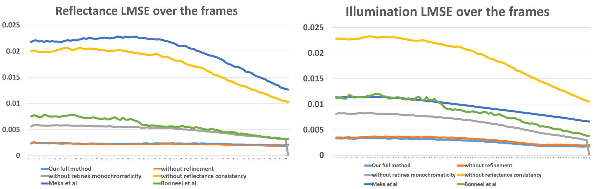
We perform quantitative evaluation on our SyntheticRoom sequence. The sequence was rendered using Blender’s Cycles renderer. All objects in the scene are assigned diffuse materials, with natural white illumination from the window. The objects in the scene cause significant inter-reflections. We also render the ground-truth reflectance and illumination images. We compare our decomposition to the ground-truth sequences and compute the LMSE error metric proposed by Grosse et al. 2009. We plot the LMSE error per-frame in Figure 5. We perform an ablation study by analyzing the error with our full energy and then removing some of the energy components, such as the base color refinement, the Retinex-monochromaticity prior and the spatiotemporal reflectance consistency prior. We also compare against state-of-the-art intrinsic video decomposition techniques. Our full method obtains the best results.


8.2. Qualitative Results
We show that the indirect illumination layers computed by our approach at real-time frame rates nicely capture the inter-reflections between various kinds of objects in a consistent manner, see Figures 1, 6, 7, 9 and 8. The brightness for all the indirect illumination layers shown in the paper has been scaled by for better visualization. In contrast to intrinsic decomposition approaches, ours separates the input image into reflectance, colored direct and indirect illumination layers. Please note the color bleeding of the different parts of the boat in Figure 1, which is clearly visible and nicely reconstructed, even though it only accounts for a small amount of the lighting in the input image.

Figure 8 shows the illumination decomposition for a complex scene with fast motion and a difficult color palette. Our clustering strategy fails to achieve a meaningful segmentation of the scene. Yet, we are able to produce a plausible decomposition of this challenging scene. In particular, we are able to capture the color spill from the girl’s shirt to her neck and the inter-reflections on the ground from the bush in the background.


| Sequence | Figures | Interactions |
| Box2 | 2 | |
| Box | 3, 12 | 3 |
| Cart | 22 | 1 |
| Cups | 20, 21 | 1 |
| Hands | 1 | |
| Toys | 2, 13 | 5 |
| Boat | 1 | 0 |
| ChitChat | 6, 14 | 0 |
| Cornell | 4, 16 | 0 |
| Droid | 9, 10, 15 | 0 |
| Girl | 0 | |
| Girl2 | 8 | 0 |
| Kermit | 19 | 0 |
| Paper | 17 | 0 |
| Umbrella | 7 | 0 |
| SyntheticRoom | 18 | 0 |
Figure 9 shows another example of the reconstructed illumination layers, where the color bleeding of the red and blue walls onto the floor is clearly visible. This sequence also shows that our decomposition is temporally coherent and that the illumination layers instantly adapt to changes in the scene. This can best be seen in the supplemental video. Such a decomposition into direct and indirect illumination is of paramount importance for illumination-consistent recoloring. We show an example of this for the same scene in Figure 10. Here, we first recolor the yellow duck to purple, which influences the color of the floor. In another example, we recolor the walls from blue to red, and vice versa, which also consistently changes the inter-reflections on the floor. Please note that our decomposition is computed at real-time frame rates, which enables the user to explore these effects interactively. In Table 1, we list the number of user-clicks that were performed for each sequence. Please note that most of the sequences did not require user interaction. Where necessary, we required only a small number of clicks, owing to our region-tracking strategy.
To evaluate our method on more general and more complex scenes, which consist of more than just a few prominent objects, we test our method on images from the Intrinsic Images in the Wild dataset (Bell et al. 2014). This dataset consists of room-sized indoor scenes. Even though such scenes generally do not exhibit particularly strong global lighting effects, our method is still able to pick up the prominent colors and visualize the global color spills that occur due to them, as shown in Figure 11. Such scenes are challenging for our method to handle, but video editing tasks such as recoloring can still benefit from our decomposition, even in such a challenging setting. We obtain a weighted human disagreement rate (WHDR) of 27.2%, which is better than the baselines and other video decomposition techniques such as Meka et al. 2016.


8.2.1. Evaluation of Misclustering Correction
We evaluate our novel sparsity-based misclustering correction in Figures 12 and 13. In the presence of strong inter-reflections, such as the green color spill in the shadow of the box in Figure 12, estimating the correct reflectance is highly challenging. The state-of-the-art intrinsic decomposition approaches of Meka et al. 2016 and Bonneel et al. 2014 struggle in this scenario, and often miscluster the inter-reflection into the reflectance map, see Figure 13. This causes severe problems when an inter-reflection-consistent recoloring of the scene is required, e.g. if the green wall should be virtually replaced by a blue wall. Our method alleviates this problem with a minimal amount of user interaction. With a single click, the misclustered region is identified, and our approach then automatically finds the correct reflectance based on our novel correction strategy that exploits the sparsity of the indirect illumination decomposition (see Section 5.2). Thus, the reflectance, direct and indirect illumination layers computed by our approach enable the seamless inter-reflection-consistent recoloring of scene elements, as shown in Figure 12.
8.2.2. Evaluation of the Sparsity Prior
We evaluate the importance of the sparsity prior in Figure 15 by comparing our illumination decomposition result with and without the illumination sparsity prior (Equation 11). Without the sparsity prior, the indirect illumination layers show activations across the entire image domain, which is inaccurate. Our sparsity prior forces inter-reflections to be explained by a small number of base colors; thus the optimization has to choose how to optimally explain the inter-reflections. This leads to sparser and more realistic indirect illumination layers that enable accurate inter-reflection-consistent recoloring. Note that with the sparsity prior – as expected from physical light transport – the contribution of the walls to the global illumination is limited to the regions close to the walls and in direct sight.
8.2.3. Evaluation of the Soft-Color-Retinex Weight
We evaluate the importance of the soft-color-Retinex weight in the illumination monochromaticity prior in Figure 14. Without the soft-Retinex weight, the prominent blue color spill on the wall and the red spill on the white shirt both incorrectly end up in the reflectance layer. This problem is easily resolved by the soft-Retinex weight.
8.3. Comparisons
We show a ground-truth comparison on synthetic data in Figure 16. In the following, we compare to the decomposition approaches of Carroll et al. 2011, Bonneel et al. 2014 and Meka et al. 2016.
8.3.1. Comparison to Carroll et al. 2011
While our illumination layer decomposition is inspired by Carroll et al. 2011, it builds on top of it in a significant way, as we list below:
- •
Carroll et al. 2011 assume that the intrinsic decomposition and base colors are given by Bousseau et al. 2009, whereas our method jointly performs intrinsic decomposition and base color estimation with the global illumination decomposition.
- •
Carroll et al. 2011 require the user to select the base colors that contribute to the indirect illumination in the scene, whereas our clustering-based strategy automatically identifies the base colors, which are then further refined jointly with the estimation of the indirect illumination layers.
- •
Carroll et al. 2011 use the sparsity of the indirect layers to accurately perform the illumination decomposition. We additionally use this sparsity property to enhance the quality of the reflectance estimation through the base color refinement and also to automate the misclustering correction.
- •
Both methods require the user to specify the regions in which the illumination decomposition is incorrect, but their method uses strokes whereas our method uses a single click for a region, and automatically identifies the correct underlying reflectance, which is propagated across the whole region/video.
- •
While both the methods use the IRLS strategy to solve the sparse and non-linear illumination decomposition problem, our method also optimizes for the reflectance layer and the base colors, which leads to an additional low-dimensional dense problem. We use a parallelized iterative solver to solve both problems jointly in real time. Combined with our region-tracking strategy, this enables our method to run on a live video and not just a single image.
We show a comparison in Figure 17. Their result retains too much color in the colored paper regions of the indirect illumination layers (Figure 17, bottom), resulting in a direct illumination layer that is not uniform across the table and the papers. Our base color refinement ensures that the illumination image retains only the global illumination (Figure 17, top), and that the color variation that stems from actual surface reflectance variation is moved to the reflectance layer. This causes our illumination layers to be more sparse, while accurately representing the color spill from the paper. Note that we obtain these results automatically, while Carroll et al. 2011’s approach requires several user scribbles. Unfortunately, further comparisons on other sequences cannot be shown due to unavailability of their code/implementation for this method.


8.3.2. Comparison to Bonneel et al. 2014 and Meka et al. 2016
We also compare against the intrinsic video decomposition techniques of Meka et al. 2016 and Bonneel et al. 2014. While these techniques make similar assumptions about the scene light transport as our method, they do not estimate the indirect illumination layers or the reflectance base colors. Our joint optimization leads to more accurate decomposition as we will show in a series of comparisons. While these two methods and our method all solve a high-dimensional non-linear optimization problem, our method also jointly solves the dense low-dimensional problem of base color refinement. Owing to the sparsity priors on the indirect illumination layers, this gives additional priors for the reflectance estimation.
In Figure 18, we analyze our base color refinement strategy on a synthetic sequence. Without the refinement, the illumination is inaccurately estimated to be blueish in multiple places, which is resolved by our refinement strategy. The other methods obtain globally inconsistent illumination results, and incorrectly bake the color spills into the reflectance layer. In Figure 19, we compare to the live intrinsic video decomposition approach of Meka et al. 2016. Their approach does not correctly handle inter-reflections, while our approach enables inter-reflection-consistent recoloring of scene objects. Please note the color bleeding from the green frog onto the hand. We show a second comparison in Figure 13, where we also compare to the off-line intrinsic video decomposition approach of Bonneel et al. 2014. Neither of these methods is able to correctly handle scene inter-reflections. Our supplemental videos contain additional comparisons to both methods.
8.4. Interactive Live Applications
We demonstrate several live video applications based on our illumination decomposition approach, such as inter-reflection-consistent recoloring and color keying. For a survey of digital keying methods we refer to Schultz and Hermes 2006.

8.4.1. Inter-Reflection-Consistent Recoloring
Our illumination decomposition approach enables inter-reflection-consistent recoloring of live video streams. We can recolor an object by modifying its associated base color, which also consistently recolors the object’s indirect illumination layer. To recolor the reflectance map, we employ our region-growing algorithm to identify the pixels belonging to a user-selected object based on their similarity to the object’s base color. We have already shown several plausible inter-reflection-consistent recoloring results in Figures 10, 12, 13 and 19, which outperform existing intrinsic image decomposition approaches (Meka et al. 2016; Bonneel et al. 2014). In Figure 20, we further demonstrate that our approach can even recolor subtle inter-reflections on glass, and not just on diffuse surfaces.
8.4.2. Inter-Reflection-Consistent Color Keying
Color keying is a technique often used in visual effects for overlaying a subject in a video on top of a different background using a color-based segmentation. In practice, a uniform green background is often used. Global light transport in the scene often causes green inter-reflections from the background onto the subject. This leads to unrealistic composites, since a green color spill is often visible on the subject, which does not match the new background. Our interactive illumination approach can be used to alleviate this problem, as shown in Figure 12. We first separate the input video into its direct and indirect illumination components. Afterwards, we modify the base color of the green indirect illumination layer, which relights the subject to better match the new background. This leads to more realistic outputs and can be achieved at interactive frame rates with our approach.

8.4.3. Color-Spill Suppression
In many video editing tasks, suppressing a strong color spill is highly important. This technique is often used in movie and television productions to suppress the spill from a green or blue-screen. We show an example of such an application in Figure 21. We are able to successfully suppress the spill from the shiny yellow cup by removing the indirect illumination layer of the cup from the illumination decomposition and recombining the other layers. We compare our results with state-of-the-art commercial software. The tested software is not able to suppress the spill for a particular object, but only for a particular color scheme. We also manually tuned the parameters of the software to achieve the best results. After optimizing the parameters, Adobe Premiere Pro CC is able to suppress the spill from the cup, but it also incorrectly modifies the color of the green cup on the left side. As is evident, our approach achieves the best results.
9. Discussion & Limitations

While we have demonstrated high-quality illumination decomposition results and a wide range of applications, our approach still has some limitations that we hope are addressed in follow-up work. Our method operates under a few assumptions, namely, diffuse materials, smooth camera motion, white direct illumination and consistent base colors throughout the video. Breaking these assumptions can lead to inaccurate estimations. For example, Figure 20 shows a scene with a specular yellow mug. Since the surface of the mug is not diffuse, our method incorrectly decomposes the specular highlight into the illumination layer. Nonetheless, we are still able to perform a realistic recoloring of the mug. In Figure 18, the illuminant in the scene is not white but has a yellowish hue. While you see that in the ground truth the yellow hue is present in the illumination layer, our decomposition incorrectly places it in the reflectance layer. This does not break down the method completely, but it can lead to slightly inaccurate results. Solving for the color of the illuminant in the scene would require additionally solving the ‘color-constancy’ problem, which makes the formulation even more ambiguous. This would be an interesting avenue for future work.
We also show in the Box2 sequence in the supplementary video (at 03:16) that our method can face challenges if objects enter or leave the scene during the course of the video. Modeling effects of objects that enter or leave the scene requires dynamically estimating and refining the base colors, which is computationally more challenging.
Our approach takes a monocular video as input and hence cannot model parts of the scene that are outside the view of the camera. This means that inter-reflections caused by out-of-view objects cannot be properly modeled, since the corresponding base color might not be available. This is a common limitation of all illumination decomposition approaches, including Carroll et al. 2011.
A further restriction is the user-specified upper bound on the number of base colors. If an object with an unseen color enters the scene for the first time, and the base colors are already exceeded, its inter-reflections cannot be modeled. This limitation could be alleviated in the future with a dynamic clustering strategy. Quick changes in camera view or abrupt scene motion can break our region propagation strategy. This could be alleviated by more sophisticated tracking strategies, such as SLAM.
Complex, textured scenes with many different colors are challenging to decompose, e.g. see Figure 22, since this requires many base colors, leading to a large number of variables and an even more under-constrained optimization problem. More sophisticated – potentially learned – scene priors could be beneficial. Our approach only obtains plausible decompositions, since we only model light transport up to the first bounce. Modeling the higher-order bounces would require a dramatic increase in the number of base colors, since all mixtures of reflectances would need to be considered.
More general indoor and outdoor scenes such as those in the Intrinsic Images in the Wild dataset (Bell et al. 2014) are not the ideal use cases for our method. This is because the scene illumination is often extremely complex, e.g., due to colored light sources and tinted windows. Like most approaches, ours assumes white direct illumination. Dealing with colored light sources is a more challenging problem due to the larger number of variables and thus greater ambiguity in the decomposition. Yet, assuming some level of sparsity in the color of the light sources, the problem could still be solved using a similar formulation as ours. We believe that this would be an interesting direction for future work.
Our decomposition results are generally temporally stable owing to the spatiotemporal reflectance consistency prior, but may exhibit some mild flickering effects at times, either due to the frequency of the indoor light sources or sudden changes in camera capture settings such as the camera aperture or auto focus or due to noise in the captured video. Flickering in some such sequences, such as the Box sequence has been discussed in the supplementary video.
10. Conclusion
We have proposed the first illumination decomposition approach for videos. At the core of our approach are multiple interlinked energies that enable the estimation of the direct and indirect illumination layers based on a small set of jointly estimated base colors. The resulting decomposition problem is formulated using sparse and dense sets of non-linear equations that are solved in real time using a novel alternating data-parallel optimization strategy that is implemented on the GPU. We have demonstrated decomposition results that qualitatively improve on existing state-of-the-art methods. In addition, we have demonstrated various compelling appearance editing applications. We hope that our approach will inspire follow-up work in this field.
Acknowledgements.
We thank the participants of the video sequences used in this work, particularly Jiayi Wang, Lingjie Liu and Edgar Tretschk. We also thank Carroll et al. [2012] and Bonneel et al. [2014] for providing their results in their supplementary material for comparisons. We also thank the authors of ‘Intrinsic Images in the Wild’ [Bell et al. 2014] for making their dataset available to the public. Abhimitra Meka and Christian Theobalt were supported by the ERC Consolidator Grant 4DRepLy (770784), Michael Zollhoefer was supported by Max Planck Center for Visual Computing and Communications (MPC-VCC) and Christian Richardt was supported by RCUK grant CAMERA (EP/M023281/1) and EPSRC-UKRI Innovation Fellowship (EP/S001050/1).References
- (1)
- Aksoy et al. (2016) Yağız Aksoy, Tunç Ozan Aydın, Marc Pollefeys, and Aljoša Smolić. 2016. Interactive high-quality green-screen keying via color unmixing. ACM Trans. Graph. 35, 5 (August 2016), 152:1–12. https://doi.org/10.1145/2907940
- Aksoy et al. (2017) Yağız Aksoy, Tunç Ozan Aydın, Aljoša Smolić, and Marc Pollefeys. 2017. Unmixing-Based Soft Color Segmentation for Image Manipulation. ACM Trans. Graph. 36, 2 (March 2017), 19:1–19. https://doi.org/10.1145/3002176
- Alperovich and Goldluecke (2017) Anna Alperovich and Bastian Goldluecke. 2017. A Variational Model for Intrinsic Light Field Decomposition. In ACCV. 66–82. https://doi.org/10.1007/978-3-319-54187-7_5
- Azinović et al. (2019) Dejan Azinović, Tzu-Mao Li, Anton Kaplanyan, and Matthias Nießner. 2019. Inverse Path Tracing for Joint Material and Lighting Estimation. In CVPR. 2442–2451. https://doi.org/10.1109/CVPR.2019.00255
- Bach et al. (2012) Francis Bach, Rodolphe Jenatton, Julien Mairal, and Guillaume Obozinski. 2012. Optimization with Sparsity-Inducing Penalties. Foundations and Trends in Machine Learning 4, 1 (2012), 1–106. https://doi.org/10.1561/2200000015
- Barron and Malik (2015) Jonathan T. Barron and Jitendra Malik. 2015. Shape, Illumination, and Reflectance from Shading. IEEE Trans. Pattern Anal. Mach. Intell. 37, 8 (August 2015), 1670–1687. https://doi.org/10.1109/TPAMI.2014.2377712
- Barrow and Tenenbaum (1978) Harry G. Barrow and Jay M. Tenenbaum. 1978. Recovering intrinsic scene characteristics from images. In Computer Vision Systems. 3–26.
- Beigpour and van de Weijer (2011) Shida Beigpour and Joost van de Weijer. 2011. Object recoloring based on intrinsic image estimation. In ICCV. 327–334. https://doi.org/10.1109/ICCV.2011.6126259
- Bell et al. (2014) Sean Bell, Kavita Bala, and Noah Snavely. 2014. Intrinsic Images in the Wild. ACM Trans. Graph. 33, 4 (July 2014), 159:1–12. https://doi.org/10.1145/2601097.2601206
- Bi et al. (2015) Sai Bi, Xiaoguang Han, and Yizhou Yu. 2015. An Image Transform for Edge-Preserving Smoothing and Scene-Level Intrinsic Decomposition. ACM Trans. Graph. 34, 4 (July 2015), 78:1–12. https://doi.org/10.1145/2766946
- Bi et al. (2018) Sai Bi, Nima Khademi Kalantari, and Ravi Ramamoorthi. 2018. Deep Hybrid Real and Synthetic Training for Intrinsic Decomposition. In Eurographics Symposium on Rendering – Experimental Ideas & Implementations.
- Bonneel et al. (2017) Nicolas Bonneel, Balazs Kovacs, Sylvain Paris, and Kavita Bala. 2017. Intrinsic Decompositions for Image Editing. Comput. Graph. Forum 36, 2 (May 2017), 593–609. https://doi.org/10.1111/cgf.13149
- Bonneel et al. (2014) Nicolas Bonneel, Kalyan Sunkavalli, James Tompkin, Deqing Sun, Sylvain Paris, and Hanspeter Pfister. 2014. Interactive Intrinsic Video Editing. ACM Trans. Graph. 33, 6 (November 2014), 197:1–10. https://doi.org/10.1145/2661229.2661253
- Bonneel et al. (2015) Nicolas Bonneel, James Tompkin, Kalyan Sunkavalli, Deqing Sun, Sylvain Paris, and Hanspeter Pfister. 2015. Blind Video Temporal Consistency. ACM Trans. Graph. 34, 6 (November 2015), 196:1–9. https://doi.org/10.1145/2816795.2818107
- Bousseau et al. (2009) Adrien Bousseau, Sylvain Paris, and Frédo Durand. 2009. User-Assisted Intrinsic Images. ACM Trans. Graph. 28, 5 (December 2009), 130:1–10. https://doi.org/10.1145/1618452.1618476
- Carroll et al. (2011) Robert Carroll, Ravi Ramamoorthi, and Maneesh Agrawala. 2011. Illumination decomposition for material recoloring with consistent interreflections. ACM Trans. Graph. 30, 4 (July 2011), 43:1–10. https://doi.org/10.1145/2010324.1964938
- Chang et al. (2014) Jason Chang, Randi Cabezas, and John W. Fisher, III. 2014. Bayesian Nonparametric Intrinsic Image Decomposition. In ECCV, Vol. 8692. 704–719. https://doi.org/10.1007/978-3-319-10593-2_46
- DeVito et al. (2017) Zachary DeVito, Michael Mara, Michael Zollhöfer, Gilbert Bernstein, Jonathan Ragan-Kelley, Christian Theobalt, Pat Hanrahan, Matthew Fisher, and Matthias Nießner. 2017. Opt: A Domain Specific Language for Non-Linear Least Squares Optimization in Graphics and Imaging. ACM Trans. Graph. 36, 5 (October 2017), 171:1–27. https://doi.org/10.1145/3132188
- Ding et al. (2017) Shouhong Ding, Bin Sheng, Xiaonan Hou, Zhifeng Xie, and Lizhuang Ma. 2017. Intrinsic Image Decomposition Using Multi-Scale Measurements and Sparsity. Comput. Graph. Forum 36, 6 (2017), 251–261. https://doi.org/10.1111/cgf.12874
- Dong et al. (2015) Bo Dong, Yue Dong, Xin Tong, and Pieter Peers. 2015. Measurement-based Editing of Diffuse Albedo with Consistent Interreflections. ACM Trans. Graph. 34, 4 (July 2015), 112:1–11. https://doi.org/10.1145/2766979
- Dong et al. (2014) Yue Dong, Guojun Chen, Pieter Peers, Jiawan Zhang, and Xin Tong. 2014. Appearance-from-motion: Recovering Spatially Varying Surface Reflectance Under Unknown Lighting. ACM Trans. Graph. 33, 6 (November 2014), 193:1–12. https://doi.org/10.1145/2661229.2661283
- Favreau et al. (2017) Jean-Dominique Favreau, Florent Lafarge, and Adrien Bousseau. 2017. Photo2ClipArt: Image Abstraction and Vectorization Using Layered Linear Gradients. ACM Trans. Graph. 36, 6 (November 2017), 180:1–11. https://doi.org/10.1145/3130800.3130888
- Garces et al. (2017) Elena Garces, Jose I. Echevarria, Wen Zhang, Hongzhi Wu, Kun Zhou, and Diego Gutierrez. 2017. Intrinsic Light Field Images. Comput. Graph. Forum 36, 8 (December 2017), 589–599. https://doi.org/10.1111/cgf.13154
- Garces et al. (2012) Elena Garces, Adolfo Muñoz, Jorge Lopez-Moreno, and Diego Gutierrez. 2012. Intrinsic Images by Clustering. Comput. Graph. Forum 31, 4 (2012), 1415–1424. https://doi.org/10.1111/j.1467-8659.2012.03137.x
- Georgoulis et al. (2018) Stamatios Georgoulis, Konstantinos Rematas, Tobias Ritschel, Efstratios Gavves, Mario Fritz, Luc Van Gool, and Tinne Tuytelaars. 2018. Reflectance and Natural Illumination from Single-Material Specular Objects Using Deep Learning. IEEE Trans. Pattern Anal. Mach. Intell. 40, 8 (August 2018), 1932–1947. https://doi.org/10.1109/TPAMI.2017.2742999
- Grosse et al. (2009) Roger Grosse, Micah K. Johnson, Edward H. Adelson, and William T. Freeman. 2009. Ground truth dataset and baseline evaluations for intrinsic image algorithms. In ICCV. 2335–2342. https://doi.org/10.1109/ICCV.2009.5459428
- Guo et al. (2017) Kaiwen Guo, Feng Xu, Tao Yu, Xiaoyang Liu, Qionghai Dai, and Yebin Liu. 2017. Real-time Geometry, Albedo and Motion Reconstruction Using a Single RGBD Camera. ACM Trans. Graph. 36, 3 (June 2017), 32:1–13. https://doi.org/10.1145/3083722
- Holland and Welsch (1977) Paul W. Holland and Roy E. Welsch. 1977. Robust regression using iteratively reweighted least-squares. Communications in Statistics – Theory and Methods 6, 9 (September 1977), 813–827. https://doi.org/10.1080/03610927708827533
- Innamorati et al. (2017) Carlo Innamorati, Tobias Ritschel, Tim Weyrich, and Niloy J. Mitra. 2017. Decomposing Single Images for Layered Photo Retouching. Comput. Graph. Forum 36, 4 (July 2017), 15–25. https://doi.org/10.1111/cgf.13220
- Janner et al. (2017) Michael Janner, Jiajun Wu, Tejas D. Kulkarni, Ilker Yildirim, and Joshua B. Tenenbaum. 2017. Self-Supervised Intrinsic Image Decomposition. In NIPS. http://rin.csail.mit.edu/
- Kajiya (1986) James T. Kajiya. 1986. The Rendering Equation. Computer Graphics (Proceedings of SIGGRAPH) 20, 4 (August 1986), 143–150. https://doi.org/10.1145/15886.15902
- Kim et al. (2016) Seungryong Kim, Kihong Park, Kwanghoon Sohn, and Stephen Lin. 2016. Unified Depth Prediction and Intrinsic Image Decomposition from a Single Image via Joint Convolutional Neural Fields. In ECCV. 143–159. https://doi.org/10.1007/978-3-319-46484-8_9
- Kong et al. (2014) Naejin Kong, Peter V. Gehler, and Michael J. Black. 2014. Intrinsic Video. In ECCV. 360–375. https://doi.org/10.1007/978-3-319-10605-2_24
- Kovacs et al. (2017) Balazs Kovacs, Sean Bell, Noah Snavely, and Kavita Bala. 2017. Shading Annotations in the Wild. In CVPR. 850–859. https://doi.org/10.1109/CVPR.2017.97
- Laffont et al. (2012) Pierre-Yves Laffont, Adrien Bousseau, Sylvain Paris, Frédo Durand, and George Drettakis. 2012. Coherent Intrinsic Images from Photo Collections. ACM Trans. Graph. 31, 6 (November 2012), 202:1–11. https://doi.org/10.1145/2366145.2366221
- Li et al. (2017) Xiao Li, Yue Dong, Pieter Peers, and Xin Tong. 2017. Modeling Surface Appearance from a Single Photograph Using Self-augmented Convolutional Neural Networks. ACM Trans. Graph. 36, 4 (July 2017), 45:1–11. https://doi.org/10.1145/3072959.3073641
- Li et al. (2018) Zhengqin Li, Zexiang Xu, Ravi Ramamoorthi, Kalyan Sunkavalli, and Manmohan Chandraker. 2018. Learning to Reconstruct Shape and Spatially-varying Reflectance from a Single Image. ACM Trans. Graph. 37, 6 (November 2018), 269:1–11. https://doi.org/10.1145/3272127.3275055
- Lin et al. (2017) Sharon Lin, Matthew Fisher, Angela Dai, and Pat Hanrahan. 2017. LayerBuilder: Layer Decomposition for Interactive Image and Video Color Editing. (2017). arXiv:1701.03754.
- Liu et al. (2017) Guilin Liu, Duygu Ceylan, Ersin Yumer, Jimei Yang, and Jyh-Ming Lien. 2017. Material Editing Using a Physically Based Rendering Network. In ICCV. 2280–2288. https://doi.org/10.1109/ICCV.2017.248
- Lombardi and Nishino (2016) Stephen Lombardi and Ko Nishino. 2016. Reflectance and Illumination Recovery in the Wild. IEEE Trans. Pattern Anal. Mach. Intell. 38, 1 (January 2016), 129–141. https://doi.org/10.1109/TPAMI.2015.2430318
- Marschner and Greenberg (1997) Stephen R. Marschner and Donald P. Greenberg. 1997. Inverse lighting for photography. In Proceedings of the IS&T Color Imaging Conference. 262–265.
- Meka et al. (2016) Abhimitra Meka, Michael Zollhöfer, Christian Richardt, and Christian Theobalt. 2016. Live Intrinsic Video. ACM Trans. Graph. 35, 4 (July 2016), 109:1–14. https://doi.org/10.1145/2897824.2925907
- Nam et al. (2018) Giljoo Nam, Joo Ho Lee, Diego Gutierrez, and Min H. Kim. 2018. Practical SVBRDF Acquisition of 3D Objects with Unstructured Flash Photography. ACM Trans. Graph. 37, 6 (November 2018), 267:1–12. https://doi.org/10.1145/3272127.3275017
- Narihira et al. (2015) Takuya Narihira, Michael Maire, and Stella X. Yu. 2015. Direct Intrinsics: Learning Albedo-Shading Decomposition by Convolutional Regression. In ICCV. https://doi.org/10.1109/ICCV.2015.342
- Nayar et al. (2006) Shree K. Nayar, Gurunandan Krishnan, Michael D. Grossberg, and Ramesh Raskar. 2006. Fast separation of direct and global components of a scene using high frequency illumination. ACM Trans. Graph. 25, 3 (July 2006), 935–944. https://doi.org/10.1145/1141911.1141977
- Nestmeyer and Gehler (2017) Thomas Nestmeyer and Peter V. Gehler. 2017. Reflectance Adaptive Filtering Improves Intrinsic Image Estimation. In CVPR. 1771–1780. https://doi.org/10.1109/CVPR.2017.192
- O’Toole et al. (2016) Matthew O’Toole, John Mather, and Kiriakos N. Kutulakos. 2016. 3D Shape and Indirect Appearance by Structured Light Transport. IEEE Trans. Pattern Anal. Mach. Intell. 38, 7 (July 2016), 1298–1312. https://doi.org/10.1109/TPAMI.2016.2545662
- Patow and Pueyo (2003) Gustavo Patow and Xavier Pueyo. 2003. A Survey of Inverse Rendering Problems. Comput. Graph. Forum 22, 4 (2003), 663–687. https://doi.org/10.1111/j.1467-8659.2003.00716.x
- Ramamoorthi and Hanrahan (2001) Ravi Ramamoorthi and Pat Hanrahan. 2001. A signal-processing framework for inverse rendering. In SIGGRAPH. 117–128. https://doi.org/10.1145/383259.383271
- Ren et al. (2015) Peiran Ren, Yue Dong, Stephen Lin, Xin Tong, and Baining Guo. 2015. Image Based Relighting Using Neural Networks. ACM Trans. Graph. 34, 4 (July 2015), 111:1–12. https://doi.org/10.1145/2766899
- Richardt et al. (2014) Christian Richardt, Jorge Lopez-Moreno, Adrien Bousseau, Maneesh Agrawala, and George Drettakis. 2014. Vectorising Bitmaps into Semi-Transparent Gradient Layers. Comput. Graph. Forum 33, 4 (June 2014), 11–19. https://doi.org/10.1111/cgf.12408
- Schultz and Hermes (2006) Christopher Schultz and Thorsten Hermes. 2006. Digital Keying Methods. TZI-Bericht 40. Technologie-Zentrum Informatik, Bremen University. http://www.tzi.de/fileadmin/resources/publikationen/tzi_berichte/TZI-Bericht-Nr._40.pdf
- Seitz et al. (2005) Steven M. Seitz, Yasuyuki Matsushita, and Kiriakos N. Kutulakos. 2005. A theory of inverse light transport. In ICCV, Vol. 2. 1440–1447. https://doi.org/10.1109/ICCV.2005.25
- Shen et al. (2014) Jianbing Shen, Xing Yan, Lin Chen, Hanqiu Sun, and Xuelong Li. 2014. Re-texturing by intrinsic video. Information Sciences 281 (October 2014), 726–735. https://doi.org/10.1016/j.ins.2014.02.134
- Shen et al. (2011) Jianbing Shen, Xiaoshan Yang, Yunde Jia, and Xuelong Li. 2011. Intrinsic images using optimization. In CVPR. 3481–3487. https://doi.org/10.1109/CVPR.2011.5995507
- Shi et al. (2017) Jian Shi, Yue Dong, Hao Su, and Stella X. Yu. 2017. Learning Non-Lambertian Object Intrinsics across ShapeNet Categories. In CVPR. 5844–5853. https://doi.org/10.1109/CVPR.2017.619
- Tan et al. (2018) Jianchao Tan, Jose Echevarria, and Yotam Gingold. 2018. Efficient Palette-based Decomposition and Recoloring of Images via RGBXY-space Geometry. ACM Trans. Graph. 37, 6 (November 2018), 262:1–10. https://doi.org/10.1145/3272127.3275054
- Tan et al. (2016) Jianchao Tan, Jyh-Ming Lien, and Yotam Gingold. 2016. Decomposing Images into Layers via RGB-space Geometry. ACM Trans. Graph. 36, 1 (November 2016), 7:1–14. https://doi.org/10.1145/2988229
- Wu et al. (2014) Chenglei Wu, Michael Zollhöfer, Matthias Nießner, Marc Stamminger, Shahram Izadi, and Christian Theobalt. 2014. Real-time Shading-based Refinement for Consumer Depth Cameras. ACM Trans. Graph. 33, 6 (November 2014), 200:1–10. https://doi.org/10.1145/2661229.2661232
- Wu et al. (2016) Hongzhi Wu, Zhaotian Wang, and Kun Zhou. 2016. Simultaneous Localization and Appearance Estimation with a Consumer RGB-D Camera. IEEE Trans. Vis. Comput. Graph. 22, 8 (August 2016), 2012–2023. https://doi.org/10.1109/TVCG.2015.2498617
- Ye et al. (2014) Genzhi Ye, Elena Garces, Yebin Liu, Qionghai Dai, and Diego Gutierrez. 2014. Intrinsic Video and Applications. ACM Trans. Graph. 33, 4 (July 2014), 80:1–11. https://doi.org/10.1145/2601097.2601135
- Yu et al. (1999) Yizhou Yu, Paul Debevec, Jitendra Malik, and Tim Hawkins. 1999. Inverse global illumination: recovering reflectance models of real scenes from photographs. In SIGGRAPH. 215–224. https://doi.org/10.1145/311535.311559
- Zhou et al. (2015) Tinghui Zhou, Philipp Krähenbühl, and Alyosha Efros. 2015. Learning Data-driven Reflectance Priors for Intrinsic Image Decomposition. In ICCV. 3469–3477. https://doi.org/10.1109/ICCV.2015.396
- Zollhöfer et al. (2014) Michael Zollhöfer, Matthias Nießner, Shahram Izadi, Christoph Rhemann, Christopher Zach, Matthew Fisher, Chenglei Wu, Andrew Fitzgibbon, Charles Loop, Christian Theobalt, and Marc Stamminger. 2014. Real-time Non-rigid Reconstruction Using an RGB-D Camera. ACM Trans. Graph. 33, 4 (July 2014), 156:1–12. https://doi.org/10.1145/2601097.2601165
- Zoran et al. (2015) Daniel Zoran, Phillip Isola, Dilip Krishnan, and William T. Freeman. 2015. Learning Ordinal Relationships for Mid-Level Vision. In ICCV. 388–396. https://doi.org/10.1109/ICCV.2015.52