跳到论文正文
W Papers独立论文阅读器 arXiv:1908.01892 论文正文 计算阅读时间 · 0%
引用这篇论文根据当前论文元数据生成,正式投稿前建议核对。


License: arXiv.org perpetual non-exclusive license
arXiv:1908.01892v1 [math.NA] 05 Aug 2019

A new unified stabilized mixed finite element method of the Stokes-Darcy coupled problem: Isotropic discretization

Houédanou Koffi Wilfrid (a) Email address: a) khouedanou@yahoo.fr Address: Département de Mathématiques, Université d’Abomey-Calavi (UAC), Rep. of Benin
Abstract.

In this paper we develop an a priori error analysis of a new unified mixed finite element method for the coupling of fluid flow with porous media flow in ℝN\mathbb{R}^{N}, N∈{2,3}N\in\{2,3\} on isotropic meshes. Flows are governed by the Stokes and Darcy equations, respectively, and the corresponding transmission conditions are given by mass conservation, balance of normal forces, and the Beavers-Joseph-Saffman law. The approach utilizes a modification of the Darcy problem which allows us to apply a variant nonconforming Crouzeix-Raviart finite element to the whole coupled Stokes-Darcy problem. The well-posedness of the finite element scheme and its convergence analysis are derived. Finally, the numerical experiments are presented, which confirm the excellent stability and accuracy of our method.
Keywords : Coupled Stokes and Darcy flows; Nonconforming finite element method; Crouzeix-Raviart element.
Mathematics Subject Classification [MSC]: 74S05, 74S10, 74S15, 74S20, 74S25, 7430.

1. Introduction

There are many serious problems currently facing the world in which the coupling between groundwater and surface water is important. These include questions such as predicting how pollution discharges into streams, lakes, and rivers making its way into the water supply. This coupling is also important in technological applications involving filtration. We refer to the nice overview [9] and the references therein for its physical background, modeling, and standard numerical methods. One important issue in the modeling of the coupled Darcy-Stokes flow is the treatement of the interface condition, where the Stokes fluid meets the porous medium. In this paper, we only consider the so-called Beavers-Joseph-Saffman condition, which was experimentally derived by Beavers and Joseph in [4], modified by Saffman in [31], and later mathematically justified in [20, 21, 23, 28].

It is well known that the discretization of the velocity and the pressure, for both Stokes and Darcy problems and the coupled of them, has to be made in a compatible way in order to avoid instabilities. Since, usually, stable elements for the free fluid flow cannot been successfully applied to the porous medium flow, most of the finite element formulations developed for the Stokes-Darcy coupled problem are based on appropriate combinations of stable elements for the Stokes equations with stable elements for the Darcy equations. In [19, 32, 27, 33, 25, 26, 30, 1, 12, 15, 20, 23, 22, 29, 6, 3, 13, 2, 34, 24, 18], and in the references therein, we can find a large list of contributions devoted to numerically approximate the solution of this interaction problem, including conforming and nonconforming methods.

There are a lot of papers considering different finite element spaces in each flow region (see, for example, [14, 8, 13] and the references therein). In contrast to this, other articles use the same finite element spaces in both regions by, in general, introducing some penalizing terms (ref. for examples [2, 30, 27] and the references therein).

In [2], a conforming unified finite element has been proposed for the modified coupled Stokes-Darcy problem in a plane domain, which has simple and straightforward implementations. The authors apply the classical Mini-element to the whole coupled Stokes-Darcy coupled problem. An a priori error analysis is performed with some numerical tests confirming the convergence rates.

In this article, we propose a modification of the Darcy problem which allows us to apply a variant nonconforming finite element to the whole coupled Stokes-Darcy problem. We use a variant nonconforming Crouzeix-Raviart finite element method that has so many advantages for the velocities and piecewise constant for the pressures in both the Stokes and Darcy regions, and apply a stabilization term penalizing the jumps over the element edges of the piecewise continuous velocities. We prove that the formulation satisfies the discrete inf-sup conditions, obtaining as a result optimal accuracy with respect to solution regularity. Numerical experimants are also presented, which confirm the excellent stability and optimal performance of our method. The difference between our paper and the reference [2] is that our discretization is nonconforming in both the Stokes domain and Darcy domain (in Ω⊂ℝN\Omega\subset\mathbb{R}^{N}, N=2​ or ​3N=2\mbox{ or }3). As a result, additional terms are included in the priori error analysis that measure the non-conformity of the method. One essential difficulty in choosing the unified discretization is that, the Stokes side velocity is in H1H^{1} while the Darcy side velocity is only in H⁡(div)H(\mathop{\rm div}\nolimits). Thus, we introduce a variant of the nonconforming Crouzeix-Raviart piecewise linear finite element space (larger than the space Hh\textbf{H}_{h} used in [30]). The choice of Hh\textbf{H}_{h} [see (38)] is more natural than the one introduced in [30] since the space Hh\textbf{H}_{h} approximates only H(div,Ωd)H(\mathop{\rm div}\nolimits,\Omega_{d}) and not [H1​(Ωd)]N[H^{1}(\Omega_{d})]^{N}, while our a priori error analysis is only valid in this larger space.

The rest of the paper is organized as follows. In Section 2 we present the modified coupled Stokes-Darcy problem in Ω⊂ℝN\Omega\subset\mathbb{R}^{N}, N=2​ or ​3N=2\mbox{ or }3, notations and the weak formulation. Section 3 is devoted to the finite element discretization and the error estimation. Finally, in Section 4, we present the results of numerical experiments to verify the predicted rates of convergence.

2. Preliminaries and notation

2.1. Model problem

We consider the model of a flow in a bounded domain Ω⊂ℝN\Omega\subset\mathbb{R}^{N} (N=2​ or ​3)(N=2\mbox{ or }3), consisting of a porous medium domain Ωd\Omega_{d}, where the flow is a Darcy flow, and an open region Ωs=Ω∖Ω¯d,\Omega_{s}=\Omega\smallsetminus\overline{\Omega}_{d}, where the flow is governed by the Stokes equations. The two regions are separated by an interface ΓI=∂Ωd∩∂Ωs.\Gamma_{I}=\partial\Omega_{d}\cap\partial\Omega_{s}. Let Γl=∂Ωl∖ΓI\Gamma_{l}=\partial\Omega_{l}\smallsetminus\Gamma_{I}, l=s,dl=s,d. Each interface and boundary is assumed to be polygonal (N=2)(N=2) or polyhedral (N=3)(N=3). We denote by ns\textbf{n}_{s} (resp. nd\textbf{n}_{d}) the unit outward normal vector along ∂Ωs\partial\Omega_{s} (resp. ∂Ωd\partial\Omega_{d}). Note that on the interface ΓI\Gamma_{I}, we have ns=−nd\textbf{n}_{s}=-\textbf{n}_{d}. The Figures 2 and 2 give a schematic representation of the geometry.

Ωd\Omega_{d}: Porous Medium Ωs\Omega_{s}: Fluid Region nd\textbf{n}_{d}ns\textbf{n}_{s}τj\tau_{j}ΓI\Gamma_{I}Γd\Gamma_{d}Γd\Gamma_{d}Γd\Gamma_{d}Γs\Gamma_{s}Γs\Gamma_{s}Γs\Gamma_{s}
Figure 1. A sketch of the geometry of the problem (case: ∂Ωd≠ΓI\partial\Omega_{d}\neq\Gamma_{I})
Γs\Gamma_{s}Γd\Gamma_{d} Ωs\Omega_{s}: Fluid Region Ωd:Porous Medium\Omega_{d}:\mbox{{\small\small\small Porous Medium}}ns\textbf{n}_{s}τj\tau_{j}
Figure 2. A sketch of the geometry of the problem (case ∂Ωd=ΓI.\partial\Omega_{d}=\Gamma_{I}.)

For any function vv defined in Ω\Omega, since its restriction to Ωs\Omega_{s} or to Ωd\Omega_{d} could play a different mathematical roles (for instance their traces on ΓI\Gamma_{I}), we will set vs=v|Ωsv_{s}=v_{|\Omega_{s}} and vd=v|Ωdv_{d}=v_{|\Omega_{d}}.

In Ω\Omega, we denote by u the fluid velocity and by pp the pressure. The motion of the fluid in Ωs\Omega_{s} is described by the Stokes equations

{−2μdivD(u)+∇p=f in Ωs,divu=g in Ωs,u=0 on Γs,\displaystyle\left\{\begin{array}[]{ccccccccc}-2\mu\mathop{\rm div}\nolimits\textbf{D}(\textbf{u})+\nabla p&=&\textbf{f}&\mbox{ in }&&\Omega_{s},&\\ \mathop{\rm div}\nolimits\textbf{u}&=&g&\mbox{ in }&&\Omega_{s},&\\ \textbf{u}&=&\textbf{0}&\mbox{ on }&&\Gamma_{s},&\end{array}\right.

while in the porous medium Ωd\Omega_{d}, by Darcy’s law

{μ​K−1​𝐮+∇p=f in Ωd,divu=g in Ωd,u⋅nd=0 on Γd.\displaystyle\left\{\begin{array}[]{cccccccccccc}\mu\textbf{K}^{-1}\mathbf{u}+\nabla p&=&\textbf{f}&\mbox{ in }&&\Omega_{d},&\\ \mathop{\rm div}\nolimits\textbf{u}&=&g&\mbox{ in }&&\Omega_{d},&\\ \textbf{u}\cdot\textbf{n}_{d}&=&0&\mbox{ on }&&\Gamma_{d}.&\end{array}\right.

Here, μ>0\mu>0 is the fluid viscosity, D the deformation rate tensor defined by

D(ψ)i​j:=12(∂ψi∂xj+∂ψj∂xi), 1⩽i,j⩽N,\displaystyle\textbf{D}(\psi)_{ij}:=\frac{1}{2}\left(\frac{\partial\psi_{i}}{\partial x_{j}}+\frac{\partial\psi_{j}}{\partial x_{i}}\right),\mbox{ }1\leqslant i,j\leqslant N,

and K a symmetric and uniformly positive definite tensor representing the rock permeability and satisfying, for some constants 0<K∗⩽K∗<+∞0<K_{*}\leqslant K^{*}<+\infty,

K∗ξTξ⩽ξTK(x)ξ⩽K∗ξTξ, ∀x∈Ωd, ξ∈ℝN.K_{*}\xi^{T}\xi\leqslant\xi^{T}\textbf{K}(x)\xi\leqslant K^{*}\xi^{T}\xi,\mbox{ }\forall x\in\Omega_{d},\mbox{ }\xi\in\mathbb{R}^{N}.

f∈[L2​(Ω)]N\textbf{f}\in[L^{2}(\Omega)]^{N} is a term related to body forces and g∈L2​(Ω)g\in L^{2}(\Omega) a source or sink term satisfying the compatibility condition

∫Ωg⁡(x)​𝑑x=0.\displaystyle\int_{\Omega}g(x)dx=0.

Finally we consider the following interface conditions on ΓI:\Gamma_{I}:

(9) us⋅ns+𝐮d⋅nd\displaystyle\textbf{u}_{s}\cdot\textbf{n}_{s}+\mathbf{u}_{d}\cdot\textbf{n}_{d} =\displaystyle= 0,\displaystyle 0,
(10) ps−2​μ​ns⋅D​(us)⋅ns\displaystyle p_{s}-2\mu\textbf{n}_{s}\cdot\textbf{D}(\textbf{u}_{s})\cdot\textbf{n}_{s} =\displaystyle= pd,\displaystyle p_{d},
(11) κjα1​2​ns⋅D​(us)⋅τj\displaystyle\frac{\sqrt{\kappa_{j}}}{\alpha_{1}}2\textbf{n}_{s}\cdot\textbf{D}(\textbf{u}_{s})\cdot\tau_{j} =\displaystyle= −us⋅τj, j=1,…,N−1.\displaystyle-\textbf{u}_{s}\cdot\tau_{j},\mbox{ }j=1,\ldots,N-1.

Here, Eq. (9) represents mass conservation, Eq. (10) the balance of normal forces, and Eq. (11) the Beavers-Joseph-Saffman conditions. Moreover, {τj}j=1,…,N−1\{\tau_{j}\}_{j=1,\ldots,N-1} denotes an orthonormal system of tangent vectors on ΓI\Gamma_{I}, κj=τj⋅K⋅τj\kappa_{j}=\tau_{j}\cdot\textbf{K}\cdot\tau_{j}, and α1\alpha_{1} is a parameter determined by experimental evidence.

Eqs. (2.1) to (11) consist of the model of the coupled Stokes and Darcy flows problem that we will study below.

2.2. New weak formulation

We begin this subsection by introducing some useful notations. If WW is a bounded domain of ℝN\mathbb{R}^{N} and mm is a non negative integer, the Sobolev space Hm​(W)=Wm,2​(W)H^{m}(W)=W^{m,2}(W) is defined in the usual way with the usual norm ∥⋅∥m,W\parallel\cdot\parallel_{m,W} and semi-norm |⋅|m,W|\cdot|_{m,W}. In particular, H0​(W)=L2​(W)H^{0}(W)=L^{2}(W) and we write ∥⋅∥W\parallel\cdot\parallel_{W} for ∥⋅∥0,W\parallel\cdot\parallel_{0,W}. Similarly we denote by (⋅,⋅)W(\cdot,\cdot)_{W} the L2​(W)L^{2}(W) [L2​(W)]N[L^{2}(W)]^{N} or [L2​(W)]N×N[L^{2}(W)]^{N\times N} inner product. For shortness if WW is equal to Ω\Omega, we will drop the index Ω\Omega, while for any m≥0m\geq 0, ∥⋅∥m,l=∥⋅∥m,Ωl\parallel\cdot\parallel_{m,l}=\parallel\cdot\parallel_{m,\Omega_{l}}, |⋅|m,l=|⋅|m,Ωl|\cdot|_{m,l}=|\cdot|_{m,\Omega_{l}} and (.,.)l=(⋅,⋅)Ωl(.,.)_{l}=(\cdot,\cdot)_{\Omega_{l}}, for l=s,dl=s,d. The space H0m​(Ω)H_{0}^{m}(\Omega) denotes the closure of C0∞​(Ω)C_{0}^{\infty}(\Omega) in Hm​(Ω)H^{m}(\Omega). Let [Hm​(Ω)]N[H^{m}(\Omega)]^{N} be the space of vector valued functions v=(v1,…,vN)\textbf{v}=(v_{1},\ldots,v_{N}) with components viv_{i} in Hm​(Ω)H^{m}(\Omega). The norm and the seminorm on [Hm​(Ω)]N[H^{m}(\Omega)]^{N} are given by

(12) ∥v∥m,Ω:=(∑i=0N∥vi∥m,Ω2)1/2 and |v|m,Ω:=(∑i=0N|vi|m,Ω2)1/2.\displaystyle\parallel\textbf{v}\parallel_{m,\Omega}\hskip 5.69046pt:=\hskip 5.69046pt\left(\sum_{i=0}^{N}\parallel v_{i}\parallel_{m,\Omega}^{2}\right)^{1/2}\mbox{ and }\hskip 5.69046pt|\textbf{v}|_{m,\Omega}\hskip 5.69046pt:=\hskip 5.69046pt\left(\sum_{i=0}^{N}|v_{i}|_{m,\Omega}^{2}\right)^{1/2}.

For a connected open subset of the boundary Γ⊂∂Ωs∪∂Ωd\Gamma\subset\partial\Omega_{s}\cup\partial\Omega_{d}, we write ⟨.,.⟩Γ\langle.,.\rangle_{\Gamma} for the L2​(Γ)L^{2}(\Gamma) inner product (or duality pairing), that is, for scalar valued functions λ\lambda, η\eta one defines:

(13) ⟨λ,η⟩Γ\displaystyle\langle\lambda,\eta\rangle_{\Gamma} :⁣=\displaystyle:= ∫Γλ⁡(s)⋅η⁡(s)​𝑑s\displaystyle\int_{\Gamma}\lambda(s)\cdot\eta(s)ds

We also define the special vector-valued functions space

(14) H(div,Ω)\displaystyle\textbf{H}(\mathop{\rm div}\nolimits,\Omega) :⁣=\displaystyle:= {v∈[L2​(Ω)]N:divv∈L2​(Ω)}\displaystyle\left\{\textbf{v}\in[L^{2}(\Omega)]^{N}:\mathop{\rm div}\nolimits\textbf{v}\in L^{2}(\Omega)\right\}

To give the variational formulation of our coupled problem we define the following two spaces for the velocity and the pressure:

H :⁣=\displaystyle:= {v∈H(div,Ω):vs∈[H1(Ωs)]N, v=0 on Γs and v⋅nd=0 on Γd}\displaystyle\left\{\textbf{v}\in\textbf{H}(\mathop{\rm div}\nolimits,\Omega):\textbf{v}_{s}\in[H^{1}(\Omega_{s})]^{N},\textbf{ }\textbf{v}=\textbf{0}\mbox{ on }\Gamma_{s}\mbox{ and }\textbf{v}\cdot\textbf{n}_{d}=0\mbox{ on }\Gamma_{d}\right\}

equipped with the norm

(15) ∥v∥H\displaystyle\parallel\textbf{v}\parallel_{\textbf{H}} :⁣=\displaystyle:= (|v|1,s2+∥v∥d2+∥divv∥d2)1/2,\displaystyle\left(|\textbf{v}|_{1,s}^{2}+\parallel\textbf{v}\parallel_{d}^{2}+\parallel\mathop{\rm div}\nolimits\textbf{v}\parallel_{d}^{2}\right)^{1/2},

and

(16) Q=L02​(Ω):={q∈L2​(Ω):∫Ωq⁡(x)​𝑑x=0}.\displaystyle Q=L_{0}^{2}(\Omega):=\left\{q\in L^{2}(\Omega):\int_{\Omega}q(x)dx=0\right\}.

Multiplying the first equation of (2.1) by a test fonction 𝐯∈𝐇\bf v\in\bf H and the second one by q∈Qq\in Q, integrating by parts over Ωs\Omega_{s} the terms involving divD​(u)\mathop{\rm div}\nolimits\textbf{D}(\textbf{u}) and ∇p\nabla p, yield the variational form of Stokes equations:

(17) (fs,vs)Ωs\displaystyle(\textbf{f}_{s},\textbf{v}_{s})_{\Omega_{s}} =\displaystyle= 2​μ​(D​(us),D​(vs))Ωs−(ps,div vs)Ωs\displaystyle 2\mu\left(\textbf{D}(\textbf{u}_{s}),\textbf{D}(\textbf{v}_{s})\right)_{\Omega_{s}}-\left(p_{s},\mbox{div}\mbox{ }\textbf{v}_{s}\right)_{\Omega_{s}}
+\displaystyle+ ({ps−2​μ​ns⋅D​(us)⋅ns},vs⋅ns)ΓI\displaystyle\left(\left\{p_{s}-2\mu\textbf{n}_{s}\cdot\textbf{D}(\textbf{u}_{s})\cdot\textbf{n}_{s}\right\},\textbf{v}_{s}\cdot\textbf{n}_{s}\right)_{\Gamma_{I}}
+\displaystyle+ ∑j=1N−1(−2μns⋅D(us)⋅τj,vs⋅τj)ΓI\displaystyle\displaystyle\sum_{j=1}^{N-1}\left(-2\mu\textbf{n}_{s}\cdot\textbf{D}(\textbf{u}_{s})\cdot\tau_{j},\textbf{v}_{s}\cdot\tau_{j}\right)_{\Gamma_{I}}
(18) −(qs,div us)Ωs\displaystyle-\left(q_{s},\mbox{div}\mbox{ }\textbf{u}_{s}\right)_{\Omega_{s}} =\displaystyle= −(gs,qs)Ωs\displaystyle-(g_{s},q_{s})_{\Omega_{s}}

Using interface conditions (10)(\ref{cd2}) and (11)(\ref{cd3}) in (17), we obtain:

(19) (fs,v)Ωs\displaystyle(\textbf{f}_{s},\textbf{v})_{\Omega_{s}} =\displaystyle= 2​μ​(D​(us),D​(v))Ωs−(ps,div v)Ωs\displaystyle 2\mu\left(\textbf{D}(\textbf{u}_{s}),\textbf{D}(\textbf{v})\right)_{\Omega_{s}}-\left(p_{s},\mbox{div}\mbox{ }\textbf{v}\right)_{\Omega_{s}}
+\displaystyle+ (pd,vs⋅ns)ΓI+∑j=1N−1μ​α1kj(us⋅τj,vs⋅τj)ΓI ∀v∈H\displaystyle(p_{d},\textbf{v}_{s}\cdot\textbf{n}_{s})_{\Gamma_{I}}+\displaystyle\sum_{j=1}^{N-1}\frac{\mu\alpha_{1}}{\sqrt{k_{j}}}(\textbf{u}_{s}\cdot\tau_{j},\textbf{v}_{s}\cdot\tau_{j})_{\Gamma_{I}}\mbox{ }\forall\textbf{v}\in\textbf{H}
(20) −(q,div us)Ωs\displaystyle-\left(q,\mbox{div}\mbox{ }\textbf{u}_{s}\right)_{\Omega_{s}} =\displaystyle= −(gs,q)Ωs ∀q∈Q\displaystyle-(g_{s},q)_{\Omega_{s}}\mbox{ }\forall q\in Q

We apply a similar treatment to the Darcy equations by testing the first equation of (2.1) with a smooth fonction v∈H\textbf{v}\in\textbf{H} and the second on by q∈Qq\in Q, integrating by parts over Ωd\Omega_{d} the terms involving ∇pd\nabla p_{d}, yield the variational form of Darcy equations:

(21) (μ​K−1​ud,v)Ωd\displaystyle\left(\mu\textbf{K}^{-1}\textbf{u}_{d},\textbf{v}\right)_{\Omega_{d}} =\displaystyle= (pd,div v)Ωd+(fd,v)Ωd−(pd,vd⋅nd)ΓI ∀v∈H\displaystyle\left(p_{d},\mbox{div}\mbox{ }\textbf{v}\right)_{\Omega_{d}}+(\textbf{f}_{d},\textbf{v})_{\Omega_{d}}-(p_{d},\textbf{v}_{d}\cdot\textbf{n}_{d})_{\Gamma_{I}}\mbox{ }\forall\textbf{v}\in\textbf{H}
(22) (div ud,q)Ωd\displaystyle\left(\mbox{div}\mbox{ }\textbf{u}_{d},q\right)_{\Omega_{d}} =\displaystyle= (gd,q)Ωd ∀q∈Q\displaystyle\left(g_{d},q\right)_{\Omega_{d}}\mbox{ }\forall q\in Q

Now, incorporating the first boundary interface condition (9) and taking into account that the vector valued functions in H have (weakly) continuous normal components on ΓI\Gamma_{I} (see [16, Theorem 2.5]), the mixed variational formulation of the coupled problem (2.1)-(11) can be stated as follows [27]: Find (u,p)∈H×Q(\textbf{u},p)\in\textbf{H}\times Q that satisfies

(23) {a​(u,v)+b​(v,p)=L⁡(v),∀v∈H,b​(u,q)=G⁡(q),∀q∈Q.\left\{\begin{array}[]{ccc}\textbf{a}(\textbf{u},\textbf{v})+\textbf{b}(\textbf{v},p)&=&L(\textbf{v}),\hskip 28.45274pt\forall\textbf{v}\in\textbf{H},\\ \textbf{b}(\textbf{u},q)&=&G(q),\hskip 28.45274pt\forall q\in Q.\end{array}\right.

where the bilinear forms a​(⋅,⋅)\textbf{a}(\cdot,\cdot) and b​(⋅,⋅)\textbf{b}(\cdot,\cdot) are defined on H×H\textbf{H}\times\textbf{H} and H×Q\textbf{H}\times Q, respectively, as:

a​(u,v)\displaystyle\textbf{a}(\textbf{u},\textbf{v}) :⁣=\displaystyle:= 2​μ​(D​(u),D​(v))s+∑j=1N−1μ​α1κj​⟨us⋅τj,vs⋅τj⟩ΓI+μ​(K−1​u,v)d\displaystyle 2\mu(\textbf{D}(\textbf{u}),\textbf{D}(\textbf{v}))_{s}+\sum_{j=1}^{N-1}\frac{\mu\alpha_{1}}{\sqrt{\kappa_{j}}}\left\langle\textbf{u}_{s}\cdot\tau_{j},\textbf{v}_{s}\cdot\tau_{j}\right\rangle_{\Gamma_{I}}+\mu\left(\textbf{K}^{-1}\textbf{u},\textbf{v}\right)_{d}
b​(v,q)\displaystyle\textbf{b}(\textbf{v},q) :⁣=\displaystyle:= −(q,divv)Ωs−(q,divv)Ωd\displaystyle-\left(q,\mathop{\rm div}\nolimits\textbf{v}\right)_{\Omega_{s}}-\left(q,\mathop{\rm div}\nolimits\textbf{v}\right)_{\Omega_{d}}

By last, the linear forms LL and GG are defined as:

L⁡(v):=(f,v)Ωs+(f,v)Ωd and G⁡(q):=−(g,q)Ωs−(g,q)Ωd.\displaystyle L(\textbf{v}):=(\textbf{f},\textbf{v})_{\Omega_{s}}+(\textbf{f},\textbf{v})_{\Omega_{d}}\hskip 56.9055pt\mbox{ and }\hskip 56.9055ptG(q):=-(g,q)_{\Omega_{s}}-(g,q)_{\Omega_{d}}.

It is easy to prove that a et b are continuous, b satisfies the continuous inf-sup condtion and a is coercive on the null space of b. It is also clear that FF and GG are continuous and bounded. Then, using the classical theory of mixed methods (see, e.g., [16, Theorem and Corollary 4.1 in Chapter I]) it follows the well-posedness of the continuous formulation (23) and so the following theorem holds [27]:

Theorem 2.1.

If f∈[L2​(Ω)]N\textbf{f}\in[L^{2}(\Omega)]^{N} and g∈L02​(Ω)g\in L_{0}^{2}(\Omega), there exists a unique solution (u,p)∈H×Q(\textbf{u},p)\in\textbf{H}\times Q to the problem (23).

Remark 2.1.

Note that if gg is of mean zero, (23) directly implies that (2.1), (2.1) and (9) hold ( the differential equations being understood in the distributional sense), while the interface conditions (10) and (11) are imposed in a weak sense. Also, we observe that the mixed variational formulation of the coupled problem (2.1)-(11) is equivalent to weak formulation (2.4) (and also (2.5) of [33]), with the particularity that, in our case, for any v∈H\textbf{v}\in\textbf{H}, we have that ⟨vs−vd,ns​ps⟩ΓI=0\left<\textbf{v}_{s}-\textbf{v}_{d},\textbf{n}_{s}p_{s}\right>_{\Gamma_{I}}=0.

Now we introduce a modification to the Darcy equation, with the purpose in mind of the development of a unified discretization for the coupled problem, that is, the Stokes and Darcy parts be discretized using the same finite element spaces. The modification that we apply to the Darcy equation follows the idea (same argument) given in [2]. Indeed, we observe that taking the second equation of Darcy’ problem (2.1) we can write, for any v∈H,\textbf{v}\in\textbf{H},

(24) ∫Ωd(divud−gd)​divv=0.\int_{\Omega_{d}}(\mathop{\rm div}\nolimits\textbf{u}_{d}-g_{d})\mathop{\rm div}\nolimits\textbf{v}=0.

Then, by adding this equation to the first equation of the variational form in (21), we get:

(25) (μ​K−1​ud,v)Ωd+(divud,divv)Ωd−(pd,divv)Ωd\displaystyle\left(\mu\textbf{K}^{-1}\textbf{u}_{d},\textbf{v}\right)_{\Omega_{d}}+\left(\mathop{\rm div}\nolimits\textbf{u}_{d},\mathop{\rm div}\nolimits\textbf{v}\right)_{\Omega_{d}}-\left(p_{d},\mathop{\rm div}\nolimits\textbf{v}\right)_{\Omega_{d}}
+(pd,vd⋅nd)ΓI\displaystyle+(p_{d},\textbf{v}_{d}\cdot\textbf{n}_{d})_{\Gamma_{I}} =\displaystyle= (fd,v)Ωd+(divv,gd)Ωd ∀v∈H\displaystyle(\textbf{f}_{d},\textbf{v})_{\Omega_{d}}+(\mathop{\rm div}\nolimits\textbf{v},g_{d})_{\Omega_{d}}\mbox{ }\forall\textbf{v}\in\textbf{H}
(26) (div ud,q)Ωd\displaystyle\left(\mbox{div}\mbox{ }\textbf{u}_{d},q\right)_{\Omega_{d}} =\displaystyle= (gd,q)Ωd ∀q∈Q\displaystyle\left(g_{d},q\right)_{\Omega_{d}}\mbox{ }\forall q\in Q

From now on, we work with this modified variational form of Darcy equations.

In the same way that before, incorporating the boundary conditions (9) and remambering that, since v∈H\textbf{v}\in\textbf{H}, it was (weakly) continuous normal components on ΓI\Gamma_{I}, the variational form of the modified Stokes-Darcy problem can be written as follows: Find (u,p)∈H×Q(\textbf{u},p)\in\textbf{H}\times Q satisfying

(27) {a~​(u,v)+b​(v,p)=L~​(v),∀v∈H,b​(u,q)=G⁡(q),∀q∈Q.\left\{\begin{array}[]{ccc}\tilde{\textbf{a}}(\textbf{u},\textbf{v})+\textbf{b}(\textbf{v},p)&=&\tilde{L}(\textbf{v}),\hskip 28.45274pt\forall\textbf{v}\in\textbf{H},\\ \textbf{b}(\textbf{u},q)&=&G(q),\hskip 28.45274pt\forall q\in Q.\end{array}\right.

where the bilinear forms a~​(⋅,⋅)\tilde{\textbf{a}}(\cdot,\cdot) and b​(⋅,⋅)\textbf{b}(\cdot,\cdot) are defined on H×H\textbf{H}\times\textbf{H}, H×Q\textbf{H}\times Q, respectively, as:

a~​(u,v)=2​μ​(D​(u),D​(v))s+∑j=1N−1μ​α1κj​⟨us⋅τj,vs⋅τj⟩ΓI+μ​(K−1​u,v)d+(divud,divv)Ωd\tilde{\textbf{a}}(\textbf{u},\textbf{v})=2\mu(\textbf{D}(\textbf{u}),\textbf{D}(\textbf{v}))_{s}+\sum_{j=1}^{N-1}\frac{\mu\alpha_{1}}{\sqrt{\kappa_{j}}}\left\langle\textbf{u}_{s}\cdot\tau_{j},\textbf{v}_{s}\cdot\tau_{j}\right\rangle_{\Gamma_{I}}+\mu\left(\textbf{K}^{-1}\textbf{u},\textbf{v}\right)_{d}+\left(\mathop{\rm div}\nolimits\textbf{u}_{d},\mathop{\rm div}\nolimits\textbf{v}\right)_{\Omega_{d}}

and

b​(v,q):=−(q,divv)Ωs−(q,divv)Ωd.\textbf{b}(\textbf{v},q):=-\left(q,\mathop{\rm div}\nolimits\textbf{v}\right)_{\Omega_{s}}-\left(q,\mathop{\rm div}\nolimits\textbf{v}\right)_{\Omega_{d}}.

By last, the linear forms L~\tilde{L} and GG are defined as:

L~​(v):=(f,v)Ωs+(f,v)Ωd+(divu,divv)ΩD and G⁡(q):=−(g,q)Ωs−(g,q)Ωd.\displaystyle\tilde{L}(\textbf{v}):=(\textbf{f},\textbf{v})_{\Omega_{s}}+(\textbf{f},\textbf{v})_{\Omega_{d}}+(\mathop{\rm div}\nolimits\textbf{u},\mathop{\rm div}\nolimits\textbf{v})_{\Omega_{D}}\hskip 28.45274pt\mbox{ and }\hskip 28.45274ptG(q):=-(g,q)_{\Omega_{s}}-(g,q)_{\Omega_{d}}.

Then, applying the classical theory of mixed methods it follows the well-posedness of the continuous formulation (27).

Theorem 2.2.

There exists a unique (u,p)∈H×Q(\textbf{u},p)\in\textbf{H}\times Q solution to modified formulation (27). In addition, there exists a positive constant C~\tilde{C}, depending on the continuous inf-sup condition constant for b, the coercivity constant for a~\tilde{\textbf{a}} and the boundedness constants for a~\tilde{\textbf{a}} and b, such that:

(28) ∥u∥H+∥p∥Q≤C~(∥fs∥Ωs+∥fd∥Ωd+∥gd∥Ωd+∥gs∥Ωs).\parallel\textbf{u}\parallel_{\textbf{H}}+\parallel p\parallel_{Q}\leq\tilde{C}\left(\parallel\textbf{f}_{s}\parallel_{\Omega_{s}}+\parallel\textbf{f}_{d}\parallel_{\Omega_{d}}+\parallel g_{d}\parallel_{\Omega_{d}}+\parallel g_{s}\parallel_{\Omega_{s}}\right).

We end this section with some notation. In 2​D2D, the curl\mathop{\rm curl}\nolimits of a scalar function ww is given as usual by curlw:=(∂w∂x2,−∂w∂x1)⊤\mathop{\rm curl}\nolimits w:=(\frac{\partial w}{\partial x_{2}},-\frac{\partial w}{\partial x_{1}})^{\top} while in 3​D3D, the curl\mathop{\rm curl}\nolimits of a vector function w is given as usual by curlw:=∇×w\mathop{\rm curl}\nolimits\textbf{w}:=\nabla\times\textbf{w}. Finally, let ℙk\mathbb{P}^{k} be the space of polynomials of total degree not larger than kk. In order to avoid excessive use of constants, the abbreviations x≲yx\lesssim y and x∼yx\sim y stand for x⩽c​yx\leqslant cy and c1​x⩽y⩽c2​xc_{1}x\leqslant y\leqslant c_{2}x, respectively, with positive constants independent of xx, yy or 𝒯h\mathcal{T}_{h}.

3. A priori error analysis

3.1. Finite element discretization

In this subsection, we will use a variant of the nonconforming Crouzeix-Raviart piecewise linear finite element approximation for the velocity and piecewise constant approximation for the pressure.

Let {𝒯h}h>0\left\{\mathcal{T}_{h}\right\}_{h>0} be a family of triangulations of Ω\Omega with nondegenerate elements (i.e. triangles for N=2N=2 and tetrahedrons for N=3N=3). For any T∈𝒯hT\in\mathcal{T}_{h}, we denote by hTh_{T} the diameter of TT and ρT\rho_{T} the diameter of the largest ball inscribed into TT and set

(29) h=maxT∈𝒯h⁡hT, and ​σh=maxT∈𝒯h⁡hT2​rT\displaystyle h=\max_{T\in\mathcal{T}_{h}}h_{T},\mbox{ and }\sigma_{h}=\max_{T\in\mathcal{T}_{h}}\frac{h_{T}}{2r_{T}}

We assume that the family of triangulations is regular, in the sense that there exists σ0>0\sigma_{0}>0 such that σh⩽σ0\sigma_{h}\leqslant\sigma_{0}, for all h>0h>0. We also assume that the triangulation is conform with respect to the partition of Ω\Omega into Ωs\Omega_{s} and Ωd\Omega_{d}, namely each T∈𝒯hT\in\mathcal{T}_{h} is either in Ωs\Omega_{s} or in Ωd\Omega_{d} (see Fig. 5, 5, 5):

diam​(T)=hT\mbox{diam}(T)=h_{T}∙\bulletrTr_{T}
Figure 3. Isotropic element TT in 2​d2d.
Figure 4. Example of conforming mesh in 2​d2d
∙\bullet
Figure 5. Example of nonconforming mesh in 2​d2d

Let 𝒯hs\mathcal{T}_{h}^{s} and 𝒯hd\mathcal{T}_{h}^{d} be the corresponding induced triangulations of Ωs\Omega_{s} and Ωd\Omega_{d}. For any T∈𝒯hT\in\mathcal{T}_{h}, we denote by ℰ⁡(T)\mathcal{E}(T) (resp. OPEN𝒩⁡(T)){\mathcal{N}}(T)) the set of its edges (N=2)(N=2) or faces (N=3)(N=3) (resp. vertices) and set ℰh=⋃T∈𝒯hℰ⁡(T)\mathcal{E}_{h}=\displaystyle\bigcup_{T\in\mathcal{T}_{h}}\mathcal{E}(T), 𝒩h=⋃T∈𝒯h𝒩⁡(T){\mathcal{N}}_{h}=\displaystyle\bigcup_{T\in\mathcal{T}_{h}}{\mathcal{N}}(T). For 𝒜⊂Ω¯\mathcal{A}\subset\overline{\Omega} we define

ℰh​(𝒜)={E∈ℰh:E⊂𝒜}.\mathcal{E}_{h}(\mathcal{A})=\left\{E\in\mathcal{E}_{h}:E\subset\mathcal{A}\right\}.

Notice that ℰh\mathcal{E}_{h} can be split up in the form

(30) ℰh=ℰh​(Ωs+)∪ℰh​(Ωd)∪ℰh​(∂Ωd)\displaystyle\mathcal{E}_{h}=\mathcal{E}_{h}(\Omega_{s}^{+})\cup\mathcal{E}_{h}(\Omega_{d})\cup\mathcal{E}_{h}(\partial\Omega_{d})

where Ωs+=Ωs∪Γs.\Omega_{s}^{+}=\Omega_{s}\cup\Gamma_{s}. Note that ℰh​(ΓI)\mathcal{E}_{h}(\Gamma_{I}) is included in ℰh​(∂Ωd)\mathcal{E}_{h}(\partial\Omega_{d}).

With every edges E∈ℰhE\in\mathcal{E}_{h}, we associate a unit vector nE\textbf{n}_{E} such that nE\textbf{n}_{E} is orthogonal to EE and equals to the unit exterior normal vector to ∂Ω\partial\Omega if E⊂∂ΩE\subset\partial\Omega. For any E∈ℰhE\in\mathcal{E}_{h} and any piecewise continuous function φ\varphi, we denote by [φ]E[\varphi]_{E} its jump across EE in the direction of nE\textbf{n}_{E}:

[φ]E​(x):={limt→0+φ⁡(x+t​nE)−limt→0+φ⁡(x−t​nE)for an interior edge/face E,−limt→0+φ(x−tnE)for a boundary edge/face E\displaystyle[\varphi]_{E}(x):=\left\{\begin{array}[]{cccccc}&\displaystyle\lim_{t\rightarrow 0+}\varphi(x+t\textbf{n}_{E})-\lim_{t\rightarrow 0+}\varphi(x-t\textbf{n}_{E})&&\mbox{for an interior edge/face $E$,}&\\ &-\displaystyle\lim_{t\rightarrow 0+}\varphi(x-t\textbf{n}_{E})&&\mbox{for a boundary edge/face $E$}&\end{array}\right.
∙\bullet∙\bullet∙\bulleta3a_{3}a1a_{1}a2a_{2}yyxx
Figure 6. ℙ1\mathbb{P}^{1}-nonconforming finite element TT in 2​d2d.


For i∈{0,⋯,N}i\in\{0,\cdots,N\}, we set:

(32) σi​(p)\displaystyle\sigma_{i}(p) :⁣=\displaystyle:= 1|Ei|​∫Eip,∀p∈ℙ1​(T), where ​Ei∈ℰ⁡(T)\displaystyle\frac{1}{|E_{i}|}\int_{E_{i}}p,\forall p\in\mathbb{P}^{1}(T),\mbox{ where }E_{i}\in\mathcal{E}(T)

The triplet {T,ℙ1​(T),Σ}\{T,\mathbb{P}^{1}(T),\Sigma\} with Σ={σi}0⩽i⩽N\Sigma=\{\sigma_{i}\}_{0\hskip 2.84544pt\leqslant i\hskip 2.84544pt\leqslant N} is finite element [10, Page 83]. The local basis functions are defined by:

(33) ψi​(T)\displaystyle\psi_{i}(T) =\displaystyle= 1−N​λi​(T),i∈{0,…,N},\displaystyle 1-N\lambda_{i}(T),\hskip 8.5359pti\in\{0,\ldots,N\},

where for each i∈{0,⋯,N}i\in\{0,\cdots,N\}, λi​(T)\lambda_{i}(T) is barycentric coordonates of T∈𝒯hT\in\mathcal{T}_{h}.

In classical reference element T¯\overline{T}, the basis fonctions are given by:

{ψ¯0​(x¯,y¯)=1−2​y¯,ψ¯1​(x¯,y¯)=−1+2​x¯+2​y¯,ψ¯2​(x¯,y¯)=1−2​x¯.\displaystyle\left\{\begin{array}[]{cccccccccccc}&\bar{\psi}_{0}(\bar{x},\bar{y})&&=&1-2\bar{y},\\ &\bar{\psi}_{1}(\bar{x},\bar{y})&&=&-1+2\bar{x}+2\bar{y},\\ &\bar{\psi}_{2}(\bar{x},\bar{y})&&=&1-2\bar{x}.\end{array}\right.
Refer to caption
Figure 7. ψ¯0\bar{\psi}_{0}.
Refer to caption
Figure 8. ψ¯1\bar{\psi}_{1}.
Refer to caption
Figure 9. ψ¯2\bar{\psi}_{2}.


Based on the above notation, we introduce a variant of the nonconforming Crouzeix-Raviart piecewise linear finite element space (larger than the space Hh\textbf{H}_{h} used in [30])

(38) Hh:={vh:vh|T∈[ℙ1(T)]N ∀T∈𝒯h,([vh]E,1)E=0 ∀E∈ℰh(Ωs+),\displaystyle\textbf{H}_{h}:=\left\{\textbf{v}_{h}:{\textbf{v}_{h}}_{|T}\in[\mathbb{P}^{1}(T)]^{N}\mbox{ }\forall T\in\mathcal{T}_{h},([\textbf{v}_{h}]_{E},\textbf{1})_{E}=0\mbox{ }\forall E\in\mathcal{E}_{h}(\Omega_{s}^{+})\right.,
(39) ([vh⋅nE]E,1)E=0∀E∈ℰh(Ωd)∪ℰh(∂Ωd)}\displaystyle\left.\left([\textbf{v}_{h}\cdot\textbf{n}_{E}]_{E},1\right)_{E}=0\hskip 5.69046pt\forall E\in\mathcal{E}_{h}(\Omega_{d})\cup\mathcal{E}_{h}(\partial\Omega_{d})\right\}

and piecewise constant function space

Qh\displaystyle Q_{h} :⁣=\displaystyle:= {qh∈L02(Ω):qh|T∈ℙ0(T) ∀T∈𝒯h},\displaystyle\left\{q_{h}\in L_{0}^{2}(\Omega):{q_{h}}_{|T}\in\mathbb{P}^{0}(T)\mbox{ }\forall T\in\mathcal{T}_{h}\right\},

where ℙm​(T)\mathbb{P}^{m}(T) is the space of the restrictions to TT of all polynomials of degree less than or equal to mm. The space QhQ_{h} is equipped with the norm ∥⋅∥\parallel\cdot\parallel while the norm on Hh\textbf{H}_{h} will be specified later on. The choice of Hh\textbf{H}_{h} is more natural than the one introduced in [30] since the space Hh\textbf{H}_{h} approximates only H(div,Ωd)H(\mathop{\rm div}\nolimits,\Omega_{d}) and not [H1​(Ωd)]N[H^{1}(\Omega_{d})]^{N}, while our a priori error analysis is only valid in this larger space.

Let us introduce the discrete divergence operator divh∈ℒ(Hh;Qh)∩ℒ(H;Q)\mathop{\rm div}\nolimits_{h}\in\mathcal{L}(\textbf{H}_{h};Q_{h})\cap\mathcal{L}(\textbf{H};Q) by

(40) (divhvh)|T=div(vh|T),∀T∈𝒯h.\displaystyle(\mathop{\rm div}\nolimits_{h}\textbf{v}_{h})_{|T}=\mathop{\rm div}\nolimits({{\textbf{v}_{h}}_{|T}}),\forall T\in\mathcal{T}_{h}.

Then, we can introduce two bilinear forms

a~h​(u,v)\displaystyle\tilde{\textbf{a}}_{h}(\textbf{u},\textbf{v}) :⁣=\displaystyle:= 2​μ​∑T∈𝒯hs(D​(u),D​(v))T+∑j=1N−1μ​α1κj​⟨us⋅τj,vs⋅τj⟩ΓI\displaystyle 2\mu\sum_{T\in\mathcal{T}_{h}^{s}}(\textbf{D}(\textbf{u}),\textbf{D}(\textbf{v}))_{T}+\sum_{j=1}^{N-1}\frac{\mu\alpha_{1}}{\sqrt{\kappa_{j}}}\langle\textbf{u}_{s}\cdot\tau_{j},\textbf{v}_{s}\cdot\tau_{j}\rangle_{\Gamma_{I}}
+\displaystyle+ μ(K−1u,v)Ωd+(divhu,divhv)Ωd, ∀u,v∈H∪Hh\displaystyle\mu(\textbf{K}^{-1}\textbf{u},\textbf{v})_{\Omega_{d}}+\left(\mathop{\rm div}\nolimits_{h}\textbf{u},\mathop{\rm div}\nolimits_{h}\textbf{v}\right)_{\Omega_{d}},\mbox{ }\forall\textbf{u},\textbf{v}\in\textbf{H}\cup\textbf{H}_{h}

and

bh(v,q):=−(q,divhv)Ω, ∀v∈H∪Hh,∀q∈Qh.\displaystyle\textbf{b}_{h}(\textbf{v},q):=-(q,\mathop{\rm div}\nolimits_{h}\textbf{v})_{\Omega},\mbox{ }\forall\textbf{v}\in\textbf{H}\cup\textbf{H}_{h},\forall q\in Q_{h}.

Then the finite element discretization of (27) is to find (uh,ph)∈Hh×Qh(\textbf{u}_{h},p_{h})\in\textbf{H}_{h}\times Q_{h} such that

{a~h​(uh,vh)+bh​(vh,ph)+J​(uh,vh)=L~​(vh),∀vh∈Hh,bh​(uh,qh)=G⁡(qh),∀qh∈Qh.\displaystyle\left\{\begin{array}[]{ccc}\tilde{\textbf{a}}_{h}(\textbf{u}_{h},\textbf{v}_{h})+\textbf{b}_{h}(\textbf{v}_{h},p_{h})+\textbf{J}(\textbf{u}_{h},\textbf{v}_{h})&=&\tilde{L}(\textbf{v}_{h}),\forall\textbf{v}_{h}\in\textbf{H}_{h},\\ \textbf{b}_{h}(\textbf{u}_{h},q_{h})&=&G(q_{h}),\forall q_{h}\in Q_{h}.\end{array}\right.

This is the natural discretization of the modified weak formulation (27) except that the penalizing term J​(uh,vh)\textbf{J}(\textbf{u}_{h},\textbf{v}_{h}) is added. This bilinear form J(.,.)\textbf{J}(.,.) is defined by following the decomposition (44) of ℰh\mathcal{E}_{h}:

(44) J​(u,v)=JΩs+​(u,v)+JΩd​(u,v)+J∂Ωd​(u,v)\displaystyle\textbf{J}(\textbf{u},\textbf{v})=\textbf{J}_{\Omega_{s}^{+}}(\textbf{u},\textbf{v})+\textbf{J}_{\Omega_{d}}(\textbf{u},\textbf{v})+\textbf{J}_{\partial\Omega_{d}}(\textbf{u},\textbf{v})

where

JΩs+​(u,v)\displaystyle\textbf{J}_{\Omega_{s}^{+}}(\textbf{u},\textbf{v}) :⁣=\displaystyle:= (1+2​μ)​∑E∈ℰh​(Ωs+)hE−1​∫E[u]E⋅[v]E​𝑑s,\displaystyle(1+2\mu)\sum_{E\in\mathcal{E}_{h}(\Omega_{s}^{+})}h_{E}^{-1}\int_{E}[\textbf{u}]_{E}\cdot[\textbf{v}]_{E}ds,
JΩd​(u,v)\displaystyle\textbf{J}_{\Omega_{d}}(\textbf{u},\textbf{v}) :⁣=\displaystyle:= ∑E∈ℰh​(Ωd)hE−1​∫E[u]E⋅[v]E​𝑑s, and\displaystyle\sum_{E\in\mathcal{E}_{h}(\Omega_{d})}h_{E}^{-1}\int_{E}[\textbf{u}]_{E}\cdot[\textbf{v}]_{E}ds,\hskip 5.69046pt\mbox{ and }
J∂Ωd​(u,v)\displaystyle\textbf{J}_{\partial\Omega_{d}}(\textbf{u},\textbf{v}) :⁣=\displaystyle:= ∑E∈ℰh​(∂Ωd)hE−1​∫E[u⋅nE]E​[v⋅nE]E​𝑑s.\displaystyle\sum_{E\in\mathcal{E}_{h}(\partial\Omega_{d})}h_{E}^{-1}\int_{E}[\textbf{u}\cdot\textbf{n}_{E}]_{E}[\textbf{v}\cdot\textbf{n}_{E}]_{E}ds.

Here, hEh_{E} is the length (N=2N=2) or diameter (N=3N=3) of EE. Note that each element of ℰh\mathcal{E}_{h} only contributes with one jump term in J​(u,v).\textbf{J}(\textbf{u},\textbf{v}).

Remark 3.1.

The Eq. (3.1) have the matrix representation

MA​U+MBT​P+MJ​U\displaystyle\textbf{M}_{A}\textbf{U}+\textbf{M}_{B}^{T}\textbf{P}+\textbf{M}_{J}\textbf{U} =\displaystyle= F
MB​U\displaystyle\textbf{M}_{B}\textbf{U} =\displaystyle= G

where U (resp. P) denote the coefficients of uh\textbf{u}_{h} (resp. php_{h}) expanded with respect to a basis for Hh\textbf{H}_{h} (rep. QhQ_{h}).

We are now able to define the norm on Hh\textbf{H}_{h} (see [30]):

∥v∥h\displaystyle\parallel\textbf{v}\parallel_{h} :⁣=\displaystyle:= (∑T∈𝒯hs|v|1,T2+∑j=1N−1⟨vs⋅τj,vs⋅τj⟩ΓI+∥v∥Ωd2+∥divhv∥Ωd2+J(v,v))1/2.\displaystyle\left(\sum_{T\in\mathcal{T}_{h}^{s}}|\textbf{v}|_{1,T}^{2}+\sum_{j=1}^{N-1}\langle\textbf{v}_{s}\cdot\tau_{j},\textbf{v}_{s}\cdot\tau_{j}\rangle_{\Gamma_{I}}+\parallel\textbf{v}\parallel_{\Omega_{d}}^{2}+\parallel\mathop{\rm div}\nolimits_{h}\textbf{v}\parallel_{\Omega_{d}}^{2}+\textbf{J}(\textbf{v},\textbf{v})\right)^{1/2}.

In the sequel, we will denote by α\alpha, β\beta and CiC_{i} various constants independent of hh. For the sake of convenience, we will define the bilinear form:

Ah​(u,v)=a~h​(u,v)+J​(u,v).A_{h}(\textbf{u},\textbf{v})=\tilde{\textbf{a}}_{h}(\textbf{u},\textbf{v})+\textbf{J}(\textbf{u},\textbf{v}).

From Ho¨\ddot{o}lder’s inequality, we derive the boundedness of Ah​(⋅,⋅)A_{h}(\cdot,\cdot) and bh​(⋅,⋅)\textbf{b}_{h}(\cdot,\cdot):

Lemma 3.1.

(Continuity of forms) There holds:

(45) |L~​(vh)|\displaystyle|\tilde{L}(\textbf{v}_{h})| ≤\displaystyle\leq C1∥vh∥h,∀vh∈Hh∪H,\displaystyle C_{1}\parallel\textbf{v}_{h}\parallel_{h},\hskip 11.38092pt\forall\textbf{v}_{h}\in\textbf{H}_{h}\cup\textbf{H},
(46) |G⁡(qh)|\displaystyle|G(q_{h})| ≤\displaystyle\leq C2∥qh∥,∀qh∈Qh,\displaystyle C_{2}\parallel q_{h}\parallel,\hskip 11.38092pt\forall q_{h}\in Q_{h},
(47) |Ah​(uh,vh)|\displaystyle|A_{h}(\textbf{u}_{h},\textbf{v}_{h})| ≤\displaystyle\leq C3∥uh∥h×∥vh∥h,∀uh,vh∈Hh∪H,\displaystyle C_{3}\parallel\textbf{u}_{h}\parallel_{h}\times\parallel\textbf{v}_{h}\parallel_{h},\hskip 11.38092pt\forall\textbf{u}_{h},\textbf{v}_{h}\in\textbf{H}_{h}\cup\textbf{H},
(48) |bh​(vh,qh)|\displaystyle|\textbf{b}_{h}(\textbf{v}_{h},q_{h})| ≤\displaystyle\leq C4∥vh∥h×∥qh∥,∀vh∈Hh∪H,∀qh∈Qh.\displaystyle C_{4}\parallel\textbf{v}_{h}\parallel_{h}\times\parallel q_{h}\parallel,\hskip 11.38092pt\forall\textbf{v}_{h}\in\textbf{H}_{h}\cup\textbf{H},\forall q_{h}\in Q_{h}.
Theorem 3.1.

(Coercivity of AhA_{h}) There is an α>0\alpha>0 such that:

(49) Ah​(vh,vh)≥α|vh|∀h2⁡vh∈Hh.A_{h}(\textbf{v}_{h},\textbf{v}_{h})\geq\alpha\parallel\textbf{v}_{h}\parallel_{h}^{2}\forall\textbf{v}_{h}\in\textbf{H}_{h}.
Proof.

Let vh∈Hh\textbf{v}_{h}\in\textbf{H}_{h}. We have

Ah​(vh,vh)\displaystyle A_{h}(\textbf{v}_{h},\textbf{v}_{h}) =\displaystyle= 2μ∑T∈𝒯hs∥D(vh)∥T2+μ(K−1vh,vh)Ωd+∑j=1N−1μ​α1κj∥vh⋅τj∥ΓI2\displaystyle 2\mu\displaystyle\sum_{T\in\mathcal{T}_{h}^{s}}\parallel\textbf{D}(\textbf{v}_{h})\parallel_{T}^{2}+\mu(\textbf{K}^{-1}\textbf{v}_{h},\textbf{v}_{h})_{\Omega_{d}}+\displaystyle\sum_{j=1}^{N-1}\frac{\mu\alpha_{1}}{\kappa_{j}}\parallel\textbf{v}_{h}\cdot\tau_{j}\parallel_{\Gamma_{I}}^{2}
+\displaystyle+ ∥divhv∥Ωd2+JΩs+(vh,vh)+JΩd(vh,vh)+J∂Ωd(vh,vh)\displaystyle\parallel\mathop{\rm div}\nolimits_{h}\textbf{v}\parallel_{\Omega_{d}}^{2}+\textbf{J}_{\Omega_{s}^{+}}(\textbf{v}_{h},\textbf{v}_{h})+\textbf{J}_{\Omega_{d}}(\textbf{v}_{h},\textbf{v}_{h})+\textbf{J}_{\partial\Omega_{d}}(\textbf{v}_{h},\textbf{v}_{h})

We introduce the local space

H(curl,T)\displaystyle H(\mathop{\rm curl}\nolimits,T) :⁣=\displaystyle:= {{v∈[L2​(T)]2:curlv∈L2​(T)} if N=2,{v∈[L2​(T)]3:curlv∈[L2​(T)]3} if N=3.\displaystyle\left\{\begin{array}[]{cccccccccccc}&\left\{\textbf{v}\in[L^{2}(T)]^{2}:\mathop{\rm curl}\nolimits\textbf{v}\in L^{2}(T)\right\}&&\mbox{ if }&&N=2&,\\ &\left\{\textbf{v}\in[L^{2}(T)]^{3}:\mathop{\rm curl}\nolimits\textbf{v}\in[L^{2}(T)]^{3}\right\}&&\mbox{ if }&&N=3&.\end{array}\right.

and for ψ∈[H1​(T)]N\psi\in[H^{1}(T)]^{N}, we define

γτ​ψ:={ψ⋅τ|∂T if N=2,ψ×n|∂T if N=3,(τ⋅n=0​ on ​∂T).\displaystyle\gamma_{\tau}\psi:=\left\{\begin{array}[]{ccccccccc}&\psi\cdot\tau_{|\partial T}&&\mbox{ if }&&N=2,&\\ &\psi\times\textbf{n}_{|\partial T}&&\mbox{ if }&&N=3,&(\tau\cdot\textbf{n}=0\mbox{ on }\partial T).\end{array}\right.

with the semi-norm

(52) ϕ⁡(vh)\displaystyle\phi(\textbf{v}_{h}) =\displaystyle= |∑T∈𝒯hs∫Tcurlvh|ℝl, ( where l=1 or l=3).\displaystyle\left|\displaystyle\sum_{T\in\mathcal{T}_{h}^{s}}\int_{T}\mathop{\rm curl}\nolimits\textbf{v}_{h}\right|_{\mathbb{R}^{l}},\mbox{ }(\mbox{ where }l=1\mbox{ or }l=3).

Using Young’s inequality and Green formula, we have:

ϕ⁡(vh)\displaystyle\phi(\textbf{v}_{h}) =\displaystyle= |∫Ωscurlvh|ℝl\displaystyle\left|\int_{\Omega_{s}}\mathop{\rm curl}\nolimits\textbf{v}_{h}\right|_{\mathbb{R}^{l}}
=\displaystyle= |∫∂Ωsγτ​(vh)|ℝl\displaystyle\left|\int_{\partial\Omega_{s}}\gamma_{\tau}(\textbf{v}_{h})\right|_{\mathbb{R}^{l}}
=\displaystyle= |∫Γsγτ​(vh)|ℝl+|∫ΓIγτ​(vh)|ℝl\displaystyle\left|\int_{\Gamma_{s}}\gamma_{\tau}(\textbf{v}_{h})\right|_{\mathbb{R}^{l}}+\left|\int_{\Gamma_{I}}\gamma_{\tau}(\textbf{v}_{h})\right|_{\mathbb{R}^{l}}
≲\displaystyle\lesssim ∫Γs|γτ​(vh)|ℝl+∫ΓI|γτ​(vh)|ℝl.\displaystyle\int_{\Gamma_{s}}\left|\gamma_{\tau}(\textbf{v}_{h})\right|_{\mathbb{R}^{l}}+\int_{\Gamma_{I}}\left|\gamma_{\tau}(\textbf{v}_{h})\right|_{\mathbb{R}^{l}}.

∙\bullet Estimate ∑E∈ℰh​(Γs)∫E|γτ​(vh)|ℝl\displaystyle\sum_{E\in\mathcal{E}_{h}(\Gamma_{s})}\int_{E}\left|\gamma_{\tau}(\textbf{v}_{h})\right|_{\mathbb{R}^{l}} (l=1l=1 or l=3l=3). We have by Cauchy-Schwarz inequality:

∑E∈ℰh​(Γs)∫E|γτ​(vh)|ℝl\displaystyle\displaystyle\sum_{E\in\mathcal{E}_{h}(\Gamma_{s})}\int_{E}\left|\gamma_{\tau}(\textbf{v}_{h})\right|_{\mathbb{R}^{l}} ⩽\displaystyle\leqslant ∑E∈ℰh​(Γs){(∫E|γτ​(vh)|ℝl2)1/2×|hE|1/2}\displaystyle\displaystyle\sum_{E\in\mathcal{E}_{h}(\Gamma_{s})}\left\{\left(\int_{E}\left|\gamma_{\tau}(\textbf{v}_{h})\right|_{\mathbb{R}^{l}}^{2}\right)^{1/2}\times|h_{E}|^{1/2}\right\}
⩽\displaystyle\leqslant ∑E∈ℰh​(Γs){hE−1/2×(∫E|γτ(vh)|ℝl2)1/2×hE}\displaystyle\displaystyle\sum_{E\in\mathcal{E}_{h}(\Gamma_{s})}\left\{h_{E}^{-1/2}\times\left(\int_{E}\left|\gamma_{\tau}(\textbf{v}_{h})\right|_{\mathbb{R}^{l}}^{2}\right)^{1/2}\times h_{E}\right\}
⩽\displaystyle\leqslant (∑E∈ℰh​(Γs)hE−1​∫E|[vh]E2|ℝN)1/2×(∑E∈ℰh​(Γs)hE2)1/2\displaystyle\left(\displaystyle\sum_{E\in\mathcal{E}_{h}(\Gamma_{s})}h_{E}^{-1}\int_{E}|[\textbf{v}_{h}]_{E}^{2}|_{\mathbb{R}^{N}}\right)^{1/2}\times\left(\displaystyle\sum_{E\in\mathcal{E}_{h}(\Gamma_{s})}h_{E}^{2}\right)^{1/2}

Also, we have:

(53) (∑E∈ℰh​(Γs)hE2)1/2\displaystyle\left(\displaystyle\sum_{E\in\mathcal{E}_{h}(\Gamma_{s})}h_{E}^{2}\right)^{1/2} ≲\displaystyle\lesssim 1,\displaystyle 1,

Then,

(54) ∑E∈ℰh​(Γs)∫E|γτ​(vh)|ℝl\displaystyle\displaystyle\sum_{E\in\mathcal{E}_{h}(\Gamma_{s})}\int_{E}\left|\gamma_{\tau}(\textbf{v}_{h})\right|_{\mathbb{R}^{l}} ≲\displaystyle\lesssim (∑E∈ℰh​(Γs)hE−1​∫E|[vh]E|ℝN2)1/2.\displaystyle\left(\displaystyle\sum_{E\in\mathcal{E}_{h}(\Gamma_{s})}h_{E}^{-1}\int_{E}|[\textbf{v}_{h}]_{E}|_{\mathbb{R}^{N}}^{2}\right)^{1/2}.

Hence we deduce

(55) ∑E∈ℰh​(Γs)∫E|γτ​(vh)|ℝl\displaystyle\displaystyle\sum_{E\in\mathcal{E}_{h}(\Gamma_{s})}\int_{E}\left|\gamma_{\tau}(\textbf{v}_{h})\right|_{\mathbb{R}^{l}} ≲\displaystyle\lesssim (JΩs+​(vh,vh))1/2.\displaystyle\left(\textbf{J}_{\Omega_{s}^{+}}(\textbf{v}_{h},\textbf{v}_{h})\right)^{1/2}.

∙\bullet Now we estime the term ∑E∈ℰh​(ΓI)∫E|γτ​(vh)|ℝl\displaystyle\sum_{E\in\mathcal{E}_{h}(\Gamma_{I})}\int_{E}\left|\gamma_{\tau}(\textbf{v}_{h})\right|_{\mathbb{R}^{l}}. By Cauchy-Schwarz, we obtain:

∑E∈ℰh​(ΓI)∫E|γτ​(vh)|ℝl\displaystyle\displaystyle\sum_{E\in\mathcal{E}_{h}(\Gamma_{I})}\int_{E}\left|\gamma_{\tau}(\textbf{v}_{h})\right|_{\mathbb{R}^{l}} ⩽\displaystyle\leqslant (∫ΓI|γτ​(vh)|ℝl2)1/2×|ΓI|1/2\displaystyle\left(\int_{\Gamma_{I}}|\gamma_{\tau}(\textbf{v}_{h})|_{\mathbb{R}^{l}}^{2}\right)^{1/2}\times|\Gamma_{I}|^{1/2}
≲\displaystyle\lesssim a~h​(vh,vh)1/2.\displaystyle\tilde{\textbf{a}}_{h}(\textbf{v}_{h},\textbf{v}_{h})^{1/2}.

Thus we deduce the estimation:

(56) (ϕ⁡(vh))2\displaystyle(\phi(\textbf{v}_{h}))^{2} ≲\displaystyle\lesssim JΩs+​(vh,vh)+a~h​(vh,vh).\displaystyle\textbf{J}_{\Omega_{s}^{+}}(\textbf{v}_{h},\textbf{v}_{h})+\tilde{\textbf{a}}_{h}(\textbf{v}_{h},\textbf{v}_{h}).

Then,

JΩs+(vh,vh)+ah(vh,vh)+∑T∈𝒯hs∥D(vh)∥T2\displaystyle\textbf{J}_{\Omega_{s}^{+}}(\textbf{v}_{h},\textbf{v}_{h})+\textbf{a}_{h}(\textbf{v}_{h},\textbf{v}_{h})+\displaystyle\sum_{T\in\mathcal{T}_{h}^{s}}\parallel\textbf{D}(\textbf{v}_{h})\parallel_{T}^{2} ≳\displaystyle\gtrsim ∑T∈𝒯hs∥D(vh)∥T2+(ϕ(vh))2+\displaystyle\displaystyle\sum_{T\in\mathcal{T}_{h}^{s}}\parallel\textbf{D}(\textbf{v}_{h})\parallel_{T}^{2}+(\phi(\textbf{v}_{h}))^{2}+
+\displaystyle+ JΩs+​(vh,vh).\displaystyle\textbf{J}_{\Omega_{s}^{+}}(\textbf{v}_{h},\textbf{v}_{h}).

We apply Korn’s discrete inequality [5] and we get:

(57) JΩs+(vh,vh)+ah(vh,vh)+∑T∈𝒯hs∥D(vh)∥T2\displaystyle\textbf{J}_{\Omega_{s}^{+}}(\textbf{v}_{h},\textbf{v}_{h})+\textbf{a}_{h}(\textbf{v}_{h},\textbf{v}_{h})+\displaystyle\sum_{T\in\mathcal{T}_{h}^{s}}\parallel\textbf{D}(\textbf{v}_{h})\parallel_{T}^{2} ≳\displaystyle\gtrsim ∑T∈𝒯hs∥∇(vh)∥T2.\displaystyle\displaystyle\sum_{T\in\mathcal{T}_{h}^{s}}\parallel\nabla(\textbf{v}_{h})\parallel_{T}^{2}.

Thus

J(vh,vh)+a~h(vh,vh)+∑T∈𝒯hs∥D(vh)∥T2\displaystyle\textbf{J}(\textbf{v}_{h},\textbf{v}_{h})+\tilde{\textbf{a}}_{h}(\textbf{v}_{h},\textbf{v}_{h})+\displaystyle\sum_{T\in\mathcal{T}_{h}^{s}}\parallel\textbf{D}(\textbf{v}_{h})\parallel_{T}^{2} ≳\displaystyle\gtrsim ∑T∈𝒯hs∥∇(vh)∥T2+J(vh,vh),\displaystyle\displaystyle\sum_{T\in\mathcal{T}_{h}^{s}}\parallel\nabla(\textbf{v}_{h})\parallel_{T}^{2}+\textbf{J}(\textbf{v}_{h},\textbf{v}_{h}),

Hence,

(58) Ah​(vh,vh)\displaystyle A_{h}(\textbf{v}_{h},\textbf{v}_{h}) ≳\displaystyle\gtrsim ∑T∈𝒯hs∥∇(vh)∥T2+J(vh,vh).\displaystyle\displaystyle\sum_{T\in\mathcal{T}_{h}^{s}}\parallel\nabla(\textbf{v}_{h})\parallel_{T}^{2}+\textbf{J}(\textbf{v}_{h},\textbf{v}_{h}).

We have,

(59) Ah​(vh,vh)\displaystyle A_{h}(\textbf{v}_{h},\textbf{v}_{h}) ⩾\displaystyle\geqslant ∑j=1N−1∥vh⋅τj∥ΓI2,\displaystyle\sum_{j=1}^{N-1}\parallel\textbf{v}_{h}\cdot\tau_{j}\parallel_{\Gamma_{I}}^{2},
(60) Ah​(vh,vh)\displaystyle A_{h}(\textbf{v}_{h},\textbf{v}_{h}) ⩾\displaystyle\geqslant ∥vh∥Ωd2\displaystyle\parallel\textbf{v}_{h}\parallel_{\Omega_{d}}^{2}
(61) Ah​(vh,vh)\displaystyle A_{h}(\textbf{v}_{h},\textbf{v}_{h}) ⩾\displaystyle\geqslant ∥divhvh∥Ωd2\displaystyle\parallel\mathop{\rm div}\nolimits_{h}\textbf{v}_{h}\parallel_{\Omega_{d}}^{2}

The estimates (58), (59), (60) and (61), lead to (49). The proof is complete. ∎

In order to verify the discrete inf-sup condition, we define the space:

(62) W :⁣=\displaystyle:= {v∈H: v|Ωd∈[H1(Ωd)]N}.\displaystyle\left\{\textbf{v}\in\textbf{H}:\mbox{ }\textbf{v}_{|\Omega_{d}}\in[H^{1}(\Omega_{d})]^{N}\right\}.

We define also the Crouzeix-Raviart interpolation operator rh:W→Hh\textbf{r}_{h}:\textbf{W}\rightarrow\textbf{H}_{h} by:

(63) ∫E(rh​v)s​𝑑s\displaystyle\int_{E}(\textbf{r}_{h}\textbf{v})_{s}ds =\displaystyle= ∫Evs​𝑑s,∀E∈ℰh​(Ω¯s),∀v∈W,\displaystyle\int_{E}\textbf{v}_{s}ds,\forall E\in\mathcal{E}_{h}(\overline{\Omega}_{s}),\forall\textbf{v}\in\textbf{W},
(64) ∫E(rh​v)d​𝑑s\displaystyle\int_{E}(\textbf{r}_{h}\textbf{v})_{d}ds =\displaystyle= ∫Evd​𝑑s,∀E∈ℰh​(Ω¯d),∀v∈W.\displaystyle\int_{E}\textbf{v}_{d}ds,\forall E\in\mathcal{E}_{h}(\overline{\Omega}_{d}),\forall\textbf{v}\in\textbf{W}.
Lemma 3.2.

The operator rh\textbf{r}_{h} is bounded: there is a constant C5>0C_{5}>0 depending on σ\sigma, μ\mu and NN such that

(65) ∥rhv∥h\displaystyle\parallel\textbf{r}_{h}\textbf{v}\parallel_{h} ≲\displaystyle\lesssim (∥v∥1,s2+∥v∥1,d2)1/2,∀v∈W.\displaystyle\left(\parallel\textbf{v}\parallel_{1,s}^{2}+\parallel\textbf{v}\parallel_{1,d}^{2}\right)^{1/2},\forall\textbf{v}\in\textbf{W}.
Proof.

The proof is similar to [30]. ∎

Then, we have the following result

Theorem 3.2.

(Discrete Inf-Sup condition) There exists a positive constant β\beta depending on σ\sigma, μ\mu and NN such that

(66) infqh∈Qhsupvh∈Hhbh​(vh,qh)∥vh∥h∥qh∥\displaystyle\displaystyle\inf_{q_{h}\in Q_{h}}\sup_{\textbf{v}_{h}\in\textbf{H}_{h}}\frac{\textbf{b}_{h}(\textbf{v}_{h},q_{h})}{\parallel\textbf{v}_{h}\parallel_{h}\parallel q_{h}\parallel} ≥\displaystyle\geq β.\displaystyle\beta.
Proof.

We use Fortin argument i.e. for each qh∈Qhq_{h}\in Q_{h}, we find vh∈Hh\textbf{v}_{h}\in\textbf{H}_{h} such that:

bh(vh,qh)=∥qh∥Ω2 and ∥vh∥h≲∥qh∥Ω.\displaystyle\textbf{b}_{h}(\textbf{v}_{h},q_{h})=\parallel q_{h}\parallel_{\Omega}^{2}\mbox{ and }\parallel\textbf{v}_{h}\parallel_{h}\hskip 8.5359pt\lesssim\hskip 8.5359pt\parallel q_{h}\parallel_{\Omega}.

Let qh∈Qh⊂Qq_{h}\in Q_{h}\subset Q. Then from [16, Corollary 2.4, Page 24], there exist vectoriel function v∈[H01​(Ω)]N\textbf{v}\in[H_{0}^{1}(\Omega)]^{N} satisfying

{div v=−qh, in ​Ω∥v∥1,Ω≲∥qh∥Ω.\displaystyle\left\{\begin{array}[]{cccccccccccc}\mbox{div}\mbox{ }\textbf{v}&=&-q_{h},\mbox{ in }\Omega\\ \parallel\textbf{v}\parallel_{1,\Omega}&\lesssim&\parallel q_{h}\parallel_{\Omega}.\end{array}\right.

[H01​(Ω)]N⊂W[H_{0}^{1}(\Omega)]^{N}\subset W, hence v∈W\textbf{v}\in W. We take vh=rh​v∈Hh\textbf{v}_{h}=r_{h}\textbf{v}\in\textbf{H}_{h} and we have:

bh​(v−rh​v,qh)\displaystyle\textbf{b}_{h}(\textbf{v}-r_{h}\textbf{v},q_{h}) =\displaystyle= −∑T∈𝒯h∫Tqhdiv (v−rhv),\displaystyle-\displaystyle\sum_{T\in\mathcal{T}_{h}}\int_{T}q_{h}\mbox{div}\mbox{ }(\textbf{v}-r_{h}\textbf{v}),
=\displaystyle= −∑T∈𝒯h∫∂TqhnT⋅(v−rhv)\displaystyle-\displaystyle\sum_{T\in\mathcal{T}_{h}}\int_{\partial T}q_{h}\textbf{n}_{T}\cdot(\textbf{v}-r_{h}\textbf{v})
=\displaystyle= −∑E∈ℰh​(Ωs+)∫EqhnE⋅(v−rhv)\displaystyle-\displaystyle\sum_{E\in\mathcal{E}_{h}(\Omega_{s}^{+})}\int_{E}q_{h}\textbf{n}_{E}\cdot(\textbf{v}-r_{h}\textbf{v})
−\displaystyle- ∑E∈ℰh​(Ω¯d)∫Eqh​nE⋅(v−rh​v)\displaystyle\displaystyle\sum_{E\in\mathcal{E}_{h}(\overline{\Omega}_{d})}\int_{E}q_{h}\textbf{n}_{E}\cdot(\textbf{v}-r_{h}\textbf{v})
=\displaystyle= 0 ( from the identities (63) and (64)).\displaystyle 0\mbox{ }(\mbox{ from the identities }(\ref{Crouzei1})\mbox{ and }(\ref{Crouzei2})).

Thus, we obtain

bh​(v,qh)\displaystyle\textbf{b}_{h}(\textbf{v},q_{h}) =\displaystyle= bh​(rh​v,qh).\displaystyle\textbf{b}_{h}(r_{h}\textbf{v},q_{h}).

Using the system (3.1)(\ref{IS1}), we have:

(70) bh(rhv,qh)=−∫Ωqhdiv(v)=∥qh∥2\displaystyle\textbf{b}_{h}(r_{h}\textbf{v},q_{h})=-\int_{\Omega}q_{h}\mbox{div}(\textbf{v})=\parallel q_{h}\parallel^{2} ≳\displaystyle\gtrsim ∥v∥1,Ω×∥qh∥.\displaystyle\parallel\textbf{v}\parallel_{1,\Omega}\times\parallel q_{h}\parallel.

Also,

(71) ∥vh∥h=∥rhv∥h≲∥v∥1,Ω.\displaystyle\parallel\textbf{v}_{h}\parallel_{h}=\parallel r_{h}\textbf{v}\parallel_{h}\hskip 5.69046pt\lesssim\hskip 5.69046pt\parallel\textbf{v}\parallel_{1,\Omega}.

From (70) et (71), we deduce:

(72) bh​(rh​v,qh)\displaystyle\textbf{b}_{h}(r_{h}\textbf{v},q_{h}) ≳\displaystyle\gtrsim ∥vh∥h×∥qh∥, ∀qh∈Qh.\displaystyle\parallel\textbf{v}_{h}\parallel_{h}\times\parallel q_{h}\parallel,\mbox{ }\forall q_{h}\in Q_{h}.

The Inf-Sup condition holds and the proof is complete. ∎

From Theorem 3.1 and Theorem 3.2 we have the following result:

Theorem 3.3.

There exists a unique solution (uh,ph)∈Hh×Qh(\textbf{u}_{h},p_{h})\in\textbf{H}_{h}\times Q_{h} to the problem (27).

3.2. A convergence analysis

We now present an a priori analysis of the approximation error: The use of nonconforming finite element leads to Hh⊈H\textbf{H}_{h}\nsubseteq\textbf{H}, so the approximation error contains some extra consistency error terms. In fact, the abstract error estimates give the following result:

Lemma 3.3.

Let (u,p)∈H×Q(\textbf{u},p)\in\textbf{H}\times Q be the solution of problem (27) and (uh,ph)∈Hh×Qh(\textbf{u}_{h},p_{h})\in\textbf{H}_{h}\times Q_{h} be the solution of the discrete problem (3.1). Then we have

(73) ∥u−uh∥h+∥p−ph∥≲infvh∈Hh∥u−vh∥h+infqh∈Qh∥p−qh∥+E1​h+E2​h.\displaystyle\parallel\textbf{u}-\textbf{u}_{h}\parallel_{h}+\parallel p-p_{h}\parallel\lesssim\displaystyle\inf_{\textbf{v}_{h}\in\textbf{H}_{h}}\parallel\textbf{u}-\textbf{v}_{h}\parallel_{h}+\displaystyle\inf_{q_{h}\in Q_{h}}\parallel p-q_{h}\parallel+E_{1h}+E_{2h}.

where E1​hE_{1h} and E2​hE_{2h} are the consistency error terms define by:

(74) E1​h\displaystyle E_{1h} =\displaystyle= supvh∈Hh|Ah​(u,vh)+bh​(vh,p)−(f,vh)Ω−(divu,divhvh)Ωd|∥vh∥h,\displaystyle\displaystyle\sup_{\textbf{v}_{h}\in\textbf{H}_{h}}\frac{|A_{h}(\textbf{u},\textbf{v}_{h})+\textbf{b}_{h}(\textbf{v}_{h},p)-(\textbf{f},\textbf{v}_{h})_{\Omega}-(\mathop{\rm div}\nolimits\textbf{u},\mathop{\rm div}\nolimits_{h}\textbf{v}_{h})_{\Omega_{d}}|}{\parallel\textbf{v}_{h}\parallel_{h}},
(75) E2​h\displaystyle E_{2h} =\displaystyle= supqh∈Qh|bh​(u,qh)+(g,qh)Ω|∥qh∥.\displaystyle\sup_{q_{h}\in Q_{h}}\frac{|\textbf{b}_{h}(\textbf{u},q_{h})+(g,q_{h})_{\Omega}|}{\parallel q_{h}\parallel}.

Note that bh​(u,qh)=b​(u,qh)\textbf{b}_{h}(\textbf{u},q_{h})=\textbf{b}(\textbf{u},q_{h}), thus E2​h=0E_{2h}=0.

For estiming the approximation error, we assume that the solution (u,p)(\textbf{u},p) of problem (27) satisfies the smoothness assumptions:

Assumption 3.1.

  1. (1)

    u∈H\textbf{u}\in\textbf{H}, us∈[H2​(Ωs)]N\textbf{u}_{s}\in[H^{2}(\Omega_{s})]^{N}, ud∈[H2​(Ωd)]N\textbf{u}_{d}\in[H^{2}(\Omega_{d})]^{N};

  2. (2)

    p∈Qp\in Q, ps∈H1​(Ωs)p_{s}\in H^{1}(\Omega_{s}), pd∈H1​(Ωd)p_{d}\in H^{1}(\Omega_{d}).

We begin with the estimates for the terms: infvh∈Hh∥u−vh∥h and infqh∈Qh∥p−qh∥\displaystyle\inf_{\textbf{v}_{h}\in\textbf{H}_{h}}\parallel\textbf{u}-\textbf{v}_{h}\parallel_{h}\mbox{ and }\displaystyle\inf_{q_{h}\in Q_{h}}\parallel p-q_{h}\parallel

Lemma 3.4.

(Ref. [30]) There hold:

(76) infvh∈Hh∥u−vh∥h\displaystyle\displaystyle\inf_{\textbf{v}_{h}\in\textbf{H}_{h}}\parallel\textbf{u}-\textbf{v}_{h}\parallel_{h} ≲\displaystyle\lesssim h⁡(|u|2,s+|​u|2,d),\displaystyle h\left(|\textbf{u}|_{2,s}+|\textbf{u}|_{2,d}\right),
(77) infqh∈Qh∥p−qh∥\displaystyle\displaystyle\inf_{q_{h}\in Q_{h}}\parallel p-q_{h}\parallel ≲\displaystyle\lesssim h⁡(|p|1,s+|​p|1,d).\displaystyle h\left(|p|_{1,s}+|p|_{1,d}\right).

Finally, let us consider the term Ah​(uh,vh)+bh​(vh,ph−L~​(vh)CLOSE.A_{h}(\textbf{u}_{h},\textbf{v}_{h})+\textbf{b}_{h}(\textbf{v}_{h},p_{h}-\tilde{L}(\textbf{v}_{h}). The smoothness assumption of u implies J​(u,vh)=0\textbf{J}(\textbf{u},\textbf{v}_{h})=0, thus Ah​(u,vh)=a~​(u,vh),∀vh∈HhA_{h}(\textbf{u},\textbf{v}_{h})=\tilde{\textbf{a}}(\textbf{u},\textbf{v}_{h}),\forall\textbf{v}_{h}\in\textbf{H}_{h}. Clearly,

−L~​(vh)\displaystyle-\tilde{L}(\textbf{v}_{h}) =\displaystyle= −(f,vh)Ω−(g,divhvh)Ωd\displaystyle-(\textbf{f},\textbf{v}_{h})_{\Omega}-(g,\mathop{\rm div}\nolimits_{h}\textbf{v}_{h})_{\Omega_{d}}
=\displaystyle= −(f,vh)Ωs−(f,vh)Ωd−(g,divhvh)Ωd\displaystyle-(\textbf{f},\textbf{v}_{h})_{\Omega_{s}}-(\textbf{f},\textbf{v}_{h})_{\Omega_{d}}-(g,\mathop{\rm div}\nolimits_{h}\textbf{v}_{h})_{\Omega_{d}}
=\displaystyle= (2​μ​div D​(u)−∇p,vh)Ωs−(μ​K−1​u+∇p,vh)Ωd−(divu,divhvh)Ωd\displaystyle\left(2\mu\mbox{div}\mbox{ }\textbf{D}(\textbf{u})-\nabla p,\textbf{v}_{h}\right)_{\Omega_{s}}-\left(\mu\textbf{K}^{-1}\textbf{u}+\nabla p,\textbf{v}_{h}\right)_{\Omega_{d}}-(\mathop{\rm div}\nolimits\textbf{u},\mathop{\rm div}\nolimits_{h}\textbf{v}_{h})_{\Omega_{d}}
=\displaystyle= 2​μ​(div D​(u),vh)Ωs−(∇p,vh)Ωs−μ​(K−1​u,vh)Ωd−(∇p,vh)Ωd\displaystyle 2\mu\left(\mbox{div}\mbox{ }\textbf{D}(\textbf{u}),\textbf{v}_{h}\right)_{\Omega_{s}}-\left(\nabla p,\textbf{v}_{h}\right)_{\Omega_{s}}-\mu\left(\textbf{K}^{-1}\textbf{u},\textbf{v}_{h}\right)_{\Omega_{d}}-\left(\nabla p,\textbf{v}_{h}\right)_{\Omega_{d}}
−\displaystyle- (divu,divhvh)Ωd\displaystyle(\mathop{\rm div}\nolimits\textbf{u},\mathop{\rm div}\nolimits_{h}\textbf{v}_{h})_{\Omega_{d}}
=\displaystyle= ∑T∈𝒯hs{2​μ​(div D​(u),vh)T−(∇p,vh)T}+\displaystyle\displaystyle\sum_{T\in\mathcal{T}_{h}^{s}}\Big\{2\mu\left(\mbox{div}\mbox{ }\textbf{D}(\textbf{u}),\textbf{v}_{h}\right)_{T}-\left(\nabla p,\textbf{v}_{h}\right)_{T}\Big\}+
+\displaystyle+ ∑T∈𝒯hd{μ​(K−1​u,vh)T−(∇p,vh)T}−(divu,divhvh)Ωd\displaystyle\displaystyle\sum_{T\in\mathcal{T}_{h}^{d}}\Big\{\mu\left(\textbf{K}^{-1}\textbf{u},\textbf{v}_{h}\right)_{T}-\left(\nabla p,\textbf{v}_{h}\right)_{T}\Big\}-(\mathop{\rm div}\nolimits\textbf{u},\mathop{\rm div}\nolimits_{h}\textbf{v}_{h})_{\Omega_{d}}
=\displaystyle= ∑T∈𝒯hs{−2​μ​(D​(u),D​(vh))T+2​μ​(nT⋅D​(u),vh)∂T+(p,div vh)T−(vh⋅nT,p)∂T}\displaystyle\displaystyle\sum_{T\in\mathcal{T}_{h}^{s}}\Big\{-2\mu\left(\textbf{D}(\textbf{u}\right),\textbf{D}(\textbf{v}_{h}))_{T}+2\mu\left(\textbf{n}_{T}\cdot\textbf{D}(\textbf{u}),\textbf{v}_{h}\right)_{\partial T}+\left(p,\mbox{div}\mbox{ }\textbf{v}_{h}\right)_{T}-\left(\textbf{v}_{h}\cdot\textbf{n}_{T},p\right)_{\partial T}\Big\}
+\displaystyle+ ∑T∈𝒯hd{−μ​(K−1​u,vh)T+(p,div vh)T−(vh⋅nT,p)∂T}−(divu,divhvh)Ωd\displaystyle\displaystyle\sum_{T\in\mathcal{T}_{h}^{d}}\Big\{-\mu\left(\textbf{K}^{-1}\textbf{u},\textbf{v}_{h}\right)_{T}+\left(p,\mbox{div}\mbox{ }\textbf{v}_{h}\right)_{T}-\left(\textbf{v}_{h}\cdot\textbf{n}_{T},p\right)_{\partial T}\Big\}-(\mathop{\rm div}\nolimits\textbf{u},\mathop{\rm div}\nolimits_{h}\textbf{v}_{h})_{\Omega_{d}}
=\displaystyle= −{∑T∈𝒯hs2​μ​(D​(u),D​(vh))T}+μ​(K−1​u,vh)Ωd−(p,divhvh)Ω−(divu,divhvh)Ωd\displaystyle-\left\{\displaystyle\sum_{T\in\mathcal{T}_{h}^{s}}2\mu\left(\textbf{D}(\textbf{u}),\textbf{D}(\textbf{v}_{h})\right)_{T}\right\}+\mu\left(\textbf{K}^{-1}\textbf{u},\textbf{v}_{h}\right)_{\Omega_{d}}-\left(p,\mathop{\rm div}\nolimits_{h}\textbf{v}_{h}\right)_{\Omega}-(\mathop{\rm div}\nolimits\textbf{u},\mathop{\rm div}\nolimits_{h}\textbf{v}_{h})_{\Omega_{d}}
+\displaystyle+ ∑T∈𝒯hs{2​μ​(nT⋅D​(u),vh)∂T−(vh⋅nT,p)∂T}−∑T∈𝒯hd(vh⋅nT,p)∂T\displaystyle\displaystyle\sum_{T\in\mathcal{T}_{h}^{s}}\Big\{2\mu(\textbf{n}_{T}\cdot\textbf{D}(\textbf{u}),\textbf{v}_{h})_{\partial T}-\left(\textbf{v}_{h}\cdot\textbf{n}_{T},p\right)_{\partial T}\Big\}-\displaystyle\sum_{T\in\mathcal{T}_{h}^{d}}(\textbf{v}_{h}\cdot\textbf{n}_{T},p)_{\partial T}
=\displaystyle= −a~h​(u,vh)+∑j=1N−1μ​α1κj​(us⋅τj,vh,s⋅τj)ΓI−bh​(u,vh)\displaystyle-\tilde{\textbf{a}}_{h}(\textbf{u},\textbf{v}_{h})+\sum_{j=1}^{N-1}\frac{\mu\alpha_{1}}{\sqrt{\kappa_{j}}}(\textbf{u}_{s}\cdot\tau_{j},\textbf{v}_{h,s}\cdot\tau_{j})_{\Gamma_{I}}-\textbf{b}_{h}(\textbf{u},\textbf{v}_{h})
+\displaystyle+ 2​μ​∑E∈ℰh​(Ωs+)(nE⋅D​(u),[vh]E)E−∑E∈ℰh​(Ωd)∪ℰh​(∂Ωd)([vh⋅nE]E,pd)E\displaystyle 2\mu\displaystyle\sum_{E\in\mathcal{E}_{h}(\Omega_{s}^{+})}\left(\textbf{n}_{E}\cdot\textbf{D}(\textbf{u}),[\textbf{v}_{h}]_{E}\right)_{E}-\displaystyle\sum_{E\in\mathcal{E}_{h}(\Omega_{d})\cup\mathcal{E}_{h}(\partial\Omega_{d})}\left([\textbf{v}_{h}\cdot\textbf{n}_{E}]_{E},p_{d}\right)_{E}
−\displaystyle- ∑E∈ℰh​(Ωs+)([vh⋅nE,ps]E)E.\displaystyle\displaystyle\sum_{E\in\mathcal{E}_{h}(\Omega_{s}^{+})}\left([\textbf{v}_{h}\cdot\textbf{n}_{E},p_{s}]_{E}\right)_{E}.

Thus, we have

(78) a~​(u,vh)+J​(u,vh)+bh​(vh,p)−L~​(vh)=R1​(vh)+R2​(vh)+R3​(vh)+R4​(vh),\displaystyle\tilde{\textbf{a}}(\textbf{u},\textbf{v}_{h})+\textbf{J}(\textbf{u},\textbf{v}_{h})+\textbf{b}_{h}(\textbf{v}_{h},p)-\tilde{L}(\textbf{v}_{h})=R_{1}(\textbf{v}_{h})+R_{2}(\textbf{v}_{h})+R_{3}(\textbf{v}_{h})+R_{4}(\textbf{v}_{h}),

where

R1​(vh)\displaystyle R_{1}(\textbf{v}_{h}) =\displaystyle= ∑j=1N−1μ​α1κj​(us⋅τj,vh,s⋅τj)ΓI,\displaystyle\sum_{j=1}^{N-1}\frac{\mu\alpha_{1}}{\sqrt{\kappa_{j}}}(\textbf{u}_{s}\cdot\tau_{j},\textbf{v}_{h,s}\cdot\tau_{j})_{\Gamma_{I}},
R2​(vh)\displaystyle R_{2}(\textbf{v}_{h}) =\displaystyle= 2​μ​∑E∈ℰh​(Ωs+)(nE⋅D​(u),[vh]E)E,\displaystyle 2\mu\displaystyle\sum_{E\in\mathcal{E}_{h}(\Omega_{s}^{+})}\left(\textbf{n}_{E}\cdot\textbf{D}(\textbf{u}),[\textbf{v}_{h}]_{E}\right)_{E},
R3​(vh)\displaystyle R_{3}(\textbf{v}_{h}) =\displaystyle= ∑E∈ℰh​(Ωd)∪ℰh​(∂Ωd)([vh⋅nE]E,pd)E,\displaystyle\displaystyle\sum_{E\in\mathcal{E}_{h}(\Omega_{d})\cup\mathcal{E}_{h}(\partial\Omega_{d})}\left([\textbf{v}_{h}\cdot\textbf{n}_{E}]_{E},p_{d}\right)_{E},
R4​(vh)\displaystyle R_{4}(\textbf{v}_{h}) =\displaystyle= ∑E∈ℰh​(Ωs+)([vh⋅nE,ps]E)E.\displaystyle\displaystyle\sum_{E\in\mathcal{E}_{h}(\Omega_{s}^{+})}\left([\textbf{v}_{h}\cdot\textbf{n}_{E},p_{s}]_{E}\right)_{E}.

In order to evaluate the four face integrals, let us introduce two projections operators in the following.

For any T∈𝒯hT\in\mathcal{T}_{h} and E∈ℰ⁡(T)E\in\mathcal{E}(T), denote by P0​(E)P_{0}(E) the constant space of the restrictions to EE and πE\pi_{E} the projection operator from L(E)L^{(}E) on to P0​(E)P_{0}(E) such that

(79) ∫EπE​v=∫Ev​𝑑s.\displaystyle\int_{E}\pi_{E}v=\int_{E}vds.

The operator πE\pi_{E} has the property [7]:

(80) ∥v−πE∥0,E≲hE1/2|v|1,T∀v∈H1(T).\displaystyle\parallel v-\pi_{E}\parallel_{0,E}\lesssim h_{E}^{1/2}|v|_{1,T}\forall v\in H^{1}(T).

For any v∈[L2​(E)]N\textbf{v}\in[L^{2}(E)]^{N}, we let ΠE​v\Pi_{E}\textbf{v} be the function in [P0​(E)]N[P_{0}(E)]^{N} such that

(ΠE​v)i=πE​vi,1≤i≤N.(\Pi_{E}\textbf{v})_{i}=\pi_{E}v_{i},1\leq i\leq N.

Using inequality (80), we obtain

(81) ∥v−ΠEv∥0,E≲hE1/2|v|1,T ∀v∈[H1(T)]N.\displaystyle\parallel\textbf{v}-\Pi_{E}\textbf{v}\parallel_{0,E}\lesssim h_{E}^{1/2}|\textbf{v}|_{1,T}\mbox{ }\forall\textbf{v}\in[H^{1}(T)]^{N}.

Then we have the following lemma:

Lemma 3.5.

(Estimation the four face integrals) There holds:

(82) |R1​(vh)|\displaystyle|R_{1}(\textbf{v}_{h})| ≤\displaystyle\leq max1⩽j⩽N−1(μ​α1κj)h∥us∥1,Ωs∥vh∥h\displaystyle\max_{1\leqslant j\leqslant N-1}\left(\frac{\mu\alpha_{1}}{\sqrt{\kappa_{j}}}\right)h\parallel\textbf{u}_{s}\parallel_{1,\Omega_{s}}\parallel\textbf{v}_{h}\parallel_{h}
(83) |R2​(vh)|\displaystyle|R_{2}(\textbf{v}_{h})| ≲\displaystyle\lesssim |u|2,s∥vh∥h\displaystyle|\textbf{u}|_{2,s}\parallel\textbf{v}_{h}\parallel_{h}
(84) |R3​(vh)|\displaystyle|R_{3}(\textbf{v}_{h})| ≲\displaystyle\lesssim h(|p|1,s+|p|1,d)∥vh∥h\displaystyle h\left(|p|_{1,s}+|p|_{1,d}\right)\parallel\textbf{v}_{h}\parallel_{h}
(85) |R4​(vh)|\displaystyle|R_{4}(\textbf{v}_{h})| ≲\displaystyle\lesssim h(|p|1,d)∥vh∥h.\displaystyle h(|p|_{1,d})\parallel\textbf{v}_{h}\parallel_{h}.
Proof.

  1. (1)

    Estimate (82): We begin with an estimate for the first term R1​(vh)R_{1}(\textbf{v}_{h}). For any face E∈ℰh​(Ωs+)E\in\mathcal{E}_{h}(\Omega_{s}^{+}), there exists at least one element T∈𝒯hsT\in\mathcal{T}_{h}^{s} such that E∈ℰ⁡(T)E\in\mathcal{E}(T). Then, from condition (79), Ho¨\ddot{o}der’s inequality and inequality (81), it follows that

    |R1​(vh)|\displaystyle|R_{1}(\textbf{v}_{h})| ⩽\displaystyle\leqslant ∑j=1N−1μ​α1κj​(∫ΓI|us⋅τj|2)1/2​(∫ΓI|vh,s⋅τj|2)1/2\displaystyle\sum_{j=1}^{N-1}\frac{\mu\alpha_{1}}{\sqrt{\kappa_{j}}}\left(\int_{\Gamma_{I}}|\textbf{u}_{s}\cdot\tau_{j}|^{2}\right)^{1/2}\left(\int_{\Gamma_{I}}|\textbf{v}_{h,s}\cdot\tau_{j}|^{2}\right)^{1/2}
    ⩽\displaystyle\leqslant ∑j=1N−1μ​α1κj∥us∥1,Ωs(∫ΓI|vh,s⋅τj|2)1/2\displaystyle\sum_{j=1}^{N-1}\frac{\mu\alpha_{1}}{\sqrt{\kappa_{j}}}\parallel\textbf{u}_{s}\parallel_{1,\Omega_{s}}\left(\int_{\Gamma_{I}}|\textbf{v}_{h,s}\cdot\tau_{j}|^{2}\right)^{1/2}
    ⩽\displaystyle\leqslant max1⩽j⩽N−1(μ​α1κj)h∥us∥1,Ωs∥vh∥h.\displaystyle\max_{1\leqslant j\leqslant N-1}\left(\frac{\mu\alpha_{1}}{\sqrt{\kappa_{j}}}\right)h\parallel\textbf{u}_{s}\parallel_{1,\Omega_{s}}\parallel\textbf{v}_{h}\parallel_{h}.
  2. (2)

    Estimate (83):
    We have nE⋅D(u)|E∈[L2(E)]N\textbf{n}_{E}\cdot\textbf{D}(\textbf{u})_{|E}\in[L^{2}(E)]^{N}, hence ΠE​(nE⋅D​(u))∈P0​(E)N\Pi_{E}(\textbf{n}_{E}\cdot\textbf{D}(\textbf{u}))\in P_{0}(E)^{N}.

    (86) ∫EΠE​(nE⋅D​(u))⋅[vh]E\displaystyle\int_{E}\Pi_{E}(\textbf{n}_{E}\cdot\textbf{D}(\textbf{u}))\cdot[\textbf{v}_{h}]_{E} =\displaystyle= ΠE​(nE⋅D​(u))​∫E[vh]E=0.\displaystyle\Pi_{E}(\textbf{n}_{E}\cdot\textbf{D}(\textbf{u}))\int_{E}[\textbf{v}_{h}]_{E}=0.

    Thus,

    ∫EnE⋅D​(u)⋅[vh]E\displaystyle\int_{E}\textbf{n}_{E}\cdot\textbf{D}(\textbf{u})\cdot[\textbf{v}_{h}]_{E} =\displaystyle= ∫E(nE⋅D​(u)−ΠE​(nE⋅D​(u))⋅[vh]ECLOSE\displaystyle\int_{E}\left(\textbf{n}_{E}\cdot\textbf{D}(\textbf{u})-\Pi_{E}(\textbf{n}_{E}\cdot\textbf{D}(\textbf{u})\right)\cdot[\textbf{v}_{h}]_{E}
    =\displaystyle= ∫E(I−ΠE)​(nE⋅D​(u))⋅[vh]E\displaystyle\int_{E}(I-\Pi_{E})(\textbf{n}_{E}\cdot\textbf{D}(\textbf{u}))\cdot[\textbf{v}_{h}]_{E}
    ≲\displaystyle\lesssim ∥hE1/2(I−ΠE)(nE)⋅D(u)∥E∥hE−1/2[vh]E∥E\displaystyle\parallel h_{E}^{1/2}(I-\Pi_{E})(\textbf{n}_{E})\cdot\textbf{D}(\textbf{u})\parallel_{E}\parallel h_{E}^{-1/2}[\textbf{v}_{h}]_{E}\parallel_{E}
    ≲\displaystyle\lesssim hE|D(u)|1,ThE−1/2∥[vh]E∥E.\displaystyle h_{E}|\textbf{D}(\textbf{u})|_{1,T}h_{E}^{-1/2}\parallel[\textbf{v}_{h}]_{E}\parallel_{E}.

    Furthermore, summing on E∈ℰh​(Ωs+)E\in\mathcal{E}_{h}(\Omega_{s}^{+}) faces, we obtain the estimate:

    (87) |R2​(vh)|\displaystyle|R_{2}(\textbf{v}_{h})| ≲\displaystyle\lesssim h|u|2,s∥vh∥h.\displaystyle h|\textbf{u}|_{2,s}\parallel\textbf{v}_{h}\parallel_{h}.
  3. (3)

    For the terms R3​(vh)R_{3}(\textbf{v}_{h}) and R4​(vh)R_{4}(\textbf{v}_{h}), we use the same techniques as in the proof of the bounds for Ri​(vh)R_{i}(\textbf{v}_{h}), i∈{1,2}i\in\{1,2\}, and we obtain:

    |R3​(vh)|\displaystyle|R_{3}(\textbf{v}_{h})| ≲\displaystyle\lesssim h(|p|1,s+|p|1,d)∥vh∥h,\displaystyle h\left(|p|_{1,s}+|p|_{1,d}\right)\parallel\textbf{v}_{h}\parallel_{h},
    |R4​(vh)|\displaystyle|R_{4}(\textbf{v}_{h})| ≲\displaystyle\lesssim h(|p|1,d)∥vh∥h.\displaystyle h\left(|p|_{1,d}\right)\parallel\textbf{v}_{h}\parallel_{h}.

The proof is complete. ∎

From Lemma 3.3, Lemma 3.4 and Lemma 3.5, now we derive the following convergence theorem:

Theorem 3.4.

Let the solution (u,p)(\textbf{u},p) of problem (27) satifies the smoothness assumption (Assumption 3.1). Let (uh,ph)(\textbf{u}_{h},p_{h}) be the solution of the discrete problem (3.1). Then there exists a positive constant CC depending on NN, μ\mu, K∗K_{*}, K∗K^{*}, α1\alpha_{1} and σ\sigma such that:

(88) ∥u−uh∥h+∥p−ph∥≤Ch(|u|2,s+|u2,d+|p|1,s+|p|1,d).\displaystyle\parallel\textbf{u}-\textbf{u}_{h}\parallel_{h}+\parallel p-p_{h}\parallel\leq Ch\left(|\textbf{u}|_{2,s}+|\textbf{u}_{2,d}+|p|_{1,s}+|p|_{1,d}\right).

4. Numerical experiments

In this section we present one test case to verify the predicted rates of convergence. The numerical simulations have been performed on the finite element code FreeFem++ [11, 17] in isotropic coupled mesh of Fig. 13. The solutions have been represented by Mathematica software. For simplicity we choose each domain Ωl\Omega_{l}, l∈{s,d}l\in\{s,d\} as the unit square, α1=μ=1\alpha_{1}=\mu=1, and the permeability tensor K is taken to be the identity. The interface ΓI\Gamma_{I}, is the line x=1x=1, i.e. Ω¯=[0,1​[∪{1}∪]​1,2]\overline{\Omega}=[0,1[\cup\{1\}\cup]1,2] like the show the Figure 10.

(0,0)(0,0)(1,0)(1,0)(2,0)(2,0)(2,1)(2,1)(1,1)(1,1)(0,1)(0,1)Ωs\Omega_{s}Ωd\Omega_{d}
Figure 10. The domain Ω\Omega in 2​d2d.

We consider the application ϕ:(x,y)∈ℝ2⟼ϕ⁡(x,y)=x2​(x−1)3​y2​(y−1)2∈ℝ\phi:(x,y)\in\mathbb{R}^{2}\longmapsto\phi(x,y)=x^{2}(x-1)^{3}y^{2}(y-1)^{2}\in\mathbb{R} on the square Ω=]0,1[2∪]1,2[2\Omega=]0,1[^{2}\cup]1,2[^{2}. In Ω\Omega, we define u=(u1,u2)=curlϕ⁡(−∂ϕ∂y,∂ϕ∂x)\textbf{u}=(u_{1},u_{2})=\mathop{\rm curl}\nolimits\phi\left(-\frac{\partial\phi}{\partial y},\frac{\partial\phi}{\partial x}\right) and we obtain:

(89) u1​(x,y)\displaystyle u_{1}(x,y) :⁣=\displaystyle:= −2​(−1+x)3​x2​(−1+y)​y​(−1+2​y)\displaystyle-2(-1+x)^{3}x^{2}(-1+y)y(-1+2y)
(90) u2​(x,y)\displaystyle u_{2}(x,y) :⁣=\displaystyle:= (−1+x)2​x​(−2+5​x)​(−1+y)2​y2\displaystyle(-1+x)^{2}x(-2+5x)(-1+y)^{2}y^{2}

We choose quadratic pressure p∈L2​(Ω)p\in L^{2}(\Omega) by

(91) p⁡(x,y)\displaystyle p(x,y) =\displaystyle= x2−2​x​y+y22−1.\displaystyle x^{2}-2xy+\frac{y^{2}}{2}-1.

Thus,

(92) ∫Ωp(x,y)dxdy=0 and ∇p=(2x−2y,−2x+y).\displaystyle\int_{\Omega}p(x,y)dxdy=0\hskip 5.69046pt\mbox{ and }\nabla p=\left(2x-2y,-2x+y\right).

The exact solution (u,p)(\textbf{u},p) satifies the following condition:

(93) div u =\displaystyle= 0=g​ in ​Ω,\displaystyle 0=g\mbox{ in }\Omega,
(94) u =\displaystyle= 0 on ​∂Ω,\displaystyle\textbf{0}\mbox{ on }\partial\Omega,

and the Beavers-Joseph-Saffman interface conditions on ΓI\Gamma_{I} [ΓI:x=1\Gamma_{I}:x=1]:

(95) us⋅ns+ud⋅nd\displaystyle\textbf{u}_{s}\cdot\textbf{n}_{s}+\textbf{u}_{d}\cdot\textbf{n}_{d} =\displaystyle= 0​ on ​ΓI,\displaystyle 0\mbox{ on }\Gamma_{I},
(96) ps−2​μ​ns⋅D​(us)⋅ns\displaystyle p_{s}-2\mu\textbf{n}_{s}\cdot\textbf{D}(\textbf{u}_{s})\cdot\textbf{n}_{s} =\displaystyle= pd​ on ​ΓI,\displaystyle p_{d}\mbox{ on }\Gamma_{I},
(97) kjα1​2​ns⋅D​(us)⋅τj\displaystyle\frac{\sqrt{k_{j}}}{\alpha_{1}}2\textbf{n}_{s}\cdot\textbf{D}(\textbf{u}_{s})\cdot\tau_{j} =\displaystyle= −us⋅τj on ΓI, j=1,…,N−1.\displaystyle-\textbf{u}_{s}\cdot\tau_{j}\mbox{ on }\Gamma_{I},\mbox{ }j=1,\ldots,N-1.

Furthermore, we obtain the right-hand terms f define by

{fs=−2μdivD(u)+∇p in Ωs,fd=μ​K−1​𝐮+∇p in Ωd.\displaystyle\left\{\begin{array}[]{ccccccccc}\textbf{f}_{s}&=&&-2\mu\mathop{\rm div}\nolimits\textbf{D}(\textbf{u})+\nabla p&&\mbox{ in }&&\Omega_{s},&\\ \textbf{f}_{d}&=&&\mu\textbf{K}^{-1}\mathbf{u}+\nabla p&&\mbox{ in }&&\Omega_{d}&.\end{array}\right.

Thus, fs​(x,y)=(f1​(x,y),f2​(x,y))\textbf{f}_{s}(x,y)=(f_{1}(x,y),f_{2}(x,y)) in Ωs\Omega_{s} leads to

f1​(x,y)\displaystyle f_{1}(x,y) =\displaystyle= 4​(−1+x)​(−1+2​y)​(−6​x3+3​x4+(−1+y)​y−8​x​(−1+y)​yCLOSE,\displaystyle 4(-1+x)(-1+2y)(-6x^{3}+3x^{4}+(-1+y)y-8x(-1+y)y,
+\displaystyle+ OPENx2​(3+10​(−1+y)​y))+2​x−2​y,\displaystyle x^{2}(3+10(-1+y)y))+2x-2y,
f2​(x,y)\displaystyle f_{2}(x,y) =\displaystyle= −2​(9​(−1+y)2​y2−12​x3​(1+6​(−1+y)​y)+5​x4​(1+6​(−1+y)​y)CLOSE\displaystyle-2\left(9(-1+y)^{2}y^{2}-12x^{3}(1+6(-1+y)y)+5x^{4}(1+6(-1+y)y)\right.
−\displaystyle- OPEN2​x​(1+6​(−1+y)​y​(1+3​(−1+y)​y))+x2​(9+6​(−1+y)​y​(9+5​(−1+y)​y)))\displaystyle\left.2x(1+6(-1+y)y(1+3(-1+y)y))+x^{2}(9+6(-1+y)y(9+5(-1+y)y))\right)
−\displaystyle- 2​x+y,\displaystyle 2x+y,

and in Ωd\Omega_{d}, fd​(x,y)=(k1​(x,y),k2​(x,y))\textbf{f}_{d}(x,y)=(k_{1}(x,y),k_{2}(x,y)) is given by:

k1​(x,y)\displaystyle k_{1}(x,y) =\displaystyle= (−1+x)2​x​(−2+5​x)​(−1+y)2​y2+2​x−2​y,\displaystyle(-1+x)^{2}x(-2+5x)(-1+y)^{2}y^{2}+2x-2y,
k2​(x,y)\displaystyle k_{2}(x,y) =\displaystyle= (−1+x)2​x​(−2+5​x)​(−1+y)2​y2−2​x+y.\displaystyle(-1+x)^{2}x(-2+5x)(-1+y)^{2}y^{2}-2x+y.


Refer to caption
Figure 11. Example of isotropic mesh in 2​d2d
Refer to caption
Figure 12. Example of anisotropic mesh in 2​d2d
Refer to caption
Figure 13. Isotropic mesh on coupled domain Ω⊂ℝ2\Omega\subset\mathbb{R}^{2}
Refer to caption
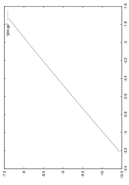
Figure 14. Error for the velocity ∥u−uh∥h\parallel\textbf{u}-\textbf{u}_{h}\parallel_{h} in Ωs\Omega_{s} ( log/log plot)
Refer to caption
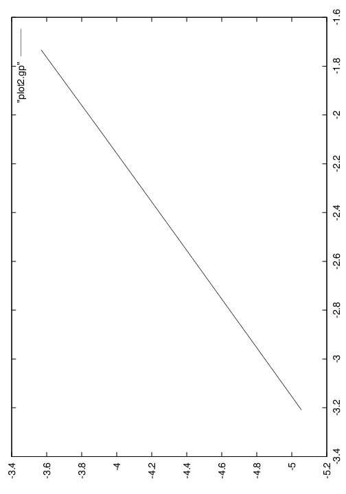
Figure 15. Error for the pressure ∥p−ph∥\parallel p-p_{h}\parallel in Ωs\Omega_{s} (log/log plot)
Refer to caption
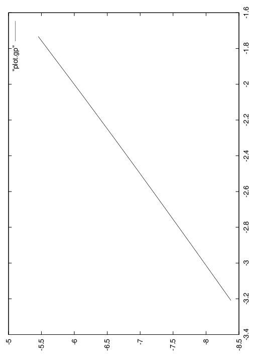
Figure 16. Error for the velocity ∥u−uh∥h\parallel\textbf{u}-\textbf{u}_{h}\parallel_{h} in Ωd\Omega_{d} (log/log plot)
Refer to caption
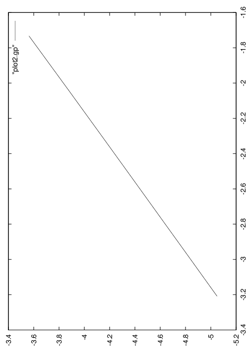
Figure 17. Error for the pressure ∥p−ph∥\parallel p-p_{h}\parallel in Ωd\Omega_{d} (log/log plot)
Refer to caption
Figure 18. The isovalue of the first velocity component u1u_{1} in Ωs\Omega_{s}.
Refer to caption
Figure 19. The isovalue of the second velocity component u2u_{2} in Ωs\Omega_{s}
Refer to caption
Figure 20. The isovalue of the first velocity component u1u_{1} in Ωd\Omega_{d}
Refer to caption
Figure 21. The isovalue of the second velocity component u2u_{2} in Ωd\Omega_{d}
Parameter hh o/o{}^{o}/_{o} of Coefs. ≠\neq 0
1/16 79.668827
1/22 66.405634
1/28 41.751001
1/34 28.652204
1/40 20.873193
1/46 15.879941
1/52 12.485349
1/58 10.073294
1/66 08.298201
1/70 06.954061
Table 1. Structure of rigidity Matrix on 1010 iterations.
Refer to caption
Figure 22. Component u1u_{1} in Ω\Omega.
Refer to caption
Figure 23. Component u2u_{2} in Ω\Omega.
Refer to caption
Figure 24. Pressure pp in Ω\Omega.
Refer to caption
Figure 25. Right-hand term f1f_{1} in Ωs\Omega_{s}.
Refer to caption
Figure 26. Right-hand term f2f_{2} in Ωs\Omega_{s}.
Refer to caption
Figure 27. Right-hand term k1k_{1} in Ωd\Omega_{d}.
Refer to caption
Figure 28. Right-hand term k2k_{2} in Ωd\Omega_{d}.

5. Conclusion

In this contribution, we investigated a new mixed finite element method to solve the Stokes-Darcy fluid flow model without introducing any Lagrange multiplier. We proposed a modification of the Darcy problem which allows us to apply a slight variant nonconforming Crouzeix-Raviart element to the whole coupled Stokes-Darcy problem. The proposed method is probably one the cheapest method for Discontinuous Galerkin (D​G)(DG) approximation of the coupled system, has optimal accuracy with respect to solution regularity, and has simple and straightforward implementations. Numerical experiments have been also presented, which confirm the excellent stability and accuracy of our method.

6. Acknowledgment

The author thanks Professor Emmanuel Creusé (University of Lille 1, France) for having sent us useful documents and for fruitful discussions concerning the numerical tests.

References

  • [1] T. Arbogast and D. Brunson. A computational method for approximating a Darcy-Stokes system governing a vuggy porous medium. Computational Geosciences, 11:207–218, 2007.
  • [2] M. G. Armentano and M. L. Stockdale. A unified mixed finite element approximations of the Stokes-Darcy coupled problem. Computers and Mathematics with Applications, https://doi.org/10.1016/j.camwa.2018.12.032, 2018.
  • [3] I. Babuška and G. Gatica. A residual-based a posteriori error estimator for the Stokes-Darcy coupled problem. SIAM J. Numer. Anal., 48:498–523, 2010.
  • [4] G. Beavers and D. Joseph. Boundary conditions at a naturally permeable wall. J. Fluid Mech., 30:197–207, 1967.
  • [5] S. Brenner. Korn’s inequalities for piecewise H1{H}^{1} vector fields. Math. Comput., 73:1067–1087, 2003.
  • [6] W. Chen and Y. Wang. A posteriori error estimate for H(div) conforming mixed finite element for the coupled Darcy-Stokes system. Journal of Computational and Applied Mathematics, 255:502–516, 2014.
  • [7] M. Crouzeix and P. Raviart. Conforming and nonconforming finite element methods for solving the stationary Stokes equations. Rev. Française Automat. Informat. Recherche Opérationnelle sér. Rouge, 7:33–75, 1973.
  • [8] M. Cui and N. Yan. A posteriori error estimate for the Stokes-Darcy system. Math. Meth. Appl. Sci., 34:1050–1064, 2011.
  • [9] M. Discacciati and A. Quarteroni. Navier-Stokes/Darcy coupling: Modeling, analysis, and numerical approximation. Rev. Math. Comput., 22:315–426, 2009.
  • [10] A. Ern. Aide-mémoire eléments finis. Dunod, Paris, ISBN 2 10 007303 6, 2005.
  • [11] H. Frederic and P. Olivier. Freefem++. http://www.freefem.org.
  • [12] J. Galvis and M. Sarkis. Nonconforming mortar discretization analysis for the coupling Stokes-Darcy equations. Electronic. Trans. Numer. Anal., 26:350–384, 2007.
  • [13] G. Gatica, R. Oyarzùa, and F.-J. Sayas. A residual-based a posteriori error estimator for a fully-mixed formulation of the Stokes-Darcy coupled problem. Comput. Methods Appl. Mech. Engrg., 200:1877–1891, 2011.
  • [14] G. N. Gatica, S. Meddahi, and R. Oyarzùa. A conforming mixed finite element method for the coupling of fluid flow with porous media flow. IMA J. Numer. Anal., 29:86–108, 2009.
  • [15] G.-N. Gatica, R. Oyarzùa, and F.-J. Sayas. Convergence of a family of galerkin discretizations for the Stokes-Darcy coupled proplem.
  • [16] V. Girault and P.-A. Raviart. Finite element methods for Navier-Stokes equations, Theory and algorithms, volume 5 of Springer, Berlin. In Computational Mathematics, 1986.
  • [17] F. Hecht. The mesh adapting software: bamg. INRIA report.http://www-c.inria.fr/gamma/cdrom/www/bamg/eng.htm, 1998.
  • [18] K. W. Houédanou, J. Adetola, and B. Ahounou. Residual-based a posteriori error estimates for a conforming finite element discretization of the Navier-Stokes/Darcy coupled problem. Journal of Pure and Applied Mathematics : Advances and Applications, 18(1):37–73, 2017.
  • [19] K. W. Houédanou and B. Ahounou. A posteriori error estimation for the Stokes-Darcy coupled problem on anisotropic discretization. Math. Meth. Appl. Sci., 2016. http://dx.doi.org/10.1002/mma.4261 (in press).
  • [20] W. Jäger and A. Mikelić. On the boundary conditions of the contact interface between a porous medium and a free fluid. Ann. Scuola Norm. Sup. Oisa Cl. Sci., 23:403–465, 1996.
  • [21] W. Jäger and A. Mikelić. On the interface boundary condition of Beavers, Joseph and Saffman. SIAM Journal on Applied Mathematics, 60:1111–1127, 2000.
  • [22] W. Jäger and A. Mikelić. On the interface boundary condition of Beavers, Joseph and Saffman. SIAM J. Appl. Math., 60:1111–1127, 2000.
  • [23] W. Jäger, A. Mikelić, and N. Neuss. Asymptotic analysis of the laminar visous flow over a porous bed. SIAM J. Sci. Comput., 22:2006–2028, 2001.
  • [24] R. Li, J. Li, Z. Chen, and Y. Gao. A stabilized finite element method based on two local gauss integrations for a coupled Stokes-Darcy problem. http://dx.doi.org/10.1016/j.cam.2015.06.014, 2015.
  • [25] K.-A. Mardal, X. Tai, and R. Winther. A robust finite element method for darcy-stokes flow. SIAM Journal on Numerical Analysis, 40:1605–1631, 2002.
  • [26] M. Mu and J. Xu. A two-grid method of a mixed Stokes-Darcy model for coupling fluid flow with porous media flow. SIAM Journal on Numerical Analysis, 45:1801–1813, 2007.
  • [27] S. Nicaise, B. Ahounou, and W. Houédanou. A residual-based posteriori error estimates for a nonconforming finite element discretization of the Stokes-Darcy coupled problem: Isotropic discretization. Afr. Mat., African Mathematical Union and Springer-Verlag Berlin Heidelberg: New York, 27(3):701–729 (2016), 2015.
  • [28] L. Payne and B. Straughan. Analysis of the boundary condition at the interface between a viscous fluid and a porous medium and related modeling questions. J. Math. Pures Appl., 77:317–354, 1998.
  • [29] B. Rivière and I. Yotov. Locally conservative coupling of Stokes and Darcy flows. SIAM J. Numer. Anal., 42:1959–1977, 2005.
  • [30] H. Rui and R. Zhang. A unified stabilized mixed finite element method for coupling Stokes and Darcy flows. Comput. Methods Appl. Mech. Engrg., 198:2692–2699, 2009.
  • [31] P. Saffman. On the boundary condition at the interface of a porous medium. Stud. Appl. Math., 1:93–101, 1971.
  • [32] D. Vassilev and I. Yotov. Coupling Stokes-Darcy flow with transport. SIAM J. Sci. Comput., 5:3661–3684, 2009.
  • [33] L. J. William, S. Friedhelm, and Y. Ivan. Coupling fluid flow with porous media flow. SIAM J. Numer. Anal., 40(6):2195–2218 (2003), 2002.
  • [34] J. Yu, M. A. A. Mahbub, F. Shi, and H. Zheng. Stabilized finite element method for the stationary mixed Stokes-Darcy problem. Advances in Diffference Equations, https:// doi.org/10.1186/s13662-018-1809-2346, 2018.