A way to generate poloidal (zonal) flow in the dynamics of drift (Rossby) waves

1. The quasi-geostrophic or Charney-Hasegawa-Mima (CHM) equation Charney 1948; Hasegawa and Mima 1977

is a basic model for several different phenomena, in particular, $1^{\ast}$ ocean dynamics Vallis 2006, $2^{\ast}$ tokamak plasmas Diamond et al. 2010; Horton 2012, and $3^{\ast}$ slow magneto-hydrodynamics in the ocean of the core Braginsky 2007 (in the latter case, instead of being the stream function, $\psi$ is the vertical component of the vector potential, so $-\psi_{y},\psi_{x}$ are the horizontal components of magnetic field Balk 2014).

In all these situations the generation of poloidal/zonal flow is important. In the first case emerging zonal flow limits the meridional transport. In the second case, poloidal flow limits the transport in the radial direction of a tokamak. In the third case, instead of zonal flow, we have generation of zonal magnetic field, important for dynamo theory.

Unlike cases $1^{\ast}$ and $3^{\ast}$, in the case $2^{\ast}$ we can actually change something; and this is the reason why the CHM equation is written here in the plasma notations (with radial $x$ and poloidal $y$ coordinates; units are chosen to make coefficients equal 1).

The present paper describes what increment/decrement could we add to the CHM equation in order to generate or to aid in the generation of poloidal flow (a transport barrier).

In the Fourier representation, the equation (1) — with the increments $\gamma_{\bf k}$ — becomes

where indices $\alpha,\beta$ (and later $\lambda,\mu,\nu$) stand for the corresponding wave vectors (${\bf k}_{\alpha},\ldots$); $d_{\alpha\beta}=d{\bf k}_{\alpha}\,d{\bf k}_{\beta}$.

is the dispersion law [wave vector ${\bf k}=(p,q)$, $k^{2}=p^{2}+q^{2}$]; the coupling kernel $W_{-{\bf k}\,\alpha\,\beta}=U_{-{\bf k}\,\alpha\,\beta}\;\delta(-{\bf k}+{\bf k}_{\alpha}+{\bf k}_{\beta})$,

2. The equation (1) is remarkable in the following sense Balk et al. 1991; Balk 1991. In addition to the energy and the momentum (the enstrpophy is their linear combination), this equation has an (independent) extra invariant, conserved adiabatically, i.e. approximately over long time. To see this, consider the quantity

with undetermined coefficient functions $X$ and $Y$ (without loss of generality, $Y$ is independent of the order of its indices, and $X$ is even, $X_{\bf k}=X_{-\bf k}$ since $\overline{\psi_{\bf k}}=\psi_{-{\bf k}}$). The time derivative of (5) due to the equation (2) is

Suppose the drift waves have small amplitudes and small increments: $\psi_{\bf k}=O(\epsilon)$ and $\gamma_{\bf k}=O(\epsilon)$, $\epsilon$ is a small parameter. $O(\epsilon^{3})$ terms in (6) would cancel if we chose

Without increment ($\gamma_{\bf k}\equiv 0$), we have $\dot{I}=O(\epsilon^{4})$, while $I=O(\epsilon^{2})$; integrating in time, we find $\Delta I\equiv I(t)-I(0)=O(\epsilon^{3})$ over long time $t=O(\epsilon^{-1})$. Notice that the $Y$-term in (5) has the same order $O(\epsilon^{3})$ as $\Delta I$, and so, the $Y$-term can be eventually discarded.

The above argument tacitly assumes that the expression (7) does not blow-up when its denominator vanishes. The latter condition turns out to be very restrictive Zakharov and Shul’man 1980, realizable only for some special functions $X_{\bf k}$.

If $X_{\bf k}=1+k^{2}$, then $Y\equiv 0$, and $I$ is the energy.

If $X_{\bf k}=k^{2}(1+k^{2})$, then $Y\equiv 0$, and $I$ is the enstrophy.

There is one choice with non-zero $Y$: $X_{\bf k}=\frac{(1+k^{2})^{2}}{q}\eta_{\bf k}$,

The requirement of no blow-up in (7) is reduced Balk and van Heerden 2006 to the conservation of function (9) in the 3-wave resonance interactions:

[recall that all three $W$ kernels in (7) contain the same delta function $\delta({\bf k}_{\lambda}+{\bf k}_{\mu}+{\bf k}_{\nu})$]. The condition (A way to generate poloidal (zonal) flow in the dynamics of drift (Rossby) waves) uniquely Balk and Ferapontov 1998 determines the function (9) — up to linear combinations: Obviously, any linear combination of functions ${\bf k},\Omega_{\bf k},\eta_{\bf k}$ is also conserved in the 3-wave resonance interactions. Actually, it is beneficial, instead of function $\eta_{\bf k}$, to consider function $\tilde{\eta}_{\bf k}=\eta_{\bf k}-2\sqrt{3}\,\Omega_{\bf k}$. This combination vanishes as $k\rightarrow\infty$, faster than $\eta_{\bf k}$ and $\Omega_{\bf k}$ separately; and this takes place along all directions in the ${\bf k}$-plane. The function $\tilde{\eta}_{\bf k}$ gives a well defined invariant, that holds in the physical space as well Balk and Yoshikawa 2009. The combination $\tilde{\eta}_{\bf k}$ also vanishes faster than $\eta_{\bf k}$ and $\Omega_{\bf k}$ separately, as $q\rightarrow 0$, for any $p$.

Thus, the equation (1) has three invariants:

We should keep in mind that the extra conservation holds only for weak nonlinearity, when $\epsilon$ is small enough, and the reminder $O(\epsilon^{4})$ in (8) can be neglected.

3. All three invariants (13) are positive-definite.

The presence of the extra invariant leads to essential conclusion about the energy transfer from the source (acting at some scale) to other scales Balk et al. 1991. The following argument Balk 2005 describes the emergence of poloidal flow.

Due to the enstrophy conservation, the energy from the source would transfer towards larger scales, i.e. towards the origin in the $k$-plane. Due to the extra conservation, the energy should concentrate near the $p$-axis, that correspond to the poloidal flow.

Indeed, Fig. 1 shows the contour plot of the ratio (14).

We see that $R_{\bf k}$ decreases when $k$ becomes large or when $q$ becomes small; more precisely,

So, if the energy from the source were transferred away from the $p$-axis, then the extra invariant would significantly increase: From the right upper corner (big $k$) in Fig. 1 to the left bottom corner (small $k$) the ratio $R$ changes by 9 orders of magnitude, provided the small wave vectors belong to the sector of polar angles $\theta\equiv\arctan(q/p)>30^{\circ}$. When $\theta$ decreases from $30^{\circ}$ to $0^{\circ}$, the ratio $R$ decreases to zero. So, the difference in scales (between the source scale and the big scale) should be large enough, to ensure the energy concentration near the $p$-axis.

This reasoning equally applies to the cascade (local in the ${\bf k}$-plane) or non-local energy transfer. So, the poloidal flow is always generated (without us doing anything).

However, there is a problem with this argument: It is hardly possible in practice, that the drift waves are weakly nonlinear in a wide range of scales. Usually, smaller scales are strongly nonlinear, while larger scales are weakly nonlinear (e.g. Rhines 1975). Below we present an argument, showing the possibility of zonal flow generation without wide range of scales. But we do need to arrange increment/decrement in certain special way.

This possibility is due to the fact that the contour lines in Fig. 1 have a “depression” in some region near the $q$-axis (away from the poloidal flow, corresponding to the $p$ axis): In this region, the ratio $R_{\bf k}$ is an increasing function of $p$ (while $q$ is fixed). This “depression” is hardly visible in Fig. 1.

4. Let there be a positive increment in a small neighborhood $B_{1}$ of some wave vector ${\bf k}_{1}$ and a decrement in a small neighborhood $B_{2}$ of some ${\bf k}_{2}$, while $\gamma_{\bf k}\equiv 0$ everywhere else. Consider positive quantities

According to (13),

here $E^{0},\Phi^{0},I^{0}$ are the initial values (at $t=0$) of the energy, enstrophy, extra invariant; their final values (at $t=\infty$) are $E^{\star},\Phi^{\star},I^{\star}$;  $R_{j}=R_{{\bf k}_{j}}\,(j=1,2)$. Slight difference between $k_{1}$ and $k_{2}$ (respectively, $R_{1}$ and $R_{2}$) could produce large difference between $\Phi^{0}$ and $\Phi^{\star}$ ($I^{0}$ and $I^{\star}$) if the time interval is long enough.

We want to generate significant amount of energy ($G_{1}>G_{2}$) and to have small amount of the extra invariant $I^{\star}\approx 0$. [Recall that the vanishing of the extra invariant requires vanishing of all drift waves besides the poloidal flow.] If $I^{\star}<I^{0}$, i.e. $R_{1}\,G_{1}-R_{2}\,G_{2}<0$, then

The condition (18) is implied by even less stringent requirement that the generated extra invariant per generated energy $\frac{R_{1}\,G_{1}-R_{2}\,G_{2}}{G_{1}-G_{2}}$ is less than $R_{1}$ or $R_{2}$.

We want to generate large-scale flow. In other words, the energy should concentrate in longer waves. The latter carry less enstrophy per energy than shorter waves. Thus, we should pump mostly energy and dissipate mostly enstrophy, i.e.

Formally, the condition (19) follows from the requirement that the generated enstrophy per generated energy $\frac{k_{1}^{2}\,G_{1}-k_{2}^{2}\,G_{2}}{G_{1}-G_{2}}$ is less than $k_{1}^{2}$ or $k_{2}^{2}$.

If (19) does not hold, $k_{1}>k_{2}$, then it is actually possible that the extra invariant becomes small, but the poloidal flow is not generated; this can happen because the ratio $R_{\bf k}$ quickly decreases as $k$ increases [see Fig. 1 and asymptotics (A way to generate poloidal (zonal) flow in the dynamics of drift (Rossby) waves)].

We want to generate poloidal flow, and so, we require ${\bf k}_{3}={\bf k}_{1}+{\bf k}_{2}$ be a purely polodal wave vector:

Figure 2 shows region of the ${\bf k}_{1}$-plane determined by the conditions (18) - (20), while $p_{3}$ is held fixed. These conditions automatically imply $k_{3}<k_{1}$. So, the wave ${\bf k}_{1}$ — pumped due to the positive increment — can decay into the waves ${\bf k}_{2}$ and ${\bf k}_{3}$ Gill 1974.

5. There is an additional bonus of condition (19): It implies that one can make numerical simulation with only few modes, as significantly shorter waves are not generated. The generation of much longer waves is also impossible if the scales corresponding to $k_{1},k_{2}$ are close to the size of the system.

Using this, we consider the simplified dynamics of only three waves Balk 2018 with wave vectors ${\bf k}_{3}=(1/2,0)$, ${\bf k}_{1}=(0,2)$ corresponding to the dot in Fig. 2, and ${\bf k}_{2}={\bf k}_{3}-{\bf k}_{1}$

$U_{1}=U_{{\bf k}_{1},{\bf k}_{3},-{\bf k}_{2}},\;U_{2}=U_{{\bf k}_{2},{\bf k}_{3},-{\bf k}_{1}},\;U_{3}=U_{{\bf k}_{3},{\bf k}_{1},{\bf k}_{2}},\\ \Omega_{j}=\Omega_{{\bf k}_{j}}\,(j=1,2,3),\;\;\gamma_{1}>0,\;\gamma_{2}<0$.

There is long history of modeling fusion plasmas by various small ode-systems (see Marcus et al. 2019; Rypina et al. 2007 and references cited therein).

Fig. 3 shows the emergence of poloidal flow in the model (A way to generate poloidal (zonal) flow in the dynamics of drift (Rossby) waves).

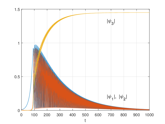
I performed simulations using MATLAB ode-solvers with decreased absolute and relative tolerances (‘AbsTol’ & ‘RelTol’). Instead of MATLAB default values ‘AbsTol’$=10^{-6}$ and ’RelTol’$=10^{-3}$, I used ‘AbsTol$=10^{-13}$ and ’RelTol’$=10^{-11}$. These are needed for validity of long-time simulations. I also checked that different ode-solvers produced indistinguishable results.

The relevance of these calculations to tokamak plasmas is due to the smallness in seconds of the time scale for drift waves. In particular, for ITER, the drift velocity is $v_{d}\sim 2$km/s and the ion inertial (Rossby) radius $\rho\sim 3$mm Horton and Benkadda 2015; therefore, the time scale is $\rho/v_{d}\sim(3/2)10^{-6}$s. So, dimensionless time $t=1000$ (the time-range in Fig. 3) corresponds to $1.5\times 10^{-3}$s; within a fraction of this time, the amplitude of the poloidal mode becomes significantly bigger than the amplitudes of the other two modes. The emergence of the poloidal flow would occur faster if the increment and decrement had bigger magnitudes.

6. If the emerging flow were not poloidal, it would be unstable with respect to decays into other waves. But poloidal flow is stable in the weak interaction limit Gill 1974. One can derive that the poloidal mode is stable if

i.e. the fluid velocity $v_{3}=ip_{3}\psi_{3}$, due to the poloidal wave, has smaller magnitude than the phase velocity of this wave. ¹¹ 1 Indeed, in the weak interaction limit, the instability of a Rossby wave ${\bf k}_{3}$ is the instability with respect to decays into a pair of waves, say ${\bf k}_{4}$ and ${\bf k}_{5}$, such that ${\bf k}_{3}={\bf k}_{4}+{\bf k}_{5},$ and $k_{3}$ is in between $k_{4}$ and $k_{5}$ Gill 1974. It is well known, that this instability does not take place if $\displaystyle D\equiv\omega^{2}/4-U_{4}U_{5}|\psi_{3}|^{2}>0,$ where $\omega=\Omega_{4}+\Omega_{5}\;(\Omega_{3}=0)$, and according to (4), $\displaystyle U_{4}=U({\bf k}_{4},{\bf k}_{3},-{\bf k}_{5})=p_{3}q_{5}(k_{3}^{2}-k_{5}^{2})/(1+k_{4}^{2}),$ $\displaystyle U_{5}=U({\bf k}_{5},{\bf k}_{3},-{\bf k}_{4})=p_{3}q_{4}(k_{3}^{2}-k_{4}^{2})/(1+k_{5}^{2}).$ Since $q_{4}+q_{5}=0$, $\displaystyle\omega=q_{4}\left(\frac{1}{1+k_{4}^{2}}-\frac{1}{1+k_{3}^{2}}\right)+q_{5}\left(\frac{1}{1+k_{5}^{2}}-\frac{1}{1+k_{3}^{2}}\right).$ By inequality between arithmetic and geometric means, $\displaystyle\left(\frac{\omega}{2}\right)^{2}$ $\displaystyle\geq$ $\displaystyle q_{4}q_{5}\frac{(k_{3}^{2}-k_{4}^{2})(k_{3}^{2}-k_{5}^{2})}{(1+k_{4}^{2})(1+k_{5}^{2})(1+k_{3}^{2})^{2}},\quad\Longrightarrow$ $\displaystyle D$ $\displaystyle\geq$ $\displaystyle q_{4}^{2}\frac{(k_{4}^{2}-k_{3}^{2})(k_{3}^{2}-k_{5}^{2})}{(1+k_{4}^{2})(1+k_{5}^{2})}\left\{\frac{1}{(1+k_{3}^{2})^{2}}-p_{3}^{2}|\psi_{3}|^{2}\right\}.$ So, $D>0$ if the condition (22) holds.

This stability in the weak interaction limit matches the argument based on the extra invariant that requires weak nonlinearity, as well.

The considerations in the present paper can be extended to the dynamics in different equations; it is only important that such an equation has dispersion law (3) and possesses Hamiltonian structure, e.g. see Qi and Majda 2019.

References

- Charney (1948) J. G. Charney, Geophys. Publ. Oslo 17, 1 (1948).
- Hasegawa and Mima (1977) A. Hasegawa and K. Mima, Phys. Rev. Lett. 39, 205 (1977).
- Vallis (2006) G. K. Vallis, Atmospheric and Oceanic Fluid Dynamics. Fundamentals and Large-scale Circulation (Cambridge, 2006).
- Diamond et al. (2010) P. H. Diamond, S.-I. Itoh, and K. Itoh, Modern Plasma Physics, Vol. 1 (Cambridge University Press, 2010).
- Horton (2012) W. Horton, Turbulent Transport in Magnetized Plasmas (World Scientific, 2012).
- Braginsky (2007) S. I. Braginsky, Earth and Planet. Sci. Lett. 253, 507 (2007).
- Balk (2014) A. M. Balk, ApJ 796, 143 (8pp) (2014).
- Balk et al. (1991) A. M. Balk, S. V. Nazarenko, and V. E. Zakharov, Phys. Lett. A 152, 276 (1991).
- Balk (1991) A. M. Balk, Phys. Lett. A 155, 20 (1991).
- Zakharov and Shul’man (1980) V. E. Zakharov and E. I. Shul’man, Physica D 10, 192 (1980).
- Balk and van Heerden (2006) A. M. Balk and F. van Heerden, Physica D 223, 109 (2006).
- Balk and Ferapontov (1998) A. M. Balk and E. V. Ferapontov, in Nonlinear waves and weak turbulence, edited by V. E. Zakharov (Amer. Math. Soc. Trans. Ser. 2, vol. 182, 1998) pp. 1–30.
- Balk and Yoshikawa (2009) A. M. Balk and T. Yoshikawa, Physica D 238, 384 (2009).
- Balk (2005) A. M. Balk, Phys. Lett. A 345, 154 (2005).
- Rhines (1975) P. B. Rhines, J. Fluid Mech. 69, 417 (1975).
- Gill (1974) A. Gill, Geophysical Fluid Dynamics 6, 29 (1974).
- Balk (2018) A. M. Balk, Phys. Rev. E 98, 062208 (2018).
- Marcus et al. (2019) F. A. Marcus, M. Roberto, I. L. Caldas, K. C. Rosalem, and Y. Elskens, Physics of Plasmas 26, 022302 (2019), https://doi.org/10.1063/1.5071437 .
- Rypina et al. (2007) I. I. Rypina, M. G. Brown, F. J. Beron-Vera, H. Kocak, M. J. Olascoaga, and I. A. Udovydchenkov, Phys. Rev. Lett. 98, 104102 (2007).
- Horton and Benkadda (2015) W. Horton and S. Benkadda, ITER Physics (World Scientific Publishing Company, 2015).
- (21)
Indeed, in the weak interaction limit, the instability of a
Rossby wave is the instability with respect to decays
into a pair of waves, say and , such
that and is
in between and Gill 1974. It is well known, that this
instability does not take place if
where , and according to (4),
Since ,
By inequality between arithmetic and geometric means,
So, if the condition (22) holds. - Qi and Majda (2019) D. Qi and A. J. Majda, arXiv e-prints , arXiv:1901.08590 (2019), arXiv:1901.08590 [physics.plasm-ph] .