Subradiant Dimer Excitations of Emitter Chains Coupled to a 1D Waveguide
Abstract
This Letter shows that chains of optical or microwave emitters coupled to a 1D waveguide support subradiant states with close pairs of excited emitters, which have longer lifetimes than even the most subradiant states with only a single excitation. Exact, analytical expressions for non-radiative excitation dimer states are obtained in the limit of infinite chains. To understand the mechanism underlying these states, we present a formal equivalence between subradiant dimers and single localized excitations around a chain defect (unoccupied site). Our analytical mapping permits extension to emitter chains coupled to the 3D free space vacuum field.
Subradiance, the cooperative inhibition of spontaneous emission from an ensemble of emitters, has been pursued since the seminal work by Dicke Dicke 1954 and has been observed only recently in atomic gases Guerin et al. 2016; Weiss et al. 2018 and in metamaterial arrays Jenkins et al. 2017. Applications in quantum information processing Paulisch et al. 2016 motivate the studies of collective light-matter interactions, including the subradiant excitations of one-dimensional (1D) emitter chains Haakh et al. 2016; Ruostekoski and Javanainen 2016; Ruostekoski and Javanainen 2017; Zoubi 2014; Kornovan et al. 2016; Sutherland and Robicheaux 2016; Olmos et al. 2013; Bettles et al. 2016; Jen et al. 2016; Asenjo-Garcia et al. 2017; Albrecht et al. 2019; Henriet et al. 2019; Zhang and Mølmer 2019; Solano et al. 2017; Paulisch et al. 2016; Asenjo-Garcia et al.; Kornovan et al.; Zhang et al.; Wang and Zhao 2018, 2D arrays Perczel et al. 2017; Facchinetti et al. 2016; Guimond et al. 2019 and other geometries Needham et al.; Moreno-Cardoner et al. 2019; Lee and Lee 1973. The phenomenon of subradiance is found to occur due to different mechanisms, e.g., spin waves with wave numbers outside the “light line” Asenjo-Garcia et al. 2017, entangled states between remote ensembles Guimond et al. 2019; Needham et al.; Moreno-Cardoner et al. 2019, subradiant edge states enabled by nontrivial topology Perczel et al. 2017; Zhang et al.; Wang and Zhao 2018, etc. However, these results were so far restricted to ensembles with only a single excitation while subradiant states with more excitations have remained largely unexplored.
An exception is the so-called fermionic multi-excitation subradiant states in 1D systems Albrecht et al. 2019; Asenjo-Garcia et al. 2017; Henriet et al. 2019. While one might expect emitter saturation to play only a perturbative role in the few-excitation scenarios Porras and Cirac 2008, it enforces an equivalence between the multi-excitation subradiant states and the Tonks-Girardeau gas of hard core bosons Zhang and Mølmer 2019. This suggests a class of subradiant states with state amplitudes which are anti-symmetric combinations of the one-excitation subradiant states.
However, numerical analyses of emitter chains coupled to a 1D waveguide reveal the existence of another family of subradiant states with entirely different properties, see Zhang and Mølmer 2019 and (sp, Sec. A). In this Letter, we first numerically demonstrate and assess the extraordinary properties of subradiant states with very close pairs of excited emitters, i.e., subradiant dimers. In particular, we find that for specific distances between the excited emitters their radiative lifetimes can be longer than the fermionic states and even than the most long-lived one-excitation states :aa. Then, we present an analytical treatment that explains the confinement mechanism that leads to the subradiant dimers by a mapping to the localized subradiant excitation near an unoccupied site (defect) in the chain. This confinement-localization mapping is valid under more general conditions and allows extension of our analysis, e.g., to emitter chains coupled to the 3D free space quantized field.

Spin Model.
Consider a chain of two-level emitters equally spaced by the distance , as illustrated in Fig. 1(a). Each emitter has a ground state and an excited state with transition frequency . The emitters are coupled to a 1D waveguide that supports light modes with a linear dispersion relation. Using the Born-Markov approximation, the waveguide modes can be eliminated to yield an effective theory for the emitters Dung et al. 2002, which entails a non-Hermitian infinite-range spin-spin interaction Hamiltonian Chang et al. 2012; Caneva et al. 2015; Roy et al. 2017
| (1) |
The bare excitation energies of the individual emitters are not included, is the decay rate of an individual emitter coupled to the waveguide, is the wave number of the waveguide mode resonant with , is the position coordinate of the emitter and . In a perfect experimental implementation of (1) should dominate all other decay processes, as in photonic crystal waveguides Zang et al. 2016; Chang et al. 2018 and superconducting qubits coupled to transmission lines Astafiev et al. 2010; Hoi et al. 2011; Van Loo et al. 2013; Mirhosseini et al. 2019.
In the Monte Carlo wave function formalism Mølmer et al. 1993, the state of the emitter chain evolves under Eq. (1), interrupted by stochastic quantum jumps representing spontaneous emission of a photon. The jump rate makes a system prepared in a right eigenstate of maintain its excitation with a probability that decays with twice the negative imaginary part of the corresponding eigenvalue. In this work, we obtain these eigenstates by the exact diagonalization of with use of the SLEPc (Scalable Library for Eigenvalue Problem Computations) Hernandez et al. 2005.
Subradiant dimer excited states.
We focus on the two-excitation subspace of eigenstates of , for lattices with . This Hilbert space is spanned by states where the and emitters are excited. As we illustrate in Fig. 1, by numerical diagonalization of we find subradiant dimer states with delocalized center of mass and well-defined distance between the excitations. To understand the appearance of these states and their properties, we introduce basis states,
| (2) |
with center-of-excitation wave number and spatial separation between the excitations. In a finite chain, is not conserved but distributions resembling standing waves appear due to the boundary conditions at the chain ends. The expansion of the identified type-I dimers on the basis states (2) have wave numbers . For infinite chains, becomes a good quantum number and the type-I dimers can expressed as , where , see (sp, Sec. B). This implies a probability distribution for the separation between the excitations
| (3) |
with the dominant amplitude on , see Fig. 1(b). For the type-II dimers identified, , and on an infinite chain the amplitudes on odd values of vanish and the state can be expressed as . The summation includes only the even values of , and . This implies a distribution for even valued separations
| (4) |
with the dominant amplitude on , see Fig. 1(c). These dimers are perfectly subradiant with vanishing decay rates on infinite chains, i.e., the corresponding eigenvalues of are real. In (sp, Sec. B), we derive the asymptotic eigenvalues of the two types of dimers, viz., and , and numerically obtain their corrections on a finite chain. Knowing these asymptotic values allows efficient search for the eigenstates for a finite chain with a large number of emitters by the Krylov-Schur algorithm Stewart 2002 with the shift-and-invert method Saad 2011.
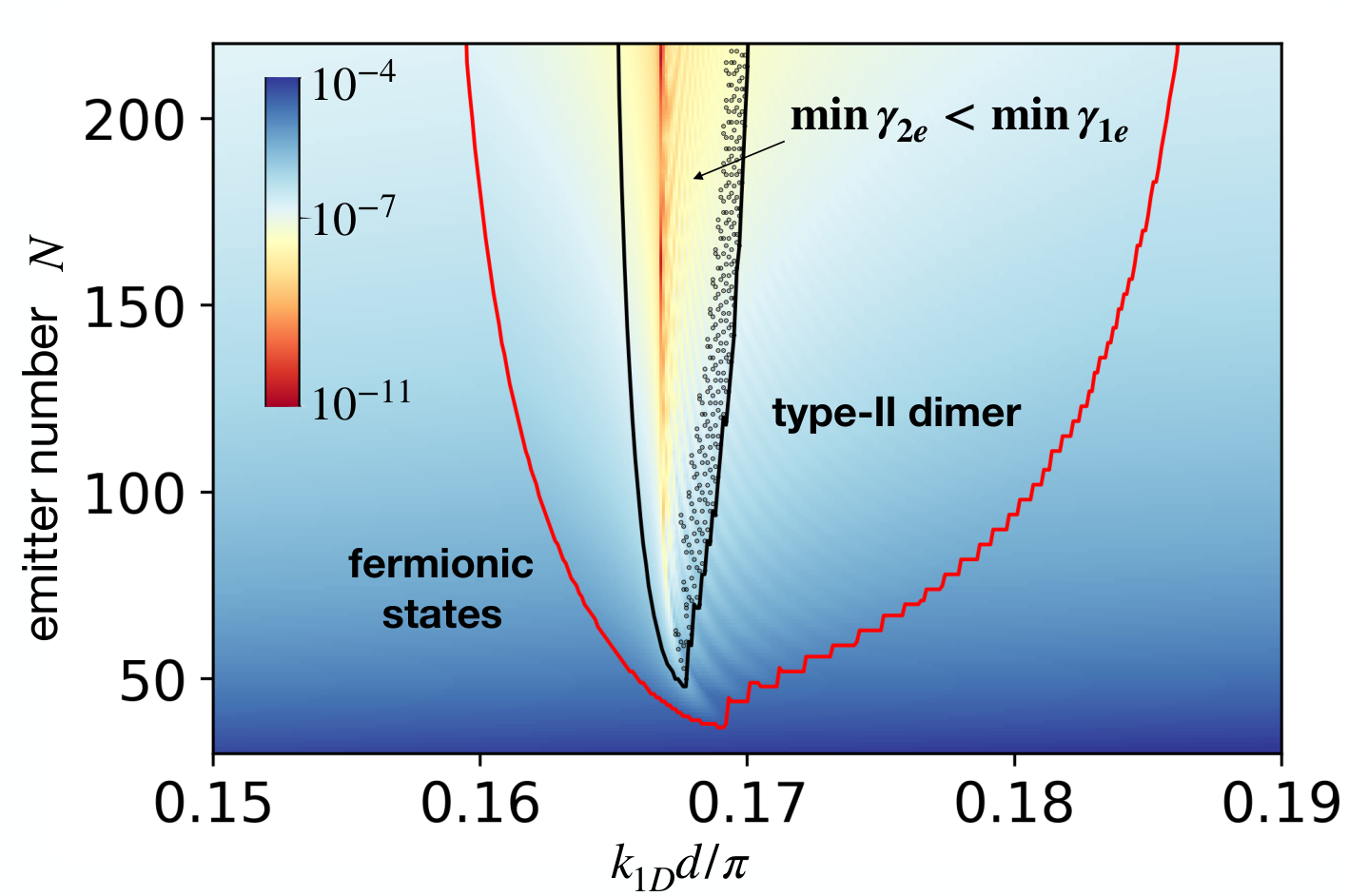

The dimers on finite chains have small but finite decay rates. We find that the minimal decay rates of the most subradiant type-I states scale asymptotically as nearly , see (sp, Sec. C). However, the type-II states show longer lifetimes and a more complex behaviour. The decay rate of the most subradiant type-II dimers is shown versus and in Fig. 2, where a narrow region between and is distinctively subradiant. Moreover, fringe textures are seen to the right hand side of that region. We compare the minimal decay rates of type-II dimers with those of the most subradiant fermionic states and one-excitation states, and obtain the critical parameters of and shown by the red and black boundary curves in Fig. 2. Specifically, Fig. 2 demonstrates that the type-II dimer can be more subradiant than the fermionic states, and even the one-excitation states. This observation disproves an unwritten orthodoxy that states with more excitations have shorter lifetimes, being true, for example, for the fermionic states that decay with the sum of their one-excitation constituent decay rates Asenjo-Garcia et al. 2017; Albrecht et al. 2019; Henriet et al. 2019. Fig. 2 shows that a short chain with emitters is sufficient to observe the even more subradiant dimer states, in the case of .
To study the extremely subradiant region in more detail, we plot decay rates of the most subradiant type-II dimers for a few values of in Fig. 3(a). A sharp dip in decay rates appears around and a magnified view of the interval shows the fringe textures observed in Fig. 2. The robustness of the results to position disorder is discussed in (sp, Sec. D). In Fig. 3(b), we observe different scalings of the decay rate with for different values of . Around , the decay rates thus fall off faster than and show oscillations breaking the conventional monotonicity with . For near , the decay rate is weakly modulated with a period of 4, see insert in Fig. 3(b): adding 4 emitters makes the chain longer by half a resonant wavelength.
When , Eq. (4) vanishes so that amplitudes of are completely suppressed. On infinite chains this state is an eigenstate of both the centre-of-excitation wave number, equivalent to a total momentum, , and the relative position coordinate, , i.e., it is an implementation of the Einstein-Podolsky-Rosen state Einstein et al. 1935. A similar state is found for the type-I dimer for .
Confinement-localization mapping.
The Hamiltonian Eq. (1) does not provide any direct evidence for the emergence of the subradiant dimer states, and neither does our analysis based on the Holstein-Primakoff transformation Zhang and Mølmer 2019. Here we provide the physical mechanism leading to the long lived excitation dimers.
Applying on the ansatz of Eq. (2) yields
| (5) |
It separates into contributions preserving , i.e., the matrix defined by elements
| (6) |
and remaining terms, denoted by “tails” that break the conservation of , see (sp, Sec. E). The “tails” vanish when . Thus the Hamiltonian acting on the relative position eigenstates is essential for the formation of dimers and must explain their vanishing decay rates on infinite chains.
Our key insight is that the eigenstates of can be uniquely mapped to the even-parity eigenstates of a Hamiltonian with matrix elements
| (7) |
where attain both positive and negative values . As shown in (sp, Sec. F), for an eigenstate of (with eigenvalue ), there is a corresponding even-parity eigenstate (unnormalized) of with the eigenvalue that satisfies for indices .
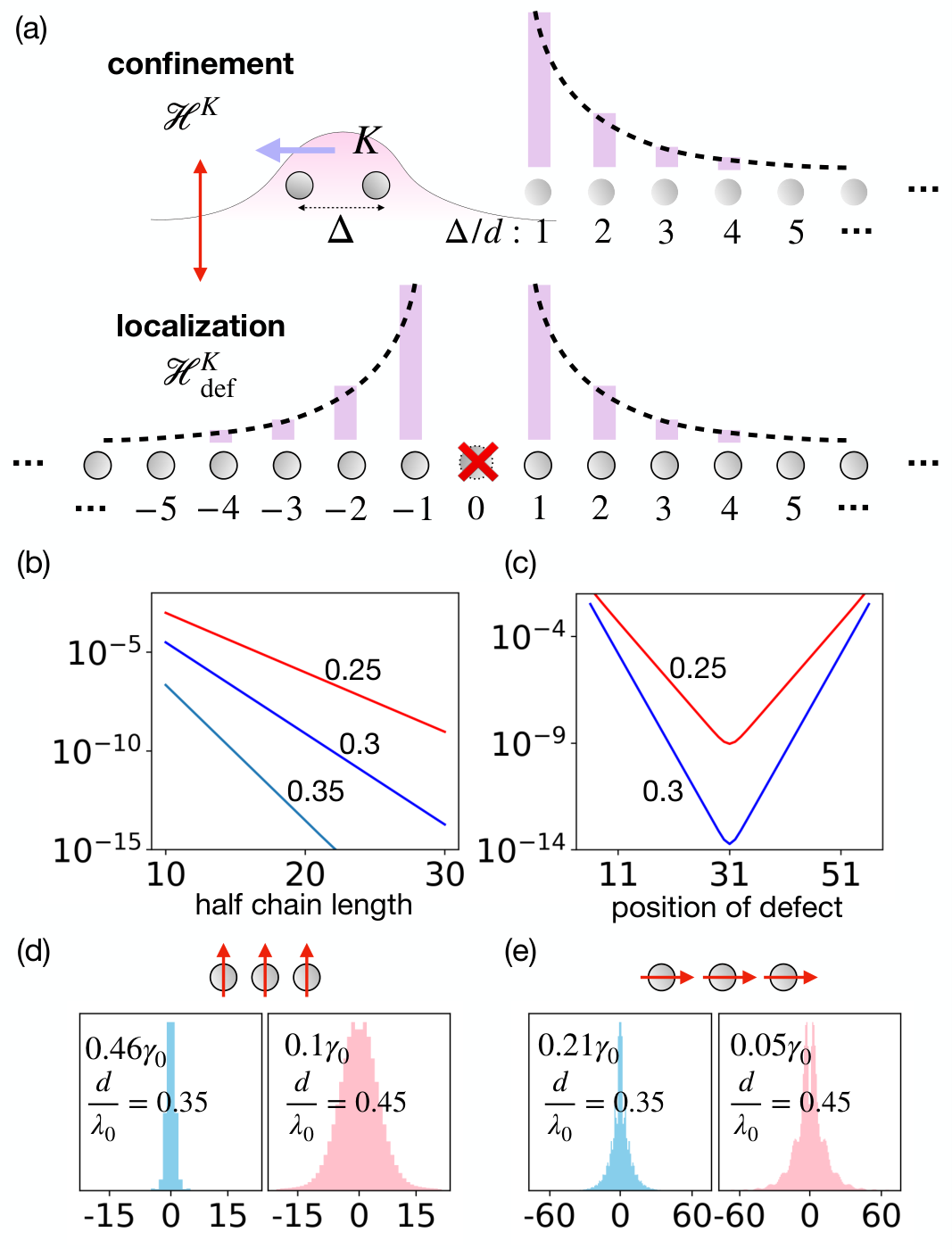
The above mapping implies that, the dimer state is equivalent to an eigenstate of the Hamiltonian , describing a single excitation localized around a defect (unoccupied site) at , as illustrated in Fig. 4(a). Actually for the case of , is just the defect version of Eq. (1). The localized defect modes have analytical solutions elaborated in (sp, Sec. G). On an infinite chain, the localized eigenstate of can be written as with . This is in agreement with the spatial factor Eq. (3) found for the type-I dimers. The eigenvalue of for the localized state is , exactly half of that of the type-I dimer , as predicted by the confinement-localization mapping. The case of (type-II dimers) is equivalent to the case of (sp, Sec. H), up to alternating sign flips and the replacement of . This equivalence explains the resemblance between Eqs. (3) and (4), and between the eigenvalues and .
The excitation of an emitter blocks further excitation and the dimer state is stable because each excitation serves as a defect supporting the localization of the other one. For finite chains, as shown in Fig. 4(b) the localized state around a defect has a decay rate suppressed exponentially in the emitter number , and if the defect is not at the chain center, the decay rate is determined by the length of the shorter subchain, see Fig. 4(c). This dependence is much faster than the scaling on chains free from defects Asenjo-Garcia et al. 2017; Albrecht et al. 2019; Henriet et al. 2019; Zhang and Mølmer 2019 and it comes about because the localized state is a superposition of a left and a right excited subchain. Their destructive interference results in the extreme subradiance, seen also in Refs. Guimond et al. 2019; Needham et al.; Moreno-Cardoner et al. 2019.
The finite size effects shown in Figs. 2 and 3 are due to the “tails” of Eq. (5). Since the states have finite width of , the “tails” is restricted to a short section of length at each end, but their complicated expression (sp, Sec. E) prevents analytical solution. We may, however, infer that the dimers become seriously affected at the chain ends, and hence an interplay between the length of the chain and the bond-length of the dimer may be responsible for the periodic oscillations seen in Fig. 3(b) and the fringe texture seen in Fig. 2. The strong dependence of the decay rates on the emitter separation might be equivalent to the observation, see Ref. Kornovan et al. of special emitter distances leading to extraordinary (single excitation) subradiant states.
Universality.
The mapping between confinement and localization can be extended by linearity to Hamiltonians written as , where is an integral measure over the variable and refers to Eq. (1). This for example covers 1D emitter chains coupled with 3D free space modes where is given in Ref. Zhang and Mølmer 2019. Also here, localized subradiant states will exist, and we show their excitation amplitude in Fig. 4(d,e) (see phase profiles in (sp, Sec. I)), for emitters polarized both transverse and parallel to the chain. In contrast to the 1D waveguide, these localized states have finite decay rates in the infinite chain limit. Due to the mapping, we can conclude that subradiant excitation dimers exist and that they have intrinsic finite decay rates also in the limit of infinite chains.
Conclusion and discussion.
In this Letter, we have introduced subradiant excited dimers of emitter chains coupled to a 1D waveguide. We showed that such (type-II) dimers can be more subradiant than even the longest lived one-excitation states of the system. Their decay rates show unusual dependence, including non-monotonic wiggles, as function of when is slightly larger than . We identify the intrinsic emitter saturation and the resulting emergence of mutual defect modes as the cause of the long lived dimer states, and we use a rigorous mapping between confinement and localization to obtain their physical properties. This mapping is valid under general conditions and gives access to the properties of similar states of emitter chains decaying into 3D free space field modes.
We propose to verify the predictions experimentally, and to address single excited states around defects, e.g., by exciting emitters around a missing or suitably perturbed site, and waiting for excitation amplitudes on orthogonal excitation modes to decay. To verify the dimer subradiant states, one would excite a system uniformly, but one may exploit interactions to facilitate correlated excitation of dimers within certain distance ranges Douglas et al. 2016, and thus maximize the overlap with the long lived states identified in this Letter. Other efficient ways to couple the bound states or localized states may be mediated by ancillary emitters distributed off the 1D lattice sites Mirhosseini et al. 2019; González-Tudela et al. 2015. Finally, we imagine that our method to formally map doubly excited states on localized states around defects may become a useful ingredient in other lattice models and contribute to the analysis of other quasiparticle confinement phenomena, cf., recent findings in Ising spin chains with long-range interactions Liu et al. 2019.
Acknowledgements.
This work was supported by the Villum Foundation, the European Unions Horizon 2020 research and innovation program (Grant No. 712721, NanOQTech), and the EuropeanUnion FETFLAG program (Grant No. 820391, SQUARE). The numerical results were obtained at the Center for Scientific Computing, Aarhus University.References
- Dicke (1954) R. H. Dicke, Phys. Rev. 93, 99 (1954).
- Guerin et al. (2016) W. Guerin, M. O. Araújo, and R. Kaiser, Phys. Rev. Lett. 116, 083601 (2016).
- Weiss et al. (2018) P. Weiss, M. O. Araújo, R. Kaiser, and W. Guerin, New J. Phys. 20, 063024 (2018).
- Jenkins et al. (2017) S. D. Jenkins, J. Ruostekoski, N. Papasimakis, S. Savo, and N. I. Zheludev, Phys. Rev. Lett. 119, 053901 (2017).
- Paulisch et al. (2016) V. Paulisch, H. Kimble, and A. González-Tudela, New J. Phys. 18, 043041 (2016).
- Haakh et al. (2016) H. R. Haakh, S. Faez, and V. Sandoghdar, Phys. Rev. A 94, 053840 (2016).
- Ruostekoski and Javanainen (2016) J. Ruostekoski and J. Javanainen, Phys. Rev. Lett. 117, 143602 (2016).
- Ruostekoski and Javanainen (2017) J. Ruostekoski and J. Javanainen, Phys. Rev. A 96, 033857 (2017).
- Zoubi (2014) H. Zoubi, Phys. Rev. A 89, 043831 (2014).
- Kornovan et al. (2016) D. F. Kornovan, A. S. Sheremet, and M. I. Petrov, Phys. Rev. B 94, 245416 (2016).
- Sutherland and Robicheaux (2016) R. T. Sutherland and F. Robicheaux, Phys. Rev. A 94, 013847 (2016).
- Olmos et al. (2013) B. Olmos, D. Yu, Y. Singh, F. Schreck, K. Bongs, and I. Lesanovsky, Phys. Rev. Lett. 110, 143602 (2013).
- Bettles et al. (2016) R. J. Bettles, S. A. Gardiner, and C. S. Adams, Phys. Rev. A 94, 043844 (2016).
- Jen et al. (2016) H. H. Jen, M.-S. Chang, and Y.-C. Chen, Phys. Rev. A 94, 013803 (2016).
- Asenjo-Garcia et al. (2017) A. Asenjo-Garcia, M. Moreno-Cardoner, A. Albrecht, H. J. Kimble, and D. E. Chang, Phys. Rev. X 7, 031024 (2017).
- Albrecht et al. (2019) A. Albrecht, L. Henriet, A. Asenjo-Garcia, P. B. Dieterle, O. Painter, and D. E. Chang, New J. Phys. 21, 025003 (2019).
- Henriet et al. (2019) L. Henriet, J. S. Douglas, D. E. Chang, and A. Albrecht, Phys. Rev. A 99, 023802 (2019).
- Zhang and Mølmer (2019) Y.-X. Zhang and K. Mølmer, Phys. Rev. Lett. 122, 203605 (2019).
- Solano et al. (2017) P. Solano, P. Barberis-Blostein, F. K. Fatemi, L. A. Orozco, and S. L. Rolston, Nat. Commun. 8, 1857 (2017).
- (20) A. Asenjo-Garcia, H. J. Kimble, and D. E. Chang, arXiv:1906.02204 .
- (21) D. F. Kornovan, N. V. Corzo, J. Laurat, and A. S. Sheremet, arXiv:1906.07423 .
- (22) A. Zhang, X. Chen, V. V. Yakovlev, and L. Yuan, arXiv:1907.07252 .
- Wang and Zhao (2018) B. X. Wang and C. Y. Zhao, Phys. Rev. A 98, 023808 (2018).
- Perczel et al. (2017) J. Perczel, J. Borregaard, D. E. Chang, H. Pichler, S. F. Yelin, P. Zoller, and M. D. Lukin, Phys. Rev. Lett. 119, 023603 (2017).
- Facchinetti et al. (2016) G. Facchinetti, S. D. Jenkins, and J. Ruostekoski, Phys. Rev. Lett. 117, 243601 (2016).
- Guimond et al. (2019) P.-O. Guimond, A. Grankin, D. V. Vasilyev, B. Vermersch, and P. Zoller, Phys. Rev. Lett. 122, 093601 (2019).
- (27) J. A. Needham, I. Lesanovsky, and B. Olmos, arXiv:1905.00508 .
- Moreno-Cardoner et al. (2019) M. Moreno-Cardoner, D. Plankensteiner, L. Ostermann, D. E. Chang, and H. Ritsch, Phys. Rev. A 100, 023806 (2019).
- Lee and Lee (1973) P. S. Lee and Y. C. Lee, Phys. Rev. A 8, 1727 (1973).
- Porras and Cirac (2008) D. Porras and J. I. Cirac, Phys. Rev. A 78, 053816 (2008).
- (31) Supplemental Material.
- (32) This is reminiscent of the recent theoretical discovery of a range of different power law dependences of the decay rates of single excitation states for very specific values of the atomic distances Kornovan et al..
- Dung et al. (2002) H. T. Dung, L. Knöll, and D.-G. Welsch, Phys. Rev. A 66, 063810 (2002).
- Chang et al. (2012) D. E. Chang, L. Jiang, A. Gorshkov, and H. Kimble, New J. Phys. 14, 063003 (2012).
- Caneva et al. (2015) T. Caneva, M. T. Manzoni, T. Shi, J. S. Douglas, J. I. Cirac, and D. E. Chang, New J. Phys. 17, 113001 (2015).
- Roy et al. (2017) D. Roy, C. M. Wilson, and O. Firstenberg, Rev. Mod. Phys. 89, 021001 (2017).
- Zang et al. (2016) X. Zang, J. Yang, R. Faggiani, C. Gill, P. G. Petrov, J.-P. Hugonin, K. Vynck, S. Bernon, P. Bouyer, V. Boyer, and P. Lalanne, Phys. Rev. Applied 5, 024003 (2016).
- Chang et al. (2018) D. E. Chang, J. S. Douglas, A. González-Tudela, C.-L. Hung, and H. J. Kimble, Rev. Mod. Phys. 90, 031002 (2018).
- Astafiev et al. (2010) O. Astafiev, A. Zagoskin, A. Abdumalikov, Y. Pashkin, T. Yamamoto, K. Inomata, Y. Nakamura, and J. Tsai, Science 327, 840 (2010).
- Hoi et al. (2011) I.-C. Hoi, C. M. Wilson, G. Johansson, T. Palomaki, B. Peropadre, and P. Delsing, Phys. Rev. Lett. 107, 073601 (2011).
- Van Loo et al. (2013) A. F. Van Loo, A. Fedorov, K. Lalumière, B. C. Sanders, A. Blais, and A. Wallraff, Science 342, 1494 (2013).
- Mirhosseini et al. (2019) M. Mirhosseini, E. Kim, X. Zhang, A. Sipahigil, P. B. Dieterle, A. J. Keller, A. Asenjo-Garcia, D. E. Chang, and O. Painter, Nature 569, 692 (2019).
- Mølmer et al. (1993) K. Mølmer, Y. Castin, and J. Dalibard, J. Opt. Soc. Am. B 10, 524 (1993).
- Hernandez et al. (2005) V. Hernandez, J. E. Roman, and V. Vidal, ACM Trans. Math. Software 31, 351 (2005).
- Stewart (2002) G. Stewart, SIAM J. Matrix Anal. Appl. 23, 601 (2002).
- Saad (2011) Y. Saad, Numerical Methods for Large Eigenvalue Problems (Society for Industrial and Applied Mathematics, 2011).
- Einstein et al. (1935) A. Einstein, B. Podolsky, and N. Rosen, Phys. Rev. 47, 777 (1935).
- Douglas et al. (2016) J. S. Douglas, T. Caneva, and D. E. Chang, Phys. Rev. X 6, 031017 (2016).
- González-Tudela et al. (2015) A. González-Tudela, V. Paulisch, D. E. Chang, H. J. Kimble, and J. I. Cirac, Phys. Rev. Lett. 115, 163603 (2015).
- Liu et al. (2019) F. Liu, R. Lundgren, P. Titum, G. Pagano, J. Zhang, C. Monroe, and A. V. Gorshkov, Phys. Rev. Lett. 122, 150601 (2019).
I Supplemental Material
I.1 A. Distributions of the eigenvalues in the two-excitation sector
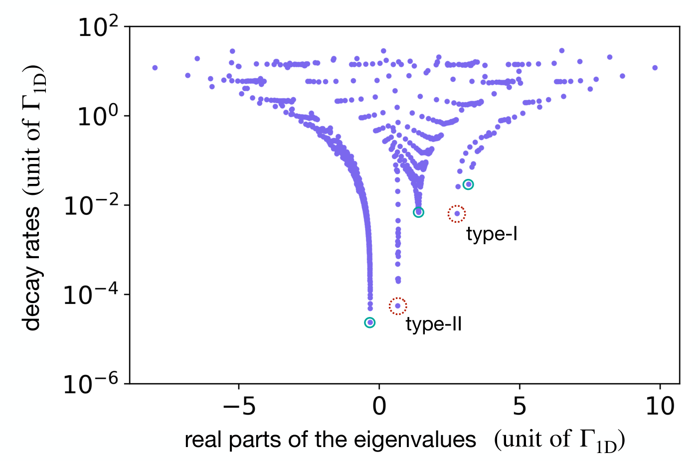
The fermionic states and the dimers constitute all the subradiant states in the two-excitation sector. This is verified by Fig. 1, where we show all the eigenvalues of for a chain of emitters coupled to a 1D waveguide with . In Fig. 1 five branches of subradiant states can be clearly identified. For the three branches of fermionic states, their asymptotic eigenvalues can be obtained from the supplemental material (Sec. A) of Ref. Zhang and Mølmer 2019. The asymptotic eigenvalues of the dimers are given in the main text and will be derived below in Sec. B.
I.2 B. Asymptotic eigenvalues of the dimers

In the limit of infinite chains, the most subradiant states have vanishing decay rates so that the corresponding eigenvalues are real. Analytical expressions of the asymptotic values can be obtained both from [Eq. (6) of the main text] and from (see Sec. F).
For the type-I dimers, applying on yields
| (1) |
where the coefficients are
| (2a) | |||
| (2b) | |||
| (2c) |
Suppose that has a positive imaginary part and is sufficiently large so that . This implies that and if we can find a value of so that , the corresponding is an eigenstate of . For large , this leads to the equation
| (3) |
The solution is . Substituting this into the expression for yields the real eigenvalue . In Fig. 2, we plot the deviations of energy levels of the dimers from their asymptotic values.
Counterparts of the type-II dimers can be obtained in the same way. One can also obtain them by using the equivalence between the two types of dimers as presented in Sec. H of this Supplemental Material.
I.3 C. Decay rates of the type-I dimers
The decay rates of the most subradiant type-I dimer states versus emitter number and are plotted in Fig. 3. Compared with the results for the type-II states, shown in the main text, the curves are free from dips and wiggles.

I.4 D. Robustness against spatial disorder
In this section, we examine the influence of disorder of the spatial positions of the emitters. It is conceivable that for weak disorder, the eigenstates are only slightly perturbed, while for more significant disorder, the system may display new physics, such as Anderson localization effects.
We restrict ourselves here to the situation of weak disorder. Then the position of each emitter is assumed to be shifted randomly by a distance uniformly distributed in a small interval . We show the decay rates of the most subradiant type-II dimer as a function of in Fig. 4 for a number of random realizations of the disorder. Our simulations show that the dip near is robust against the disorder, and that disorder can even lead to further suppression of the decay rates.

I.5 E. Full expression of terms omitted in Eq. (5) of the main text
The omitted “tails” are expressed as
| (4) | ||||
where is the state where no emitters are excited, , and the foot indices and restrict the summation over sites to the intervals and , respectively. For dimer states dominated by small values of , the “tail” terms are well restricted to the ends of the chain.
I.6 F. Mapping from to
The one-to-one correspondence between the eigenstates of and the even eigenstates of can be understood from the following simple observation.
From Eq. (6) of the main text, we see that the summation over in can be formally represented by writing , where
| (5) |
While these quantities are introduced for application to the case of , they formally obey the symmetry, and, hence the action of on a general state obeys the following set of equations,
| (6) | ||||
In the last line we introduce the even states, , defined for both positive and negative , and satisfying for , and we observe that the last expressions can be combined in a single sum , where
| (7) |
I.7 G. Defect-induced localized subradiant states
We denote the effective Hamiltonian of a chain with the emitter missing by . This defect separates the chain into a left and a right subchain, where Bloch one-excitation states, and , are defined as
| (8) |
Then we have
| (9a) | ||||
| (9b) | ||||
where the coefficients are given as
| (10a) | |||
| (10b) | |||
| (10c) | |||
| (10d) |
The expression of is identical to that of Eq. (2a). We expect that the eigenvalues will be expressed by for some specific values of with contributions to the eigenstates from the degenerate states and . Indeed, one verifies by inspection that a superposition, , of and , lead to cancellation of the and terms in Eq. (9) and that the coefficients and can be found if the determinant of the following matrix vanishes:
| (11) |
This condition is further evaluated to be
| (12) | ||||
where
It is expected that the solution for has positive imaginary part, hence . Then Eq. (12) can be evaluated to
| (13) | ||||
When the missing site is far from the chain ends so that the right hand side of the above equation can be ignored, we have
| (14) |
with the solution . Similarly for the case corresponding to the type-II states, we obtain . Substituting these expressions into yields the asymptotic eigenvalues.
Terms on the right hand side of Eq. (13) are suppressed exponentially in the length of the shorter subchain (left or right side of the missing site). The coupling at the end provides a correction, , with
| (15) |
Substituting this into the expression for yield an exponentially suppressed decay rate of the localized state as function of .
The localized states are exponentially suppressed at the chain ends and the eigenstates are approximately given in the form of as we present in the main text.
I.8 H. Properties of for the type-II dimers
We have,
| (16) |
where the indices and have been transformed to dimensionless integers for convenience of notation.
If and have opposite parity, i.e., one is even and the other is odd, will be odd and consequently
| (17) |
It means that , i.e., the odd and even are not coupled. Thus we can write
| (18) |
where the odd and even terms commute.
The subchain consisting of all odd sites does not couple to the defect at and provides no localized solutions. It is therefore sufficient to consider , acting on the even sites . By substituting () into , we find
| (19) | ||||
Using a local phase transformation, , the above expression can be transformed to
| (20) |
which is equivalent to the Hamiltonian for the type-I dimers with the scaled parameter .
To summarize, the localization of , which corresponds to the type-II dimers, is equivalent to that of which belongs to the type-I dimers.
I.9 I. Phase profiles of the localized states
For the 1D waveguide case, the phase of the localized state is uniform for , and flips by per site if . For coupling to the 3D free space vacuum field, the amplitude and phase profiles are not as regular as in the 1D waveguide case. In Fig. 5 we show the phase profiles of the localized states illustrated in Fig. 4(d,e) of the main text (the amplitude profiles are replicated for convenience).
In the figure, the emitter number is not specified, because profiles of the localized states are almost the same, as long as their widths are adequately shorter than the chain lengths.
