Toward a robust inference method for the galaxy bispectrum: likelihood function and model selection

We base our work on the Minerva set of 298 N-Body simulations, first presented in [26]. Each run evolves the positions and velocities of $1000^{3}$ dark-matter particles in a periodic cubic box of side $L=1500\,h^{-1}\,{\rm Mpc}$ using the GADGET-2 code¹¹ 1 http://www.gadgetcode.org/ [27]. The flat $\Lambda$CDM background cosmology is determined by the dimensionless Hubble parameter $h=0.695$, the total matter density $\Omega_{m}=0.285$, and the baryon density $\Omega_{b}=0.046$. This choice corresponds to the best-fit of the combined analysis of the WMAP results and BOSS DR9 results presented in Table I of [28]. The particle mass in the simulations is thus $m_{p}\simeq 2.67\times 10^{11}\,h^{-1}\,\mathrm{M}_{\odot}$. Initial density and velocity perturbations are generated at redshift $z_{\mathrm{in}}=63$ by displacing the simulation particles from a regular grid using second-order Lagrangian perturbation theory (LPT). The transfer function for the Gaussian linear fluctuations in the matter density is computed with the CAMB code [29] assuming a primordial scalar spectral index of $n_{s}=0.9632$ and a r.m.s. matter density fluctuation averaged over spheres of radius equal to 8$\,h^{-1}\,{\rm Mpc}$ (linearly extrapolated to $z=0$) of $\sigma_{8}=0.828$.

Dark-matter halos are identified using a standard friends-of-friends algorithm with a linking length of 0.2 times the mean one-dimensional interparticle separation. Unbound particles are removed using the SUBFIND code [30]. We only consider halos that contain at least 42 particles, corresponding to a minumum mass of $M\simeq 1.12\times 10^{13}\,h^{-1}\,\mathrm{M}_{\odot}$. For simplicity, we limit our study to a single output at redshift $z=1$, as this value is of particular relevance for upcoming spectroscopic galaxy surveys such as Euclid [2] or DESI [31]. The mean number density for the resulting halo population is of $2.13\times 10^{-4}\,h^{3}\,{\rm Mpc}^{-3}$.

We measure the matter and halo power spectra and bispectra from estimates of the Fourier-space overdensity $\delta_{\mathbf{k}}$ on a grid of linear size 256, obtained with the PowerI4 code²² 2 https://github.com/sefusatti/PowerI4 described in [32]. The power-spectrum estimator is

$$\hat{P}(k)\equiv\frac{k_{f}^{3}}{N_{P}(k)}\sum_{\mathbf{q}\in k}\,|\delta_{\mathbf{q}}|^{2}\,,$$

(2.1)

where $k_{f}\equiv 2\pi/L$ is the fundamental wavenumber of the simulation box³³ 3 We adopt the following convention for the discrete Fourier transform $$\delta_{\mathbf{k}}\equiv\int_{V}\frac{d^{3}x}{(2\pi)^{3}}\,e^{-i\mathbf{k}\cdot\mathbf{x}}\,\delta(\mathbf{x})\,,$$ (2.2) with the inverse given by the series $$\delta(\mathbf{x})\equiv k_{f}^{3}\,\sum_{\mathbf{k}}\,e^{i\mathbf{k}\cdot\mathbf{x}}\,\delta_{\mathbf{k}}\,.$$ (2.3) . The sum runs over all discrete wavevectors $\mathbf{q}$ in a $k$-bin of size $\Delta k$, i.e. with $k-\Delta k/2\leq|\mathbf{q}|<k+\Delta k/2$, and $N_{P}(k)$ represents their total number. The bispectrum estimator is defined as

$$\hat{B}(k_{1},k_{2},k_{3})\equiv\frac{k_{f}^{3}}{N_{B}(k_{1},k_{2},k_{3})}\sum_{\mathbf{q}_{1}\in k_{1}}\sum_{\mathbf{q}_{2}\in k_{2}}\sum_{\mathbf{q}_{3}\in k_{3}}\delta_{K}(\mathbf{q}_{123})\delta_{\mathbf{q}_{1}}\delta_{\mathbf{q}_{2}}\delta_{\mathbf{q}_{3}}\,,$$

(2.4)

where $\delta_{K}(\mathbf{k})$ denotes the Kronecker delta function (which is 1 when $\mathbf{k}=0$ and 0 otherwise) and $\mathbf{q}_{i_{1}\dots i_{n}}\equiv\mathbf{q}_{i_{1}}+\dots+\mathbf{q}_{i_{n}}$. The normalisation factor

$$N_{B}(k_{1},k_{2},k_{3})\equiv\sum_{\mathbf{q}_{1}\in k_{1}}\sum_{\mathbf{q}_{2}\in k_{2}}\sum_{\mathbf{q}_{3}\in k_{3}}\delta_{K}(\mathbf{q}_{123})\,,$$

(2.5)

denotes the total number of wavenumber triplets $(\mathbf{q}_{1},\mathbf{q}_{2},\mathbf{q}_{3})$ forming closed triangles that lie in the “triangle bin” defined by the 3-tuple $(k_{1},k_{2},k_{3})$, with the $k_{i}$’s being the bin centers, and where each bin has a width $\Delta k$. In the rest of the paper we will refer to the triplets $(\mathbf{q}_{1},\mathbf{q}_{2},\mathbf{q}_{3})$ formed by wavevectors on the original density grid as “fundamental triangles” to distinguish them from the “triangle bin” $(k_{1},k_{2},k_{3})$. An efficient implementation of the algorithm for the bispectrum estimator is described in [33].

We use the same values of $\Delta k$ for both the power spectrum and the bispectrum. In particular, we consider three binning strategies, each defined in terms of three quantities: the bin size $s$ and the center of the first bin $c$ (both given in units of the fundamental wavenumber $k_{f}$) as well as the total number of bins $N_{k}$. The bin centers are thus

$$k_{i}=\left[c+(i-1)\,s\right]\,k_{f}\,,\qquad i=1,\dots,N_{k}\,.$$

(2.6)

The adopted values for $s$ and $c$ are shown in table 1.

Given a set of bins $\{k_{i}\}$, we measure the bispectrum for all triangle configurations of sides $k_{1}\geq k_{2}\geq k_{3}$. The total number of triangle configurations for a given value of $k_{\rm max}=[c+(N_{k}-0.5)s]\,k_{f}$ is given by

$$N_{\rm t}=\sum_{i_{1}=1}^{N_{k}}\,\sum_{i_{2}=\lceil(i_{1}-c/s)/2\rceil}^{i_{1}}\,\sum_{i_{3}=\max[1,\lceil i_{1}-i_{2}-c/s\rceil]}^{i_{2}}\,1;$$

(2.7)

This expression includes triangle bins for which the bin centers do not satisfy the triangle condition $k_{1}\leq k_{2}+k_{3}$ but that still contain closed fundamental triangles. ⁴⁴ 4 The binning schemes we introduced are defined in such a way that, when Fourier modes are binned in one-dimensional bins based on their modulus – as is the case for the power spectrum – there are values of $k_{\rm max}$ for which all the modes with $k<k_{\rm max}$ are accounted for, regardless of the scheme. For the bispectrum, where triplets of Fourier modes have to be binned, this is exactly true only considering all triangle bins as defined by eq. (2.7). For instance, the fundamental triangle with sides $(\sqrt{34},\sqrt{12},\sqrt{6})k_{f}$, contributes to the triangle bins with centers given by $(6,3,2)k_{f}$ for $s=1$, $(6.5,2.5,2.5)k_{f}$ for $s=2$, and $(6,3,3)k_{f}$ for $s=3$. If we limit ourselves to the triangle bins with centers forming a closed triangle, this specific fundamental triangle would only be accounted for in the binning scheme with $s=3$. We will denote “open bins” those whose centers do not satisfy the triangle conditions (e.g. $(6,3,2)k_{f}$ for $s=1$ and $(6.5,2.5,2.5)k_{f}$ for $s=2$) and “closed bins” all others (e.g. $(6,3,3)k_{f}$ for $s=3$). For the value of $k_{\rm max}=0.125\,h\,{\rm Mpc}^{-1}$ we obtain $N_{\rm t}=2682$, 399 and 131 respectively for $s=1$, 2 and 3. Our measurements in the smallest bin case of $s=1$ are limited to this value of $k_{\rm max}$ in order to avoid a rapidly increasing number of configurations.

Given the estimator in eq. (2.4) and introducing the notation $t_{i}=\{k_{i_{1}},k_{i_{2}},k_{i_{3}}\}$ for a generic triangle configuration, the bispectrum covariance can be written in general terms as

	$\displaystyle C_{ij}$	$\displaystyle\simeq$	$\displaystyle\delta^{K}_{i_{1}j_{1}}\,\delta^{K}_{i_{2}j_{2}}\,\delta^{K}_{i_{3}j_{3}}\,\frac{1}{N_{B}(t_{i})}P_{\rm tot}(k_{i_{1}})\,P_{\rm tot}(k_{i_{2}})\,P_{\rm tot}(k_{i_{3}})+5~{\rm perm.}$		(2.8)
			$\displaystyle+\delta^{K}_{i_{1}j_{1}}\frac{k_{f}^{6}}{N_{B}(t_{i})N_{B}(t_{j})}\sum_{\mathbf{q}_{1}\in k_{i_{1}}}\sum_{\mathbf{q}_{2}\in k_{i_{2}}}\sum_{\mathbf{q}_{3}\in k_{i_{3}}}\sum_{\mathbf{p}_{2}\in k_{j_{2}}}\sum_{\mathbf{p}_{3}\in k_{j_{3}}}\delta_{K}(\mathbf{q}_{123})\delta_{K}(\mathbf{q}_{1}\!\!-\!\!\mathbf{p}_{23})$
			$\displaystyle\times B_{\rm tot}(\mathbf{q}_{1},\mathbf{q}_{2},\mathbf{q}_{3})B_{\rm tot}(\mathbf{q}_{1},\mathbf{p}_{2},\mathbf{p}_{3})+2~{\rm perm.}$
			$\displaystyle+\delta^{K}_{i_{1}j_{1}}\frac{k_{f}^{6}}{N_{B}(t_{i})N_{B}(t_{j})}\sum_{\mathbf{q}_{1}\in k_{i_{1}}}\sum_{\mathbf{q}_{2}\in k_{i_{2}}}\sum_{\mathbf{q}_{3}\in k_{i_{3}}}\sum_{\mathbf{p}_{2}\in k_{j_{2}}}\sum_{\mathbf{p}_{3}\in k_{j_{3}}}\delta_{K}(\mathbf{q}_{123})\delta_{K}(\mathbf{q}_{1}\!\!-\!\!\mathbf{p}_{23})$
			$\displaystyle\times P_{\rm tot}(\mathbf{q}_{1})T_{\rm tot}(\mathbf{q}_{2},\mathbf{q}_{3},\mathbf{p}_{2},\mathbf{p}_{3})+2~{\rm perm.}$
			$\displaystyle+\frac{k_{f}^{9}}{N_{B}(t_{i})N_{B}(t_{j})}\sum_{\mathbf{q}_{1}\in k_{i_{1}}}\sum_{\mathbf{q}_{2}\in k_{i_{2}}}\sum_{\mathbf{q}_{3}\in k_{i_{3}}}\sum_{\mathbf{p}_{1}\in k_{j_{1}}}\sum_{\mathbf{p}_{2}\in k_{j_{2}}}\sum_{\mathbf{p}_{3}\in k_{j_{3}}}\delta_{K}(\mathbf{q}_{123})\delta_{K}(\mathbf{p}_{123})$
			$\displaystyle\times T_{6,{\rm tot}}(\mathbf{q}_{1},\mathbf{q}_{2},\mathbf{q}_{3},\mathbf{p}_{1},\mathbf{p}_{2},\mathbf{p}_{3})\,,$

where we assumed the thin-shell approximation ($k_{i}\gg\Delta k$) to be valid for the Gaussian contribution on the r.h.s. and $P_{\rm tot}$, $B_{\rm tot}$, $T_{\rm tot}$ and $T_{6,{\rm tot}}$ represent, respectively, the power spectrum, bispectrum, trispectrum and the connected 6-point function including shot-noise. In particular, for a purely Poisson shot-noise we have

$$P_{\rm tot}(k)=P(k)+\frac{1}{(2\pi)^{3}\bar{n}}\,,$$

(2.9)

with $\bar{n}$ being the halo number density, and

$$B_{\rm tot}(k_{1},k_{2},k_{3})=B(k_{1},k_{2},k_{3})+\frac{1}{(2\pi)^{3}\bar{n}}\left[P(k_{1})+P(k_{2})+P(k_{3})\right]+\frac{1}{(2\pi)^{6}\bar{n}^{2}}\,.$$

(2.10)

Figure 1 shows the mean halo power spectrum and the mean equilateral configurations of the bispectrum from the 298 N-body simulations for the three binning choices. The bottom panels show the relative error on the mean. Due to the large number of simulations we consider, the average of our measurements reaches subpercent precision in the determination of the halo power spectrum even on the relatively large scales we are interested in. Notice that this is of the same order of possible systematic effects introduced by the set-up and implementation of the N-body solver (see e.g. [34] for a quantification of systematic errors on the matter power spectrum). In the case of the halo bispectrum, the relative error on the mean ranges between one and several tens of percent, depending on the binning. Also shown in figure 1 is the Poisson shot-noise contribution expected for the two statistics. For $P(k)$, the constant shot-noise contribution is generally subdominant w.r.t. the signal, but becomes of comparable size for $k\sim 0.2\,h\,{\rm Mpc}^{-1}$. For the equilateral bispectrum configurations the (scale-dependent) shot-noise contribution is relatively larger, accounting for at least 10% of the signal at large scales and becoming dominant already around $k\sim 0.12\,h\,{\rm Mpc}^{-1}$.

Similarly, figure 2 shows the mean of all measured triangle configurations and the relative error on the mean for the three binning schemes. The order of the triangles appearing in these plots (and in several others in the rest of the paper) matches the sums in eq. (2.7) and corresponds to increasing the value of the sides $\{k_{1},k_{2},k_{3}\}$ with the constraint $k_{1}\geq k_{2}\geq k_{3}$. The ticks on the horizontal axis and the corresponding vertical lines mark equilateral configurations where the value of $k_{1}$ changes. It follows that, in between two ticks, all points correspond to triangles with the same $k_{1}$, while $k_{2}$ and $k_{3}$ assume all allowed values. Again, the Poisson shot-noise contribution is shown with a dashed line in the upper half of each panel while its relative size appears in the bottom half.

In addition to the full N-body simulations, we make use of a larger set of $10,000$ mock halo catalogs generated with the Pinocchio code [35, 36, 37] using the same cosmological model and simulation settings. Pinocchio uses third-order Lagrangian Perturbation Theory to shift matter particles and relies on a set of criteria, based on the ellipsoidal-collapse model, to group them into halos. Note that 298 Pinocchio realisations have been obtained using the same random seeds for the initial conditions of the Minerva simulations, thereby allowing a one-to-one comparison not affected by sample variance. Both the N-body simulations and the Pinocchio mocks have been introduced and used in a series of papers [38, 39, 40] aimed at comparing several methods for the production of approximate catalogs in terms of their predictions for the 2-point correlation function, power spectrum, and bispectrum, along with their respective covariance properties. We refer the reader to these works for a first assessment of the accuracy of the Pinocchio mocks and to [41] for a general review of approximate methods.

The main results of references [38, 39, 40] are derived defining the mock halo catalogs in terms of a mass threshold that provides the same halo number density, on average, as the reference N-body simulations. We will make here a different choice and set the mass threshold by matching the clustering amplitude of the halos in real space as determined by the total halo power spectrum, including shot noise, eq. (2.9), since this is the quantity determining the bispectrum Gaussian variance. The mass threshold, in this case, controls the overall amplitude via both the linear bias and the number density. This matching is crucial to minimize any systematic difference between the covariance matrices for the bispectrum (and the power spectrum) extracted from the Pinocchio and the N-body simulations. In fact, as shown in eq. (2.8), the Gaussian contribution to the error on the bispectrum measurements, representing the leading term at large scales, depends essentially on $P_{\rm tot}(k)$.

The solid lines in the left-hand-side panel of figure 3 show the ratio between the mean $P_{\rm tot}(k)$ estimated from the Pinocchio mocks and from the N-body simulations. This comparison is limited to the 298 realisations sharing the same initial conditions. Different binning schemes are represented with different colors and the shaded regions denote the corresponding error on the mean of the mocks measurements. The total power in the Pinocchio mocks matches the result from the N-body simulations to better than one percent up to at least $k\sim 0.12\,h\,{\rm Mpc}^{-1}$. These are the scales we are interested in. Notice that the shot-noise subtracted power spectra show, instead, a discrepancy of about 2-3% at the largest scales, compensated by a similar discrepancy in the shot-noise contribution. The ratio between the power-spectrum variance estimated from the Pinocchio mocks and from the N-body simulations is shown in the right-hand-side panel of figure 3, again only using the 298 realisations with the same initial seeds. The ratio scatters around one, with a few percent deviations.

Figure 4 shows a similar comparison but in terms of the bispectrum and its variance. The left-hand-side panels show the ratio between the mean bispectra measured from the Pinocchio mocks and from the N-body simulations for the three binning schemes. In this case, we consider measurements corrected for Poisson shot-noise, as in eq. (2.10). Notice that the bispectrum from the mocks is suppressed with respect to the one from the simulations by about 6-7% with some dependence on the triangle shape that follows from the discrepancy in the large-scale power spectra mentioned above, in addition to the small-scale suppression due to LPT displacements. The right-hand-side panels show that the variance of the bispectrum in the Pinocchio mocks reproduces that in the N-body simulations with a scatter of about 10% but with no significant systematic error, except for a slight suppression at the few percent level visible in the $s=3$ measurements.

Figure 5 shows the cross-correlation matrix

$$r_{ij}\equiv\frac{C_{ij}}{\sqrt{C_{ii}\,C_{jj}}}\,,$$

(2.11)

of the bispectrum measurements extracted from the Pinocchio and the N-body simulations using bins with $s=1$. In particular, the top four panels represent the four corners of the $r_{ij}$ matrix as defined by the ordering described above in eq. (2.7), illustrating the correlation properties of large-scale and small-scale triangles. Each row and column corresponds to a triangle configuration whose sides are given in units of the fundamental wavenumber as a triplet of integers. The smallest-scale triangle in this case is $\{29,29,29\}k_{f}=\{0.12,0.12,0.12\}\,h\,{\rm Mpc}^{-1}$. Matrix elements above the diagonal are estimated from the 10,000 mocks, while those below are estimated from the 298 simulations. Clearly, both covariances appear to be dominated by diagonal terms but show very different noise levels for the off-diagonal elements. The bottom panels compare some rows of the matrix $r_{ij}$ (that have been highlighted in the top plots with red borders) obtained from different datasets. They allow a more direct and quantitative comparison of the results from the 10,000 Pinocchio mocks (red lines), the 298 N-body simulations (blue lines), and the corresponding 298 mocks with matched initial conditions (green lines). Notice that the noise in the $r_{ij}$ elements extracted from this last dataset reproduces quite closely the noise coming from simulations. On the other hand, the off-diagonal cross-correlations from the full set of mocks are very close to zero, with differences well below the 5% level.

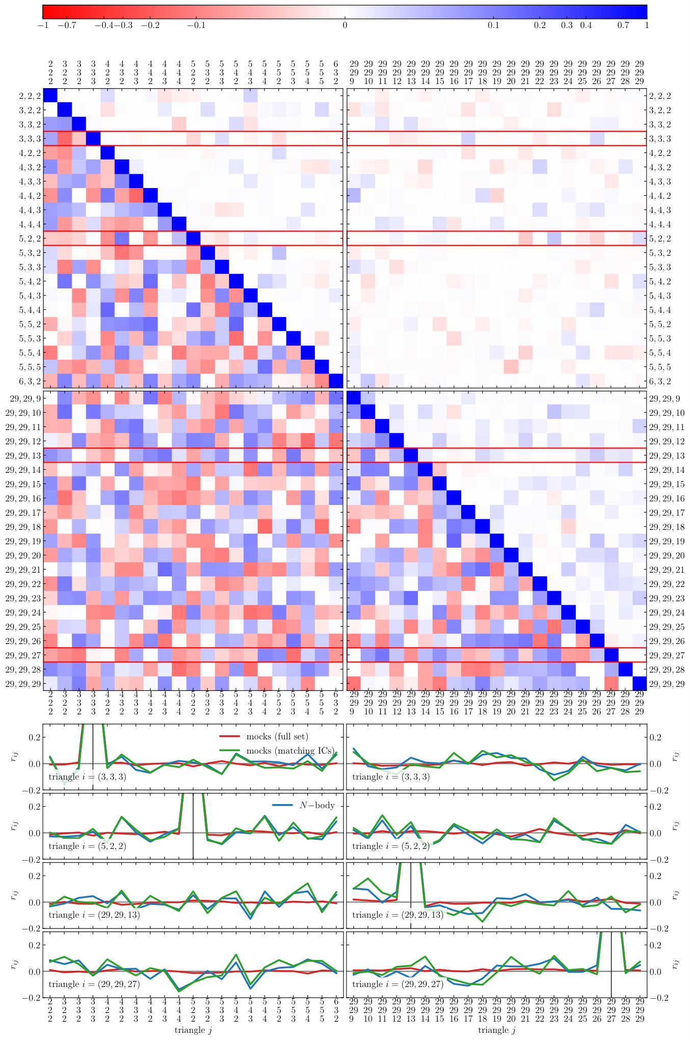
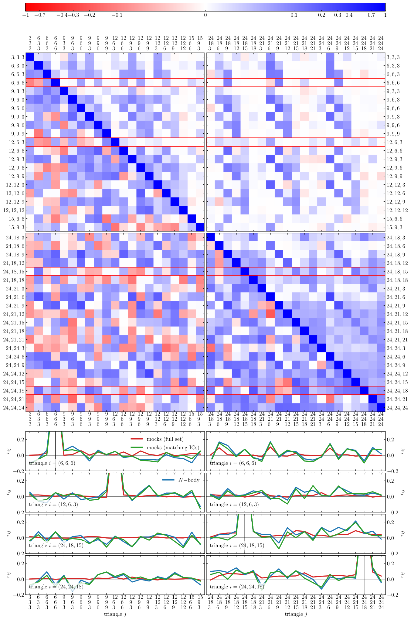
It would be misleading, based on this simple inspection, to conclude that off-diagonal contributions to the covariance matrix of the bispectrum can be safely ignored. A counterexample is shown in figure 6 where we consider bins with $s=3$. Here the top panels show again the four corners of the covariance matrix up to the same maximum wavenumber, with the last triangles being $\{8,8,8\}\Delta k=\{24,24,24\}k_{f}=\{0.1,0.1,0.1\}\,h\,{\rm Mpc}^{-1}$. Several off-diagonal elements of the matrix $r_{ij}$ assume values of 10-20%. They correspond to different triangles that share one or more sides and it is expected that the bispectrum covariance receives contributions from the non-Gaussian terms in this case. These features are present as well in the covariance estimated from the 298 simulations, but the noise affecting them is also of the order of 10-20%. Correlations among different triangles are present for any binning scheme and in the same overall amount.

In order to quantify the importance of off-diagonal terms, let us consider the cumulative signal-to-noise ratio for the bispectrum defined as

$$\left(\frac{S}{N}\right)^{2}=\sum^{N_{\rm t}(k_{\rm max})}_{i,j}B_{i}\,C_{ij}^{-1}\,B_{j}\,,$$

(2.12)

where the indices $i$ and $j$ run over all triangle configurations having no sides larger than $k_{\rm max}$.

It is interesting to see how this quantity changes if one neglects the contribution from off-diagonal terms in the covariance. This test is performed in the left-hand-side panel of figure 7 where we use the “signal” and the “noise” extracted from the 10,000 mocks. In this case we can expect a sufficiently precise determination of the covariance matrix (and its inverse), with a residual statistical error on the order of a few percent. Here the solid and dashed lines represent, respectively, the results using the full covariance and the diagonal part alone. Note that off-diagonal terms become increasingly more important as $k_{\rm max}$ grows, causing a reduction of $(S/N)^{2}$ by a factor of two at $k_{\rm max}\sim 0.08\,h\,{\rm Mpc}^{-1}$. In the right-hand-side panel, instead, we repeat the test by using the bispectrum measurements $B_{i}$ and their variance $\Delta B_{i}$ from the N-body simulations. In this case, the covariance matrix is obtained using the relation $C_{ij}=\Delta B_{i}\,\Delta B_{j}\,r_{ij}$ where the cross-correlation matrix is estimated from the 10,000 mocks. The results are essentially the same as in the left-hand-side panel.

The comparison between mocks and simulations over the subset of realisations sharing the initial seeds performed in terms of the bispectrum variance, figure 4, as well as in terms of cross-correlation coefficients $r_{ij}$, constitutes our main justification for using the covariance from the larger set of 10,000 Pinocchio runs in the analysis of the simulation measurements. In what follows, we will assume that any systematic error in the determination of the bispectrum covariance matrix based on the approximate halo mocks is negligible, but we will comment on those few instances where a small residual systematic error could affect our results.

We use a theoretical model for the halo bispectrum that only includes leading-order contributions in standard perturbation theory (SPT, see [42] for a review). This choice is motivated by the fact that we consider only large-scale measurements, with wavevectors $k<k_{\rm max}=0.12\,h\,{\rm Mpc}^{-1}$ at redshift $z=1$. Specifically, we consider the expression

	$\displaystyle B_{h}(\mathbf{k}_{1},\mathbf{k}_{2},\mathbf{k}_{3})$	$\displaystyle=$	$\displaystyle b_{1}^{3}\,B_{\mathrm{TL}}(\mathbf{k}_{1},\mathbf{k}_{2},\mathbf{k}_{3})+b_{2}b_{1}^{2}\,\Sigma(\mathbf{k}_{1},\mathbf{k}_{2},\mathbf{k}_{3})+2\gamma_{2}b_{1}^{2}\,K(\mathbf{k}_{1},\mathbf{k}_{2},\mathbf{k}_{3})+$		(3.1)
			$\displaystyle+\frac{1}{(2\pi)^{3}\bar{n}}(1+\alpha_{1})\,b_{1}^{2}\,\left[P_{\mathrm{L}}(k_{1})+P_{\mathrm{L}}(k_{2})+P_{\mathrm{L}}(k_{3})\right]+\frac{1}{(2\pi)^{6}\bar{n}^{2}}(1+\alpha_{2})\;,$

that derives from assuming a second-order bias expansion [43, 44, 45] with parameters $b_{1}$ (linear bias), $b_{2}$ (quadratic bias) and $\gamma_{2}$ (tidal bias, for which we use the notation in [44, 46]) as well as possible corrections to Poissonian shot noise [47, 48, 49, 50] quantified by the coefficients $\alpha_{1}$ and $\alpha_{2}$. Consistent with the leading-order approximation, we ignore any scale-dependence of these shot-noise/stochastic parameters [50, 46]. In eq. (3.1),

$$B_{\mathrm{TL}}(\mathbf{k}_{1},\mathbf{k}_{2},\mathbf{k}_{3})=2F_{2}(\mathbf{k}_{1},\mathbf{k}_{2})P_{\mathrm{L}}(k_{1})P_{\mathrm{L}}(k_{2})+2~\mathrm{perm.}\,,$$

(3.2)

denotes the tree-level SPT solution for the matter bispectrum, where

$$F_{2}(\mathbf{k}_{1},\mathbf{k}_{2})=\frac{5}{7}+\frac{1}{2}\frac{\mathbf{k}_{1}\cdot\mathbf{k}_{2}}{k_{1}\,k_{2}}\left(\frac{k_{1}}{k_{2}}+\frac{k_{2}}{k_{1}}\right)+\frac{2}{7}\left(\frac{\mathbf{k}_{1}\cdot\mathbf{k}_{2}}{k_{1}\,k_{2}}\right)^{2}$$

(3.3)

is the usual second-order kernel and $P_{\mathrm{L}}(k)$ is the linear power spectrum for the perturbations in the matter density. Similarly,

$$\Sigma(\mathbf{k}_{1},\mathbf{k}_{2},\mathbf{k}_{3})=P_{\mathrm{L}}(k_{1})P_{\mathrm{L}}(k_{2})+2~\mathrm{perm.}\;,$$

(3.4)

and

$$K(\mathbf{k}_{1},\mathbf{k}_{2},\mathbf{k}_{3})=\left[\left(\hat{\mathbf{k}}_{1}\cdot\hat{\mathbf{k}}_{2}\right)^{2}-1\right]P_{\mathrm{L}}(k_{1})P_{\mathrm{L}}(k_{2})+2~\mathrm{perm.}\;.$$

(3.5)

Finally, it is worth noticing that, in alternative perturbative approaches [51], additional terms appear in the tree-level bispectrum of biased tracers [52, 53, 54]. However, as they present a $k^{2}$ scaling similar to 1-loop corrections in SPT we neglect them in this work.

We fix the cosmological parameters to the actual values of the N-body simulations and only fit the five bias plus shot-noise parameters. This allows us to pre-compute the functions $P_{\mathrm{L}},B_{\mathrm{TL}},\Sigma$ and $K$, as well as the fully averaged sum of the three linear power spectra in eq. (3.1), and thus minimize the time required to evaluate the model and the likelihood function. Note that, since we fit the model to measurements of the bispectrum from individual simulations, we use the halo number density $\bar{n}$ measured in each box to evaluate the Poissonian shot-noise contribution.

Although eq. (3.1) contains five tunable parameters, it is important to assess how many of them can be justified by the data as a function of $k_{\rm max}$. For this reason, we consider different models obtained by reducing the parameter space in eq. (3.1) as follows (see also table 2 for a compact summary):

• •

  ${\mathcal{M}}_{1}$: The most basic model assumes a linear-bias relation ($b_{2}=\gamma_{2}=0$) and Poissonian shot noise ($\alpha_{1}=\alpha_{2}=0$);

• •

  ${\mathcal{M}}_{1f}$: This is still a 1-parameter model where both quadratic parameters $b_{2}$ and $\gamma_{2}$,⁵⁵ 5 The definition of the tidal-bias operator adopted in [55] differs from ours. They use the “square” of the traceless tidal field to define it while we use the second-order Galileon operator. As a result, our second-order bias, $b_{2}$, relates to theirs, $\tilde{b}_{2}$, as $b_{2}=\tilde{b}_{2}+\frac{4}{3}\gamma_{2}$. are expressed as functions of the linear bias parameter, respectively through the fitting function $\tilde{b}_{2}(b_{1})=0.412-2.143\,b_{1}+0.929\,b_{1}^{2}+0.008\,b_{1}^{3}$ provided by [55] (see also [56, 57]) and assuming local Lagrangian biasing⁶⁶ 6 Several recent studies provide evidence of small systematic deviations from this relation, with $\gamma_{2}$ being slightly more negative but still linearly related to $b_{1}$ [58, 59, 60]. Larger deviations have been measured by [61] [62], i.e. $\gamma_{2}=-\frac{2}{7}(b_{1}-1)$ [44, 45]. For the shot-noise corrections we assume the Poisson prediction $\alpha_{1}=\alpha_{2}=0$;

• •

  ${\mathcal{M}}_{2b_{2}}$: 2-parameter model with $b_{1}$ and $b_{2}$ free to vary while $\gamma_{2}=-\frac{2}{7}(b_{1}-1)$ and $\alpha_{1}=\alpha_{2}=0$;

• •

  ${\mathcal{M}}_{2\gamma_{2}}$: 2-parameter model with $b_{1}$ and $\gamma_{2}$ free to vary while $\tilde{b}_{2}(b_{1})$ follows the fit in [55] and $\alpha_{1}=\alpha_{2}=0$;

• •

  ${\mathcal{M}}_{2\mathrm{loc}}$: 2-parameter, local model with $b_{1}$ and $b_{2}$ free to vary while $\gamma_{2}=0$ and $\alpha_{1}=\alpha_{2}=0$.

• •

  ${\mathcal{M}}_{3}$: 3-parameter model with all bias parameters free to vary while $\alpha_{1}=\alpha_{2}=0$; this is used as reference model;

• •

  ${\mathcal{M}}_{4}$: 4-parameter model with additional freedom in the description of shot noise; a single shot-noise correction parameter $\alpha_{1}=\alpha_{2}$ is allowed to vary, as assumed for instance in [14, 16], in addition to the three bias parameters;

• •

  ${\mathcal{M}}_{5}$: 5-parameter model where all parameters in eq. (3.1) are free to vary.

It is worth stressing that our main goal here is to assess the constraining power of the halo bispectrum as a function of $k_{\rm max}$ without considering other data that set additional constraints and break degeneracies among the model parameters. We will discuss the combination with the halo power spectrum in our future work. Note that forthcoming galaxy redshift surveys will span much smaller volumes than our N-body simulations but also deal with a substantially higher number-density of tracers ($\gtrsim 10^{-3}h^{3}$ Mpc^-3). A redshift bin of size $\Delta z=0.2$, that is large enough to properly measure BAO features along the line of sight, corresponds to a volume at most of about 10-12$\,h^{-3}\,{\rm Gpc}^{3}$ both for DESI [31] or Euclid [63]. Therefore, our bispectrum measurements are subject to a smaller sample variance and larger shot-noise corrections with respect to what will be available from future galaxy samples.

In practice, the bispectrum is estimated by averaging over a number of triangle configurations (see section 2.2). It is therefore imperative that the theoretical predictions are treated in the same way. Since our measurements are performed in periodic boxes, the average over the bin is in fact a sum over fundamental triangles:

$$B_{\mathrm{bin}}(k_{1},k_{2},k_{3})=\frac{1}{N_{B}(k_{1},k_{2},k_{3})}\sum_{\mathbf{q}_{1}\in k_{1}}\sum_{\mathbf{q}_{2}\in k_{2}}\sum_{\mathbf{q}_{3}\in k_{3}}\delta_{K}(\mathbf{q}_{123})B_{h}(\mathbf{q}_{1},\mathbf{q}_{2},\mathbf{q}_{3})\;.$$

(3.6)

For the tree-level model introduced in eq. (3.1), this operation can be performed exactly in a relatively short time (see also [13]). However, in general, this is a non-trivial problem. If the prediction for a single configuration includes loop corrections, it becomes prohibitively expensive to evaluate the average (although, in certain perturbative schemes, it should be possible to approximately replace the sum with an integral). We explore here the impact of a pragmatic solution that minimizes the number of evaluations of the function $B_{h}$. The idea is to replace the bin average with the bispectrum evaluated at a single “effective” triangle configuration defined in terms of the triangle bin $\{k_{1}$, $k_{2}$, $k_{3}\}$ and the bin size $\Delta k$. Generalizing [64] to discrete Fourier transforms, a simple choice would be

$$\widetilde{k}_{i}(k_{1};k_{2},k_{3})=\frac{1}{N_{B}(k_{1},k_{2},k_{3})}\sum_{\mathbf{q}_{1}\in k_{1}}\sum_{\mathbf{q}_{2}\in k_{2}}\sum_{\mathbf{q}_{3}\in k_{3}}q_{i}\,\delta_{K}(\mathbf{q}_{123})\;.$$

(3.7)

Notice that, with this definition, an “equilateral bin” with $k_{1}=k_{2}=k_{3}$ would correspond to an equilateral “effective” configuration with $\widetilde{k}_{1}=\widetilde{k}_{2}=\widetilde{k}_{3}$. However, most of the fundamental triangles $\{\mathbf{q}_{1},\mathbf{q}_{2},\mathbf{q}_{3}\}$ contributing to such a bin are not equilateral. We take this into account by introducing a second effective configuration in which we sort the sidelengths of the fundamental triangles before averaging them (see also [13]). For instance, the largest effective side would be given by

$$\widetilde{k}_{l}(k_{1},k_{2},k_{3})=\frac{1}{N_{B}(k_{1},k_{2},k_{3})}\sum_{\mathbf{q}_{1}\in k_{1}}\sum_{\mathbf{q}_{2}\in k_{2}}\sum_{\mathbf{q}_{3}\in k_{3}}\max(q_{1},q_{2},q_{3})\,\delta_{K}(\mathbf{q}_{123})\,,$$

(3.8)

and similar definitions can be written for the middle and smallest values $\widetilde{k}_{m}$ and $\widetilde{k}_{s}$.

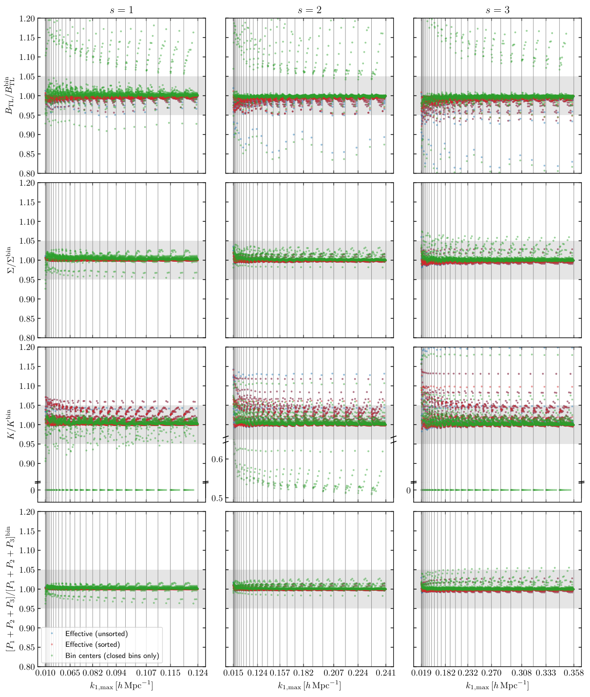
In figure 8, we show how much the bispectrum evaluated at the effective configurations differs from the correct bin average given in eq. (3.6). We plot all the different contributions to the tree-level bispectrum separately. For $s=1$, discrepancies are generally at the few percent level, with a small subset of configurations exceeding 5% only for the $K$ term. As expected, such differences grow with the bin size but remain smaller than 5%, now with the exception of $K$ and the matter contribution $B_{\rm TL}$, i.e. both shape-dependent terms. For the specific case of squeezed isosceles triangles (i.e. those configurations with bin centers given by $k_{1}=k_{2}$ and $k_{3}=\Delta k$) we notice that using the averages of the sorted wavenumbers as in eq. (3.8) works much better than the other case. For completeness, in figure 8, we also consider theoretical predictions for the bispectrum directly evaluated at the bin centers $\{k_{1},k_{2},k_{3}\}$, clearly limited to those triangle bins whose triplet centers form a closed triangle (“closed bins”). In general, using the bin center performs much worse than any of the two effective solutions we introduced above, and moreover this treatment is not well defined for open bins. For instance, for collinear triangles with $k_{1}=k_{2}+k_{3}$, it always gives $K=0$ for the $s=1$ and $s=3$ cases.

The likelihood function $\mathcal{L}$ of a hypothesis given some data is proportional to the probability of obtaining the data under the assumption that the hypothesis is true. The simplest and most-commonly made assumption is to treat the data as generated by an unbiased estimator that produces Gaussian measurement errors. For a set of $N_{\mathrm{t}}$ bispectrum configurations, this gives

$$\ln\mathcal{L}=-\frac{1}{2}\sum_{i=1}^{N_{\mathrm{t}}}\sum_{j=1}^{N_{\mathrm{t}}}\delta B_{i}\,C_{ij}^{-1}\,\delta B_{j}\equiv-\frac{1}{2}\,\delta\mathbf{B}^{T}\cdot\mathbb{C}^{-1}\cdot\delta\mathbf{B}=-\frac{\chi^{2}}{2}\;,$$

(3.9)

with $\delta B_{i}=B_{i}^{\mathrm{obs}}-B^{\mathrm{th}}_{i}$ where $B_{i}^{\mathrm{obs}}$ denotes the observed (binned) bispectrum for the triangle configuration $t_{i}$ and $B^{\mathrm{th}}_{i}$ is the corresponding theoretical prediction. The second expression on the rhs adopts a compact notation expressed in terms of the bispectrum data vector $\mathbf{B}$ and the corresponding covariance matrix $\mathbb{C}$. In our analysis, however, the covariance matrix is numerically estimated from the 10,000 mocks described in section 2.3 using their sample covariance. Despite the large number of realisations, the resulting estimate, $\tilde{\mathbb{C}}$ is still plagued by statistical errors that generate two effects. First, on average, they produce a bias in the precision matrix [65]. Secondly, they lead to a loss of information in the parameter-inference process (i.e. the resulting posterior probability distributions of the model parameters are, on average, broader than in the absence of noise) [66, 67, 68, 69, 70]. It has been shown that considering Gaussian errors and marginalizing over the (unknown) population covariance matrix (by assuming an independence Jeffreys prior) given the noisy estimate leads to the non-Gaussian likelihood [25]:

$$\ln\mathcal{L}=-\frac{N_{M}}{2}\ln{\left[1+\frac{\delta{\mathbf{B}}\cdot{\widetilde{\mathbb{C}}}^{-1}\cdot\delta{\mathbf{B}}}{N_{M}-1}\right]}+\ln{\left(\frac{\bar{c}_{p}}{\sqrt{\det{\widetilde{\mathbb{C}}}}}\right)},$$

(3.10)

where $N_{M}$ denotes the number of simulations used to estimate the covariance matrix and $\bar{c}_{p}$ is a normalization constant that does not depend on the model parameters and we can neglect. This can be interpreted as a generalisation of the multivariate $t$-distribution. Note that eq. (3.10) has the same numerical complexity as the multivariate Gaussian in eq. (3.9) and can thus be easily used to run MCMC simulations. This is our reference method. Another approach frequently used in the literature is to adopt a Gaussian likelihood with an unbiased estimator of the precision matrix obtained by rescaling the inverse of the sample covariance matrix [65, 71]:

$$\hat{\mathbb{C}}^{-1}=\frac{N_{M}-N_{\rm t}-2}{N_{M}-1}\,\widetilde{\mathbb{C}}^{-1}\;.$$

(3.11)

We also consider this possibility. In our case, $N_{M}=10,000$ and $N_{\mathrm{t}}$ varies with the binning strategy. For $s=1$ and $k_{\rm max}\simeq 0.12\,h\,{\rm Mpc}^{-1}$, we have $N_{\mathrm{t}}\sim 2,700$ and the correction is of the order of 27% and thus not negligible. For $s=2$ and 3 and the same $k_{\rm max}$, instead, it amounts to a few percent or less. Note that the credibility intervals of the model parameters obtained using either eq. (3.10) or a Gaussian likelihood with the rescaled precision matrix given in eq. (3.11) need to be corrected in order to account for the loss of information due to the uncertainty in the covariance matrix, see e.g. [69, 70]. We will revisit this procedure in Section 5.

A related issue is assessing to what degree eq. (3.9) provides a good approximation to the actual likelihood function. Departures from the ideal case could originate for different reasons. In the first place, we can expect that bispectrum estimates at the largest scales have a non-Gaussian probability distribution simply because they behave like the third power of the Gaussian field $\delta_{h}(\mathbf{q})$ [19, 72]. In fact, while at small scales these measurements get contributions from a large number of Fourier modes and Gaussianity is recovered due to the central limit theorem, for $k$-bins close to the fundamental wavenumber $k_{f}$, only a few modes contribute, and a certain degree of non-Gaussianity could be present. In addition, one can expect a non-Gaussian distribution to arise from the small-scale non-linear evolution and non-linear bias. However, after inspecting the noisy probability density function of our 298 bispectrum measurements, as well as the values of skewness and kurtosis of the distributions of each individual triangle configuration normalised by their standard errors, we could not detect any significant departure from a Gaussian distribution at the scales that are relevant for this work.

Our ultimate goal is to assess the suitability of different theoretical models for the halo bispectrum on large scales. We thus fit the models to the measurements extracted from our $N_{R}=298$ N-body simulations. Since the different realisations are statistically independent, we write the total likelihood function as the product of the likelihoods of the individual measurements or, equivalently,

$$\ln\mathcal{L}_{\mathrm{\rm tot}}=\sum_{\alpha=1}^{N_{R}}\ln\mathcal{L}_{\alpha}\;.$$

(3.12)

For the partial likelihood functions, we use eq. (3.10), neglecting the normalisation constant, as our benchmark method. For comparison, we also use eq. (3.9) combined with eq. (3.11). Note that, in the Gaussian case, this procedure gives the same parameter constraints as fitting the mean of our measurements with a suitably rescaled covariance matrix (e.g. [22]). This does not hold true in general, though.

We assume uniform priors for all the model parameters (see Table 3). More specifically, for the shot-noise parameters, we consider two possibilities. We first consider non-informative, very broad priors that do not influence the inference process (so that it is fully determined by the bispectrum data). In the second set of priors for the shot noise parameters, we force the shot noise to be positive (i.e. $\alpha_{1,2}>-1$) and make sure that corrections are not larger than the Poisson terms.

We evaluate the posterior distribution by means of Monte Carlo Markov Chain simulations using the Python affine-invariant sampler emcee [73]. For each run, we use 100 walkers to sample the parameter space. To make sure that they are sufficiently converged, we stop the simulations after 50 integrated autocorrelation times [74].

We consider a set of candidate models $\mathcal{M}_{k}\in\mathscr{M}$ for the halo bispectrum (each characterized by the parameters set $\boldsymbol{\theta}_{k}$) and use different criteria to select which of them “better” agrees with the measurements from our simulations. Two major threads run through the statistical literature on Bayesian model selection that go under the names of “explanatory” and “predictive” modelling. Let us consider a particular phenomenon or mechanism that gives rise to noisy data (the Data Generating Process or DGP). A model is an often imperfect collection of mathematical and statistical rules giving rise to an output that resembles the actual data in important ways. Explanatory modelling tests theoretically motivated hypotheses and looks for the “true model” (i.e. the DGP or approximations thereof) by examining posterior probabilities given the observed data [75]. Predictive modelling, on the other hand, searches for the model that makes the best prediction of future observations generated by the same DGP as the observed data. This is based on the posterior predictive probability distribution function which gives the probability of future measurements conditional on the observed data:

$$p(\mathrm{new\ data}|\mathrm{data},\mathcal{M}_{k})=\int p(\mathrm{new\ data}|\boldsymbol{\theta}_{k},\mathcal{M}_{k})\,P(\boldsymbol{\theta}_{k}|\mathrm{data})\,\mathrm{d}\boldsymbol{\theta}_{k}\;,$$

(4.1)

where $P$ denotes the posterior distribution of $\boldsymbol{\theta}_{k}$ given the data. For finite and noisy measurements, the two concepts possibly lead to different conclusions. In this work, we make use of one model selection criterion from each class.

We would like to assess which models provide a good fit to the data and which do not. In classical statistics, the maximum-likelihood method is often used to determine the best-fit model parameters $\hat{\boldsymbol{\theta}}$ for a given dataset. A test statistic (e.g. the $\chi^{2}$) is then selected to determine the “significance” of the fit [87]. Under the null hypothesis that the data are actually sampled from the model with $\hat{\boldsymbol{\theta}}$, one computes the conditional frequentist probability of obtaining as many or more extreme data of the test statistic. This $p$-value corresponds to the long-run frequency taken over the sampling distribution of the data under the null hypothesis (i.e. it is the probability that other unobserved data-sets would be more extreme than the one that was observed in terms of the test statistic). When the $p$-value for an experiment is small, then one has to assume that either an unusual event has occurred or that the null hypothesis is not true. Thus, the smaller the $p$ value, the less it is plausible that the null hypothesis is true.

Concern about the interpretation of $p$-values is widespread in statistics. Well-known problems of this approach are (i) that it is not possible to consider nuisance parameters and (ii) that it depends on how the data acquisition process is terminated and thus violates the likelihood principle.

Several authors have developed a Bayesian motivated adaptation of the classical goodness-of-fit test based on the $p$-value [88, 89, 90, 82]. The method relies on the posterior predictive probability distribution function given in equation (4.1). This function gives the probability (conditional on the observed data) of replicated data that could have been observed or, to think in predictive terms, that would be observed in the future if the experiment is repeated. Note that what is kept fixed here is the observed data while the classical method relies on probabilities that are conditional on the parameters of the best-fit model $\hat{\boldsymbol{\theta}}$ (i.e. the set $\hat{\boldsymbol{\theta}}$ is kept fixed). The argument then proceeds as follows. A discrepancy variable $\Delta(\mathrm{data},\boldsymbol{\theta})$ is introduced to quantify the deviation of the model (with parameters $\boldsymbol{\theta}$) from the data. The posterior predictive $p$-value (ppp) of $\Delta$ is defined as

$$\mathrm{ppp}=\mathrm{Prob}\left[\Delta(\mathrm{replicated\ data},\boldsymbol{\theta})\geq\Delta(\mathrm{data},\boldsymbol{\theta})|\mathrm{data}\right]\;,$$

(4.6)

where the probability is taken over the joint distribution

$$P(\boldsymbol{\theta},\mathrm{replicated\ data}|\mathrm{data})=p(\mathrm{replicated\ data}|\boldsymbol{\theta})\,P(\boldsymbol{\theta}|\mathrm{data})\;.$$

(4.7)

In practice, we compute the ppp of $\Delta$ using MCMC simulations by drawing one replica from the statistical model for each step of the chain. The estimated ppp corresponds then to the fraction of steps for which the discrepancy variable equals or exceeds its realised value. A ppp which is close to zero or one indicates that the realised data have a low probability of occurring under the postulated model, i.e. that the model does not fit the data well. It is important to stress, however, that ppp’s do not have in general a uniform distribution under the true model (meaning that the probability to find ppp $>0.95$ is not necessarily 5 percent) as they often tend to have distributions that are more concentrated around 0.5. Therefore, if one wants to associate a precise statistical significance to them, they need to be calibrated.

In this work, we use the ppp as a measure of goodness of fit by adopting the log likelihood as the discrepancy variable. We perform the calibration of the ppp’s by generating artificial data based on our reference model with added noise and by fitting them. We find that the distribution of our ppp’s is remarkably close to uniform under the true model. Therefore, in the analysis of the N-body data, we interpret extreme values of ppp near zero or one as revealing a systematic misfit between the bispectrum measurements and the model predictions that cannot be ignored. However, in order to facilitate understanding to readers who are more familiar with frequentist goodness-of-fit tests, we also provide the value of the posterior averaged $\chi^{2}$ statistic and the corresponding upper one-sided 95 per cent confidence limit as a function of $k_{\rm max}$ (see Section 5.1 for further details). Note that the number of degrees of freedom that should be associated to this statistic is the total number of data points (as taking the posterior average gives a larger value than minimizing the $\chi^{2}$ as in equation (4.5) for the deviance).

Finally, in order to quantify the degree to which a model systematically deviates from the actual measurements at the level of single data points, we make use of a technique known as graphical posterior predictive checking [88, 90]. In line with the ppp, this concept adopts a frequentist-like approach in a fully Bayesian framework. The underlying idea is that, if a model provides a good fit, it could be used to generate replicated data that look like those that have been observed. In practice, we compute the difference between each realised data point (i.e. the measurements from the N-body simulations) and the mean of the replicated data sampled from the posterior probability distribution function (i.e. by considering one replica for each model sampled by the Markov chain). We then convert this difference into a standardized residual, $R$, by expressing it in units of the rms uncertainty of the data. Systematic deviations with $|R|\gg 1$ indicate potential shortcomings of the model.

As a starting point, we fit model $\mathcal{M}_{3}$ to our set of bispectrum measurements using the likelihood function given in eq. (3.10). Bin averages for the model predictions are evaluated exactly using eq. (3.6). We refer to this combination of choices as our reference study.

Figure 9, like many others that follow, displays our results in five complementary panels. In the top-left corner, we show the mean and the rms values of the posterior distribution⁸⁸ 8 We do not correct the width of the posteriors for the loss of information due to the uncertainty in the covariance matrix [69]. In fact, this is impossible to do in an exact way [70]. Moreover, for all scales at which we obtain a good fit, the expected size of the correction (a few percent) is several times smaller than the statistical uncertainty with which we measure the rms value of the model parameters in the MCMC simulations. for each model parameter as a function of $k_{\rm max}$. The goodness of fit is displayed in the top-right panel. Here, we show the ppp⁹⁹ 9 Replicated data are generated by adding Gaussian noise (with covariance matrix ${\widetilde{\mathbb{C}}}$) to the theoretical models at each step of the MCMC simulations, meaning that the quantity $\delta{\mathbf{B}}_{\mathrm{repl}}\cdot{\widetilde{\mathbb{C}}}^{-1}\cdot\delta{\mathbf{B}}_{\mathrm{repl}}$ follows a $\chi^{2}$ distribution with $N_{\mathrm{t}}$ degrees of freedom for each realisation. and the posterior-averaged $\chi^{2}$ statistic divided by the number of data points, both as a function of $k_{\rm max}$. The central panel presents contour plots for the joint posterior density of all parameter pairs at $k_{\rm max}=0.082\,h\,{\rm Mpc}^{-1}$. This particular value has been selected for two reasons: i) it is an exact multiple of all the bin sizes we consider, thus ensuring that all measurements contain the same information; ii) it approximately coincides with the largest $k_{\rm max}$ for which the fits we present are good. Finally, in the bottom panel, we provide a direct comparison of the data and the fit (at $k_{\rm max}=0.082\,h\,{\rm Mpc}^{-1}$) in terms of the standardized residuals of the posterior predictive checks (PPCs) described at the end of section 4.2. In practice, we compute the difference between the measured bispectrum and the posterior mean of the replicas. The result is then averaged over all the realizations and normalized to the standard deviation of the measurements. Equilateral (binned) configurations are highlighted with vertical lines, so that from one vertical line to the other we span all configuration shapes with $k_{1}\geq k_{2}\geq k_{3}$ at fixed $k_{1}$.

In order to test the reliability of the fits presented above, we also derive the linear-bias parameter by directly comparing the halo-matter cross power spectrum and the matter power spectrum of the N-body simulations at very large scales. We find a value of $b_{1}^{\times}=2.7133\pm 0.0007$, where the superscript here indicates that this measurement comes from cross-correlating halos and matter. In figure 9, this result is represented as a narrow horizontal band in the top-left panel and as a vertical band in the center-right panel, both painted gray.

Coming to the specific results of our benchmark study, we note that the range of validity of model $\mathcal{M}_{3}$ does not extend beyond $k_{\rm max}=0.1\,h\,{\rm Mpc}^{-1}$ and shows some dependence on the bin size. The ppp approaches one at $k_{\rm max}$ of, approximately, $0.082,0.107$ and $0.119\,h\,{\rm Mpc}^{-1}$ for $\Delta k=k_{f},2k_{f}$ and $3k_{f}$, respectively. Similar conclusions can be drawn based on $\langle\chi^{2}\rangle_{\mathrm{post}}$. The values of $k_{\rm max}$ for which a good fit is achieved also correspond to consistent posterior probability distributions for the model parameters. All fits provide compatible results (within the statistical uncertainty) up to $k_{\rm max}\sim 0.08\,h\,{\rm Mpc}^{-1}$. When we include smaller scales in the analysis, instead, the location of the posterior for $\gamma_{2}$ starts running with $k_{\rm max}$ and we simultaneously obtain unsatisfactory values of the goodness-of-fit statistics. The posterior probabilities for $k_{\rm max}=0.082\,h\,{\rm Mpc}^{-1}$ show marked degeneracies between the model parameters that cannot be individually constrained apart from $b_{1}$. The standardized residuals of the PPCs do not single out any particular triangle configuration for which the model systematically deviates from the data for any binning scheme. Note that the goodness of fit at large $k_{\rm max}$ could deteriorate either because the tree-level models become inaccurate on small scales but also because our estimate of the covariance matrix becomes more and more imprecise.

The relatively small difference among the results for different bin sizes are to some extent expected. In general, the ability of the bispectrum to break degeneracies between parameters depend on the different dependence on shape of the different contributions. This is clearly affected by the binning. In particular, it is reduced by a larger binning. At the same time, a larger binning also implies smaller error bars. The combination of such different factors is likely at the origin of the observed differences.

We now fit models ${\mathcal{M}}_{4}$ and ${\mathcal{M}}_{5}$ to the bispectrum data. They extend model ${\mathcal{M}}_{3}$ to include corrections to Poissonian shot noise that are routinely included in the analysis of survey data, e.g. [16, 91]. Figure 10 compares the results for the three models for the measurements with $s=1$ when using broad priors for the shot-noise parameters. Analogous results are obtained adopting one of the other binning schemes. The most important thing to notice is that adding extra shot-noise parameters does not lead to any significant improvement in the goodness of fit and thus does not extend the range of validity of the models in terms of $k_{\rm max}$. Further insight is obtained by looking at the PPCs for $k_{\rm max}=0.082\,h\,{\rm Mpc}^{-1}$ (not shown): the residuals are virtually identical for the three models. In general, the fit results for ${\mathcal{M}}_{4}$ are very similar to ${\mathcal{M}}_{3}$ as, for sufficiently large $k_{\rm max}$, the additional parameter is always well constrained to be close to zero. On the other hand, large degeneracies between $\alpha_{1}$ and $\alpha_{2}$ (that, in this case, can assume opposite signs) as well as between the shot-noise and the bias parameters are present for ${\mathcal{M}}_{5}$. This leads to substantially larger marginalised posteriors for the bias parameters. It is also worth stressing that the loose constraints set by the data on $\alpha_{1}$ and $\alpha_{2}$ span a much larger range than expected from theoretical shot-noise models [92, 50]. We thus conclude that the large-scale bispectrum is insufficient to inform these models.

Figure 11 shows a comparison similar to the one shown in figure 10, but for the narrower priors on the shot-noise parameters. As in the previous case, both for $\mathcal{M}_{4}$ and $\mathcal{M}_{5}$, $\alpha_{1}$ is well constrained and consistent with 0, while in $\mathcal{M}_{5}$, $\alpha_{2}$ is completely unconstrained. On the other hand, the results for the bias parameters are essentially unaffected by the introduction of shot-noise parameters with such priors.

In figure 12, we apply model-selection techniques to the nested models $\mathcal{M}_{3}$, $\mathcal{M}_{4}$, and $\mathcal{M}_{5}$ considering both priors sets. We first look at the constraining power of our bispectrum data with $s=1$ (similar results are found for the other bin sizes). The top-right and middle-right panels show the effective number of parameters of the fits as a function of $k_{\rm max}$, respectively for the broad and narrow shot-noise priors. While all parameters of $\mathcal{M}_{3}$ and $\mathcal{M}_{4}$ stop being prior dominated for $k_{\rm max}\simeq 0.04\,h\,{\rm Mpc}^{-1}$, the bispectrum data can fully constrain $\mathcal{M}_{5}$ only from $k_{\rm max}\simeq 0.06\,h\,{\rm Mpc}^{-1}$ for the broad priors, and from $k_{\rm max}\simeq 0.08\,h\,{\rm Mpc}^{-1}$ for the narrow priors. In the top-left and middle-left panels, instead, we show the DIC difference with respect to $\mathcal{M}_{3}$, again for broad and narrow priors respectively. In both cases, for small values of $k_{\rm max}$, $\mathcal{M}_{3}$ is slightly preferred by the DIC, although with low significance. A fair conclusion is that, for $k_{\rm max}<0.09\,h\,{\rm Mpc}^{-1}$, the three models provide very similar DIC and cannot be ranked. On smaller scales, the DIC strongly prefers $\mathcal{M}_{5}$ but this is irrelevant as none of the models provides an acceptable goodness of fit. It is, in fact, quite possible that some non-linear effects that are not included in the tree-level model are partially accounted for by the shot-noise corrections. Stronger conclusions can be drawn based on the Bayes factors evaluated using the Savage-Dickey density ratio (bottom panels). In this case, for all binning schemes, $\mathcal{M}_{3}$ is decisively preferred over $\mathcal{M}_{4}$ at $k_{\rm max}\simeq 0.09\,h\,{\rm Mpc}^{-1}$ where the ratio exceeds 100 with broad shot-noise priors, and 10 for narrow shot-noise priors (although it suddenly drops for larger values of $k_{\rm max}$ where both models fail to properly fit the data). Similarly, $\mathcal{M}_{4}$ is preferred over $\mathcal{M}_{5}$ although to a lesser degree as the BF (not shown) only reaches a maximum value of about 20 at $k_{\rm max}\simeq 0.08\,h\,{\rm Mpc}^{-1}$. The bottom line of this section is that our data provide no evidence for non-Poissonian shot-noise corrections on the scales in which the tree-level model fits well, i.e. $k_{\rm max}<0.08\,h\,{\rm Mpc}^{-1}$.

In section 3.1, we have described several possibilities for reducing the freedom of our reference theoretical model $\mathcal{M}_{3}$. We now investigate whether these restricted models provide an accurate description of the bispectrum measurements extracted from our simulations and contrast them with $\mathcal{M}_{3}$.

As a first test, in figure 13, we compare models $\mathcal{M}_{1}$ and $\mathcal{M}_{2\mathrm{loc}}$ (which correspond to truncating a local Eulerian bias expansion at first and second order, respectively) with $\mathcal{M}_{3}$ (which also includes the tidal-bias term). In terms of goodness of fit, $\mathcal{M}_{1}$ fails around $k_{\rm max}\simeq 0.05\,h\,{\rm Mpc}^{-1}$, i.e. at significantly larger scales than the other models that, on the other hand, provide almost identical values for the ppp and $\langle\chi^{2}_{\nu}\rangle$. The local models retrieve different values for the bias parameters with respect to $\mathcal{M}_{3}$ (see also [44, 45]). Without combining our results with other clustering statistics, it is impossible to say whether $\mathcal{M}_{2\rm loc}$ and $\mathcal{M}_{3}$ provide a realistic description of the data since, in terms of goodness of fit, they are practically equivalent. However, it is interesting to notice that the DIC shown in the bottom-left panel of figure 13 not only strongly disfavours $\mathcal{M}_{1}$ already at $k_{\rm max}\simeq 0.03\,h\,{\rm Mpc}^{-1}$, but also clearly indicates a preference for $\mathcal{M}_{3}$ at $k_{\rm max}\simeq 0.06\,h\,{\rm Mpc}^{-1}$. Equivalent conclusions can be drawn from the Savage-Dickey ratios (not shown in the figure for the sake of brevity).

A second series of tests is conducted in figure 14. Here, we consider the models $\mathcal{M}_{1f}$, $\mathcal{M}_{2b_{2}}$ and $\mathcal{M}_{2\gamma_{2}}$ that have been obtained by mathematically relating the bias parameters of $\mathcal{M}_{3}$. It is important to remember that the relations we use have different origins. While the function $\tilde{b}_{2}(b_{1})$ is a fit to N-body simulations [55], $\gamma_{2}(b_{1})$ embodies an assumption characterizing a class of bias models that have been already ruled out by recent studies [59, 60]. We find that all models achieve essentially the same goodness of fit as our benchmark model. On the other hand, the posterior distributions of the parameters as a function of $k_{\rm max}$ show significant differences between $\mathcal{M}_{3}$ and all cases in which the local-Lagrangian relation for $\gamma_{2}$ is adopted. Only the results obtained with $\mathcal{M}_{2\gamma_{2}}$ are largely consistent with the reference model. One can also notice how assuming the $\tilde{b}_{2}(b_{1})$ relation greatly reduces error bars with respect to what happens when assuming instead the $\gamma_{2}(b_{1})$ relation. This is probably related to the fact that $b_{1}$ and $b_{2}$ are more strongly degenerate than $b_{1}$ and $\gamma_{2}$ in the fit for the benchmark model as evidenced in the contour plots at the reference scale. Also note that, when we impose one single relation among the bias coefficients, the joint posteriors for the parameters, including the derived ones, are fully consistent with the results obtained for $\mathcal{M}_{3}$ at the reference scale. On the other hand, if both relations are imposed simultaneously, we find significant tension in the joint posteriors with respect to the benchmark model, thus suggesting that the local-Lagrangian approximation is not compatible with the $\tilde{b}_{2}(b_{1})$ fit. In fact, the DIC clearly disfavours both $\mathcal{M}_{1f}$ and $\mathcal{M}_{2b_{2}}$ while $\mathcal{M}_{2\gamma_{2}}$ and $\mathcal{M}_{3}$ are essentially equivalent up to $0.1\,h\,{\rm Mpc}^{-1}$. It is important to understand how the figure on the goodness of fit (in which all the models seem to fit the data equally well) can be reconciled with the conclusions we have drawn from the DIC. The key is to remember that we are fitting a very large number of data points, namely 247,936 at the reference scale of $k_{\rm max}=0.082\,h\,{\rm Mpc}^{-1}$. The DIC is driven by the fact that the posterior average of $-\log\mathcal{L}$ for $\mathcal{M}_{3}$ is smaller than that obtained with $\mathcal{M}_{1f}$ by nearly 18. Since this difference is substantially larger than the number of extra parameters in $\mathcal{M}_{3}$, the DIC prefers this model. On the other hand, the goodness-of-fit statistic $\langle\chi^{2}_{\nu}\rangle_{\mathrm{post}}$ essentially depends on the average log-likelihood per data point which is very similar for all models. Therefore, although all models considered in this section provide a statistically acceptable fit of the data, $\mathcal{M}_{2\gamma_{2}}$ and $\mathcal{M}_{3}$ are preferred as they better describe our ensemble of measurements on small scales and do not overfit.

References

- [1] K. S. Dawson, J.-P. Kneib, W. J. Percival, S. Alam, F. D. Albareti, S. F. Anderson et al., The SDSS-IV Extended Baryon Oscillation Spectroscopic Survey: Overview and Early Data, Astron. J. 151 (2016) 44 [1508.04473].
- [2] R. Laureijs, J. Amiaux, S. Arduini, J. . Auguères, J. Brinchmann, R. Cole et al., Euclid Definition Study Report, ArXiv: 1110.3193 (2011) [1110.3193].
- [3] M. Levi, C. Bebek, T. Beers, R. Blum, R. Cahn, D. Eisenstein et al., The DESI Experiment, a whitepaper for Snowmass 2013, ArXiv: 1308.0847 (2013) [1308.0847].
- [4] Y.-S. Song, A. Taruya and A. Oka, Cosmology with anisotropic galaxy clustering from the combination of power spectrum and bispectrum, Journal of Cosmology and Astro-Particle Physics 8 (2015) 007 [1502.03099].
- [5] M. Tellarini, A. J. Ross, G. Tasinato and D. Wands, Galaxy bispectrum, primordial non-Gaussianity and redshift space distortions, Journal of Cosmology and Astro-Particle Physics 6 (2016) 014 [1603.06814].
- [6] D. Yamauchi, S. Yokoyama and K. Takahashi, Multitracer technique for galaxy bispectrum: An application to constraints on nonlocal primordial non-Gaussianities, Phys. Rev. D 95 (2017) 063530 [1611.03590].
- [7] J. Byun, A. Eggemeier, D. Regan, D. Seery and R. E. Smith, Towards optimal cosmological parameter recovery from compressed bispectrum statistics, Mon. Not. R. Astron. Soc. 471 (2017) 1581 [1705.04392].
- [8] K. C. Chan and L. Blot, Assessment of the information content of the power spectrum and bispectrum, Phys. Rev. D 96 (2017) 023528 [1610.06585].
- [9] P. Gagrani and L. Samushia, Information Content of the Angular Multipoles of Redshift-Space Galaxy Bispectrum, Mon. Not. R. Astron. Soc. 467 (2017) 928 [1610.03488].
- [10] D. Yamauchi, S. Yokoyama and H. Tashiro, Constraining modified theories of gravity with the galaxy bispectrum, Phys. Rev. D 96 (2017) 123516 [1709.03243].
- [11] D. Gualdi, M. Manera, B. Joachimi and O. Lahav, Maximal compression of the redshift-space galaxy power spectrum and bispectrum, Mon. Not. R. Astron. Soc. 476 (2018) 4045 [1709.03600].
- [12] D. Karagiannis, A. Lazanu, M. Liguori, A. Raccanelli, N. Bartolo and L. Verde, Constraining primordial non-Gaussianity with bispectrum and power spectrum from upcoming optical and radio surveys, Mon. Not. R. Astron. Soc. 478 (2018) 1341 [1801.09280].
- [13] V. Yankelevich and C. Porciani, Cosmological information in the redshift-space bispectrum, Mon. Not. R. Astron. Soc. (2018) [1807.07076].
- [14] H. Gil-Marín, J. Noreña, L. Verde, W. J. Percival, C. Wagner, M. Manera et al., The power spectrum and bispectrum of SDSS DR11 BOSS galaxies - I. Bias and gravity, Mon. Not. R. Astron. Soc. 451 (2015) 539 [1407.5668].
- [15] H. Gil-Marín, L. Verde, J. Noreña, A. J. Cuesta, L. Samushia, W. J. Percival et al., The power spectrum and bispectrum of SDSS DR11 BOSS galaxies - II. Cosmological interpretation, Mon. Not. R. Astron. Soc. 452 (2015) 1914 [1408.0027].
- [16] H. Gil-Marín, W. J. Percival, L. Verde, J. R. Brownstein, C.-H. Chuang, F.-S. Kitaura et al., The clustering of galaxies in the SDSS-III Baryon Oscillation Spectroscopic Survey: RSD measurement from the power spectrum and bispectrum of the DR12 BOSS galaxies, Mon. Not. R. Astron. Soc. 465 (2017) 1757 [1606.00439].
- [17] D. W. Pearson and L. Samushia, A Detection of the Baryon Acoustic Oscillation Features in the SDSS BOSS DR12 Galaxy Bispectrum, ArXiv e-prints (2017) [1712.04970].
- [18] Z. Slepian, D. J. Eisenstein, J. R. Brownstein, C.-H. Chuang, H. Gil-Marín, S. Ho et al., Detection of baryon acoustic oscillation features in the large-scale three-point correlation function of SDSS BOSS DR12 CMASS galaxies, Mon. Not. R. Astron. Soc. 469 (2017) 1738 [1607.06097].
- [19] R. Scoccimarro, The bispectrum: From theory to observations, Astrophys. J. 544 (2000) 597 [astro-ph/0004086].
- [20] E. Sefusatti and R. Scoccimarro, Galaxy bias and halo-occupation numbers from large-scale clustering, Phys. Rev. D 71 (2005) 063001 [astro-ph/0412626].
- [21] E. Sefusatti, M. Crocce, S. Pueblas and R. Scoccimarro, Cosmology and the bispectrum, Phys. Rev. D 74 (2006) 023522 [arXiv: astro-ph/0604505].
- [22] E. Sefusatti, M. Crocce and V. Desjacques, The halo bispectrum in N-body simulations with non-Gaussian initial conditions, Mon. Not. R. Astron. Soc. 425 (2012) 2903 [1111.6966].
- [23] P. Monaco, T. Theuns, G. Taffoni, F. Governato, T. Quinn and J. Stadel, Predicting the Number, Spatial Distribution, and Merging History of Dark Matter Halos, Astrophys. J. 564 (2002) 8 [arXiv:astro-ph/0109322].
- [24] J. Hartlap, T. Schrabback, P. Simon and P. Schneider, The non-Gaussianity of the cosmic shear likelihood or how odd is the Chandra Deep Field South?, Astron. Astrophys. 504 (2009) 689 [0901.3269].
- [25] E. Sellentin and A. F. Heavens, Parameter inference with estimated covariance matrices, Mon. Not. R. Astron. Soc. 456 (2016) L132 [1511.05969].
- [26] J. N. Grieb, A. G. Sánchez, S. Salazar-Albornoz and C. Dalla Vecchia, Gaussian covariance matrices for anisotropic galaxy clustering measurements, Mon. Not. R. Astron. Soc. 457 (2016) 1577 [1509.04293].
- [27] V. Springel, The cosmological simulation code GADGET-2, Mon. Not. R. Astron. Soc. 364 (2005) 1105 [astro-ph/0505010].
- [28] A. G. Sánchez, E. A. Kazin, F. Beutler, C.-H. Chuang, A. J. Cuesta, D. J. Eisenstein et al., The clustering of galaxies in the SDSS-III Baryon Oscillation Spectroscopic Survey: cosmological constraints from the full shape of the clustering wedges, Mon. Not. R. Astron. Soc. 433 (2013) 1202 [1303.4396].
- [29] A. Lewis, A. Challinor and A. Lasenby, Efficient computation of cosmic microwave background anisotropies in closed friedmann-robertson-walker models, Astrophys. J. 538 (2000) 473 [astro-ph/9911177].
- [30] V. Springel, N. Yoshida and S. D. M. White, GADGET: a code for collisionless and gasdynamical cosmological simulations, New Astronomy 6 (2001) 79 [astro-ph/0003162].
- [31] DESI Collaboration, A. Aghamousa, J. Aguilar, S. Ahlen, S. Alam, L. E. Allen et al., The DESI Experiment Part I: Science,Targeting, and Survey Design, ArXiv e-prints (2016) [1611.00036].
- [32] E. Sefusatti, M. Crocce, R. Scoccimarro and H. M. P. Couchman, Accurate estimators of correlation functions in Fourier space, Mon. Not. R. Astron. Soc. 460 (2016) 3624 [1512.07295].
- [33] R. Scoccimarro, Fast estimators for redshift-space clustering, Phys. Rev. D 92 (2015) 083532 [1506.02729].
- [34] A. Schneider, R. Teyssier, D. Potter, J. Stadel, J. Onions, D. S. Reed et al., Matter power spectrum and the challenge of percent accuracy, Journal of Cosmology and Astro-Particle Physics 4 (2016) 047 [1503.05920].
- [35] P. Monaco, T. Theuns and G. Taffoni, The pinocchio algorithm: pinpointing orbit-crossing collapsed hierarchical objects in a linear density field, Mon. Not. R. Astron. Soc. 331 (2002) 587 [arXiv:astro-ph/0109323].
- [36] P. Monaco, E. Sefusatti, S. Borgani, M. Crocce, P. Fosalba, R. K. Sheth et al., An accurate tool for the fast generation of dark matter halo catalogues, Mon. Not. R. Astron. Soc. 433 (2013) 2389 [1305.1505].
- [37] E. Munari, P. Monaco, E. Sefusatti, E. Castorina, F. G. Mohammad, S. Anselmi et al., Improving fast generation of halo catalogues with higher order Lagrangian perturbation theory, Mon. Not. R. Astron. Soc. 465 (2017) 4658 [1605.04788].
- [38] M. Lippich, A. G. Sánchez, M. Colavincenzo, E. Sefusatti, P. Monaco, L. Blot et al., Comparing approximate methods for mock catalogues and covariance matrices - I. Correlation function, Mon. Not. R. Astron. Soc. 482 (2019) 1786 [1806.09477].
- [39] L. Blot, M. Crocce, E. Sefusatti, M. Lippich, A. G. Sánchez, M. Colavincenzo et al., Comparing approximate methods for mock catalogues and covariance matrices II: Power spectrum multipoles, Mon. Not. R. Astron. Soc. (2019) [1806.09497].
- [40] M. Colavincenzo, E. Sefusatti, P. Monaco, L. Blot, M. Crocce, M. Lippich et al., Comparing approximate methods for mock catalogues and covariance matrices - III: bispectrum, Mon. Not. R. Astron. Soc. 482 (2019) 4883 [1806.09499].
- [41] P. Monaco, Approximate Methods for the Generation of Dark Matter Halo Catalogs in the Age of Precision Cosmology, Galaxies 4 (2016) 53 [1605.07752].
- [42] F. Bernardeau, S. Colombi, E. Gaztañaga and R. Scoccimarro, Large-scale structure of the universe and cosmological perturbation theory, Phys. Rep. 367 (2002) 1 [astro-ph/0112551].
- [43] J. N. Fry and E. Gaztañaga, Biasing and hierarchical statistics in large-scale structure, Astrophys. J. 413 (1993) 447 [astro-ph/9302009].
- [44] K. C. Chan, R. Scoccimarro and R. K. Sheth, Gravity and large-scale nonlocal bias, Phys. Rev. D 85 (2012) 083509 [1201.3614].
- [45] T. Baldauf, U. Seljak, V. Desjacques and P. McDonald, Evidence for quadratic tidal tensor bias from the halo bispectrum, Phys. Rev. D 86 (2012) 083540 [1201.4827].
- [46] A. Eggemeier, R. Scoccimarro and R. E. Smith, Bias Loop Corrections to the Galaxy Bispectrum, arXiv e-prints (2018) arXiv:1812.03208 [1812.03208].
- [47] U. Seljak, N. Hamaus and V. Desjacques, How to Suppress the Shot Noise in Galaxy Surveys, Physical Review Letters 103 (2009) 091303 [0904.2963].
- [48] N. Hamaus, U. Seljak, V. Desjacques, R. E. Smith and T. Baldauf, Minimizing the stochasticity of halos in large-scale structure surveys, Phys. Rev. D 82 (2010) 043515 [1004.5377].
- [49] K. Paech, N. Hamaus, B. Hoyle, M. Costanzi, T. Giannantonio, S. Hagstotz et al., Cross-correlation of galaxies and galaxy clusters in the Sloan Digital Sky Survey and the importance of non-Poissonian shot noise, Mon. Not. R. Astron. Soc. 470 (2017) 2566 [1612.02018].
- [50] D. Ginzburg, V. Desjacques and K. C. Chan, Shot noise and biased tracers: A new look at the halo model, Phys. Rev. D 96 (2017) 083528 [1706.08738].
- [51] L. Senatore, Bias in the effective field theory of large scale structures, Journal of Cosmology and Astro-Particle Physics 11 (2015) 007 [1406.7843].
- [52] R. Angulo, M. Fasiello, L. Senatore and Z. Vlah, On the statistics of biased tracers in the Effective Field Theory of Large Scale Structures, Journal of Cosmology and Astro-Particle Physics 9 (2015) 029 [1503.08826].
- [53] T. Fujita, V. Mauerhofer, L. Senatore, Z. Vlah and R. Angulo, Very Massive Tracers and Higher Derivative Biases, ArXiv e-prints (2016) [1609.00717].
- [54] E. O. Nadler, A. Perko and L. Senatore, On the bispectra of very massive tracers in the Effective Field Theory of Large-Scale Structure, Journal of Cosmology and Astro-Particle Physics 2 (2018) 058 [1710.10308].
- [55] T. Lazeyras, C. Wagner, T. Baldauf and F. Schmidt, Precision measurement of the local bias of dark matter halos, Journal of Cosmology and Astro-Particle Physics 2 (2016) 018 [1511.01096].
- [56] K. Hoffmann, J. Bel and E. Gaztañaga, Comparing halo bias from abundance and clustering, Mon. Not. R. Astron. Soc. 450 (2015) 1674 [1503.00313].
- [57] K. Hoffmann, J. Bel and E. Gaztañaga, Linear and non-linear bias: predictions versus measurements, Mon. Not. R. Astron. Soc. 465 (2017) 2225 [1607.01024].
- [58] S. Saito, T. Baldauf, Z. Vlah, U. Seljak, T. Okumura and P. McDonald, Understanding higher-order nonlocal halo bias at large scales by combining the power spectrum with the bispectrum, Phys. Rev. D 90 (2014) 123522 [1405.1447].
- [59] T. Lazeyras and F. Schmidt, Beyond LIMD bias: a measurement of the complete set of third-order halo bias parameters, Journal of Cosmology and Astro-Particle Physics 9 (2018) 008 [1712.07531].
- [60] M. M. Abidi and T. Baldauf, Cubic halo bias in Eulerian and Lagrangian space, Journal of Cosmology and Astro-Particle Physics 2018 (2018) 029 [1802.07622].
- [61] C. Modi, E. Castorina and U. Seljak, Halo bias in Lagrangian space: estimators and theoretical predictions, Mon. Not. R. Astron. Soc. 472 (2017) 3959 [1612.01621].
- [62] P. Catelan, C. Porciani and M. Kamionkowski, Two ways of biasing galaxy formation, Mon. Not. R. Astron. Soc. 318 (2000) L39 [astro-ph/0005544].
- [63] Euclid Collaboration, A. Blanchard, S. Camera, C. Carbone, V. F. Cardone, S. Casas et al., Euclid preparation: VII. Forecast validation for Euclid cosmological probes, arXiv e-prints (2019) arXiv:1910.09273 [1910.09273].
- [64] E. Sefusatti, M. Crocce and V. Desjacques, The matter bispectrum in N-body simulations with non-Gaussian initial conditions, Mon. Not. R. Astron. Soc. 406 (2010) 1014 [1003.0007].
- [65] T. W. Anderson, An introduction to multivariate statistical analysis. Wiley New York, 1958.
- [66] S. Dodelson and M. D. Schneider, The effect of covariance estimator error on cosmological parameter constraints, Phys. Rev. D 88 (2013) 063537 [1304.2593].
- [67] A. N. Taylor, B. Joachimi and T. D. Kitching, Putting the precision in precision cosmology: How accurate should your data covariance matrix be?, Mon. Not. R. Astron. Soc. 432 (2013) 1928 [1212.4359].
- [68] A. Taylor and B. Joachimi, Estimating cosmological parameter covariance, Mon. Not. R. Astron. Soc. 442 (2014) 2728 [1402.6983].
- [69] W. J. Percival, A. J. Ross, A. G. Sánchez, L. Samushia, A. Burden, R. Crittenden et al., The clustering of Galaxies in the SDSS-III Baryon Oscillation Spectroscopic Survey: including covariance matrix errors, Mon. Not. R. Astron. Soc. 439 (2014) 2531 [1312.4841].
- [70] E. Sellentin and A. F. Heavens, Quantifying lost information due to covariance matrix estimation in parameter inference, Mon. Not. R. Astron. Soc. 464 (2017) 4658 [1609.00504].
- [71] J. Hartlap, P. Simon and P. Schneider, Why your model parameter confidences might be too optimistic. Unbiased estimation of the inverse covariance matrix, Astron. Astrophys. 464 (2007) 399 [astro-ph/0608064].
- [72] C. Hahn, F. Beutler, M. Sinha, A. Berlind, S. Ho and D. W. Hogg, Likelihood non-Gaussianity in large-scale structure analyses, Mon. Not. R. Astron. Soc. 485 (2019) 2956 [1803.06348].
- [73] D. Foreman-Mackey, D. W. Hogg, D. Lang and J. Goodman, emcee: The MCMC Hammer, Publications of the Astronomical Society of the Pacific 125 (2013) 306 [1202.3665].
- [74] J. Goodman and J. Weare, Ensemble samplers with affine invariance, Communications in Applied Mathematics and Computational Science, Vol. 5, No. 1, p. 65-80, 2010 5 (2010) 65.
- [75] R. E. Kass and A. E. Raftery, Bayes factors, Journal of the American Statistical Association 90 (1995) 773 [https://www.tandfonline.com/doi/pdf/10.1080/01621459.1995.10476572].
- [76] H. Jeffreys, Theory of Probability, The International series of monographs on physics. Clarendon Press, 1961.
- [77] J. M. Dickey, The weighted likelihood ratio, linear hypotheses on normal location parameters, Ann. Math. Statist. 42 (1971) 204.
- [78] R. Trotta, Applications of Bayesian model selection to cosmological parameters, Mon. Not. R. Astron. Soc. 378 (2007) 72 [astro-ph/0504022].
- [79] M. .-. . Proceedings of Conference on Foundational Questions in Statistical Inference, Aarhus, ed., The direct use of likelihood for significance testing, Department of Theoretical Statistics, Institute of Mathematics, University of Aarhus, 1974.
- [80] D. J. Spiegelhalter, N. G. Best, B. P. Carlin and A. Van Der Linde, Bayesian measures of model complexity and fit, Journal of the Royal Statistical Society Series B 64 (2002) 583.
- [81] H. Akaike, Information Theory and an Extension of the Maximum Likelihood Principle, pp. 199–213. Springer New York, New York, NY, 1998.
- [82] A. Gelman, J. B. Carlin, H. S. Stern and D. B. Rubin, Bayesian Data Analysis. Chapman and Hall/CRC, 2nd ed. ed., 2004.
- [83] M. Plummer, Penalized loss functions for Bayesian model comparison, Biostatistics 9 (2008) 523 [http://oup.prod.sis.lan/biostatistics/article-pdf/9/3/523/17742541/kxm049.pdf].
- [84] A. van der Linde, Dic in variable selection, Statistica Neerlandica 59 (2005) 45 [https://onlinelibrary.wiley.com/doi/pdf/10.1111/j.1467-9574.2005.00278.x].
- [85] A. van der Linde, A bayesian view of model complexity, Statistica Neerlandica 66 (2012) 253 [https://onlinelibrary.wiley.com/doi/pdf/10.1111/j.1467-9574.2011.00518.x].
- [86] T. Ando, Predictive bayesian model selection, American Journal of Mathematical and Management Sciences 31 (2011) 13 [https://doi.org/10.1080/01966324.2011.10737798].
- [87] R. Fisher, Statistical Methods for Research Workers, Biological monographs and manuals. Oliver and Boyd, 1925.
- [88] D. B. Rubin, Bayesianly justifiable and relevant frequency calculations for the applied statistician, Ann. Statist. 12 (1984) 1151.
- [89] X.-L. Meng, Posterior predictive -values, Ann. Statist. 22 (1994) 1142.
- [90] A. Gelman, X. Meng and H. Stern, Posterior predictive assessment of model fitness via realized discrepancies, Statistica Sinica 6 (1996) 733.
- [91] E. Castorina, N. Hand, U. Seljak, F. Beutler, C.-H. Chuang, C. Zhao et al., Redshift-weighted constraints on primordial non-Gaussianity from the clustering of the eBOSS DR14 quasars in Fourier space, Journal of Cosmology and Astro-Particle Physics 2019 (2019) 010 [1904.08859].
- [92] T. Baldauf, U. Seljak, R. E. Smith, N. Hamaus and V. Desjacques, Halo stochasticity from exclusion and nonlinear clustering, Phys. Rev. D 88 (2013) 083507 [1305.2917].
- [93] K. F. Werner and C. Porciani, Renormalisation of linear halo bias in N-body simulations, arXiv e-prints (2019) arXiv:1907.03774 [1907.03774].