A sceptical analysis of Quantized Inertia2019A sceptical analysis of Quantized Inertia–References
Abstract
We perform an analysis of the derivation of Quantized Inertia (QI) theory, formerly known with the acronym MiHsC, as presented by McCulloch 2007; McCulloch 2013. Two major flaws were found in the original derivation. We derive a discrete black-body radiation spectrum, deriving a different formulation for than the one presented in the original theory. We present a numerical result of the new solution which is compared against the original prediction.
Keywords:
dark matter – galaxies: kinematics and dynamics – cosmology: theory1 Introduction
The discrepancy between observed galaxies rotation curves and the prediction using the known laws of orbital kinematics was initially observed by Rubin et al. 1980, and it is now an accepted phenomenon.
Several theories were developed to justify such discrepancies, such as the existence of a dark matter halo (Rubin 1983), or the existence of a Modified Newtonian Dynamics, MoND (Milgrom 1983) at galactic scales.
As today, no direct evidence of dark matter was detected, though many experiments such as XENON100 (Aprile et al. 2012) and SuperCDMS (SuperCDMS Collaboration et al. 2014) are looking for signal candidates. Some models support the idea that dark matter particles could be created at LHC and efforts in this direction are in progress (Abercrombie et al. 2015; Mitsou 2015; Liu et al. 2019).
MoND models remove the necessity for dark matter candidates introducing a modified law of motion for low accelerations:
| (1) |
This approach has been criticized due to the requirement of an arbitrary parameter and because it does not predict the dynamics of galaxy clusters (Aguirre et al. 2001; Sanders 2003). A new theory, by McCulloch, proposes a solution to the discrepancies observed in the galaxies’ rotation curves. This theory, named Modification of inertia resulting from a Hubble-scale Casimir effect (MiHsC) or Quantized Inertia (QI), may give a model for the galaxies’ rotation curves (McCulloch 2012) and explain some other phenomena like the Pioneer anomaly (McCulloch 2007), the flyby anomalies McCulloch 2008, the Em-drive (McCulloch 2015), opening the way for propellant-less spacecraft propulsion (McCulloch 2018). In addition, this theory provides also an intuitive explanation for objects’ inertia (McCulloch 2013).
The main strong points of this theory, as shown by eq. 7, are the absence of arbitrary tunable parameters (being based on universal constants like the Hubble constant and the speed of light), its simple formulation and the wide range of phenomena it seems to explain. Its main weak point is the fact it assumes the existence of the Unruh radiation (Unruh 1976), which is still not experimentally measured in nature, although some recent simulations seems to confirm its existence (Hu et al. 2019).
Quantized Inertia has collected some criticisms by mainstream press (Koberlein 2017), but, as today, no critical analysis was published in a peer-reviewed journal on this subject.
In the next sections we will present our analysis of Quantized Inertia: in section 2 we will perform a brief recapitulation of the theory as presented by McCulloch 2007; McCulloch 2013, in sections 3 and 4 we will present two major flaws we found in its derivation and we propose some corrections and finally, in section 5, we will present our considerations about the validity of the whole theory.
2 Recapitulation on Quantized Inertia
Quantized Inertia states two important affirmation:
- 1.
There exists a minimum acceleration any object can ever have: (see McCulloch 2017, sect. 2). Below such a value, the object’s inertia becomes zero causing the object’s acceleration to increase to the minimum value.
- 2.
Inertia is caused by the Unruh radiation imbalance between the cosmic and the Rindler horizon (McCulloch 2013, fig.1).
The rationale behind the first point is this: according to the Unruh radiation law (Unruh 1976), every accelerating object will feel a background temperature:
| (2) |
where is the reduced Planck constant, the speed of light in vacuum, the Boltzmann constant and the object’s acceleration. It is important to notice that this temperature is very tiny: for an object acceleration of , the temperature will be , making very difficult any experimental detection.
Planck’s law states such background will emit black-body radiation with spectrum:
| (3) | ||||
| with a peak wavelength: | ||||
| (4) | ||||
where is the solution of the transcendental equation and is Planck’s constant. We would like to remark that the Planck’s law describes an unconstrained system at equilibrium. This is the case in a classic black-body radiation experiment where the radiation wavelength is much smaller than the cavity size, leading to a continuous spectrum.
However, for very low temperatures, the associated radiation wavelength may become bigger than the cosmic horizon, defined as the sphere with radius equal to the Hubble distance. We introduce so the Hubble diameter defined as:
| (5) |
where is the Hubble constant11 1 In this paper we assume , as used by McCulloch 2007, for easier results comparison with the original papers. and is the speed of light in vacuum. In this case we can not consider the spectra continuous any more, because, by principle, only the wavelengths fitting twice the Hubble diameter can ever exist:
| (6) |
The minimum acceleration arises from two phenomena: for lower accelerations, the object experiences lower Unruh background radiation due to a) the shift of the spectra behind the Hubble diameter and b) a more sparse sampling of the black body radiation spectra, as shown in fig. 1.

The consideration expressed above were used to define a Hubble Scale Casimir-like effect: using a not better specified direct calculation, McCulloch 2007 affirms there is a linear relation between the continuous and the discrete sampling of the Unruh radiation spectra. The ratio between the two sampling, denoted with , is considered to be a linear function. Assuming that for we have the classical case (), and for no Unruh radiation is sampled (), this relation was proposed by McCulloch 2007:
| (7) |
where , is the acceleration modulus, is the classic inertial mass and the modified inertial mass.
3 Correction 1
We focus our attention on the derivation of eq. 7, based on the linear relation:
| (8) |
where is the sampled (discrete) black body radiance and is the classical one. The value of can be found integrating eq. 3:
| (9) |
while the determination of is more complex and will be discussed in section 3.2.
3.1 Derivation of Planck’s law for unconstrained cavities
If we have a cubic cavity with side , we can have an infinite number of independent radiation modes. Each mode can be defined by three non-negative integers, , such that the wave fits entirely in twice the cavity side:
| (10) |
Using this notation, it is possible to define a new quantity named wave-vector defined as:
| (11) |
so any wave can be expressed as:
| (12) |
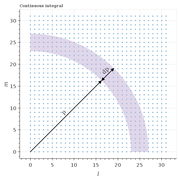
Using this formalism, we can express each wave in a cavity using three non-negative integers, : smaller integers represent longer wavelengths, while higher values represent shorter ones. We can represent these points in a graph, as shown in fig. 2.
Every point represents a wave-mode in the cavity: the points with the same modulo will have the same energy, or, more concisely, if we define , for the same value of , we have the same energy. The relation between and now becomes:
| (13) |
If we want to calculate the energy density, we have to sum the number of wave-modes with the same energy multiplied by their average energy and divide by volume:
| (14) |
where is the number of independent modes with wave-mode , is the average energy of that mode and the factor reflects the fact that each wave can have two independent polarizations. can be found using the Boltzmann distribution:
| (15) |
where and .
For the determination of , we need to estimate the number of wave-modes for a given energy: for an unconstrained system, when , we can suppose the wave-modes are so dense we can estimate them as the volume of a shell of a sphere with radius and thickness (as shown in fig. 2a):
| (16) |
where the factor reflects the fact we are only counting one octant (). We can now transform eq. 14 into a continuous sum, by frequency () or by wavelength ():
| (17) |
where
| (18) | ||||
| (19) |
Equations 18 and 19 are often presented in the form of power radiance, which can be found multiplying them by :
| (20) | ||||
| (21) |

3.2 Derivation of Planck’s law for constrained cavities
In section 3.1 we discussed the derivation of Planck’s law because now we will use the same principle to derive a similar equation for constrained cavities, where the wavelength sizes are comparable to the cavity dimensions. This time we can not transform eq. 14 in a continuous sum, but we have to handle it as an infinite discrete sum.
The value of can be found using the Boltzmann distribution:
| (22) |
while the value are the number of modes where , as shown in fig. 2b. Unfortunately, this value can not be calculated analytically but, if we define we can find the value of in the sequence A002102 (Sloane & Plouffe 1995). Using this definition, eqs. 19 and 21 become, respectively:
| (23) | ||||
| (24) |
where . Finally, we can find the sum for all the modes as:
| (25) | |||
| (26) |
3.3 Ratio between and
Using the results from the previous section and eqs. 8, 5 and 13, now it is possible to find a new expression for the function :
| (27) |
which can be expressed, using eq. 2, as a function of the object’s acceleration:
| (28) |
The term make very difficult any analytical solution of eq. 28, but it is possible to solve numerically, as shown in fig. 3. We can observe it is different from eq. 7: while we can observe that for , (classical case), and for , , as predicted by McCulloch 2007, but we also have a critical point at where we have a maximum value for .

This point would represent a stable point because, if we apply a small force to an object around this critical value, the shape of will stabilize the object’s acceleration. At the knowledge of the authors, no such behaviour was ever measured or predicted theoretically by other models.
4 Correction 2
In this section, we will discuss the radiation imbalance between the Cosmic and Rindler horizon. In McCulloch 2013, it is shown how applying eq. 7 to an object moving along the direction , as shown in fig. 4, there will be an imbalance between the radiation pressure on the right, limited by the cosmic horizon, and the radiation pressure on the left, limited by the nearer Rindler horizon.
This radiation pressure imbalance will cause a force reacting against any acceleration similar in behaviour to the classical inertia. It is shown in McCulloch 2013 (and partially corrected by Giné & McCulloch 2016), it is possible to express the force F as:
| (29) |
where is the object’s radiation cross-section, smaller than the physical cross-section, is the object’s volume and the modulus of the object’s acceleration.
It is also shown that, if we assume the particle a cube with size equal to the Planck’s length, , the model predicts an inertial mass of , which is greater than the Planck’s mass, (Giné & McCulloch 2016).
Our main concern is how the energy density substitution was performed in both McCulloch 2013 and Giné & McCulloch 2016:
| (30) |
In this substitution, the authors imply that only the peak wavelength of the Unruh spectrum contributes to the energy densities. In reality, this is deeply incorrect because for classical accelerations (i.e. ), the peak wavelength contributes only a tiny part of the overall energy density. We can define a new quantity , expressing the contribution of the peak wavelength to the radiation energy density as:
| (31) |
where is the wave-mode nearest to the peak wavelength, which can be calculated as:
| (32) |
In figure fig. 5, we can see the plot of over a range of different accelerations, and we can notice that for classical accelerations, eq. 30 it is wrong in principle.

5 Conclusions
In this paper we analysed two main articles (McCulloch 2007; McCulloch 2013) describing Quantized Inertia. We found two major flaws on the derivation presented, and we propose some corrections to address the found issues. Such flaws, if they do not invalidate, at least will require a major rethinking of the whole theory. In our article, we did not address the ability of Quantized Inertia to match the observational data.
We consider that speculative physics is fundamental for the constant progress of science: Quantized Inertia was often criticized because it does go against well-established principles such as the equivalence principle. We consider this should not be the criterion used to establish the validity of a theory: history teaches us that many scientific breakthroughs, encountered, in the beginning, strong resistance from the scientific community because they were against existing principles. For this reason, it is of fundamental importance that any new iteration of quantized inertia should have a stronger mathematical derivation and, eventually, a strategy for a practical experimental verification.
Acknowledgements
This work was supported by the research project PN19060104. We would like to thank our ATLAS group colleagues for the supportive working environment and in particular Prof. Călin Alexa for his guidance and support during the writing of this article. We would like also to thanks the Bokeh Development Team 2014 for the excellent tool used to create the plots of this paper and the reviewer of this article for his meaningful feedbacks and the intellectual integrity shown during the review process.
References
- Abercrombie et al. (2015) Abercrombie D., et al., 2015, Technical Report FERMILAB-PUB-15-282-CD, Dark Matter Benchmark Models for Early LHC Run-2 Searches: Report of the ATLAS/CMS Dark Matter Forum. CERN (arXiv:1507.00966)
- Aguirre et al. (2001) Aguirre A., Schaye J., Quataert E., 2001, ApJ, 561, 550
- Aprile et al. (2012) Aprile E., et al., 2012, Astropart. Phys., 35, 573
- Bokeh Development Team (2014) Bokeh Development Team 2014, Bokeh: Python library for interactive visualization. http://www.bokeh.pydata.org
- Giné & McCulloch (2016) Giné J., McCulloch M. E., 2016, Mod. Phys. Lett. A, 31, 1650107
- Hu et al. (2019) Hu J., Feng L., Zhang Z., Chin C., 2019, Nat. Phys., pp 1–9
- Koberlein (2017) Koberlein B., 2017, Quantized Inertia, Dark Matter, The EMDrive And How To Do Science Wrong, https://tinyurl.com/forbes-quantized-inertia
- Liu et al. (2019) Liu J., Liu Z., Wang L.-T., 2019, Phys. Rev. Lett., 122, 131801
- McCulloch (2007) McCulloch M. E., 2007, MNRAS, 376, 338
- McCulloch (2008) McCulloch M. E., 2008, MNRAS Lett., 389, L57
- McCulloch (2012) McCulloch M. E., 2012, Ap&SS, 342, 575
- McCulloch (2013) McCulloch M. E., 2013, EPL, 101, 59001
- McCulloch (2015) McCulloch M. E., 2015, EPL, 111, 60005
- McCulloch (2017) McCulloch M. E., 2017, Astrophys. Space Sci., 362, 57
- McCulloch (2018) McCulloch M. E., 2018, J. Space Expl., 7, 1
- Milgrom (1983) Milgrom M., 1983, ApJ, 270, 365
- Mitsou (2015) Mitsou V. A., 2015, J. Phys.: Conf. Ser., 651, 012023
- Rubin (1983) Rubin V. C., 1983, Science, 220, 1339
- Rubin et al. (1980) Rubin V. C., Ford Jr. W. K., Thonnard N., 1980, ApJ, 238, 471
- Sanders (2003) Sanders R. H., 2003, MNRAS, 342, 901
- Sloane & Plouffe (1995) Sloane N., Plouffe S., 1995, The Encyclopedia of Integer Sequences, 1st edition edn. Academic Press
- SuperCDMS Collaboration et al. (2014) SuperCDMS Collaboration et al., 2014, Phys. Rev. Lett., 112, 241302
- Unruh (1976) Unruh W. G., 1976, Phys. Rev. D, 14, 870