Precise Estimation of Renal Vascular Dominant Regions Using Spatially Aware Fully Convolutional Networks, Tensor-Cut and Voronoi Diagrams
Abstract
This paper presents a new approach for precisely estimating the renal vascular dominant region using a Voronoi diagram. To provide computer-assisted diagnostics for the pre-surgical simulation of partial nephrectomy surgery, we must obtain information on the renal arteries and the renal vascular dominant regions. We propose a fully automatic segmentation method that combines a neural network and tensor-based graph-cut methods to precisely extract the kidney and renal arteries. First, we use a convolutional neural network to localize the kidney regions and extract tiny renal arteries with a tensor-based graph-cut method. Then we generate a Voronoi diagram to estimate the renal vascular dominant regions based on the segmented kidney and renal arteries. The accuracy of kidney segmentation in 27 cases with 8-fold cross validation reached a Dice score of 95%. The accuracy of renal artery segmentation in 8 cases obtained a centerline overlap ratio of 80%. Each partition region corresponds to a renal vascular dominant region. The final dominant-region estimation accuracy achieved a Dice coefficient of 80%. A clinical application showed the potential of our proposed estimation approach in a real clinical surgical environment. Further validation using large-scale database is our future work.
Keywords:
kidney segmentation, fully convolutional networks, blood vessel segmentation, Voronoi diagram1 Introduction
Partial nephrectomy (PN), which has recently become one of the most common treatments for kidney cancer, can maintain a high residual renal function during surgery [37, 38, 46]. A critical problem during PN is that blood vessel clamping directly influences the quality of the surgery. However, PN surgery remains unstandardized. Due to the trade-off between residual renal function and surgical difficulty, it is difficult to design a criteria for PN surgery. In this work, we provide a better and more accurate computer-assisted diagnosis for PN by estimating the dominant region of each renal artery that facilitates identifying the blood vessels which feed the tumor. Physicians can easily make a surgical plan using such diagnosis information to determine the blood vessel clamping.
The feasibility of computer-aided diagnosis (CAD) for PN has been proven [42, 21, 19]. Ukimura et. al [42] performed PN on four patients who underwent 3D reconstruction for surgical navigation. The kidney surface was extracted by thresholding, the renal arteries were segmented by a simple region-growing method, and the tumor was manually segmented. Komai et al. [21] and Isotani et al. [19] used commercial software called “Vincent” to perform the computer analysis for PN clamping. The kidney was extracted by a semi-automatic region-growing method, and the renal arteries were segmented by applying facial detection technology using multi-phase information. Then the vascular dominant regions were estimated by applying a Voronoi diagram. All of the above research focused on the clinical study of CAD’s feasibility and its accuracy for PN surgery rather than engineering studies.
Precise estimation of the renal vascular dominant regions will contribute to more precise surgery, especially for PN surgeries. To precisely estimate the renal vascular dominant regions, precise kidney and renal artery segmentation is essential. In this work, we used a deep learning technique to extract the kidney and a tensor-based graph-cut approach to precisely segment the renal arteries. Finally, we used the automatically extracted kidney and renal arteries to estimate the vascular dominant regions using a Voronoi diagram.
Many organ segmentation methods have already been presented in the literature over the years. Statistical model methods are commonly used in abdominal organ segmentation problems. Lin et al. presented an elliptic candidate region to localize kidneys [22]. Zhou et al. constructed a prior shape model from a statistical atlas map for a liver segmentation problem [48]. Heimann et al. proposed deformable statistical shape models (SSMs) using atlas information [18]. Hybrid methods have also been proposed. Skalski et al. used a level-set method with ellipsoidal shape constraints for kidney segmentation [40]. Okada et al. used a combination of SSMs and an intensity model for a multi-organ segmentation problem [28]. Graphical models have also been widely used for organ segmentation. In our previous work [43], we used a graph-cut method to semi-automatically segment the kidney. Freiman et al. combined shape and graphical models to automatically extract the kidney region [12].
Machine learning techniques have also been applied to organ segmentation problems. Cuingnet et al. proposed a coarse-to-fine kidney segmentation method using random forests [10]. Support vector machines (SVMs) have also benn used for organ segmentation [1, 24]. Recently, researchers have adapted deep learning techniques to organ segmentation. Many state-of-the-art results have been achieved in the lungs [16], the pancreas [32], the liver [7], the head and neck [49], the mammogram mass [52], and the kidneys [41, 47].
The segmentation of renal arteries is another critical step in this work. Unlike other tissues like the liver, renal arteries have lower contrast that complicates the extraction of tiny blood vessels. Even though Hessian-based vesselness enhancement filters have been widely used in tubular structure segmentation [36, 11], they are unable to extract tiny blood vessels, especially of low contrast. Friman et al. presented novel template model tracking with a multiple hypothesis procedure [13]. Multiple hypothesis tracking schemes solved the early termination problem, but specifying a global terminal threshold is difficult. It thus leads to serious over-segmentation, especially for tiny blood vessels of low contrast. Recently, a deep learning technique extracted retinal blood vessels [15, 23, 14], showing its high potential for blood vessel segmentation. Since the deep learning technique is a data-demanding approach, it also requires large-scale annotated data for supervised learning. However, creating pixel-wise ground-truth labels for big-data is very labor-intensive, especially for 3D medical data.
The main contributions of this paper include the presentation of a fully automated and precise renal vascular dominant estimation approach using a deep learning method for kidney segmentation and a tensor-based graph-cut method for renal artery segmentation. As a preliminary study on CAD system for PN surgery, this work shows the potential of using medical image-processing techniques in improving precise PN surgeries.

2 Methods
In this section, we describe our proposed methods in detail. The workflow is shown in Fig. 1. First, the kidney regions are extracted using a deep learning approach. Second, a fine renal artery segmentation method is performed to segment the renal arteries inside the bounding-box of the kidney regions. After extracting the kidneys and the renal arteries, we estimate the vascular dominant regions with a Voronoi diagram. The relative statistics of the dominant regions are calculated for further surgical planning.
2.1 Kidney segmentation
In this work, we segment the kidney regions with a 3D U-Net-like fully convolutional network (FCN) architecture. U-Net architecture [30, 9], which is an extended version of FCN architecture, consists of a contracting path and a symmetric-expanding path. U-Net can achieve high segmentation accuracy with sparse annotated data [9]. Recently, many U-Net-like architectures have been proposed for segmentation tasks [33, 31, 26, 39, 49, 50, 51, 52].
Our network is based on previous 3D U-Net-like architecture [31, 39]. Roth et al. presented a U-Net-like architecture for organ segmentation on 3D medical images and achieved state-of-the-art segmentation results [31]. To tackle the GPU memory limitation problem, they used a sliding-windows strategy for large medical data. However, these cropped sub-volumes were trained independently, i.e., the spatial position information of the sub-volumes was ignored during training. Spatial information is a critical feature for organ segmentation because the relative spatial position of the human organs is generally unchanged between patients. Exploiting spatial information should improve organ segmentation accuracy. Many works have involved spatial information into networks. Brust et al. directly incorporated absolute position information into fully connected layers [5]. Akoury et al. presented a “Spatial PixelCNN” to impose spatial prior information to maintain the coherence of generated synthetic images [2]. Chen et al. incorporated spatial information into the end of an encoder (a bottom feature map) [6, 45]. Zhu et al. incorporated spatially structured learning in an adversarial FCN for mammographic mass segmentation [52].

Inspired by the work of Chen et al. [6], we introduce spatial position information into 3D U-Net-like architecture to impose the spatial information of each cropped sub-volume into our FCN architecture. Our proposed network is illustrated in Fig. 2. The backbone U-Net-like structure, which is based on a previous work [34], consists of four resolution levels. At each level, a skip connection links the contracting path and the corresponding symmetric-expanding path to provide higher resolution features to the symmetric-expanding path. Unlike original U-Net architecture, the skip connections in this network are summation instead of concatenation. Summation connections were first incorporated in U-Net by Roth et al. [33]. Their experimental results show that summation connections are slightly better than the original concatenation connections in the pancreas segmentation task. Each resolution level contains two series of convolutional layers, batch normalization and ReLU activation, in both the contracting and symmetric-expanding paths. The kernel sizes of all the convolutional and deconvolutional layers in our network are fixed to . The kernel size of the max pooling layers is fixed to .
We concatenated a three-channel feature map, including coordinates, to the bottom feature map to introduce the position information to FCN. The input coordinate information is the relative coordinates of the input sub-volume in the entire CT normalized to . Let be the three-channel spatial feature map, thus is defined as , where , , and denote coordinates of voxels in a sub-volume. denote width, height and depth of a CT image. Unlike a previous study [6] that only considered the center coordinates of the input sub-volume, we used all of the position information and resized the position volume (containing coordinate information) to a suitable input size.


Training
In this work, the input volume size of our network is fixed to . At each epoch, sub-volumes are cropped from the original CT volume and fed to the neural network. Here denotes the batch size. To achieve the best segmentation performance, we exploit the transfer learning technique and pre-train our model on a multi-organ segmentation dataset [33, 39], which doesn’t contain any kidney annotation, and fine-tune the model on our kidney dataset. This multi-organ segmentation dataset contains 377 cases, with 340 cases used for pre-training and 37 cases used for validation. The model with the best validation performance is used for fine-tuning. We used all pre-trained layers except the last classification layer. Fine-tuning was done on all layers.
Similar to previous works [30, 9, 33, 31, 39], we used a data-augmentation technique to increase the data variety and robustness. We performed both rigid and elastic transformations to each cropped sub-volume. Rigid transformation includes a translation with a range of pixels at each dimension and a rotation with range of . A B-spline deformation is employed as an elastic transformation to each sub-volume, like in previous works [9, 33, 31]. For each sub-volume, the deformation fields are randomly sampled from a uniform distribution with a maximum displacement of 3, and the number of B-spline control points in each dimension is set to 3 for all data-augmented experiments. In this work, we performed an in-place deformation operation. In a single iteration, we fed one original sub-volume and hybrid deformed sub-volumes to the network. A data-augmentation example is shown in Fig. 3. We individually show the rigid transformation, the elastic transformation, and the hybrid transformation, which combines the rigid and elastic transformations. Deformation is computed on-the-fly at each epoch during training.
In this work, we use pseudo Dice loss instead of conventional cross-entropy loss. Dice loss was first introduced in 2016 [26]. The definition of multi-class Dice coefficient loss used in this work can be written:
| (1) |
where and denote voxels from the ground-truth volume and segmentation results for class of total classes. is the total voxel amount of the volume.
Testing
The input volume size for testing is the same as in the training. We used a sliding-window strategy to obtain sub-volumes with size for testing. After predicting all of the sub-volumes, we restored these predictions to a complete 3D labeling data based on their respective positions. The probabilities of the overlapping regions were computed as average probabilities: , where denotes the probability of voxel from -th sub-volume, .
2.2 Renal artery segmentation
After extracting the kidney region from a CT volume, we performed a renal artery segmentation inside the VOI of the kidney region. Our previous work presented a tensor-based graph-cut blood vessel method called tensor-cut to segment the renal arteries [44]. This blood vessel segmentation method can segment tiny vascular structures, primarily designed for renal artery segmentation. Tensor-cut models the tubular structure as a second-order tensor using a Hessian matrix and builds a first-order Markov random field (MRF) using both geometry (tensors) and intensity information. Finally, a graph-cut approach is utilized to find the optimal MRF solution.


Vesselness enhancement filter
Vesselness enhancement filters have been widely used in the image processing field since they were proposed in 1998 by Frangi et al. [11] and Sato et al. [36]. By analyzing the eigenvalues of a Hessian matrix, these filters can obtain high response against contrast changes. The Hessian matrix of a 3-D image is given by
| (2) |
where stands for the second-order partial derivatives of image around voxel x. The following is Sato’s quantitative vesselness measure, which is specialized to 3-D images where the vessels are brighter than the background:
| (3) |
Utilizing a quantitative vesselness measure, we obtain the result of vesselness enhancement filter (Fig. 4). The enhanced vessel radius ranges from 1 to 2 mm.
A Hessian matrix can be treated as a second-order tensor. The vesselness enhancement filter transfers the higher dimensional tensor to 1-dimensional Euclidean measurement . This transformation introduces external errors. To tackle this problem, our tensor-cut algorithm models the Hessian matrix as a tensor and uses a Riemannian metric to measure the tensors.

Tensor-cut
The main idea of the tensor-cut method is to build a first-order MRF using both the geometry and intensity information and a graph-cut algorithm to extract the vascular structures. A simple tensor-cut workflow of tensor-cut is illustrated in Fig. 5. In this section, we briefly introduce the tensor-cut algorithm. More details are available [44].
As mentioned above, Hessian matrix can be treated as a second-order tensor . First, a vesselness enhancement filter is applied to the CT volume to obtain tensor field , where denotes the total voxel number.
To build a MRF with tensors, such tensor characteristics are needed as distance and mean value. We calculated them with an Euclidean metric [43]. Tensors resemble ellipsoids. The dissimilarity is calculated by the length of three principal axes, the angle, and the distance between center points. However, the Euclidean metric ignores the property by which tensors should lie on a manifold space. The tensor-cut method uses a Riemannian metric to measure the distance between two tensors. We used the affine invariant Riemannian metric presented by Pennec et al. [29]. A detailed mathematical proof is available [27, 29].
Instead of using a conventional histogram probability estimation approach, we used a Gaussian mixture model (GMM) [35]. Two GMMs are required for presenting the distribution of the foreground and background regions. GMM distribution under label is denoted by , and are the foreground and background labels. Thus, MRF’s energy function can be defined:
| (4) | ||||
where , , and are constant parameters to adjust the weight between the two smoothness terms and the tensor term. Two smoothness terms, and , present the dissimilarity of the intensity and tensor terms. As in previous works [35, 3, 4], we used the Potts model. Obviously, the biggest difference between the conventional graph-cut energy and tensor-cut energy functions is the introduction of the tensor term. By introducing an external tensor term, a more accurate MRF model can be obtained for tubular structure segmentation.
2.3 Estimation of vascular dominant region
We estimated the renal vascular dominant regions with a Voronoi diagram that is widely used for calculating vascular dominant regions [42, 21, 19]. Considering the capillaries along the arteries, each branch of the renal arteries is treated as a set of seed points of a Voronoi diagram instead of using the end points of arteries. Let be a branch of renal arteries, and define Voronoi cell function:
| (5) |
where image voxels are inside of kidney region extracted by the FCN approach. is the Euclidean distance between two points, and denotes the minimal Euclidean distance from point to vessel branch . This is a simple simulation of a real cell getting nutrition from blood vessels.

As demonstrated in Eq. 5, the main factors affecting the accuracy of a Voronoi diagram are kidney region and renal artery branches . In this work, we also provide different partition levels to help physicians better grasp the relationships among arteries, dominant regions, and tumors. Fig. 6 simply illustrates the Voronoi partition strategy used in this work. Fig. 6(a) shows the kidney region and its renal arteries. Green dots represent the entries of the renal arteries in the kidney. Fig. 6(b) shows the branch cluster result based on the entries of the arteries. All the artery branches downstream of the entries are clustered into the same group. This clustering idea is treated as a basic rule. Based on it, we generate different Voronoi partition levels by moving the bifurcation level of the vascular tree. As shown in Fig. 6(c), by moving the bifurcations of Fig. 6(b) one level upstream, we get new Voronoi partition results that show a coarser partition result. Moving the bifurcations one level downstream leads to a more precise partition result (Fig. 6(d)).
To get a quantitative measure for the estimation of the vascular dominant regions, we calculated the volume and the volume ratio of each dominant region denoted by and . If dominant regions are adjacent to a tumor, we also calculated the contact area of each adjacent region.
3 Materials
In this work, we used 27 pieces of abdominal contrast-enhanced CT volume data to evaluate the performance of our proposed method. The pixel spacing ranged from to mm, and slice pitch ranged from to mm. All 27 cases containing 54 kidneys were used to evaluate the accuracy of the kidney segmentation. Eight cases containing 14 kidneys were used for evaluating the dominant-region estimation. The ground truth of the kidneys was created by an engineer with medical knowledge. The ground truth of the renal artery was created by two engineers with medical knowledge. Since we directly used our previous method for blood vessel segmentation, we did not perform a quantitative evaluation for blood vessel segmentation in this work. Detailed experimental results are available in our previous work [44].


4 Experiments and Results
4.1 Kidney segmentation
We used an 8-fold cross-validation scheme to evaluate the accuracy of kidney segmentation. We divided all 27 CT volume data into train/validation/test splits at a ratio of . The model with the best validation performance is to be used for test. For a quantitative evaluation, we used three measures: the Dice Similarity coefficient (), Sensitivity (), and the Hausdorff distance (). is a commonly used measure in image segmentation. It is able to reflect the general segmentation ability. , also known as recall rate, measures the ability of the method to extract correct kidney regions. is introduced to measure the surface distance between segmentation results and ground truth. We use the metric to focus on segmentation accuracy of the kidney itself. Therefore, as post-processing, we extracted the top 2 largest connected components as kidney regions. is used to measure the post-processed segmentation results, to reflect the actual segmentation ability of end-to-end FCN, and are still used to measured the original segmentation results without any post-processing. , , and are defined as follows:
| (6) | ||||
where True Positive (TP), False Positive (FP), True Negative (TN), and False Negative (FN) were measured in a voxel-wise way. , where denotes the voxel coordinate that belongs to surface . and represent the surfaces of the manually annotated ground-truth label and post-processed segmentation results.
Experiments were performed on an NVIDIA Quadro P6000 with 24 GB memory. Training on 21 cases took about hours for 4000 iterations, and the testing phase took about five minutes for a single case. For all experiments in this work, we set the learning rate to , the batch size to 6, the sub-volume size to , and the epoch number to 4000 for fine-tuning and 16000 for pre-training.
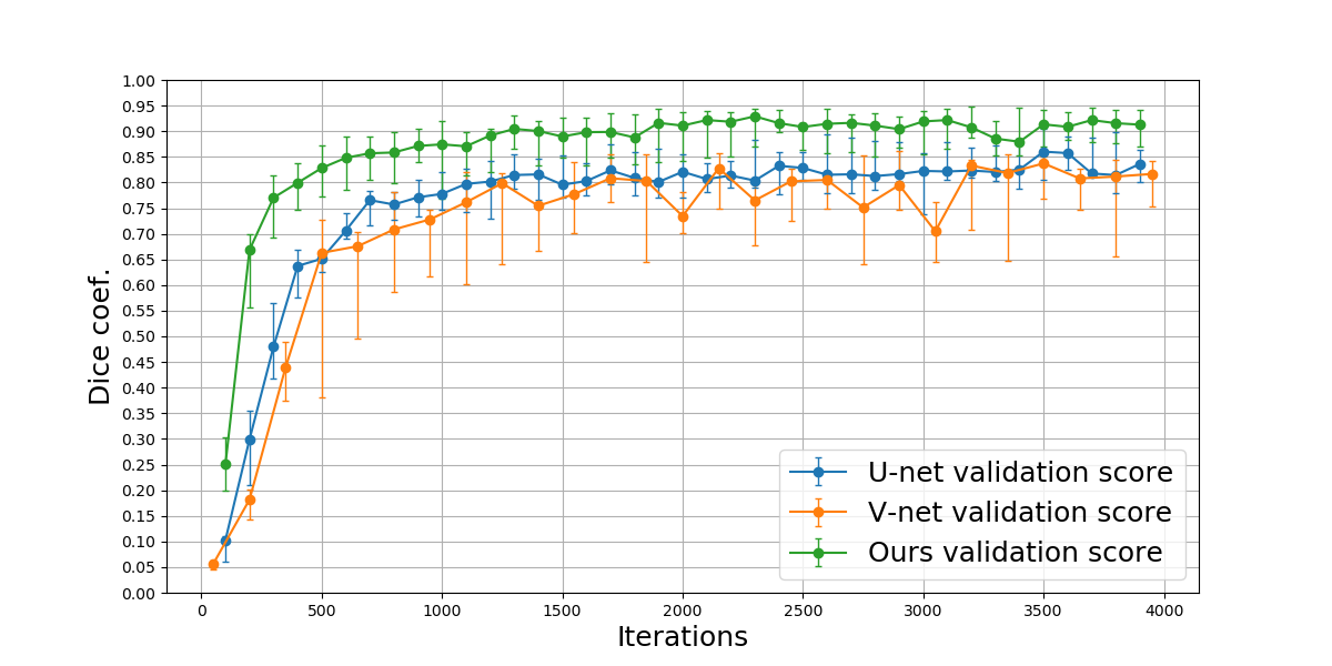
The FCN model was first pre-trained on a multi-organ dataset of seven organ labels, including the liver, the spleen, the stomach, and the pancreas. This multi-organ dataset did not contain any kidney labels. Its latest segmentation is given in previous work [39], which achieved an average accuracy of (excluding the background regions). The pre-training curve of our FCN model is plotted in Fig. 8(a). The maximum validation score was . The learning curve of the first fold’s fine-tuning on the kidney dataset is shown in Fig. 8(b). The maximum validation score of this fold was . To demonstrate the improvement made by introducing the spatial unit, we also evaluated the baseline U-Net [31], i.e. the proposed architecture without the spatial unit. Furthermore, we implemented a variant U-Net architecture, V-Net [26], for comparison on our kidney dataset. All comparison experiments have the same hyperparameter settings. Validation results of these three methods are shown in Fig. 9. The quantitative results of unseen test data of all 8-fold cross validations are shown in Table. 1. For reference, we also list several similar works on the kidney segmentation task, even though we used a different dataset and annotations. Two detailed segmentation examples using the proposed approach are shown in Fig. 10. Comparison segmentation results are shown in Fig. 11.
| Method | Modality | Case num | (%) | (%) | (mm) | ||||||||||||||
|---|---|---|---|---|---|---|---|---|---|---|---|---|---|---|---|---|---|---|---|
| Left | Right | Left | Right | ||||||||||||||||
| (1) In-house dataset | |||||||||||||||||||
| Atlas-based random forest [10] | CT |
|
|
|
- | ||||||||||||||
| Atlas-based graph-cut [8] |
|
100 (LOO) | - | - | |||||||||||||||
| CNN+MSL [47] |
|
|
90.5 | - | - | ||||||||||||||
| Shape-constrained Level-set [40] | CE-CT | 10 | 86.2 | - | 19.6 | ||||||||||||||
| 2D patch-based CNN [41] | CE-CT |
|
|
|
|
|
| ||||||||||||
| (2) Our kidney dataset | |||||||||||||||||||
| Baseline U-Net [31] | CE-CT | 27 (8-fold) |
|
|
|
|
| ||||||||||||
| V-Net [26] | CE-CT | 27 (8-fold) |
|
|
|
|
| ||||||||||||
| Ours | CE-CT | 27 (8-fold) |
|
|
|
|
| ||||||||||||

|
 |
|

|
 |
|
|---|---|---|---|---|---|
 |
|
 |
| ||
| Volume rendering | Axial slices | Volume rendering | Axial slices | ||


4.2 Renal artery segmentation
We performed renal artery segmentation on the VOIs of the kidney regions that were extracted using the bounding-boxes of the segmented kidneys. Tumors were segmented manually. Instead of using a Dice coefficient, as in previous work, we presented a centerline overlap () coefficient to evaluate the blood vessel segmentation accuracy. Using a blood vessel centerline to measure the segmentation accuracy was previously proposed [25]. The Dice coefficient is sensitive to volume variation. In tiny blood vessel segmentation problems, geometric topology error is more important than volume error. The coef. evaluates the overlapping of centerlines extracted from the ground-truth and segmentation results. Fig. 7 describes how to calculate the overlapping ratio. As demonstrated in previous work, the coef. of the segmentation results exceeded .
4.3 Estimation of dominant regions


We conducted a quantitative evaluation of the estimation of dominant regions in eight cases involving 14 kidneys. We measured each estimated dominant region’s Dice coef. with the ground truth. Since we cannot get the anatomical ground truth of the renal dominant regions, we used the ground truth of both kidney and renal artery to calculate a simulated ground truth of the dominant regions. The quantitative results are shown in Table 2. One partition example on the original CT volume is shown in Fig. 12.
| Case 1 | Case 2 | Case 3 | Case 4 | Case 5 | Case 6 | Case 7 | Case 8 | Mean | |||||||||||||||||||
| Kidney # | 2 | 2 | 2 | 2 | 1 | 1 | 2 | 2 | |||||||||||||||||||
| Regions # | 12 | 22 | 16 | 10 | 12 | 7 | 10 | 14 | |||||||||||||||||||
| Dice coef. (%) |
|
|
|
|
|
|
|
|
|


5 Discussion
In this work, we described a precise estimation approach for PN using a deep learning technique for kidney segmentation and a tensor-based graph-cut method for renal artery segmentation. We used our previously proposed “Tensor-cut” method for renal artery segmentation that can obtain over 80% segmentation accuracy [44]. For kidney segmentation, we presented an improved U-Net-like FCN architecture. The experimental results also demonstrate that better segmentation results were obtained by introduced the spatial information.
5.1 Kidney segmentation
As shown in Table 2, compared with other U-Net-like architectures, our proposed spatially aware FCN achieved better segmentation results. Figure 11 shows that the introduced spatial information effectively suppressed the FPs. Furthermore, our approach demonstrated competitive segmentation accuracy with related kidney segmentation methods. In this work, our and are directly measured on the segmentation results without any post-processing. A 2D patch-based CNN method [41] performed post-processing, including opening, closing and extraction of two largest connected components. Therefore, a comparison of is more useful for demonstrating our segmentation ability. Considering our limited dataset, we believe our proposed spatially aware FCN architecture has potential to achieve competitive results with state-of-the-art kidney-segmentation methods. Furthermore, the spatially aware unit can be easily incorporated in other architectures.
Although our network achieved good kidney segmentation results, its performance remains limited on such pathology patterns as kidney cysts and some late stage cancer. Several segmentation results are shown in Fig. 14. Figs. 14(a) and (b) show the under-segmented results of kidney cysts. Although the cyst regions have less effect on PN surgical plans, the segmentation of cysts can provide better diagnosis information. Fig. 14(c) shows a case with late-stage cancer, and the proposed method failed to segment the whole kidney. One reason is that we have only one case that contains this pattern in our dataset; increasing the data with this pattern may improve the segmentation performance. Among all 27 tested cases, two cases failed in segmentation (). This has also happened in other experiments using U-Net and V-Net. The major reason for this is that the slice thickness of these two failed cases is 2.0 mm, while that of all other cases ranges from 0.4 to 0.8 mm.


As shown in Fig. 15(a), the automatic segmentation of kidney regions contains the tumor region. Currently, we still need a manual segmentation process to extract tumors. One manually segmented result is shown in Fig. 15(b). A 5-mm margin was taken outside of the tumor for surgical safety. Much research has already been conducted on tumor segmentation using deep learning techniques [20, 17]. However, fine automatic segmentation of kidney tumors remains an essential future work.


5.2 Renal artery segmentation
As demonstrated in our previous work [44], the coef. of renal artery segmentation exceeded 80% and extracted about five generations of dichotomous branching that maximally extended from the abdominal aorta. This performance completely meets physician requirements for PN surgical planning. However, under-segmented renal arteries exist. As mentioned above, a renal artery is a critical step in our system. A variation of the segmented blood vessels will directly affect the result of the Voronoi diagram. We illustrated two examples with poor performance (Cases 2 and 6) in Fig. 16 to show the influence. Yellow arrows indicate the under-segmented renal arteries around the tumors. In our experiments, the under-segmented renal arteries slightly affected the estimation results of the dominant regions around the tumors. For Case 2, the renal arteries dominating the orange and green regions are clamped the same as the ground-truth. However, for Case 6, the blue region is over-estimated. Although the segmentation accuracy still need to be improved, the renal artery segmentation performance for dominant-region estimation is acceptable in this work.


| 1 | 2 | 3 | 4 | 5 | 6 | 7 | 8 | 9 | all | |
|---|---|---|---|---|---|---|---|---|---|---|
| Yellow | Blue | Light-green | Orange | Light-blue | Fuchsia | Green | Gray | Brown | ||
| () | 49596.7 | 22567.1 | 22311.6 | 14275.1 | 20234 | 1603.6 | 8986.3 | 460101 | 16719.3 | 160895 |
| Ratio (%) | 30.8 | 14.0 | 13.9 | 8.9 | 12.6 | 1.0 | 5.6 | 2.9 | 10.4 | 100 |
| () | 17.6 | – | – | – | 761.5 | 174.9 | 22.5 | – | – | 976.5 |
| Ratio (%) | 1.8 | – | – | – | 78.0 | 17.9 | 2.3 | – | – | 100 |
5.3 Estimation of dominant regions

We utilized a Voronoi diagram to estimate the dominant regions of the renal arteries. However, due to the limited size of annotated renal artery data, we could only perform quantitative validation on a small number of data (8 cases). The validation results from these 8 cases demonstrate that our estimation approach to the vascular dominant regions is generally correct. From this early study on the estimation of vascular dominant regions, we believe our proposed approach has the potential to improve estimation accuracy for dominant regions in clinical applications. More quantitative clinical validations of the recovery from ischemic damage to normal kidney function can be found in our previous work [46].
Figure 17 shows the computerized analysis result for PN surgical planning. Since surgeons only compared the computerized analysis result with a PN surgery screen in one case, we show one comparison result in this figure. The segmented renal arteries of the left kidney and the corresponding dominant regions are shown in Fig. 13. 5-mm margin was taken outside of the tumor for surgical safety. Two measures were investigated: the volume of the vascular dominant region () and the area of the dominant region adjacent to tumor (). The quantitative result is shown in Table 3. Nephrectomy surgery was performed using a selective artery clamping scheme shown in Fig. 17. We confirmed that four regions are adjacent to the tumor, and thus at most four blood vessel branches should be clamped based on our simulated results. Surgeons clamped two blood vessel branches that dominate regions 5 and 6. An operation report shows that slight bleeding remains in regions 1 and 7. However, a valuable trade-off is found between surgical quality and residual renal function. From surgeon feedback, our proposed approach helped surgeons build preoperative surgical plans and focus on critical arteries during operations.
6 Conclusion
This work presented a preliminary study on precise estimation approach for PN surgical planning. Our approach mainly consists of three parts: a spatially aware fully connected convolutional network to extract kidney regions, a tensor-based graph-cut method to segment renal arteries, and a Voronoi diagram to estimate the dominant regions. The automatic kidney and renal artery segmentation methods achieved competitive results with state-of-the-art methods in our in-house data. The vascular dominant region is essential information for selective artery clamping, and its precise estimation will contribute to better ways of recovering residual renal function. As a pilot study on the estimation of renal vascular dominant regions, our experimental results in 8 cases demonstrated that our estimation approach achieved reasonable accuracy. However, more clinical evaluations using large-scale database are needed to prove the feasibility of our approach for clinical PN surgical planning.
References
- Akbari and Fei [2012] Akbari, H., Fei, B., 2012. Automatic 3D segmentation of the kidney in mr images using wavelet feature extraction and probability shape model. In: Medical Imaging 2012: Image Processing. Vol. 8314. International Society for Optics and Photonics, p. 83143D.
- Akoury and Nguyen [2017] Akoury, N., Nguyen, A., 2017. Spatial pixelcnn: Generating images from patches. arXiv preprint arXiv:1712.00714.
- Boykov and Funka-Lea [2006] Boykov, Y., Funka-Lea, G., 2006. Graph cuts and efficient nd image segmentation. International journal of computer vision 70 (2), 109–131.
- Boykov and Jolly [2001] Boykov, Y. Y., Jolly, M.-P., 2001. Interactive graph cuts for optimal boundary & region segmentation of objects in nd images. In: Computer Vision, 2001. ICCV 2001. Proceedings. Eighth IEEE International Conference on. Vol. 1. IEEE, pp. 105–112.
- Brust et al. [2015] Brust, C.-A., Sickert, S., Simon, M., Rodner, E., Denzler, J., 2015. Convolutional patch networks with spatial prior for road detection and urban scene understanding. arXiv preprint arXiv:1502.06344.
- Chen et al. [2017] Chen, L., Xie, Y., Sun, J., Balu, N., Mossa-Basha, M., Pimentel, K., Hatsukami, T. S., Hwang, J.-N., Yuan, C., 2017. 3D intracranial artery segmentation using a convolutional autoencoder. In: Bioinformatics and Biomedicine (BIBM), 2017 IEEE International Conference on. IEEE, pp. 714–717.
- Christ et al. [2016] Christ, P. F., Elshaer, M. E. A., Ettlinger, F., Tatavarty, S., Bickel, M., Bilic, P., Rempfler, M., Armbruster, M., Hofmann, F., D’Anastasi, M., et al., 2016. Automatic liver and lesion segmentation in CT using cascaded fully convolutional neural networks and 3D conditional random fields. In: International Conference on Medical Image Computing and Computer-Assisted Intervention. Springer, pp. 415–423.
- Chu et al. [2013] Chu, C., Oda, M., Kitasaka, T., Misawa, K., Fujiwara, M., Hayashi, Y., Nimura, Y., Rueckert, D., Mori, K., 2013. Multi-organ segmentation based on spatially-divided probabilistic atlas from 3D abdominal CT images. In: International Conference on Medical Image Computing and Computer-Assisted Intervention. Springer, pp. 165–172.
- Çiçek et al. [2016] Çiçek, Ö., Abdulkadir, A., Lienkamp, S. S., Brox, T., Ronneberger, O., 2016. 3D u-net: learning dense volumetric segmentation from sparse annotation. In: International Conference on Medical Image Computing and Computer-Assisted Intervention. Springer, pp. 424–432.
- Cuingnet et al. [2012] Cuingnet, R., Prevost, R., Lesage, D., Cohen, L. D., Mory, B., Ardon, R., 2012. Automatic detection and segmentation of kidneys in 3D CT images using random forests. In: International Conference on Medical Image Computing and Computer-Assisted Intervention. Springer, pp. 66–74.
- Frangi et al. [1998] Frangi, A. F., Niessen, W. J., Vincken, K. L., Viergever, M. A., 1998. Multiscale vessel enhancement filtering. In: International Conference on Medical Image Computing and Computer-Assisted Intervention. Springer, pp. 130–137.
- Freiman et al. [2010] Freiman, M., Kronman, A., Esses, S. J., Joskowicz, L., Sosna, J., 2010. Non-parametric iterative model constraint graph min-cut for automatic kidney segmentation. In: International Conference on Medical Image Computing and Computer-Assisted Intervention. Springer, pp. 73–80.
- Friman et al. [2010] Friman, O., Hindennach, M., Kühnel, C., Peitgen, H.-O., 2010. Multiple hypothesis template tracking of small 3D vessel structures. Medical image analysis 14 (2), 160–171.
- Fu et al. [2016a] Fu, H., Xu, Y., Lin, S., Wong, D. W. K., Liu, J., 2016a. Deepvessel: Retinal vessel segmentation via deep learning and conditional random field. In: International Conference on Medical Image Computing and Computer-Assisted Intervention. Springer, pp. 132–139.
- Fu et al. [2016b] Fu, H., Xu, Y., Wong, D. W. K., Liu, J., 2016b. Retinal vessel segmentation via deep learning network and fully-connected conditional random fields. In: Biomedical Imaging (ISBI), 2016 IEEE 13th International Symposium on. IEEE, pp. 698–701.
- Harrison et al. [2017] Harrison, A. P., Xu, Z., George, K., Lu, L., Summers, R. M., Mollura, D. J., 2017. Progressive and multi-path holistically nested neural networks for pathological lung segmentation from CT images. In: International Conference on Medical Image Computing and Computer-Assisted Intervention. Springer, pp. 621–629.
- Havaei et al. [2017] Havaei, M., Davy, A., Warde-Farley, D., Biard, A., Courville, A., Bengio, Y., Pal, C., Jodoin, P.-M., Larochelle, H., 2017. Brain tumor segmentation with deep neural networks. Medical image analysis 35, 18–31.
- Heimann and Meinzer [2009] Heimann, T., Meinzer, H.-P., 2009. Statistical shape models for 3D medical image segmentation: a review. Medical image analysis 13 (4), 543–563.
- Isotani et al. [2015] Isotani, S., Shimoyama, H., Yokota, I., China, T., Hisasue, S.-i., Ide, H., Muto, S., Yamaguchi, R., Ukimura, O., Horie, S., 2015. Feasibility and accuracy of computational robot-assisted partial nephrectomy planning by virtual partial nephrectomy analysis. International Journal of Urology 22 (5), 439–446.
- Kamnitsas et al. [2017] Kamnitsas, K., Ledig, C., Newcombe, V. F., Simpson, J. P., Kane, A. D., Menon, D. K., Rueckert, D., Glocker, B., 2017. Efficient multi-scale 3D CNN with fully connected CRF for accurate brain lesion segmentation. Medical image analysis 36, 61–78.
- Komai et al. [2014] Komai, Y., Sakai, Y., Gotohda, N., Kobayashi, T., Kawakami, S., Saito, N., 2014. A novel 3-dimensional image analysis system for case-specific kidney anatomy and surgical simulation to facilitate clampless partial nephrectomy. Urology 83 (2), 500–507.
- Lin et al. [2006] Lin, D.-T., Lei, C.-C., Hung, S.-W., 2006. Computer-aided kidney segmentation on abdominal CT images. IEEE transactions on information technology in biomedicine 10 (1), 59–65.
- Liskowski and Krawiec [2016] Liskowski, P., Krawiec, K., 2016. Segmenting retinal blood vessels with deep neural networks. IEEE transactions on medical imaging 35 (11), 2369–2380.
- Liu et al. [2007] Liu, X., Samarabandu, J., Li, S., Ross, I., Garvin, G., 2007. A learning-based automatic clinical organ segmentation in medical images. In: Medical Imaging 2007: Image Processing. Vol. 6512. International Society for Optics and Photonics, p. 65120Y.
- Metz et al. [2008] Metz, C., Schaap, M., van Walsum, T., van der Giessen, A., Weustink, A., Mollet, N., Krestin, G., Niessen, W., 2008. 3D segmentation in the clinic: A grand challenge ii-coronary artery tracking. Insight Journal 1 (5), 6.
- Milletari et al. [2016] Milletari, F., Navab, N., Ahmadi, S.-A., 2016. V-net: Fully convolutional neural networks for volumetric medical image segmentation. In: 2016 Fourth International Conference on 3D Vision (3DV). IEEE, pp. 565–571.
- Moakher [2005] Moakher, M., 2005. A differential geometric approach to the geometric mean of symmetric positive-definite matrices. SIAM Journal on Matrix Analysis and Applications 26 (3), 735–747.
- Okada et al. [2015] Okada, T., Linguraru, M. G., Hori, M., Summers, R. M., Tomiyama, N., Sato, Y., 2015. Abdominal multi-organ segmentation from CT images using conditional shape–location and unsupervised intensity priors. Medical image analysis 26 (1), 1–18.
- Pennec et al. [2006] Pennec, X., Fillard, P., Ayache, N., 2006. A riemannian framework for tensor computing. International Journal of computer vision 66 (1), 41–66.
- Ronneberger et al. [2015] Ronneberger, O., Fischer, P., Brox, T., 2015. U-net: Convolutional networks for biomedical image segmentation. In: International Conference on Medical image computing and computer-assisted intervention. Springer, pp. 234–241.
- Roth et al. [2018a] Roth, H., Oda, M., Shimizu, N., Oda, H., Hayashi, Y., Kitasaka, T., Fujiwara, M., Misawa, K., Mori, K., 2018a. Towards dense volumetric pancreas segmentation in CT using 3d fully convolutional networks. In: Medical Imaging 2018: Image Processing. Vol. 10574. International Society for Optics and Photonics, p. 105740B.
- Roth et al. [2018b] Roth, H. R., Lu, L., Lay, N., Harrison, A. P., Farag, A., Sohn, A., Summers, R. M., 2018b. Spatial aggregation of holistically-nested convolutional neural networks for automated pancreas localization and segmentation. Medical image analysis 45, 94–107.
- Roth et al. [2018c] Roth, H. R., Oda, H., Zhou, X., Shimizu, N., Yang, Y., Hayashi, Y., Oda, M., Fujiwara, M., Misawa, K., Mori, K., 2018c. An application of cascaded 3D fully convolutional networks for medical image segmentation. Computerized Medical Imaging and Graphics.
- Roth et al. [2018d] Roth, H. R., Shen, C., Oda, H., Oda, M., Hayashi, Y., Misawa, K., Mori, K., 2018d. Deep learning and its application to medical image segmentation. Medical Imaging Technology 36 (2), 63–71.
- Rother et al. [2004] Rother, C., Kolmogorov, V., Blake, A., 2004. Grabcut: Interactive foreground extraction using iterated graph cuts. In: ACM transactions on graphics (TOG). Vol. 23. ACM, pp. 309–314.
- Sato et al. [1998] Sato, Y., Nakajima, S., Shiraga, N., Atsumi, H., Yoshida, S., Koller, T., Gerig, G., Kikinis, R., 1998. Three-dimensional multi-scale line filter for segmentation and visualization of curvilinear structures in medical images. Medical image analysis 2 (2), 143–168.
- Shao et al. [2011] Shao, P., Qin, C., Yin, C., Meng, X., Ju, X., Li, J., Lv, Q., Zhang, W., Xu, Z., 2011. Laparoscopic partial nephrectomy with segmental renal artery clamping: technique and clinical outcomes. European urology 59 (5), 849–855.
- Shao et al. [2012] Shao, P., Tang, L., Li, P., Xu, Y., Qin, C., Cao, Q., Ju, X., Meng, X., Lv, Q., Li, J., et al., 2012. Precise segmental renal artery clamping under the guidance of dual-source computed tomography angiography during laparoscopic partial nephrectomy. European urology 62 (6), 1001–1008.
- Shen et al. [2018] Shen, C., Roth, H. R., Oda, H., Oda, M., Hayashi, Y., Misawa, K., Mori, K., 2018. On the influence of dice loss function in multi-class organ segmentation of abdominal CT using 3d fully convolutional networks. arXiv preprint arXiv:1801.05912.
- Skalski et al. [2017] Skalski, A., Heryan, K., Jakubowski, J., Drewniak, T., 2017. Kidney segmentation in CT data using hybrid level-set method with ellipsoidal shape constraints. Metrology and Measurement Systems 24 (1), 101–112.
- Thong et al. [2016] Thong, W., Kadoury, S., Piché, N., Pal, C. J., 2016. Convolutional networks for kidney segmentation in contrast-enhanced CT scans. Computer Methods in Biomechanics and Biomedical Engineering: Imaging & Visualization, 1–6.
- Ukimura et al. [2012] Ukimura, O., Nakamoto, M., Gill, I. S., 2012. Three-dimensional reconstruction of renovascular-tumor anatomy to facilitate zero-ischemia partial nephrectomy. European urology 61 (1), 211–217.
- Wang et al. [2016a] Wang, C., Kagajo, M., Nakamura, Y., Oda, M., Yoshino, Y., Yamamoto, T., Mori, K., 2016a. Precise renal artery segmentation for estimation of renal vascular dominant regions. In: Medical Imaging 2016: Image Processing. Vol. 9784. International Society for Optics and Photonics, p. 97842M.
- Wang et al. [2016b] Wang, C., Oda, M., Hayashi, Y., Yoshino, Y., Yamamoto, T., Frangi, A. F., Mori, K., 2016b. Tensor-based graph-cut in riemannian metric space and its application to renal artery segmentation. In: International Conference on Medical Image Computing and Computer-Assisted Intervention. Springer, pp. 353–361.
- Wolterink et al. [2015] Wolterink, J. M., Leiner, T., Viergever, M. A., Išgum, I., 2015. Automatic coronary calcium scoring in cardiac ct angiography using convolutional neural networks. In: International Conference on Medical Image Computing and Computer-Assisted Intervention. Springer, pp. 589–596.
- Yoshino et al. [2015] Yoshino, Y., Yamamoto, T., Funahashi, Y., Oda, M., Kagajo, M., Wang, C., Mori, K., Gotoh, M., 2015. Computational analysis of recovery from ischemic damage to kidney function undergoing robotic partial nephrectomy for renal tumor. In: Supplement of Journal of Endourology. pp. 916–924.
- Zheng et al. [2017] Zheng, Y., Liu, D., Georgescu, B., Xu, D., Comaniciu, D., 2017. Deep learning based automatic segmentation of pathological kidney in CT: Local versus global image context. In: Deep Learning and Convolutional Neural Networks for Medical Image Computing. Springer, pp. 241–255.
- Zhou et al. [2006] Zhou, X., Kitagawa, T., Hara, T., Fujita, H., Zhang, X., Yokoyama, R., Kondo, H., Kanematsu, M., Hoshi, H., 2006. Constructing a probabilistic model for automated liver region segmentation using non-contrast x-ray torso ct images. In: International Conference on Medical Image Computing and Computer-Assisted Intervention. Springer, pp. 856–863.
- Zhu et al. [2018a] Zhu, W., Huang, Y., Zeng, L., Chen, X., Liu, Y., Qian, Z., Du, N., Fan, W., Xie, X., 2018a. Anatomynet: Deep learning for fast and fully automated whole-volume segmentation of head and neck anatomy. Medical physics.
- Zhu et al. [2018b] Zhu, W., Liu, C., Fan, W., Xie, X., 2018b. Deeplung: Deep 3d dual path nets for automated pulmonary nodule detection and classification. In: 2018 IEEE Winter Conference on Applications of Computer Vision (WACV). IEEE, pp. 673–681.
- Zhu et al. [2018c] Zhu, W., Vang, Y. S., Huang, Y., Xie, X., 2018c. Deepem: Deep 3d convnets with em for weakly supervised pulmonary nodule detection. In: International Conference on Medical Image Computing and Computer-Assisted Intervention. Springer, pp. 812–820.
- Zhu et al. [2018d] Zhu, W., Xiang, X., Tran, T. D., Hager, G. D., Xie, X., 2018d. Adversarial deep structured nets for mass segmentation from mammograms. In: 2018 IEEE 15th International Symposium on Biomedical Imaging (ISBI 2018). IEEE, pp. 847–850.