Image Steganography using Gaussian Markov Random Field Model

Let us first give the notations and conventions used throughout the paper. The calligraphic fonts will be used solely for sets (occasionally, other symbols may also be used for sets in the interest of ease presentation), random variables will be typeset in capital letters, while their corresponding realizations will be in lower cases. Vectors and matrices will always typeset in bold fonts. Cover and stego images ${\bf{c}}=({c_{k}})$ and ${\bf{s}}=({s_{k}})$ are addressed by their one-dimensional index set ${{\cal S}}=\{1,2,\cdots,K\}$, where ${c_{k}}$ and ${s_{k}}$ $\in\left\{{0,1,\cdots,G-1}\right\}$ and $G=256$ for 8-bit grayscale images. We also use the Iverson bracket, $\left[P\right]$, defined as $\left[P\right]$=1 when the statement $P$ is true and zero otherwise.

Let ${\cal S}$ be a set of $n$ discrete sites, i.e., ${{\cal S}}=\{1,2,\cdots,n\}$, and ${\bf{Z}}=({Z_{1}},{Z_{2}},\cdots,{Z_{n}})$ be a family of random variables defined on set ${\cal S}$, the neighborhood system for $\bf{Z}$ is defined as

where ${\cal N}_{k}$ is the collection of sites neighboring to $k$ for which $k\notin{\cal N}_{k}$ and $k\in{{{\cal N}}_{l}}\Leftrightarrow l\in{{{\cal N}}_{k}}$. In MRF, the ordering of sites are not important, and their relationship is determined by the corresponding neighborhood system ${\cal N}$. A subset ${c}\in{{\cal S}}$ is known as a clique if each pair of different elements from $c$ is neighbor. In this paper, unless stated otherwise, we only consider the four-element cross neighborhood and the associated two-pixel cliques of horizontally or vertically neighboring pixels as shown in Fig. 1.

For the family of random variables $\bf{Z}$, each random variable $Z_{k}$ takes the value ${z_{k}}\in{\mathbb{R}}$ with probability $p({Z_{k}}={z_{k}})$, and the joint event $({Z_{1}}={z_{1}},\cdots,{Z_{n}}={z_{n}})$ is abbreviated as $\bf{Z}=\bf{z}$ with the probability $p(\bf{Z}=\bf{z})$. $\bf{Z}$ is known as a Markov Random Field (MRF) on ${\cal S}$ with respect to the neighborhood system ${\cal N}$ if and only if (iff) the following two conditions are satisfied [18]:

The Markovianity says that the probability of a local event at $k$ conditioned on all the remaining events is equivalent to that conditioned on the events at the neighbors of $k$. A random vector ${\bf{Z}}={({Z_{1}},{Z_{2}},\cdots,{Z_{n}})^{T}}\in{{\mathbb{R}}^{n}}$ is called a Gaussian MRF (GMRF) w.r.t. a labeled graph ${{\cal G}}=({{\cal V}},{{\cal E}})$ (${\cal V}$: Vertices; ${\cal E}$: Edges) with mean ${\bm{\mu}}$ and precision matrix ${\bm{\Sigma}}^{-1}>0$ , iff it is Gaussian distributed with the form [19]:

and ${\bm{\Sigma}}_{k,l}^{-1}\neq 0\Leftrightarrow\left\{{k,l}\right\}\in{\rm{{\cal E}}}$ for all $k\neq l$.

Once the condition for Positivity is satisfied, which is always true for practical applications, the joint probability $p({\bf{z}})$ is uniquely determined by its local conditional probabilities [20]. In other words, the $p({\bf{z}})$ is characterized with the distributions of all involved cliques associated with the given neighborhood system. We then proceed to develop the cover and stego image model based on the distributions of horizontally or vertically neighboring two-pixel clique in the next two subsections.

As will be discussed later in Section III, a GMRF model with four-element cross neighborhood system is utilized to model the cover images in this paper. For a given uniform scalar quantizer ${Q_{\Delta}}$ with quantization step ${\Delta}$, the cover is quantized to a zero mean jointly distributed Gaussian ${Q_{\Delta}}(N({\bf{0}},{\bf{\Sigma}}))$. Without loss of generality, in practice, the mean of the image cover is removed from each pixel, and the ${\Delta}$ is generally set to be 1, in the interest of simplicity. According to [21], for a multivariate Gaussian random variable, its marginal variables are also Gaussian distributed, as a result, both the single pixel and the horizontally or vertically neighboring pixel pair in the cover images, which are associated with the adopted neighborhood system, are assumed to be Gaussian and jointly Gaussian distributed, respectively. Let ${\bf{X}}=\{{{\bf{X}}^{1}},{{\bf{X}}^{2}},\cdots,{{\bf{X}}^{M}}\}$ be the sequence of all involved two-pixel cliques in the cover image, for the $m^{th}$ clique ${{\bf{X}}^{m}}={\left[{X_{1}^{m},X_{2}^{m}}\right]^{T}}$, we have

that is

where ${{\bf{\Sigma}}^{m}}$ and $({\bf{\Sigma}}^{m})^{-1}$ are the covariance and precision matrices, resepctively. The corresponding Probability Mass Function (p.m.f) for the $m^{th}$ clique can be computed under the fine quantization step $\Delta$,

Let $x_{1}^{m}=i\Delta,x_{2}^{m}=j\Delta$, the p.m.f $p_{i,j}^{m}$ for the $m^{th}$ clique can then be evaluated by incorporating the Mean Value Theorem (MVT):

where $i^{\prime}\in(i-0.5,i+0.5)$ and $j^{\prime}\in(j-0.5,j+0.5)$.

Unlike the MG [4] and MiPOD [7] with mutually inde-pendent embedding, we take into account the interactions among embedding changes of neighboring pixels when modifying the cover ${\bf{x}}=({x_{k}})$ to stego ${\bf{y}}=({y_{k}})$, where ${x_{k}}$ and ${y_{k}}$ are the $k^{th}$ cover and stego pixels, respectively. However, to simplify the problem, the same symmetric ternary embedding model as shown in Fig. 2 is adopted throughout the paper, i.e.,

where the change probability $\beta_{k}^{+}=\beta_{k}^{-}={\beta_{k}}$, ${\beta_{k}}\in[0,{1\mathord{\left/{\vphantom{13}}\right.\kern-1.2pt}3}]$ is the change probability for the $k^{th}$ pixel of cover $\bf{x}$.

With the symmetric embedding model, the two-pixel cover clique sequence ${\bf{X}}=\{{{\bf{X}}^{m}}\}$ with p.m.f ${p^{m}}(x_{1}^{m},x_{2}^{m})$ is changed to stego clique sequence ${\bf{Y}}=\{{{\bf{Y}}^{m}}\}$ with p.m.f ${q^{m}}(y_{1}^{m},y_{2}^{m})$, where $m=1,2\cdots,M$. Let $\beta_{1}^{m}$ and $\beta_{2}^{m}$ be the change probabilities for pixels $X_{1}^{m}$ and $X_{2}^{m}$ in the $m^{th}$ clique, and ${\bf{X}}_{i,j}^{m}$ and ${\bf{Y}}_{i,j}^{m}$ denote the $m^{th}$ two-pixel cover and stego cliques which take the value $[i,j]$, respectively. Under ternary embedding with symmetric changes, there are totally 9 embedding change types as shown in Fig. 3,

where $\beta_{1}^{m}$ and $\beta_{2}^{m}$ $\in\left[{0,{1\mathord{\left/{\vphantom{13}}\right.\kern-1.2pt}3}}\right]$. Therefore, the p.m.f for the $m^{th}$ clique in stego image can be written as

where $p_{i,j}^{m}$ and $q_{i,j}^{m}$ are the probability values for the $m^{th}$ two-pixel cover and stego cliques which take the value $[i,j]$, respectively.

For a two-pixel cover clique ${\bf{X}}={[{X_{1}},{X_{2}}]^{T}}$, the embedding modifies the two pixels with probabilities ${\bm{\beta}}={\left[{{\beta_{1}},{\beta_{2}}}\right]^{T}}$, changing to the stego clique ${\bf{Y}}={[{Y_{1}},{Y_{2}}]^{T}}$. Note that we omit the superscript $``m"$ for simplicity. For small change probabilities ${\bm{\beta}}$, the KL-divergence between cover and stego cliques can be well approximated with its leading quadratic terms (detailed derivations see Appendix A-1):

where ${F_{P}}$ and $F_{Q}^{\bm{\beta}}$ are the p.m.f of the two-pixel cover clique and stego clique, respectively, ${\nabla^{2}}D({\bf{0}})$ is the second order partial derivative of $D$ w.r.t ${\bm{\beta}}$ when ${\bm{\beta}}=\bf{0}$. Similar to the result in [22], ${\nabla^{2}}D({\bm{\beta}})$ is also proportional to the Fisher information matrix ${{\bf{I}}_{2}}({\bm{\beta}})$ at ${\bm{\beta}}={\bf 0}$ (for proof see Appendix A-1), i.e.,

where ${{\bf{I}}_{2}}({\bf{0}})$ is the binary steganographic Fisher Information Matrix (FIM)

where

Furthermore, by incorporating (10) and (7) for the derivation of (14) through Taylor expansion, we can derive the closed-form expression for FIM ${{\bf{I}}_{2}}({\bf{0}})$ (refer to Appendix A-2 for detailed derivations):

where $\Omega_{i,j}^{1}=({p_{i-1,j}}+{p_{i+1,j}}-2{p_{i,j}})$, $\Omega_{i,j}^{2}=({p_{i,j-1}}+{p_{i,j+1}}-2{p_{i,j}})$, and by applying the result in (7), for fine quantization step $\Delta$, $f(i^{\prime}\Delta,j^{\prime}\Delta)\approx f(i\Delta,j\Delta)$, where $i^{\prime}\in(i-0.5,i+0.5)$, $j^{\prime}\in(j-0.5,j+0.5)$, thus we further have

where $f(x_{1},x_{2})$ is the bivariate Gaussian p.d.f as shown in (5). It is observed that $\Omega_{i,j}^{1}$ and $\Omega_{i,j}^{2}$ are linearly proportional to the second order partial derivatives of ${f}({x_{1}},{x_{2}})$ (bivariate Gaussian for two-pixel clique) w.r.t. ${x_{1}}$ and ${x_{2}}$ at ${x_{1}}=i\Delta$ and ${x_{2}}=j\Delta$, respectively. On the other hand, the second order partial derivatives of ${f}({x_{1}},{x_{2}})$ in (16) can be easily obtained according to (5), i.e.,

where ${\gamma_{1,1}}$, ${\gamma_{1,2}}$, ${\gamma_{2,1}}$ and ${\gamma_{2,2}}$ are the components of the precision matrix ${{\bm{\Sigma}}^{-1}}$ in (5). Based on these, substituting (17) into (16) at ${x_{1}}=i\Delta,{x_{2}}=j\Delta$, then we can have the FIM ${\bf{I}}_{2}(\bf{0})$ (${\lim\Delta\to 0}$)

It is readily seen that the elements of FIM in (13) can be represented in terms of ${2^{th}}$ order and ${4^{th}}$ order moments of bivariate Gaussian $\bf{X}$, which, according to Isserlis’ theorem [23], can be represented as

where ${\sigma_{1,2}}$ is the covariance of $X_{1}$ and $X_{2}$, ${\sigma_{1,1}}$ and ${\sigma_{2,2}}$ are the variance of $X_{1}$ and $X_{2}$, respectively. Therefore, we finally obtain the FIM ${{\bf{I}}_{2}}({\bf 0})$ as follows:

where ${\rho_{1,2}}={{{\sigma_{1,2}}}\mathord{\left/{\vphantom{{{\sigma_{1,2}}}{\sqrt{{\sigma_{1,1}}{\sigma_{2,2}}}}}}\right.\kern-1.2pt}{\sqrt{{\sigma_{1,1}}\cdot{\sigma_{2,2}}}}}$ is the correlation coefficient of $X_{1}$ and $X_{2}$.

Thus far, we can rewrite the KL-divergence between a pair of two-pixel cover and stego cliques by taking advantage of (11), (12), (13) and (22),

It is observed that the KL-divergence of a two-pixel clique is relevant to the correlation coefficient, variances and change probabilities of pixels in the clique, among which, the correlation coefficients for each neighboring pixel pair in the involved cliques are the predominant parameters to be determined for the incorporated Gaussian MRF model. In general, the performance of the proposed MRF based steganographic scheme is heavily dependent on the estimation accuracy of the model parameters. To this end, we follow in spirit the scheme in MiPOD [7] to estimate the pixel variance and the correlation coefficient of neighboring pixels in a clique, which will be illustrated later in next subsection.

In [7], Sedighi et al. proposed an elegant pixel variance estimator to build the underlying multivariate independent Gaussian model, which leads to notable performance improvement over its predecessor MG [4]. The variance estimator consists of two steps, that is: 1) suppress the image content using a denoising filter to obtain the residual image; 2) fit a local parametric model to the neighbors of each residual to obtain its variance estimation.

In light of its effectiveness, the same strategy is also generalized to develop the covariance estimator for the involved Gaussian MRF model. For the 8-bit grayscale cover image with original pixel values ${\bf{c}}=({c_{1}},{c_{2}},\cdots,{c_{n}})$, we obtain the residual ${\bf{r}}$ of the cover ${\bf{c}}$ using a two-dimensional wiener filter $F$: ${\bf{r}}={\bf{c}}-F({\bf{c}})$. Then we utilize a local parametric model to estimate the pixel variance by blockwise Maximum Likelihood Estimation (MLE) [24]. For the ${n^{th}}$ residual ${{{r}}_{n}}$ in cover ${\bf{c}}$, we fit the local parametric model [25] to the $p\times p$ neighbors of ${{{r}}_{n}}$ and model the residual expectation within the associated $p\times p$ block as follows:

where ${{\bf{r}}_{n}}$ denotes the residual values inside the $p\times p$ block surrounding the ${n^{th}}$ residual ${{{r}}_{n}}$, which is a column vector of size ${p^{2}}\times 1$, ${\bf{G}}$ is the matrix of size ${p^{2}}\times q$ which defines the adopted parametric model, ${{\bf{a}}_{n}}$ is the parameter vector of size $q\times 1$, and ${{\bm{\xi}}_{n}}$ is the noise vector of the model with the variance and covariance to be estimated. Under the assumption of Gaussian noise, the estimation of the residual ${{\bf{r}}_{n}}$ is

In general, we could assume the residuals within the $p\times p$ block centered on ${r_{n}}$ exhibit the similar statistical characteristics, i.e., they could be regarded as the multiple samples of ${r_{n}}$. Therefore, the covariance of neighboring pixels ${{{c}}_{m}}$ and ${{{c}}_{n}}$ in a clique can be well estimated as

Similarly, we have the variance estimation for pixel ${{{c}}_{n}}$, i.e.,

Given the variance and covariance estimations for pixels ${{{c}}_{m}}$ and ${{{c}}_{n}}$, we can readily obtain the correlation coefficient between them, i.e.,

Considering the numerical stability and computational efficiency, we set adequate bounds for $\rho$ and ${\sigma_{n,n}}$, i.e., $\rho=min(\rho,0.99*sign(\rho))$ and ${\sigma_{n,n}}=max(0.01,{\sigma_{n,n}})$.

With the formulation of KL-divergence of a two-pixel clique in (23), we then further derive the total KL-divergence between cover and stego by incorporating the given Gaussian MRF with four-element cross neighborhood as shown in Fig. 1, where the image of size $M\times N$ is decomposed into two interleaved subimages (sublattices) ${\cal A}$ (“$+$”) and ${\cal B}$ (“$\times$”), i.e.,

where $1\leq k\leq M\times N$.

For any pixel ${X_{s}}$ in subimage ${\cal A}$ (the same for ${\cal B}$), there are four cliques associated with it, i.e., ${{\bf{X}}_{{s},{t}}}=[{X_{s}},{X_{t}}]^{T}$, $t=1,\cdots,4$, which constitute a 4-ary clique tree denoted by ${T_{s}}=\{X_{s},X_{1},X_{2},X_{3},X_{4}\}$, as shown in Fig. 1. With given ${X_{s}}$ (or ${\beta_{s}}$) in ${\cal A}$, the other four pixels (${X_{t}}$) in cliques ${{\bf{X}}_{{s},{t}}}$ ($t=1,\cdots,4$) of ${T_{s}}$ are conditionally independent under the proposed Gaussian MRF model with four-element cross neighborhood. We then obtain the KL-divergence for clique tree ${T_{s}}$ (refer to Appendix B for details)

where ${{\cal C}}=\left\{{{\rm{\{}}{X_{s}},{X_{t}}{\rm{\}}},|t=1,\cdots 4}\right\}$, ${{\bm{\beta}}_{c}}={[{\beta_{X_{s}}},{\beta_{X_{t}}}]^{T}}$, ${{\bf{I}}_{2,{c}}}({\bf{0}})$ is binary FIM for clique ${c}$, $I_{1,{{X_{s}}}}(0)$ is the Fisher Information for pixel $X_{s}$, and $[{\theta_{c}}]=1$ when clique ${c}$ is included in clique tree $T_{s}$ and zero otherwise.

Note that, with the underlying GMRF, for given change probabilities for pixels in ${\cal B}$, the pixels in ${\cal A}$ and their associated 4-ary clique trees are mutually independent. And so are the pixels in ${\cal B}$. Let the total payload be $L$ bits, we assign half of the payload to ${\cal A}$ and ${\cal B}$, respectively. Without loss of generality, we take the embedding in ${\cal A}$ for example, the allowable payload that can be embedded into subimage ${\cal A}$ is the sum of entropies of $\left\{{\beta_{X_{s}}^{{\cal A}},\beta_{X_{s}}^{{\cal A}},1-2\beta_{X_{s}}^{{\cal A}}}\right\}$, i.e.,

where $\beta_{X_{s}}^{{\cal A}}$ is the change probability for the ${s^{th}}$ pixel in ${\cal A}$, and $h(x)=-2x\log x-(1-2x)\log(1-2x)$ is expressed in bits. The minimum distortion embedding for ${\cal A}$ in terms of $\beta_{X_{s}}^{{\cal A}}$ is then formulated as the minimization of total KL-divergence between cover and stego of subimage ${\cal A}$ subject to the payload constraint (31), which can be solved using the method of Lagrange multipliers,

where $D_{KL}^{{{\cal A}},T_{s}}$ is the KL-divergence expressed in (30) for the ${s^{th}}$ clique tree in ${\cal A}$. Differentiating the objective w.r.t. $\beta_{X_{s}}^{{\cal A}}$ gives (refer to Appendix C):

where ${\Gamma_{X_{s}}}=\sum\limits_{{c}\in{{\cal C}}}{[\theta_{c}^{T_{s}}]{\bf{I}}_{2,{c}}^{T_{s}}{{({\bf{0}})}_{2,2}}-(}(\sum\limits_{{c}\in{{\cal C}}}{[\theta_{c}^{T_{s}}]})-1)I_{1,{X_{s}}}^{T_{s}}(0)$ and ${\Lambda_{X_{s}}}=\sum\limits_{{c}\in{{\cal C}}}{[\theta_{c}^{T_{s}}]{\bf{I}}_{2,{c}}^{T_{s}}{{({\bf{0}})}_{1,2}}\beta_{X_{s\_c}}^{{\cal B}}}$, $\beta_{X_{s\_c}}^{{\cal B}}$ is the change probability for pixel ${X_{s\_c}}$ corresponding to the clique $c=\{{X_{s}},{X_{s\_c}}\}{\rm{}}$ of the 4-ary clique tree $T_{s}$, which is located in subimage $\cal B$ and is fixed in the optimization process, ${\bf{I}}_{2,{c}}^{T_{s}}({\bf{0}})$ and $I_{1,{X_{s}}}^{T_{s}}(0)$ are the binary FIM for clique ${c}$ and FI associated with the ${s^{th}}$ pixel in ${\cal A}$, respectively. The algorithm in [26] is then adopted to obtain $\bm{\beta}^{{\cal A}}$.

Similarly, with the solved $\bm{\beta}^{{\cal A}}$, we have the optimal embedding for subimage ${\cal B}$ to obtain $\bm{\beta}^{{\cal B}}$

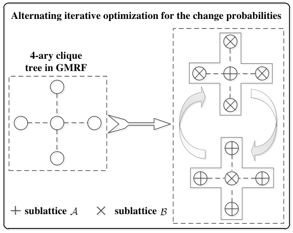
Therefore, an alternating iterative optimization scheme is developed to embed $L$ bits in cover image while minimizing the total KL-divergence by incorporating the proposed GMRF model as shown in Fig. 4. In specific, randomly initialize the $\bm{\beta}^{{\cal B}}$ in subimage ${\cal B}$ and keep them unchanged, solve (32) for $\bm{\beta}^{{\cal A}}$ in ${\cal A}$. Update the change probabilities for pixels in ${\cal A}$ with the newly obtained $\bm{\beta}^{{\cal A}}$ and then keep them unchanged, solve (34) for $\bm{\beta}^{{\cal B}}$ in ${\cal B}$. The process continues until it converges to obtain the optimal $\bm{\beta}^{{\cal A}}$ and $\bm{\beta}^{{\cal B}}$ for embedding payload of $L$ bits into cover image with minimum distortion. It is noted that: 1) the update of $\bm{\beta}^{{\cal A}}$ is affected somehow by the neighboring $\bm{\beta}^{{\cal B}}$ through the underlying GMRF model; 2) the problems specified in (32) and (34) are the ones of convex optimization, which are bound to converge to the globally optimal solutions. The readers are advised to refer to the pseudo-code (Algorithm 1) with practical consideration to better understand the process.

We then proceed to consider the practical issues in implementing the GMRF based image steganography. Recall that the interactions between neighboring pixels are explored by taking advantages of the proposed GMRF with four-element cross neighborhood, which doesn’t go well enough for embedding in rich texture regions of cover images. Fig. 5 shows a portion of image (1013.pgm) from BOSSbase [17], where the red boxes correspond to the texture regions and the black and white points inside images represent the ’$-$1’ and ’$+$1’ embeddings, respectively. The paradigm of adaptive image steganography encourages more data to be embedded in the texture regions of images by assigning low costs to changes to regions which exhibit less correlations among neighboring pixels. The red boxes in Fig. 5 (c) shows the embedding distribution using MiPOD [7] with a multivariate independent Gaussian model, which is appropriate to characterize the rich texture regions of images, while Fig. 5 (d) shows slightly sparser distributions in the same regions with the proposed GMRF, where all the four two-pixel cliques are included in the clique tree. This is because, for the two less correlated pixels in a clique, say, $X_{1}$ (low cost) and $X_{2}$ (high cost), the embedding cost for $X_{1}$ would increase during the alternating iterative optimization process, which may lead to less embeddings in the texture regions. Therefore, if two horizontally/vertically neighboring pixels are less correlated to some extents, the relevant clique should be disconnected from the GMRF model. Note that the correlation between two neighboring pixels is in connection with their variances, the involved two pixels are less correlated as long as one or two of them have relatively large variances. On the other hand, the ultimate goal for GMRF based optimization is to find the optimal change probability $\beta$ of each pixel $x$ in the cover image for minimum distortion embedding, while $\beta$ is directly proportional to pixel’s variance, thus the change probability $\beta$ can be used as an effective measure to dynamically allocate the relevant cliques in the alternating iterative optimization process, i.e., let ${{\bf{X}}_{c}}={[{X_{s}},{X_{t}}]^{T}}$ be the clique ${c}=\{{X_{s}},{X_{t}}\}$ ($t=1,..,4$) associated with the ${s^{th}}$ clique tree, we have

where $\theta_{c}^{T_{s}}$ is the statement to determine if clique ${{\bf{X}}_{c}}$ is included in the clique tree $T_{s}$, ${\beta_{T}}$ is the threshold, ${\beta_{X_{s}}}$ and ${\beta_{X_{t}}}$ are the change probabilities for the two pixels in clique ${{\bf{X}}_{c}}$, respectively. The introduction of (35) can then be regarded as the dynamical configuration of the initial neighborhood system ${\cal N}$ for GMRF based embedding with practical consideration. Fig. 5 (e) and (f) show the embedding distributions of GMRF in texture regions when the dynamical allocation scheme is applied and all the cliques are excluded in the clique trees, respectively. It is observed that the GMRF has denser embedding densities than MiPOD in red blocks, while shows similar densities with MiPOD in highly-textured regions. Note that the red blocks in Fig. 5 may consists of highly and medium textured regions, and the performance gains of the proposed GMRF over independent Gaussian model based schemes are mainly from the medium and less textured regions in images.

As a summary, we finally give the pseudo-code (Algorithm 1) for GMRF based embedding with practical consideration.

References

• [1] V. Holub and J. Fridrich, “Designing steganographic distortion using directional filters,” in Proc. IEEE Workshop on Information Forensic and Security, 2012, pp. 234–239.
• [2] V. Holub, J. Fridrich, and T. Denemark, “Universal distortion function for steganography in an arbitrary domain,” EURASIP Journal on Information Security, vol. 2014, no. 1, pp. 1–13, 2014.
• [3] B. Li, M. Wang, J. Huang, and X. Li, “A new cost function for spatial image steganography,” in Proc. IEEE International Conference on Image Processing, 2014, pp. 4206–4210.
• [4] J. Fridrich and J. Kodovský, “Multivariate gaussian model for designing additive distortion for steganography,” in Proc. IEEE International Conference on Acoustics, Speech and Signal Processing (ICASSP), 2013, pp. 2949–2953.
• [5] T. Pevný, T. Filler, and P. Bas, “Using high-dimensional image models to perform highly undetectable steganography,” in Bohme R., Fong P. W. L., Safavi-Naini R. (eds) Information Hiding, IH 2010, LNCS, vol. 6387, Springer, Calgary, AB, Canada, 2010, pp. 161–177.
• [6] V. Sedighi, J. Fridrich, , and R. Cogranne, “Content-adaptive pentary steganography using the multivariate generalized gaussian cover model,” in Proc. SPIE Electronic Imaging, Media Watermarking, Security, and Forensics, vol. 9409, 2015.
• [7] V. Sedighi, R. Cogranne, and J. Fridrich, “Content-adaptive steganography by minimizing statistical detectability,” IEEE Transactions on Information Forensics and Security, vol. 11, no. 2, pp. 221–234, 2016.
• [8] L. Guo, J. Ni, and Y. Q. Shi, “Uniform embedding for efficient JPEG steganography,” IEEE Transactions on Information Forensics and Security, vol. 9, no. 5, pp. 814–825, 2014.
• [9] L. Guo, J. Ni, W. Su, C. Tang, and Y. Q. Shi, “Using statistical image model for JPEG steganography: Uniform embedding revisited,” IEEE Transactions on Information Forensics and Security, vol. 10, no. 12, pp. 2669–2680, 2015.
• [10] W. Su, J. Ni, X. Li, and Y. Q. Shi, “A new distortion function design for jpeg steganography using the generalized uniform embedding strategy,” IEEE Transactions on Circuits and Systems for Video Technology, vol. 28, no. 12, pp. 3545–3549, 2018.
• [11] X. Hu, J. Ni, and Y. Q. Shi, “Efficient jpeg steganography using domain transformation of embedding entropy,” IEEE Signal Processing Letters, vol. 25, no. 6, pp. 773––777, 2018.
• [12] K. Chen, H. Zhou, W. Zhou, W. Zhang, and N. Yu, “Defining cost functions for adaptive jpeg steganography at the microscale,” IEEE Transactions on Information Forensics and Security, vol. 14, no. 4, pp. 1052–1066, 2019.
• [13] T. Filler, J. Judas, and J. Fridrich, “Minimizing additive distortion in steganography using syndrome-trellis codes,” IEEE Transactions on Information Forensics and Security, vol. 6, no. 3, pp. 920–935, 2011.
• [14] A. D. Ker, “Estimating steganographic fisher information in real images,” in Katzenbeisser S., Sadeghi AR. (eds) Information Hiding, IH2009, LNCS, vol. 5806, 2009, pp. 73–88.
• [15] J. Fridrich and J. Kodovský, “Rich models for steganalysis of digital images,” IEEE Transactions on Information Forensics and Security, vol. 7, no. 3, pp. 868–882, 2012.
• [16] T. Denemark, V. Sedighi, V. Holub, R. Cogranne, and J. Fridrich, “Selection-channel-aware rich model for steganalysis of digital images,” in Proc. IEEE International Workshop on Information Forensics and Security (WIFS), 2014, pp. 48–53.
• [17] P. Bas, T. Filler, and T. Pevný, “Break our steganographic system: the ins and outs of organizing BOSS,” in Filler T. and Pevný T.and Craver S. and Ker A.(eds) Information Hiding. IH 2011. LNCS, vol. 6958. Springer, Berlin, Heidelberg, 2011, pp. 59–70.
• [18] S. Z. Li, Markov Random Field Modeling in Image Analysis, 2nd ed. Springer London, 2009.
• [19] H. Rue and L. Held, Gaussian Markov Random Fields Theory and Applications. CRC, 2005.
• [20] J. E. Besag, “Spatial interaction and the statistical analysis of lattice systems,” Journal of the Royal Statistical Society, Series B (Methodological), vol. 36, no. 2, pp. 192–236, 1974.
• [21] [Online]. Available: http://fourier.eng.hmc.edu/e161/lectures/gaussianprocess/node7.html
• [22] T. Filler and J. Fridrich, “Fisher information determines capacity of epsilon-secure steganography,” in Katzenbeisser S., Sadeghi AR. (eds) Information Hiding, IH 2009, LNCS, vol. 5806. Springer, Darmstadt, Germany, 2009, pp. 31–47.
• [23] L. Isserlis, “On a formula for the product-moment coefficient of any order of a normal frequency distribution in any number of variables,” Biometrika, vol. 12, no. 1/2, pp. 134–139, 1918.
• [24] S. M. Kay, Fundamentals of Statistical Signal Processing, Volume I: Estimation Theory. Pearson Education, 1993.
• [25] V. Katkovnik, K. Egiazarian, and J. Astola, Local Approximation Techniques in Signal and Image Processing. SPIE Press, Monograph, 2006, vol. PM157.
• [26] L. F. Williams and Jr, “A modification to the half-interval search (binary search) method,” in Proceedings of the 14th Annual Southeast Regional Conference, 1976, pp. 95–101.
• [27] J. Kodovský, J. Fridrich, and V. Holub, “Ensemble classifiers for steganalysis of digital media,” IEEE Transactions on Information Forensics and Security, vol. 7, no. 2, pp. 432–444, 2012.
• [28] B. Li, S. Tan, M. Wang, and J. Huang, “Investigation on cost assignment in spatial image steganography,” IEEE Transactions on Information Forensics and Security, vol. 9, no. 8, pp. 1264–1277, 2014.