Minimum Energy Analysis for Robust Gaussian Joint Source-Channel Coding with a Square-Law Profile

Mohammadamin Baniasadi Ertem Tuncel Affiliation: Department of Electrical and Computer Engineering Affiliation: University of California, Riverside, CA Affiliation: Email: mohammadamin.baniasadi@email.ucr.edu, ertem.tuncel@ucr.edu

Abstract

A distortion-noise profile is a function indicating the maximum allowed source distortion value for each noise level in the channel. In this paper, the minimum energy required to achieve a distortion noise profile is studied for Gaussian sources which are transmitted robustly over Gaussian channels. We provide improved lower and upper bounds for the minimum energy behavior of the square-law profile using a family of lower bounds and our proposed coding scheme.

Index Terms–Distortion-noise profile, fidelity-quality profile, energy-distortion tradeoff, energy-limited transmission, joint source-channel coding.

I INTRODUCTION

Most of emerging wireless applications, such as Internet of things (IoT) and multimedia streaming require lossy transmission of source signals over noisy channels, which is in general a joint source-channel coding (JSSC) problem. Shannon proved the separation theorem which states that in point-to-point scenarios, it is optimal to separate source and channel coding problems. However, in many problems, the optimality of separation breaks down, since JSCC can exploit source correlation to generate correlated channel inputs despite the distributed nature of the encoders, potentially improving the overall performance [1]-[5].

We consider lossy transmission of a Gaussian source over an additive white Gaussian noise (AWGN) channel, where the channel input constraint is not on power and bandwidth, but on energy per source symbol. This approach has drawn much attention recently, see e.g., [6, 7, 8, 9] as a few references. Part of the appeal is the simplifications to both achievable schemes and converses as the bandwidth expansion factor approaches infinity [8]. We assume there is no feedback.

It is well-known (for example, see [6]) that the minimum distortion that can be achieved with energy $E$ when the channel noise variance $N$ is fixed, is given by

\displaystyle D=\exp(-\frac{E}{N}).

(1)

In this paper, a robust setting is considered in which the transmitter does not know $N$ , while it is known at the receiver, and it can have any value in the interval (0, $\infty$ ). The system is to be designed to fulfill with a distortion-noise profile ${\cal D}(N)$ so that it achieves

\displaystyle D\leq\mathcal{D}(N)

for all $0<N<\infty$ , while minimizing its energy use. This wide spectrum of noise variances is taken into consideration to account for the scenarios in which absolutely nothing is known about the noise level. For instance, the channel could be suffering occasional interferences of unknown power ( $N>0$ ), although it may be originally of very high quality ( $N\approx 0$ ). There are a wide range of applications in which noise variances are not known. For instance, we can point military situation, indoor fires and emergency conditions.

In [10], it is shown that for the inversely linear profile, uncoded transmission is optimal. Furthermore,it is represented that exponential profiles are not achievable with finite energy. Then, the square-law profile is studied which is somehow combination of linear and exponential profiles and lower and upper bounds have been derived for the minimum achievable energy of the square-law profile. In this paper, we derive improved lower and upper bounds for the minimum energy, and show that the gap between our lower and upper bounds is significantly reduced compared to [10]. Improving lower and upper bounds and making them as tight as possible helps us to design better systems in practical scenarios by comparing the amount of energy with these improved theoretical bounds.

A similar universal coding scenario in the literature is given in [11], where a maximum regret approach for compound channels is proposed. The objective in their problem is to minimize the maximum ratio of the capacity to the achieved rate at any noise level. There are other related works including [12, 13], and [14].

The rest of the paper is organized as follows. The next section is devoted to notation and preliminaries. In Section III, previous work on lower and upper bounds for the minimum energy is reviewed. In Section IV, we present our main results, which are improved lower and upper bounds for the square-law profile. Finally, in Section V we conclude our work and discuss future work.

II Notation and Preliminaries

Suppose that $X^{n}$ is an i.i.d unit-variance Gaussian source which is transmitted over an AWGN channel $V^{m}=U^{m}+W^{m}$ , where $U^{m}$ is the channel input, $W^{m}\sim\mathcal{N}(\mathbf{0},N\mathbf{I}_{m})$ is the noise, and $V^{m}$ is the observation at the receiver. We define bandwidth expansion factor $\kappa=\frac{m}{n}$ which can be arbitrarily large, while the energy per source symbol is limited by

\displaystyle\frac{1}{n}E(||U^{m}||^{2})\leq E.

(2)

The achieved distortion per source symbol is measured as

\displaystyle D=\frac{1}{n}E(||X^{n}-\hat{X}^{n}||^{2})

(3)

while $\hat{X}^{n}$ is the reconstruction at the receiver.

Definition 1

A pair of distortion-noise profile $\mathcal{D}(N)$ and energy level $E$ is said to be achievable if for every $\epsilon>0$ , there exists large enough $(m,n)$ , an encoder

\displaystyle f^{m,n}:R^{n}\to R^{m},

and decoders

\displaystyle g_{N}^{m,n}:R^{m}\to R^{n}

for every $0<N<\infty$ , such that

\displaystyle\frac{1}{n}E\{||f^{m,n}(X^{n})||^{2}\}\leq E+\epsilon

and

\displaystyle\frac{1}{n}E\{||X^{n}-g_{N}^{m,n}(f^{m,n}(X^{n})+W_{N}^{m})||^{2}\}\leq\mathcal{D}(N)+\epsilon

for all $N$ , with $W_{N}^{m}$ being the i.i.d. channel noise with variance $N$ .

For given $\mathcal{D}$ , the main quantity of interest would be

\displaystyle E_{min}(\mathcal{D})=\inf\{E:(\mathcal{D},E)\ \textrm{achievable}\}

with the understanding that $E_{min}(\mathcal{D})=\infty$ if there is no finite $E$ for which $(\mathcal{D},E)$ is achievable.

In the sequel, it will prove more convenient to use the notation $F=\frac{1}{D}$ and $Q=\frac{1}{N}$ , where $F$ and $Q$ standing for signal fidelity and channel quality, respectively as in [10]. For any $\mathcal{D}(N)$ , we define the corresponding fidelity-quality profile as

\displaystyle\mathcal{F}(Q)=\frac{1}{\mathcal{D}(\frac{1}{Q})}

and state that $(\mathcal{F},E)$ is achievable if and only if $(\mathcal{D},E)$ is achievable according to Definition 1. $E_{min}(\mathcal{F})$ is similarly defined.

III Previous Work

III-A A Family of Lower Bounds on $E_{min}(\mathcal{D})$

In [10], the authors used the connection between the problem and lossy transmission of Gaussian sources over Gaussian broadcast channels where the power per channel symbol is limited and the bandwidth expansion factor $\kappa$ is fixed. More specifically, they employed the converse result by Tian et al. [15], which is a generalization of the 2-receiver outer bound shown by Reznic et al. [16] to $K$ receivers, and proved the following lemma.

Lemma 1

For any $K$ , $\tau_{1}\geq\tau_{2}\geq...\geq\tau_{K-1}\geq\tau_{K}=0$ , and $N_{1}\geq N_{2}\geq...\geq N_{K}\geq N_{K+1}=0$ ,

	$\displaystyle E_{min}(\mathcal{D})\!\!\!$	$\displaystyle\geq$	$\displaystyle\!\!\!N_{1}\log\frac{1+\tau_{1}}{\mathcal{D}(N_{1})+\tau_{1}}$		(4)
			$\displaystyle\!\!\!+\sum_{k=2}^{K}N_{k}\log\frac{(1+\tau_{k})(\mathcal{D}(N_{k})+\tau_{k-1})}{(1+\tau_{k-1})(\mathcal{D}(N_{k})+\tau_{k})}.$		(4)

III-B Square-Law Fidelity Quality Profiles

In [10], the authors focused on $\mathcal{F}(Q)=1+\alpha Q^{2}$ for some $\alpha>0$ and analyzed the lower and upper bounds for $E_{min}{(\mathcal{F})}$ .

III-B1 Lower Bound for $E_{min}(\mathcal{F})$

Invoking Lemma 1 by properly choosing $\tau_{k}$ and $N_{k}$ in (4), the following theorem was obtained in [10].

Theorem 1

For a fidelity-quality profile $\mathcal{F}(Q)=1+\alpha Q^{2}$ , the minimum required energy is lower-bounded as

\displaystyle E_{min}(\mathcal{F})\geq c\ \sqrt{\alpha}

with

\displaystyle c=\sum_{k=1}^{\infty}\frac{1}{\sqrt{4^{k}\exp(k)-1}}\approx 0.4507.

III-B2 Upper Bound for $E_{min}(\mathcal{F})$

Using a scheme first sending the source uncoded, and leveraging the received output as side information for the subsequent digital rounds sending indices of an infinite-layer quantizer, an upper bound for the minimum energy was presented in the following theorem in [10].

Theorem 2

The minimum required energy for profile $\mathcal{F}(Q)=1+\alpha Q^{2}$ is upper-bounded as

\displaystyle E_{min}(\mathcal{F})\leq d\ \sqrt{\alpha}

with

\displaystyle d=2\ \sqrt{\log 3-Li_{2}(-2)}\approx 3.1846

where $Li_{2}(.)$ is the polylogarithm of order 2 defined as

\displaystyle Li_{2}(z)=-\int_{0}^{1}\frac{\log(1-zu)}{u}du.

IV Our Main Results

Our main contributions in this paper are tighter lower and upper bounds to the energy for the profile ${\cal F}(Q)=1+\alpha Q^{2}$ .

IV-A Lower Bound for $E_{min}(\mathcal{F})$

We begin with lower bounding $E_{\min}({\cal F})$ by the following theorem.

Theorem 3

For a fidelity-quality profile ${\cal F}(Q)=1+\alpha Q^{2}$ , the minimum required energy is lower-bounded as

E_{\min}({\cal F})\geq 0.9057\sqrt{\alpha}.

Proof:

A lower bound on $E_{min}(\mathcal{D})$ follows from (1). Since for any fixed $N_{0}$ and $D_{0}$ the expended energy cannot be lower than $N_{0}\log\frac{1}{D_{0}}$ , the lower bound is obtained given by

\displaystyle E_{min}(\mathcal{D})\geq\sup_{N>0}N\log\frac{1}{\mathcal{D}(N)}

(5)

or equivalently by

$\displaystyle E_{min}(\mathcal{F})$	$\displaystyle\geq\sup_{Q>0}\frac{\log\mathcal{F}(Q)}{Q}$
	$\displaystyle=\sup_{Q>0}\frac{\log(1+\alpha Q^{2})}{Q}$
	$\displaystyle=\bigg(\sup_{q>0}\frac{\log(1+q^{2})}{q}\bigg)\sqrt{\alpha}$	(6)

where $q=\sqrt{\alpha}Q$ . By solving (IV-A) numerically, optimal value of $q$ is $q^{*}=2.01$ and thus

\displaystyle E_{min}(\mathcal{F})\geq 0.8047\sqrt{\alpha}.

(7)

Note that (IV-A) is the special case of Lemma 1 where $K=1$ . Thus, it is reasonable to expect an even better lower bound by increasing $K$ . By setting $K=2$ and $\tau_{1}=\tau\geq\tau_{2}=0$ , the lower bound is achieved as

	$\displaystyle E_{min}(\mathcal{F})$	$\displaystyle\geq\sup_{Q_{2}>Q_{1}>0,\tau>0}\Bigg[\frac{\log(1+\frac{\alpha Q^{2}_{1}}{1+\tau(1+\alpha Q^{2}_{1})})}{Q_{1}}+\frac{\log(1+\frac{\alpha\tau Q^{2}_{2}}{1+\tau})}{Q_{2}}\Bigg]$
		$\displaystyle\geq\Bigg(\sup_{q_{2}>q_{1}>0,\tau>0}\bigg[\frac{\log(1+\frac{q^{2}_{1}}{1+\tau(1+q^{2}_{1})})}{q_{1}}+\frac{\log(1+\frac{\tau q^{2}_{2}}{1+\tau})}{q_{2}}\bigg]\Bigg)\sqrt{\alpha}$		(8)

where $q_{1}=\sqrt{\alpha}Q_{1}$ and $q_{2}=\sqrt{\alpha}Q_{2}$ , respectively.

In order to compute the supremum in (IV-A), we use the gradient ascent algorithm. As the initial point, we set $q_{1}=2.01$ and $\tau=0$ which give us the same lower bound (7) for any arbitrary choice of $q_{2}$ . Starting from this initial point (together with the arbitrary choice $q_{2}=3$ ), the algorithm converged to $q^{*}_{1}=1.5496$ , $q^{*}_{2}=5.6679$ , $\tau^{*}=0.1285$ , and the corresponding lower bound is achieved as

\displaystyle E_{min}(\mathcal{F})\geq 0.9057\sqrt{\alpha}.

(9)

∎Comparing Theorem 1 with Theorem 3 shows that the lower bound is tightened significantly.

IV-B Upper Bound for $E_{min}(\mathcal{F})$

To upper bound $E_{min}(\mathcal{F})$ , we introduce a $K$ -layer coding scheme which has a $K$ -layer quantizer and sends the quantization indices using Wyner-Ziv coding, where the $k$ th quantization index is to be decoded whenever $N\leq N_{k}$ for some predetermined $N_{1}\geq N_{2}\geq\ldots\geq N_{K}$ . However, instead of relying on only one uncoded transmission of the source $X^{n}$ as the generator of the side information at the receiver, we also send quantization errors uncoded after each layer of quantization. In other words, we have $K$ layers of uncoded transmission while in [10] the authors only had the uncoded transmission in first layer.

It is not immediately obvious that this strategy will reduce the total expended energy, because even though the energy needed to convey quantization indices will be reduced because of a richer set of available side information, transmission of the quantization errors themselves consumes additional energy. However, as we show here, the minimum energy needed is indeed reduced compared to the scheme in [10].

TABLE I: Utilization of information in our proposed coding scheme

Noise interval	$N>N_{1}$	$N_{1}\geq N>N_{2}$	$N_{2}\geq N>N_{3}$	$...$	$N_{K}\geq N>N_{K+1}$
Decoded digital information
	$-$	$\hat{S}^{n}_{1}$	$\hat{S}^{n}_{1}$		$\hat{S}^{n}_{1}$
			$\hat{S}^{n}_{2}$		.
				$...$	.
					.
					$\hat{S}^{n}_{K}$
Effective side information
	$\sqrt{A_{0}}S^{n}_{0}+W^{n}_{0,N}$	$\sqrt{A_{0}}S^{n}_{1}+W^{n}_{0,N}$	$\sqrt{A_{0}}S^{n}_{2}+W^{n}_{0,N}$		$\sqrt{A_{0}}S^{n}_{K}+W^{n}_{0,N}$
		$\sqrt{A_{1}}S^{n}_{1}+W^{n}_{1,N}$	$\sqrt{A_{1}}S^{n}_{2}+W^{n}_{1,N}$		.
			$\sqrt{A_{2}}S^{n}_{2}+W^{n}_{2,N}$		.
				$...$	.
					.
					.
					$\sqrt{A_{K}}S^{n}_{K}+W^{n}_{K,N}$

The source $X^{n}$ is successively quantized into source codewords $\hat{S}^{n}_{k}$ for $k=1,\ldots,K$ , where the underlying single-letter characterization satisfies

\displaystyle S_{k}=\hat{S}_{k+1}+S_{k+1}

with $S_{0}=X$ and $\hat{S}_{k+1}\perp S_{k+1}$ . Each $S_{k}^{n}$ for $k=0,1,\ldots,K$ is then sent in an uncoded fashion, i.e., as $\sqrt{A_{k}}S_{k}^{n}$ . For any noise variance $0<N<\infty$ , the received signals will then be given by

Y^{n}_{i,N}=\sqrt{A_{i}}S_{i}^{n}+W^{n}_{i,N}

for $i=0,\ldots,K$ . When $N>N_{1}$ , the $X^{n}$ will be estimated only by utilizing $Y^{n}_{0,N}$ . On the other hand, when $N_{k+1}<N\leq N_{k}$ , for $k=1,2,\ldots,K$ , since the first $k$ layers of quantization indices will already be decoded, the estimation can rely on all

\displaystyle\tilde{Y}^{n}_{i,N}=\sqrt{A_{i}}S^{n}_{k}+W^{n}_{i,N}

as effective side information, as all $\hat{S}^{n}_{i}$ for $i=1,...,k$ can be subtracted from $X^{n}$ . The utilization of information in our coding scheme is summarized in TABLE I.

Now, to be able to decode $\hat{S_{k}}$ whenever $N\leq N_{k}$ , it suffices to use a binning rate of

$\displaystyle R_{k}$	$\displaystyle=$	$\displaystyle I(S_{k-1};\hat{S}_{k}\|\tilde{Y}_{0,N_{k}},\tilde{Y}_{1,N_{k}},...,\tilde{Y}_{k-1,N_{k}})$	(10)
	$\displaystyle=$	$\displaystyle I(S_{k-1};\hat{S}_{k})-I(\tilde{Y}_{0,N_{k}},\tilde{Y}_{1,N_{k}},...,\tilde{Y}_{k-1,N_{k}};\hat{S}_{k})$
	$\displaystyle=$	$\displaystyle h(S_{k-1})-h(S_{k})$
		$\displaystyle-h(\tilde{Y}_{0,N_{k}},\tilde{Y}_{1,N_{k}},...,\tilde{Y}_{k-1,N_{k}})$
		$\displaystyle+h(\tilde{Y}_{0,N_{k}},\tilde{Y}_{1,N_{k}},...,\tilde{Y}_{k-1,N_{k}}\|\hat{S}_{k})$
	$\displaystyle=$	$\displaystyle\frac{1}{2}\log\frac{\sigma^{2}_{S_{k-1}}}{\sigma^{2}_{S_{k}}}-\frac{1}{2}\log\frac{\det\mathbf{\Sigma}_{\mathbf{Y}_{k}}}{\det\mathbf{\Sigma}_{\mathbf{Y}_{k}\|\hat{S}_{k}}}$

where

\mathbf{\Sigma}_{\mathbf{Y}_{k}}=\mathbf{A}_{k}\mathbf{\Sigma}_{\mathbf{Z}_{k}}\mathbf{A}_{k}^{T}

with

\displaystyle\mathbf{A}_{k}=\begin{bmatrix}\sqrt{A_{0}}&1&0&0&.&.&.&0\\ \sqrt{A_{1}}&0&1&0&.&.&.&0\\ .&.&.&1&.&.&.&0\\ .&.&.&.&1&.&.&0\\ .&.&.&.&.&1&.&0\\ \sqrt{A_{k-1}}&0&0&0&.&.&.&1\\ \end{bmatrix}

and

\displaystyle\mathbf{Z}_{k}=\begin{bmatrix}S_{k-1}\\ W_{0,N_{k}}\\ W_{1,N_{k}}\\ \vdots\\ W_{k-1,N_{k}}\end{bmatrix}\;.

Similarly,

\mathbf{\Sigma}_{\mathbf{Y}_{k}|\hat{S}_{k}}=\mathbf{A}_{k}\mathbf{\Sigma}_{\mathbf{\tilde{Z}}_{k}}\mathbf{A}_{k}^{T}

with

\displaystyle\mathbf{\tilde{Z}}_{k}=\begin{bmatrix}S_{k}\\ W_{0,N_{k}}\\ W_{1,N_{k}}\\ \vdots\\ W_{k-1,N_{k}}\end{bmatrix}\;.

Since the source and channel noise are independent, both $\mathbf{\Sigma}_{\mathbf{Z}_{k}}$ and $\mathbf{\Sigma}_{\mathbf{\tilde{Z}}_{k}}$ are diagonal, and that makes the computation of $\mathbf{\Sigma}_{\mathbf{Y}_{k}}$ and $\mathbf{\Sigma}_{\mathbf{Y}_{k}|\hat{S}_{k}}$ easy. Specifically, defining the $k\times k$ matrix

\mathbf{G}_{k}=\begin{bmatrix}1&0&.&.&.&0\\ 0&0&0&.&.&0\\ .&0&0&0&.&0\\ .&.&0&.&0&0\\ .&.&.&.&0&0\\ 0&0&0&0&0&0\\ \end{bmatrix},

one can write

\mathbf{\Sigma}_{\mathbf{Z}_{k}}=N_{k}\mathbf{I}_{k}+(\sigma^{2}_{S_{k-1}}-N_{k})\mathbf{G}_{k}\;.

and

\mathbf{\Sigma}_{\mathbf{\tilde{Z}}_{k}}=N_{k}\mathbf{I}_{k}+(\sigma^{2}_{S_{k}}-N_{k})\mathbf{G}_{k}\;.

We then have

$\displaystyle\mathbf{\Sigma}_{\mathbf{Y}_{k}}$	$\displaystyle=\mathbf{A}_{k}\bigg(N_{k}\mathbf{I}_{k}+(\sigma^{2}_{S_{k-1}}-N_{k})\mathbf{G}_{k}\bigg)\mathbf{A}_{k}^{T}$
	$\displaystyle=N_{k}\mathbf{A}_{k}\mathbf{I}_{k}\mathbf{A}_{k}^{T}+(\sigma^{2}_{S_{k-1}}-N_{k})\mathbf{A}_{k}\mathbf{G}_{k}\mathbf{A}_{k}^{T}$
	$\displaystyle=N_{k}\mathbf{A}_{k}\mathbf{A}_{k}^{T}+(\sigma^{2}_{S_{k-1}}-N_{k})\mathbf{a}_{k}\mathbf{a}_{k}^{T}$
	$\displaystyle=N_{k}(\mathbf{a}_{k}\mathbf{a}_{k}^{T}+\mathbf{I}_{k})+(\sigma^{2}_{S_{k-1}}-N_{k})\mathbf{a}_{k}\mathbf{a}_{k}^{T}$
	$\displaystyle=N_{k}\mathbf{I}_{k}+\sigma^{2}_{S_{k-1}}\mathbf{a}_{k}\mathbf{a}_{k}^{T}\;$	(11)

where $\mathbf{a}_{k}$ is the first column of matrix $\mathbf{A}_{k}$ . Similarly,

\displaystyle\mathbf{\Sigma}_{\mathbf{Y}_{k}|\hat{S}_{k}}=N_{k}\mathbf{I}_{k}+\sigma^{2}_{S_{k}}\mathbf{a}_{k}\mathbf{a}_{k}^{T}.

(12)

By substituting (11) and (12) in (10), we then get

\displaystyle R_{k}=\frac{1}{2}\log\frac{\sigma^{2}_{S_{k-1}}}{\sigma^{2}_{S_{k}}}-\frac{1}{2}\log\frac{\det(N_{k}\mathbf{I}_{k}+\sigma^{2}_{S_{k-1}}\mathbf{a}_{k}\mathbf{a}_{k}^{T})}{\det(N_{k}\mathbf{I}_{k}+\sigma^{2}_{S_{k}}\mathbf{a}_{k}\mathbf{a}_{k}^{T})}.

(13)

Using the Matrix Determinant Lemma [17], which states for arbitrary invertible $\mathbf{M}$ and column vectors $\mathbf{u}$ and $\mathbf{v}$ that

\det(\mathbf{M}+\mathbf{u}\mathbf{v}^{T})=\det(\mathbf{M})\cdot(1+\mathbf{v}^{T}\mathbf{M}^{-1}\mathbf{u})

We can write

$\displaystyle R_{k}$	$\displaystyle=\frac{1}{2}\log\frac{\sigma^{2}_{S_{k-1}}}{\sigma^{2}_{S_{k}}}-\frac{1}{2}\log\frac{(1+\frac{\sigma^{2}_{S_{k-1}}}{N_{k}}\mathbf{a}_{k}^{T}\mathbf{a}_{k})}{(1+\frac{\sigma^{2}_{S_{k}}}{N_{k}}\mathbf{a}_{k}^{T}\mathbf{a}_{k})}$
	$\displaystyle=\frac{1}{2}\log\frac{\sigma^{2}_{S_{k-1}}(1+\frac{\sigma^{2}_{S_{k}}}{N_{k}}\mathbf{a}_{k}^{T}\mathbf{a}_{k})}{\sigma^{2}_{S_{k}}(1+\frac{\sigma^{2}_{S_{k-1}}}{N_{k}}\mathbf{a}_{k}^{T}\mathbf{a}_{k})}$
	$\displaystyle=\frac{1}{2}\log\frac{\beta_{k}+Q_{k}A_{k,\rm{total}}}{\beta_{k-1}+Q_{k}A_{k,\rm{total}}}$	(14)

where $\beta_{k}=\frac{1}{\sigma^{2}_{S_{k}}}$ , $Q_{k}=\frac{1}{N_{k}}$ , and

A_{k,\rm{total}}\stackrel{{\scriptstyle\Delta}}{{=}}A_{0}+A_{1}+...+A_{k-1}\;.

For the digital message, we use the channel with infinite bandwidth and energy $B_{k}$ . Therefore, the rate must not exceed the channel capacity under the noise level $N_{k}$ , i.e.,

\frac{1}{2}\log\frac{\beta_{k}+Q_{k}A_{k,\rm{total}}}{\beta_{k-1}+Q_{k}A_{k,\rm{total}}}\leq C_{k}=\frac{B_{k}Q_{k}}{2}

or equivalently,

\frac{\beta_{k}+Q_{k}A_{k,\rm{total}}}{\beta_{k-1}+Q_{k}A_{k,\rm{total}}}\leq\exp(B_{k}Q_{k})\;.

When $N_{k+1}<N\leq N_{k}$ , or equivalently when $Q_{k}\leq Q<Q_{k+1}$ , the MMSE estimation boils down to estimating $\tilde{S}_{k}^{n}$ using all the available effective side information, that is

\tilde{S}_{k}^{n}=\sum_{i=0}^{k}\lambda_{i}\tilde{Y}_{i,N}

with appropriate $\lambda_{i}$ for $i=0,1,\ldots,k$ . Thus, the resultant distortion can be calculated with the help of the Sherman-Morrison-Woodbury identity [17] as

$\displaystyle D$	$\displaystyle=\sigma^{2}_{S_{k}}-(\sigma^{2}_{S_{k}})^{2}\mathbf{a}_{k+1}^{T}\left(N\mathbf{I}_{k+1}+\sigma^{2}_{S_{k}}\mathbf{a}_{k+1}\mathbf{a}_{k+1}^{T}\right)^{-1}\mathbf{a}_{k+1}$
	$\displaystyle=\sigma^{2}_{S_{k}}-(\sigma^{2}_{S_{k}})^{2}\mathbf{a}_{k+1}^{T}\left[Q\mathbf{I}_{k+1}-\frac{Q^{2}\mathbf{a}_{k+1}\mathbf{a}_{k+1}^{T}}{\beta_{k}+Q\mathbf{a}_{k+1}^{T}\mathbf{a}_{k+1}}\right]\mathbf{a}_{k+1}$
	$\displaystyle=\sigma^{2}_{S_{k}}-(\sigma^{2}_{S_{k}})^{2}QA_{k+1,\rm{total}}\left[1-\frac{QA_{k+1,\rm{total}}}{\beta_{k}+QA_{k+1,\rm{total}}}\right]$
	$\displaystyle=\sigma^{2}_{S_{k}}-\sigma^{2}_{S_{k}}QA_{k+1,\rm{total}}\left[\frac{1}{\beta_{k}+QA_{k+1,\rm{total}}}\right]$
	$\displaystyle=\frac{1}{\beta_{k}+QA_{k+1,\rm{total}}}.$	(15)

Equivalently, the fidelity can be written as

\displaystyle F(Q)=\beta_{k}+QA_{k+1,\rm{total}}\;.

(16)

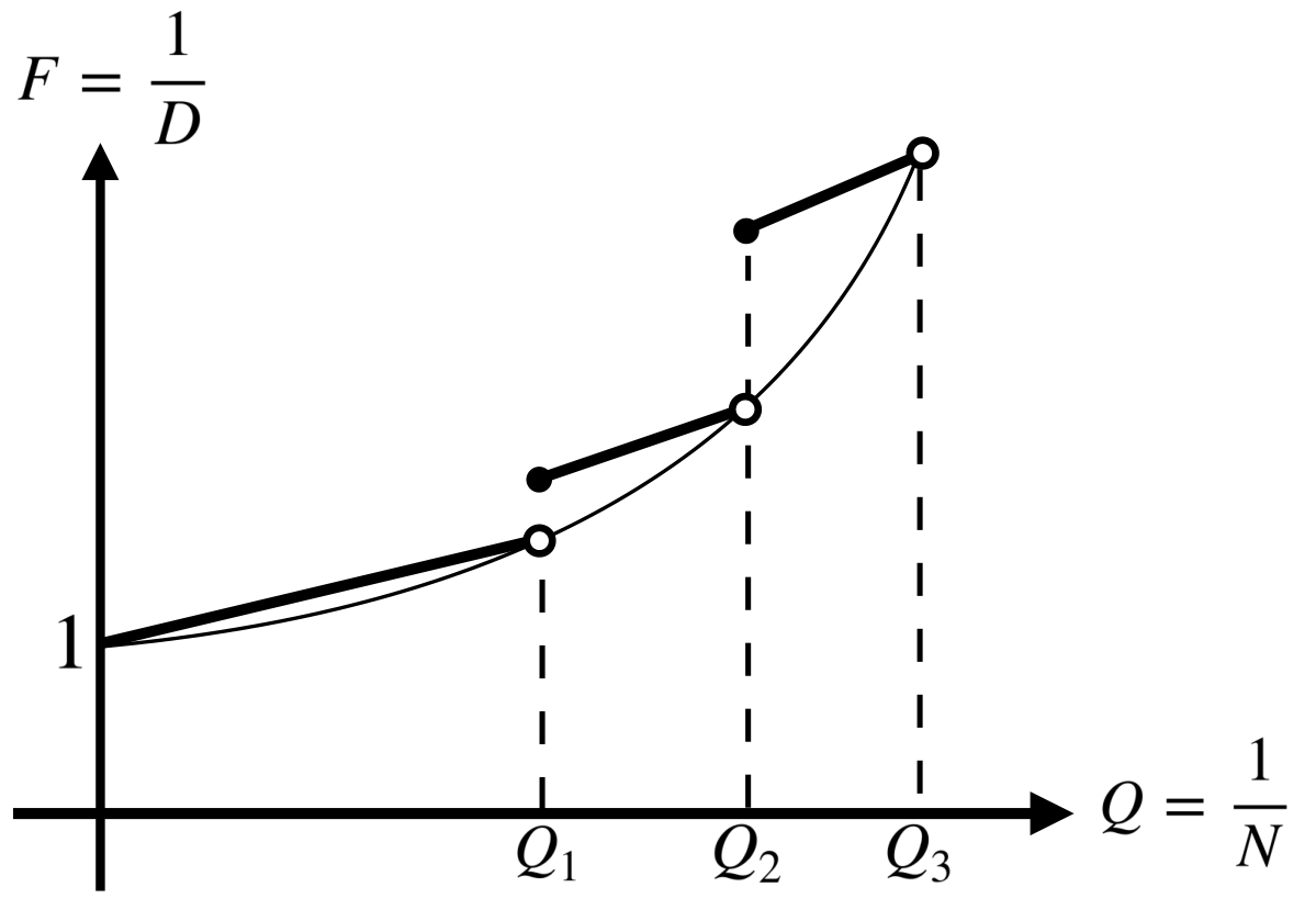
Therefore, $F(Q)$ is an “inclined” staircase function with changing slope $A_{k+1,\rm{total}}$ within each $Q_{k}\leq Q<Q_{k+1}$ as shown in Fig. 1. The beauty of the work is that we deal with linear segments. Thus, our analysis is easily understandable. Please note that Fig. 1 is different with the figure presented in [10]. The slope of inclined staircase function is fixed and equal to $E_{0}$ in [10], which is a special case of our work by letting $A_{0}=E_{0}$ and $A_{i}=0$ for $i=1,2,...$ . We are now ready to propose an upper bound on $E_{min}({\cal F})$ .

Refer to caption — Fig. 1: The fidelity-quality tradeoff is always above the profile $F(Q)$ , coinciding with it at the jump points $Q_{k}$ .

Theorem 4

The minimum required energy for profile $F(Q)=1+\alpha Q^{2}$ is upper-bounded as

\displaystyle E_{min}(F)\leq e\ \sqrt{\alpha}

with $e\approx 2.3203$ .

Proof:

We will use the scheme described above such that for any $0=Q_{0}<Q_{1}<Q_{2}<...,$ the energy $A_{k}$ and the source coding parameters $1=\beta_{0}<\beta_{1}<\beta_{2}<...$ will be chosen such that the fidelity-quality tradeoff in (16) is always above the profile $F(Q)$ , coinciding with it at the jump points $Q_{k}$ , as shown in Fig. 1. In other words,

\displaystyle A_{k,\rm{total}}Q_{k}+\beta_{k-1}=1+\alpha Q^{2}_{k}

(17)

for all $k=1,2,...$ .

Thus, we obtain

	$\displaystyle\beta_{k-1}$	$\displaystyle=1+\alpha Q^{2}_{k}-A_{k,\rm{total}}Q_{k}$
		$\displaystyle=1+\alpha Q^{2}_{k}-(A_{0}+A_{1}+...+A_{k-1})Q_{k}.$		(18)

The requirement that $\beta_{k}$ is increasing in $k$ leads to the following constraint

	$\displaystyle A_{0}$	$\displaystyle=\alpha Q_{1}$
	$\displaystyle A_{k}$	$\displaystyle<\frac{\alpha(Q^{2}_{k+1}-Q^{2}_{k})-A_{k,\rm{total}}(Q_{k+1}-Q_{k})}{Q_{k+1}},$		(19)

for all $k\geq 1$ .

Lemma 2

For fixed $\alpha$ , the choice $Q_{k}=k\Delta$ , $A_{0}=\alpha\Delta$ and $A_{k}=d^{k}\alpha\Delta$ for $k\geq 1$ satisfies (IV-B) for any $0<d<1$ and $\Delta>0$ .

Proof:

Substituting $A_{k}$ and $Q_{k}$ in (IV-B) yields:

\displaystyle d^{k}<\frac{(2k+1)-(\frac{d^{k}-1}{d-1})}{k+1}.

(20)

We use induction to prove (20). For $k=1$ , (20) reduces to $d<1$ which is true. Substituting $k=l$ , we get to the following:

\displaystyle d^{l}(l+1)<(2l+1)-(d^{l-1}+...+d+1)

(21)

We assume (21) is true. Now we substitute $k=l+1$ in (20) and have the following:

\displaystyle d^{l+1}(l+2)<(2l+3)-(d^{l}+d^{l-1}+...+d+1).

(22)

In order to complete the proof, we show (22) is true as follows. First, we multiply both sides of (21) with $d$ and then add $d^{l+1}$ to both sides, yielding

\displaystyle d^{l+1}(l+2)<(2l+1)d+d^{l+1}-(d^{l}+...+d).

(23)

Now, it suffices to show the right hand side of (23) is less than or equal to the right hand side of (22), which is the same as

\displaystyle d^{l+1}+(2l+1)d\leq 2l+2.

(24)

Since $0<d<1$ , we have $(2l+1)d<(2l+1)$ and $d^{l+1}<1$ . Thus, (24) is valid and the proof of Lemma 2 is complete. ∎ By substituting $A_{k}$ and $Q_{k}$ in (IV-B), we get

\displaystyle\beta_{k-1}

\displaystyle=1+\alpha k^{2}\Delta^{2}-k\alpha\Delta^{2}\bigg(\frac{1-d^{k}}{1-d}\bigg).

Letting $K\to\infty$ , the total uncoded energy becomes

	$\displaystyle E_{unc}$	$\displaystyle=\sum_{k=0}^{\infty}\frac{A_{k}}{\beta_{k}}$
		$\displaystyle=\sum_{k=0}^{\infty}\frac{d^{k}\alpha\Delta}{1+\alpha(k+1)^{2}\Delta^{2}-(k+1)\alpha\Delta^{2}\bigg(\frac{1-d^{k+1}}{1-d}\bigg)}.$		(25)

TABLE II: Comparison between our lower and upper bounds with the bounds in [10]

	1	10	100	1000	10000
Lower bound of [10]	0.4507	1.4252	4.5070	14.2524	45.0700
Our lower bound	0.9057	2.8641	9.0570	28.6407	90.5700
Upper bound of [10]	3.1846	10.0706	31.8460	100.7059	318.4600
Our upper bound	2.3203	7.3374	23.2030	73.3743	232.0300
The lower bound improvement	0.4550	1.4388	4.5500	14.3884	45.5000
The upper bound improvement	0.8643	2.7332	8.6430	27.3316	86.4300

On the other hand, the total digital energy is

$\displaystyle E_{dig}$	$\displaystyle=\sum_{k=1}^{\infty}B_{k}$
	$\displaystyle=\sum_{k=1}^{\infty}\frac{1}{Q_{k}}\log\Bigg(1+\frac{\beta_{k}-\beta_{k-1}}{1+\alpha Q^{2}_{k}}\Bigg)$
	$\displaystyle=\sum_{k=1}^{\infty}\frac{1}{k\Delta}\log\Bigg(1+\frac{\alpha\Delta^{2}\bigg(2k+1-kd^{k}-(\frac{1-d^{k+1}}{1-d})\bigg)}{1+\alpha k^{2}\Delta^{2}}\Bigg).$	(26)

Denoting $\Delta=\frac{c}{\sqrt{\alpha}}$ , we then get

		$\displaystyle E_{total}=E_{unc}+E_{dig}$
		$\displaystyle\leq\sqrt{\alpha}\sum_{k=0}^{\infty}\frac{cd^{k}}{1+c^{2}(k+1)^{2}-(k+1)c^{2}\bigg(\frac{1-d^{k+1}}{1-d}\bigg)}$
		$\displaystyle+\sqrt{\alpha}\sum_{k=1}^{\infty}\frac{1}{kc}\log\Bigg(1+\frac{c^{2}\bigg(2k+1-kd^{k}-(\frac{1-d^{k+1}}{1-d})\bigg)}{1+k^{2}c^{2}}\Bigg).$		(27)

In order to minimize the upper bound on total energy, we solve (IV-B) numerically for different values of $c$ and $d$ . For optimal values $d^{*}=0.999$ and $c^{*}=0.00137$ , the upper bound yields

\displaystyle E_{total}\leq 2.3203\sqrt{\alpha}.

∎

Comparing Theorem 2 with Theorem 4, we notice that the upper bound is improved significantly. Note that by setting $d=0$ and $A_{0}=E_{0}$ in our work, the method in [10] is achieved exactly. This is expected, as [10] is a special case of our work.

We compare our lower and upper bounds with the bounds in [10] for some values of $\alpha$ and show our improvements in TABLE 2.

V Conclusions and Future Work

Minimum energy required to achieve a distortion-noise profile, i.e., a function indicating the maximum allowed distortion value for each noise level, is studied for robust transmission of Gaussian sources over Gaussian channels. In order to analyze the minimum energy behavior for the square-law distortion noise profile, the lower and upper bounds were proposed by our coding scheme. We improved both upper and lower bounds significantly. For future, we are interested to study the distortion-noise profile problem in Multiple Access Channels (MAC). In MAC, instead of having one distortion function, we deal with at least two distortion functions and distortion regions.

References

[1] A. Lapidoth and S. Tinguely, “Sending a bivariate Gaussian over a Gaussian MAC,” IEEE Transactions on Information Theory, vol. 56, no. 6, pp. 2714 - 2752, Jun. 2010.
[2] P. Minero, S. Lim, and Y.-H. Kim, “Joint source-channel coding via hybrid coding,” IEEE International Symposium on Information Theory Proceedings (ISIT), pp. 781-785, Jul. 2011.
[3] W. Liu and B. Chen, “Interference channels with arbitrarily correlated sources,” IEEE Transactions on Information Theory, vol. 57, no. 12, pp. 8027-8037, Dec. 2011.
[4] M. P. Wilson, K. Narayanan, and G. Caire, “Joint source channel coding with side information using hybrid digital analog codes,” IEEE Transactions on Information Theory, vol. 56, no. 10, pp. 4922–4940, Oct. 2010.
[5] I. Estella and D. Gunduz, “Hybrid digital-analog transmission for the Gaussian one-helper problem,” IEEE Global Telecommunications Conference (GLOBECOM 2010), pp. 1 -5, Dec. 2010.
[6] A. Jain, D. Gunduz, S. R. Kulkarni, H. V. Poor, and S. Verdú, “Energy-distortion tradeoffs in Gaussian joint source-channel coding problems,” IEEE Transactions on Information Theory, vol. 58, no. 5, pp. 3153-3168, May 2012.
[7] N. Jiang, Y. Yang, A. Host-Madsen, and Z. Xiong, “On the minimum energy of sending correlated sources over the Gaussian MAC,” IEEE Transactions on Information Theory, vol. 60, no. 10, pp. 6254-6275, Aug. 2014.
[8] E. Koken and E. Tuncel, “On the energy-distortion tradeoff for the Gaussian broadcast problem,” IEEE International Symposium on Information Theory, Barcelona, Spain, Jul. 2016.
[9] E. Koken, D. Gunduz, and E. Tuncel, “Energy-distortion exponents in lossy transmission of Gaussian sources over Gaussian channels,” IEEE Transactions on Information Theory, vol. 63, no. 2, pp. 1227-1236, Feb. 2017.
[10] E. Koken and E. Tuncel, “On minimum energy for robust Gaussian joint source-channel coding with a distortion-noise profile,” IEEE International Symposium on Information Theory, Aachen, Germany, June 2017.
[11] K. Woyach, K. Harrison, G. Ranade, and A. Sahai, “Comments on unknown channels,” IEEE Information Theory Workshop (ITW), pp. 172-176, Sep. 2012.
[12] K. Eswaran, A. D. Sarwate, A. Sahai, and M. Gastpar, “Using zero-rate feedback on binary additive channels with individual noise sequences,” IEEE International Symposium on Information Theory, Nice, France, Jun. 2007.
[13] V. Misra and T. Weissman, “The porosity of additive noise sequences,” IEEE International Symposium on Information Theory, Istanbul, Turkey, Jul. 2012.
[14] Y. Lomnitz and M. Feder, “Communication over individual channels,” IEEE Transactions on Information Theory, vol. 57, no. 11, pp. 7333-7358, Nov. 2011.
[15] C. Tian, S. Diggavi, S. Shamai, “Approximate characterization for the Gaussian source broadcast distortion region,” IEEE Transactions on Information Theory, vol. 57, no. 8, pp. 124-136, Jan. 2011.
[16] Z. Reznic, M. Feder, and R. Zamir, “Distortion bounds for broadcasting with bandwidth expansion,” IEEE Transactions on Information Theory, vol. 52, no. 8, pp. 3778-3788, Aug. 2006.
[17] J. Ding and A. Zhou, “Eigenvalues of rank-one updated matrices with some applications,” Applied Mathematics Letters, vol. 20, no. 12, pp. 1223-1226, 2007.

Minimum Energy Analysis for Robust Gaussian Joint Source-Channel Coding with a Square-Law Profile

Abstract

I INTRODUCTION

II Notation and Preliminaries

Definition 1

III Previous Work

III-A A Family of Lower Bounds on Em​i​n​(𝒟)E_{min}(\mathcal{D})

Lemma 1

III-B Square-Law Fidelity Quality Profiles

III-B1 Lower Bound for Em​i​n​(ℱ)E_{min}(\mathcal{F})

Theorem 1

III-B2 Upper Bound for Em​i​n​(ℱ)E_{min}(\mathcal{F})

Theorem 2

IV Our Main Results

IV-A Lower Bound for Em​i​n​(ℱ)E_{min}(\mathcal{F})

Theorem 3

Proof:

IV-B Upper Bound for Em​i​n​(ℱ)E_{min}(\mathcal{F})

Theorem 4

Proof:

Lemma 2

Proof:

V Conclusions and Future Work

References

III-A A Family of Lower Bounds on $E_{min}(\mathcal{D})$

III-B1 Lower Bound for $E_{min}(\mathcal{F})$

III-B2 Upper Bound for $E_{min}(\mathcal{F})$

IV-A Lower Bound for $E_{min}(\mathcal{F})$

IV-B Upper Bound for $E_{min}(\mathcal{F})$