Learning to Transport with Neural Networks
A comparison of mathematically sound & heuristic approaches
Abstract.
We compare several approaches to learn an Optimal Map, represented as a neural network, between probability distributions. The approaches fall into two categories: “Heuristics” and approaches with a more sound mathematical justification, motivated by the dual of the Kantorovitch problem. Among the algorithms we consider a novel approach involving dynamic flows and reductions of Optimal Transport to supervised learning.
1. Introduction
Many problems in Machine Learning require comparing probability distributions. Applications of computing distances between probability histograms include bag-of-words for natural language processing [KSKW15], color and shape processing in computer vision [SdGP+15], and regularization of generative models [ACB17, PvF+18]
While many distances between probability distributions have been studied and used in the literature, the Optimal Transport distance [PC19, San15] has come to hold a prominent place. One main reason for its success is its flexibility as it can be parametrized using a cost chosen depending on the application domain. Another reason is that solving the Optimal Transport problem allows to find a transformation, an Optimal Map, between two probability distributions which minimizes a given loss function.
In particular, while computing a distance allows to say how much two histograms are close to each other, computing a map allows to solve additional problems, for example sampling from intractable distributions using an optimal map to transform a tractable distribution into an intractable one [TT16, SDF+18], flow tracing in fluid dynamics and medical diagnostics [OZM+16, TT16], and database aggregation between data collected in different laboratories [TT16]. In my work in E-Commerce I have additionally used Optimal Transport to design quasi-experiments [KS12, Net] in situations where adoption of a given product cannot be properly randomized between treatment and control. In many cases using Optimal Transport has allowed me to build comparable treatment and control groups increasing the statistical power to measure the effect of interventions.
Finally, there is increasing work in Optimal Transport in general metrics spaces and with non-smooth costs [LA08, LV09] where the lack of regularity and high-dimensionality makes traditional approaches based on the Monge-Ampere equation unfeasible.
In this work we make a comparison of different approaches to learn optimal transport using Neural Networks. We look at a data-driven formulation to solve the problem exploiting a class of Machine Learning models that have gained prominence in the last two decades with their successes in Natural Language Processing, Computer Vision and Variational Inference.
1.1. Previous work
It his hard to make proper justice to the amount of literature on computational Optimal Transport and its applications to Machine Learning. We pick a few previous works related to this paper and refer the reader to [PC19]. In [TT16] Trigila and Tabak studied algorithms to find the Optimal Map using dynamic flows. Their approach is data-driven and motivated by problems where the probability histograms live in high-dimensional spaces.
In [Cut13] Cuturi showed that Optimal Transport distances, after adding an entropic regularization term, can be computed efficiently using the celebrated Sinkhorn’s algorithm [SK67]. The work [Cut13] is a landmark in making optimal transportation distances attractive to the Machine Learning community. Moreover, in [GCPB16] the authors showed how to scale up the computation of distances using online learning and stochastic gradient descent.
Optimal transport distances have soon attracted the interest of people working on Generative Models as the optimal transport distance can be used as a regularization term. For example in [ACB17] the authors introduced Wasserstein GANs, which are GANs where the adversarial network computes an -optimal transport distance, and show the superior performance of Wasserstein GANs over traditional GANs. Moreover they also provided a mathematical justification for preferring optimal transport to other regularization terms, a line of research further developed in [AB17]. Another recent work using the Sinkhorn algorithm is the paper [PvF+18] introducing the so-called Sinkhorn autoencoders.
The first work we are aware of that uses Neural Network to compute transport maps is [SDF+18] where the authors show applications to generative models and domain adaptation.
1.2. Contributions
The contribution of this paper is mainly comparing several approaches to learn the optimal transport map using neural networks. From the existing literature we take two approaches employed in [SDF+18], namely solving the dual transport problem with entropic / -regularization. Novel approaches that we consider are using neural networks in dynamic flows motivated by [TT16], adversarial training for the optimal map motivated by the literature on generative models [ACB17, GPAM+14, ZML16], and supervised learning, which is motivated by the assumption that discrete / semi-discrete problems can be used to train statistical models which are capable of generalization.
1.3. Code Links
We try to make this work reproducible providing the code and data in the GitHub repository: https://github.com/salayatana66/learn_to_transport_code. In the following we just refer to this repository as the GitRepo.
Please note that the experiments/code there is not an exhaustive representation of the experiments we tried out. Quite a bit of work went into engineering each experiment and decide which parameters to test. This was broken down into intermediate experiments that resulted in the final scripts. Concretely, in Subsection 3.7 we discuss the importance of proper initialization. We learned this while experimenting on learning linear maps between Gaussians in different dimension, code which we exclude from the GitRepo. Similarly, in Subsection 3.6 we discuss the issue of normalization while learning potentials in a supervised way. Making that work took a bit of effort, also in light of numerical instability of the Sinkhorn iterations for small values of the regularization. The final solution is based on going to log-space, compare [PC19, Subsec. 4.4].
2. Review of Optimal Transport
2.1. Notation
We now recall the formulation of the Optimal Transport Problem. Let and denote two metric spaces and let denote the set of Radon probability measures on , and for each metric space let denote the set of real valued continuous functions defined on . Let , denote the projections of on the first and second factor, respectively. In the following we fix a probability measure on and another one on . In the optimal transport problem we want to move into minimizing some kind of cost; therefore, to each pair of points we associate a transport cost , and, without loss of generality, we can assume that and is non-negative.
2.2. The Kantorovich Formulation
Let denote the set of those such that the marginals on and give back , : , . In the Kantorovich formulation the optimal transport problem becomes:
| () |
the infimum value of the objective in ( P 0 ) will be denoted by . We will refer to problem ( P 0 ) as the un-regularized primal.
In cases of common interest and the cost is the square of the Euclidean distance; in that case is called -Wasserstein distance between the probability distributions and .
2.3. The Monge formulation
Having found a minimizer for ( P 0 ) one can use the Disintegration Theorem [San15, Box 2.2] to represent as:
| (1) |
where is a map associating to each in the support of a family of probability measures in supported on the fiber of under the projection. The probability can be interpreted as a transport plan for a unit of mass at towards points of in the support of . In the Monge formulation of the transport problem one requires that is concentrated at a single point of ; equivalently there is a (measurable )map (note there is need to define only on the support of ) such that . One can also directly formulate the Monge Problem: let denote the set of those measurable maps with ; then the problem becomes:
| () |
The convexity and linearity of ( P 0 ) implies the existence of a minimizer under mild conditions [San15, Theorem 1.4]. On the other hand in the Monge Problem it is not always the case that is nonempty or that the infima of the objectives of ( P 0 ) and ( M 0 ) are the same; we refer the reader to [San15, Secs 1.3–1.5] for more information. A map is a transport map and an optimal transport map is a solution to ( M 0 ).
In this paper we are mainly concerned with finding an approximation to an optimal and we will deliberately neglect issues about the existence and regularity of such a . We just observe that given a plan and mild assumptions on (e.g. convexity or being a distance) there is a simple heuristic to associate to it a transport map: for each in the support of one defines as
| () |
for example in the case of the quadratic Euclidean cost one maps to the barycenter of .
2.4. The dual problem
The problem ( P 0 ) is a convex problem; its dual can be formulated in terms of a pair of potentials , . We let denote the set of those pairs such that for each one has . The dual of ( P 0 ) is then:
| () |
One might show [San15, Theorems 1.37,1.38] that given an optimal for ( D 0 ) an optimal for ( P 0 ) can be found using the disintegration formula: can be taken as the uniform probability distribution on those such that .
2.5. Regularization
The problem ( P 0 ) is not strongly convex; adding a regularization term it can be turned into a strongly convex one improving its convergence properties. Let denote the product of and and for let be the Radon-Nikodym of with respect to . If is not absolutely continuous with respect to , in Real Analysis it is common practice to restrict the Radon Nikodym derivative to the part of which is absolutely continuous with respect to . However in Optimal Transport it is a common practice to set the derivative to in such a case. As we will then consider regularizations which are in the case of not being absolutely continuous with respect to , optimal plans for ( P ε ) will be in general “diffused” or “smoothed” by the regularization. In fact, if the optimal plan for ( P 0 ) is induced by an optimal transport map for ( M 0 ), then is generally singular with respect to .
For the entropic regularization of ( P 0 ) is
| () |
The dual of ( P ε ) is the unconstrained problem:
| () |
Given a solution for ( D ε ) on obtains a solution for ( P ε ) setting:
| (2) |
An alternative regularization is the -one which gives the problems:
| () |
| () |
and the analogue of (2) becomes
| (3) |
2.6. Discretization
When and are discrete measures all problems ( P 0 ), ( M 0 ), ( D 0 ) and their regularized versions become discrete optimization problems. For problem ( D ε ) there is an efficient computation algorithm, the Sinkhorn algorithm [SK67], with a convergence rate , being an upper bound on the number of points at which , are supported. The Sinkhorn algorithm is a matrix rescaling procedure that can be efficiently parallelized on GPUs [Cut13] and in the limit one can guarantee to recover a solution of the unregularized problem. However, in practice too small values of lead to rounding errors and slow convergence; here we have not used values smaller than .
3. Learning to Transport
Figure 3.1 summarizes the approaches that we examine to learn a transport map from to where is represented by a Neural Network. We can classify the approaches in two categories:
- (1)
Heuristics: the mathematical justification is not so solid, but the approach is motivated by intuition and might work reasonably well in practice. In the Machine Learning literature it is common to resort to such approaches when problems are hard to treat or correctly formulate (e.g. Variational Inference, Variational AutoEncoders, Generative Adversarial Neural Networks).
- (2)

3.1. Representations
What is a good way to represent mathematical objects like , , , or ? The answer will likely depend on the setting. For example and can be discretized on a fixed mesh and then one needs to keep track of the value of maps and functions only on a fixed set of points. As observed in [TT16] mesh-based approaches do not scale well in the dimension and for Big Data applications [TT16] advocates having access to random samples drawn from and . For a discussion of discretization and Wasserstein distances look at [WB17].
From a Machine Learning perspective it is also convenient to store as a model, hence in a compact form. Besides storage efficiency, one also gains in generalization power. For example assume taht has been learned on discrete samples; now such a can be also evaluated on new samples. Here we focus on representing (or , or depending on the circumstances) as neural networks. The first reason is that even with just two hidden layers one can represent rich spaces of non linear functions. The second reason is availability of Open Source libraries to train Neural Networks, here we will use PyTorch.
3.2. Flows
A first set of heuristics to find a transport map considers flows, i.e. dynamically evolving trajectories from points sampled from to points sampled from . We loosely follow [TT16] to outline the main idea and, just for the moment, we let , be subsets of some Euclidean space and assume that and are continuous with respect to the Lebesgue measure. In this case ( M 0 ) an ( P 0 ) will have the same infimum value and there will be an optimal map inducing an optimal plan. In [TT16] the authors try to reach the optimal using a flow starting at the identity. Under the aforementioned regularity assumptions they are able to combine the Monge and Kantorovich formulations by updating at each step and the potentials and . This is made possible by linearizing the Monge Ampere equation with different approaches that they investigate. To fix the ideas, a simple linearization approach consists in using a linear perturbation of the identity (equivalently assuming that and are updated via second order polynomials), which result in being represented as a composition of linear maps. A drawback of this approach is that to compute at new unseen points one needs to unroll the chain of compositions.
Therefore, here we propose to parametrize as a neural network , where are the weights initialized at a point such that is the identity map. Having defined a Lagrangian we can simply evolve by gradient descent:
| (4) |
In reality updates are done stochastically drawing batches of samples from and . Note however, that while we still use flows, we are no longer making regularity assumptions on the measure , or the spaces and .
3.3. Flow Potentials
Let us first forget about the cost part and look for flows that would induce as . Here we look for Lagrangians of the form . If one had then for each one would have:
| (5) |
Therefore if we choose a sufficiently rich family we might hope of flowing into by using a Lagrangian of the form:
| (6) |
In reality, at each gradient descent iteration, one has access to batches , and the Lagrangian becomes:
| (7) |
Motivated by [TT16] in our experiments we choose quadratic polynomials to match means and covariances, or concentrated Gaussians with centers lying on a grid :
| (8) |
For a more geometric approach we could try to directly match the “shapes” of , in a Hausdorff sense [PC19, Subsec 10.6.1]. Specifically assume that and are subsets of a metric space with distance . Fix and let denote an -th closest point of to (i.e. sort the points in ascending order of distance from , breaking ties arbitrarily, and take the -th point). Similarly let denote an -th closest point of to . We can then define a discrepancy @ k and a symmetric discrepancy @ k:
| (discrepancy @ k) | ||||
| (symmetric discrepancy @ k) |
Note that will tend to move the mass of inside the support of ; while will tend to move the mass of inside the support of while matching the shape of , thus avoiding collapsing to a measure singular with respect to .
Finally, to bring back the optimal transport problem ( M 0 ) we simply introduce a term depending on which acts as a regularization for the flow associated with :
| (9) |
3.4. Adversarial Training
Adversarial training formulates the learning problem as a min-max:
| () |
where the neural network parametrizes a function in to penalize choices of such that . In a typical experiment in Euclidean space one would initialize to the identity and to the zero function.
The theoretical justification for ( A d v ) is that the inner over would give if . As in the case of GANs [GPAM+14] in practice one cannot really train a min-max because of the vanishing gradients problem [AB17]. In a typical application for each minimization step updating there is a loop of a fixed number of steps updating .
In [ACB17] it is observed that if one could force to be -Lipschitz for some , then the penalization term in ( A d v ) involving would converge to a multiple of the -Wasserstein distance between the measures and . In WGANs the authors propose a heuristic to keep Lipschitz by using gradient clipping. In our experiments we did not benefit much from gradient clipping and we are not quite sure whether the min-max training would yield a penalization term close to a Wasserstein distance.
3.5. Regularized duals after [SDF+18]
In [SDF+18] the authors propose to parametrize and in ( D ε ) or ( D l 2 ε ) as neural networks , . They use stochastic gradient descent to learn an optimal and can thus generate a transport plan using (2) or (3). Finally they also parametrize the transport map as a neural network and use the heuristic ( heur → π T ) to learn the parameter .
Despite lack of rigorous guarantees on optimizing the regularized dual(s) using neural networks, this approach solves scalability issues on large data-sets. Assume that (resp. ) is represented by storing observed data in a data-set (resp. ). Then the cost can be stored as a matrix which grows as , making its storage cost prohibitive. The advantage of [SDF+18] is that one needs only to compute on each batch, incurring a cost growing as . Nevertheless, it might be the case that using heuristics like in [GM17] one might be able to sparsfiy reducing its storage cost. However, it seems like that scaling [GM17] to large datasets would require distributing the computation across several nodes in a cluster.
To summarize, the approach of [SDF+18] is very effective as large data-sets can be streamed to a single machine incurring a fixed cost in memory usage. Note that the dimensionality of the parameters , , will grow with the dimensions of the spaces , so there is still an effect of the dimensionality on the scalability of this approach. Moreover, it might also be the case that in high dimensions large batch sizes might be needed to properly train the neural networks [WB17]. We think investigation of the interrelation between converge, batch sizes and dimensionality of , is an interesting topic for further research.
3.6. Supervised learning
An alternative approach to [SDF+18] is to use ( D ε ) as a “source of truth” to generate a stream of training data. One would then train the neural networks using this data, reducing optimal transport to a supervised learning task.
To fix the ideas, let us go back to learning , ; on each batch we can use the Sinkhorn Algorithm [SK67] to find optimal , and then iterate to minimize a loss like:
| (10) |
An advantage of this approach is that Sinkhorn iterations, especially on small batches, are much faster to converge than stochastic gradient descent for ( D ε ). Moreover, learning the source of truth for large data-sets might be carried out in parallel on different nodes in a cluster; finally, the training data would be streamed to a single node to optimize the parameters , .
In the case in which the training data is still fitted at the time of training , , a further advantage of this approach is that one can supply , as starting values for the Sinkhorn iterations. A disadvantage of this approach involving potentials is that each solution , is only well-defined up to an additive constant, i.e. , would still yield a solution. In our experiments we overcome this issue enforcing some kind of normalization.
There is nothing special about learning , : one can apply this approach to directly solve on the batches for an optimal plan or transport map and then train neural networks or to approximate , . In our experiments we also explore these approaches. Learning is particularly favorable as one avoids the additional step in [SDF+18] of using the potentials to learn the map.
Finally, in this approach there is nothing special about Sinkhorn iterations or ( D ε ). One can use the reduction of optimal transport to supervised learning anytime there is a good black-box approach to learn potentials, plans or maps on the minibatches.
3.7. Initializations and general metric spaces
In our experiments we focus on the cases in which and are subsets of and is the standard quadratic cost. In that case we initialize potentials to , plans to the product measure and maps to the identity. At the start of the project we made simple tests on using neural networks to learn a transport map which is linear. We found that even in -dimensions initialization to the identity can be important. For example, if has negative determinant, e.g. in the case in which reverses some space directions, we find that during training updates to the parameters will tend to keep the determinant negative.
In the case of , being general metric spaces (e.g. Carnot groups or graphs) one can always initialize potentials to or plans to the product measure. However, initialization / representation of the transport map will depend on the metric space. We think this is also an interesting area for further research.
4. Experiments
For details on the commands we used to run the experiments we refer to the GitRepo, in file Experiments.md. Performance metrics and pictures can be found in evaluation_metrics/ and snapshot_images_and_movies/.
4.1. The Dataset
The crucial decision we have taken at the beginning of our work has been to limit our tests to a single dataset while exploring a variety of algorithms. We have deliberately decided to keep the dataset as simple as possible; however we have avoided trying to learn a linear transport map.
We have thus opted for planar measures where the transport map is not smooth as it requires splitting the domain of into pieces. Specifically, is the uniform distribution on the unit ball; is a uniform distribution supported on balls of radius and centers at the points . See Figure 4.1 for a visualization.

4.2. Performance
In order to assess the performance of each algorithm we compute the mean squared distance between the transport map and the “optimal” one :
| (11) |
To define we take samples , ( in our experiments) and compute a “ground truth” using the Sinkhorn algorithm with a low value of the entropic regularization (i.e. we set in ( P ε ) in our experiments). We thus compute:
| (12) |
We stress that our experiment are dynamic, i.e. is the final point of a “flow” starting at being the identity map (at least when restricted to the support of ). We thus take a fixed number ( in our experiments) of snapshots of across the training iterations . In this way we are both able to estimate the rate of convergence and the stability of the training process.
A non trivial thing to account for is that different algorithms run for a different number of iterations. In our plots we account for this normalizing the steps with to compare the convergence rate across the iterations. Once we single out promising algorithms we are able to dig more into the training times using statistics that we log at periodic intervals in Tensorboard.
Finally, for each of the timesteps we save an image of the map , see for example figure 4.2. At the end of training we compose the images into a movie (see GitRepo) to get an idea of the flow and also inspect visually the “quality” of the final map.
Even though visual inspection is not as objective as using an evaluation metric, it allows us to compare maps that have similar error but different properties. For example we will see cases where is similar between two different algorithms but in once case the final map is too much diffused around the support to , while in the second case the final map is squashed inside the support of . We will see also cases where is comparable to the one of a map far from the optimal transport map, but nevertheless on visual inspection the final map looks quite “reasonable”.
While writing the training scripts we found qualitative methods helpful in debugging errors. Indeed at the start of this project we were just looking at metrics in Tensorboard, but quickly realized that we were not getting enough insights into the behavior of the “flow” . Obviously we are also helped by our choice of a lower dimensional dataset.
We think a possible area of further research is to design metrics that make these objective inspections more quantitative. We find that in practice just looking at the transport cost is not enough. Good inspection metrics should take into account not just how far or close is from the support of , but also the relative shapes of the measures.

4.3. Comparison of Heuristics
Here is a summary of experiments we ran using the heuristics in Subsection 3.3:
- •
covariance: We try to force matching of second order momenta.
- •
exp: We use a grid of centers and use a family of Gaussian bumps in (6).
- •
discr_N: We use discrepancy @ k.
- •
sym_discr_N: We use symmetric discrepancy @ k.
When we add tp_ in front of an experiment name we use the cost as a regularization term, compare (9).
Results are reported in Table 4.1; is the minimum across the snapshot iterations; the is realized at iteration out of the total iterations. The standard deviation of is computed on the iterations in the snapshots that occur after .
| model name | ||||
|---|---|---|---|---|
| covariance | 0.44 | 0.010 | 1000 | 5000 |
| discr_1 | 0.76 | 0.124 | 2000 | 100000 |
| discr_5 | 0.63 | 0.183 | 800 | 40000 |
| exp | 0.31 | 0.019 | 9000 | 30000 |
| sym_discr_1 | 0.28 | 0.023 | 21000 | 50000 |
| sym_discr_5 | 0.26 | 0.039 | 21000 | 50000 |
| tp_covariance | 0.44 | 0.012 | 1000 | 5000 |
| tp_discr_1 | 0.46 | 0.020 | 7000 | 50000 |
| tp_discr_5 | 0.46 | 0.017 | 5400 | 30000 |
| tp_exp | 0.17 | 0.013 | 27000 | 30000 |
| tp_sym_discr_1 | 0.29 | 0.014 | 36000 | 50000 |
| tp_sym_discr_5 | 0.23 | 0.020 | 23000 | 50000 |
Except for covariance all methods benefit by adding the cost regularization. The final transport yielded by covariance is quite diffused, see Figure 4.3, and does not improve substantially after 10% of the iterations, see Figure 4.4.


For the flows discr_N the error increases with the number of iterations, see Figure 4.5. We observe a quick chaotic push to collapse inside the support of , see Figure 4.6. Adding regularization improves these flows but the results remain disappointing, not improving over covariance and not making substantial progress after the first 20% of the iterations, see Figure 4.7. Despite adding regularization we still observe a sharp collapsing tendency, see Figure 4.8.


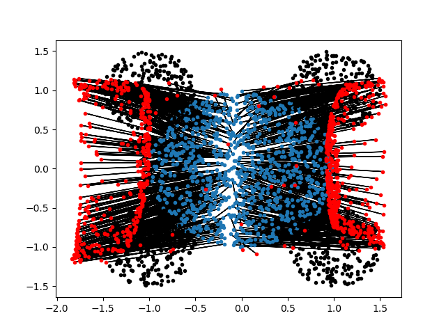
The flow sym_discr benefits a little bit by adding regularization with tp_sym_discr_5 reaching the minimal . After the first 50% of iterations there is not a real improvement, see Figure 4.9. On visual inspection this flow is quite successful in mapping into the support of while keeping the shapes of and comparable, see Figure 4.10.


The flows based on exp give the best results and greatly benefit from adding the regularization. The algorithm exp reaches the minimum after about 30% of the iterations while tp_exp does not improve substantially after 60% of the iterations, see Figure 4.11. Both flows are quick to map into a measure matching the geometry of , see Figures 4.12 and 4.13.


4.4. Comparison of Adversarial Models
Table 4.2 summarizes the results of trying to learn a transport map following the “adversarial” approach of Subsection 3.4. The name of each model refers to training parameters: for example naming a model adv_l10.0_3_clip_0.01 means that the adversarial term (i.e. the one involving integration over ) in ( A d v ) is “boosted” by multiplying by a factor ; moreover the “3” means that for each gradient descent step for the parameters , 2 gradient ascent steps are performed for the parameters ; finally if “clip” is used, one is specifying the parameter to clip the gradients, e.g. in our case to .
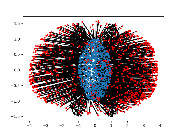
In Figure 4.14 we can inspect the convergence rate of the adversarial models. We see that the “out-of-the-box” parameter seems to yield the best results and gradient clipping does not seems to help. Large values of make the training unstable; for example with there is a steady increase in after about 25% of the training iterations. Inspection of frames shows a lot of chaotic behavior in this case, compare Figure 4.15.
Also increasing the number of iterations of the adversarial network leaves it stuck at a point with a higher value of . The best model is adv_l1_2 which reaches the minimal at around 75% of the iterations. However, the final results are quite disappointing, both in terms of , which is higher than the one obtained simply with the exp flow, and of the final map as lies into a subset of the support of , see Figure 4.16. Generally speaking, we found adversarial training to be under-performing and very sensitive to parameter specification.
In Figure 4.17 we compare the adversarial and the cost component of the loss during the training. We observe that at the beginning of the training (say ) there is a first phase displaying a quick increase in the adversarial component which is then followed by a saturation phase in which the adversarial component stays constant while the cost component increases. The first phase corresponds to the adversarial loss starting to discriminate between and and the second phase to the cost increasing as starts to move towards .
In the training regime (say and ) the adversarial loss continues to grow driving a further rearrangement of inside the support of . Finally, the last phase (say ) is dominated by a degree of reduction of the adversarial loss leading to a collapse of inside the support of . This phenomenon points out that at a certain point the adversarial network starts to fail at discriminating between and . Thus, for the rest of the paper we set the adversarial models aside.
| model name | ||||
|---|---|---|---|---|
| adv_l0.1_2 | 0.70 | 0.010 | 22000 | 50000 |
| adv_l1_10 | 0.49 | 0.013 | 4000 | 50000 |
| adv_l1_2 | 0.37 | 0.037 | 39000 | 50000 |
| adv_l1_2_clip_0.01 | 0.37 | 0.037 | 39000 | 50000 |
| adv_l10_2 | 0.62 | 0.104 | 2000 | 50000 |
| adv_l100_2 | 0.71 | 0.188 | 9000 | 50000 |



4.5. Comparison of Approaches based on duals & supervised learning
In table 4.3 we can see a comparison of the performances of the algorithms based on the dual methods of Subsection 3.5 and supervised learning of Subsection 3.6. The models with a name seguy_.* can use either the entropic or the regularization. Note that the name can contain either “mean” or “sum” depending on how the regularization is aggregated across the batch. In fact, we sum the potentials , on the batch; however, the regularization is a matrix and the mathematical formulation of duality [GCPB16, e.g. Sec. 3] would suggest that we need to sum on one dimension (say ) and take the mean on the other one (say ). However the equations in the original paper [SDF+18, Alg. 1] suggest to use a double sum for the regularization term. While taking the sum degrades a bit the entropic model, it has a positive effect on the -regularized model, which otherwise suffers from a collapsing phenomenon, see Figure 4.18. Overall seguy_ent_mean and seguy_l2_sum have comparable performances, see Figures 4.19 and 4.20, with the latter requiring less iterations.
In Figure 4.21 we can see the convergence rate for the models using a supervised approach. Except for supervised_prob all these models have a higher variance but, except for supervised_prob, the final performance is comparable to the one of seguy_ent_mean and seguy_l2_sum.
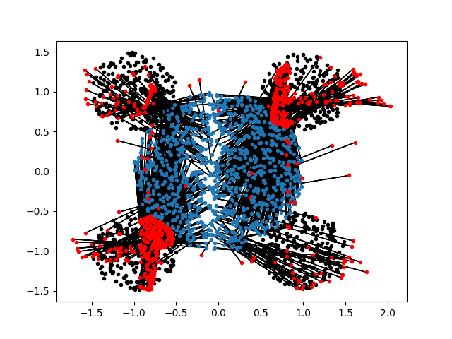
In the model supervised_prob we try to first learn a transport plan and then use the heuristic ( heur → π T ) to learn a transport map. In practice this model performs poorly and the starts to grow; on a qualitative inspection we observe that the first plans tend to distort the geometry of relatively to that of , while towards the end of the training becomes too diffused, see Figure 4.22. Finally, we also point out that the training of this model is considerably slower than for the others as it requires fitting a neural network for the plan against a matrix (while for potentials or maps we fit against vectors of size ).
Both the methods based on the supervised dual or the supervised map perform well. The high variance seems to be an artifact of the iterations using supervised data and can be reduced in practice by using a validation rule which decides when to stop the fitting of the map . Concretely, periodically one evaluates the performance of against a “ground-truth” to decide when to stop the training of . Note that even with the high variance the maps tend to stay qualitatively closed to , i.e. we do not observe phenomena like collapsing or diffusion, see Figure 4.23. Finally, we point out that the approach based on directly learning is faster while both the models seguy_.* and supervised_dual_.* require a second step to fit .
| model name | ||||
|---|---|---|---|---|
| seguy_ent_mean_0.1 | 0.15 | 0.021 | 9200 | 10000 |
| seguy_ent_sum_0.1 | 0.17 | 0.016 | 9200 | 10000 |
| seguy_l2_mean_0.1 | 0.27 | 0.012 | 4500 | 5000 |
| seguy_l2_sum_0.1 | 0.15 | 0.019 | 4500 | 5000 |
| supervised_dual_0.05 | 0.21 | 0.093 | 13800 | 30600 |
| supervised_dual_0.1 | 0.18 | 0.082 | 14000 | 20800 |
| supervised_map_iters_1000_0.05 | 0.16 | 0.096 | 24000 | 51000 |
| supervised_map_iters_200_0.05 | 0.18 | 0.084 | 8000 | 50000 |
| supervised_prob | 0.29 | 0.030 | 3000 | 51000 |


4.6. Timings
We now discuss the time consumption for the models that we find more promising, see Table 4.4. We ran our experiments on a laptop with a -Core Intel (R) Core (TM) i5-5257U@2.70 GHz CPU. We used a docker image of ubuntu:bionic and version 1.0 of PyTorch on Python 3.6.
In Table 4.4 the seconds per step are computed using the wall clock time. The seconds per step are then used to estimate the time to , which we recall was the “best” of the iterations in the snapshots. For models requiring two steps, namely training networks to optimize a dual problem and use the potentials to learn a transport map, we report two rows of timings, one for the dual and another for the map. While secs per step is an objective metric, secs to must be taken with a grain of salt as it depends on the parameters used to run the corresponding script.
In general, total timings are relatively comparable. However, we see the advantage of using models like tp_exp or supervised_map_iters_1000_0.05 that learn directly the transport map. Using Sinkhorn iterations also gives a speed up compared to using the dual problem. For example in seguy_l2_sum_0.1 about seconds are required for each step of the dual problem, compared to the required by supervised_dual_0.1.
| model name | secs per step | secs to |
|---|---|---|
| tp_exp | 0.00456 | 123.04 |
| supervised_map_iters_1000_0.05 | 0.00303 | 72.60 |
| seguy_l2_sum_0.1 (dual) | 0.00795 | 35.78 |
| seguy_l2_sum_0.1 (map) | 0.01192 | 59.60 |
| seguy_ent_mean_0.1 (dual) | 0.00806 | 74.18 |
| seguy_ent_mean_0.1 (map) | 0.01245 | 124.48 |
| supervised_dual_0.1 (dual) | 0.00482 | 67.48 |
| supervised_dual_0.1 (map) | 0.00607 | 60.70 |
4.7. Conclusion
We have compared a variety of approaches to find an optimal map between probability distributions.
We find that, despite different theoretical/heuristic justifications, some algorithms yield similar good optimal maps. Specifically, we find flows using local Gaussian bumps, supervised learning approaches learning potentials or directly a transport map and the dual formulation of [SDF+18] to yield good results. In terms of time consumption, algorithms learning directly the transport map and using Sinkhorn’s iterations are more favorable.
On the other hand, we also find other approaches to under-perform or being unstable. In particular, flows using the covariance loss or the discr @ seem to yield poor maps. Approaches using adversarial training yield poor maps and are also unstable to train.
References
- [AB17] Martin Arjovsky and Léon Bottou. Towards Principled Methods for Training Generative Adversarial Networks. arXiv e-prints, page arXiv:1701.04862, Jan 2017.
- [ACB17] Martin Arjovsky, Soumith Chintala, and Léon Bottou. Wasserstein GAN. arXiv e-prints, page arXiv:1701.07875, Jan 2017.
- [Cut13] Marco Cuturi. Sinkhorn distances: Lightspeed computation of optimal transport. In Proceedings of the 26th International Conference on Neural Information Processing Systems - Volume 2, NIPS’13, pages 2292–2300, USA, 2013. Curran Associates Inc.
- [GCPB16] Aude Genevay, Marco Cuturi, Gabriel Peyré, and Francis Bach. Stochastic optimization for large-scale optimal transport. In Proceedings of the 30th International Conference on Neural Information Processing Systems, NIPS’16, pages 3440–3448, USA, 2016. Curran Associates Inc.
- [GM17] Samuel Gerber and Mauro Maggioni. Multiscale strategies for computing optimal transport. CoRR, abs/1708.02469, 2017.
- [GPAM+14] Ian Goodfellow, Jean Pouget-Abadie, Mehdi Mirza, Bing Xu, David Warde-Farley, Sherjil Ozair, Aaron Courville, and Yoshua Bengio. Generative adversarial nets. In Z. Ghahramani, M. Welling, C. Cortes, N. D. Lawrence, and K. Q. Weinberger, editors, Advances in Neural Information Processing Systems 27, pages 2672–2680. Curran Associates, Inc., 2014.
- [KS12] S. Shunmuga Krishnan and Ramesh K. Sitaraman. Video stream quality impacts viewer behavior: Inferring causality using quasi-experimental designs. In Proceedings of the 2012 Internet Measurement Conference, IMC ’12, pages 211–224, New York, NY, USA, 2012. ACM.
- [KSKW15] Matt Kusner, Yu Sun, Nicholas Kolkin, and Kilian Weinberger. From word embeddings to document distances. In Francis Bach and David Blei, editors, Proceedings of the 32nd International Conference on Machine Learning, volume 37 of Proceedings of Machine Learning Research, pages 957–966, Lille, France, 07–09 Jul 2015. PMLR.
- [LA08] Giuseppe Savare Luigi Ambrosio, Nicola Giglio. Gradient Flows In Metric Spaces and in the Space of Probability Measures. Birkhäuser Basel, 2008. Available at: http://www2.stat.duke.edu/ sayan/ambrosio.pdf.
- [LV09] John Lott and Cédric Villani. Ricci curvature for metric-measure spaces via optimal transport. Annals of Mathematics, 169(3):903–991, 2009.
- [Net] Netflix. Quasi experimentation at netflix. https://medium.com/netflix-techblog/quasi-experimentation-at-netflix-566b57d2e362. Technology Blog (Sep 2018), Accessed at: 2019-07-30.
- [OZM+16] Darya Y. Orlova, Noah Zimmerman, Stephen Meehan, Connor Meehan, Jeffrey Waters, Eliver E. B. Ghosn, Alexander Filatenkov, Gleb A. Kolyagin, Yael Gernez, Shanel Tsuda, Wayne Moore, Richard B. Moss, Leonore A. Herzenberg, and Guenther Walther. Earth mover’s distance (emd): A true metric for comparing biomarker expression levels in cell populations. PLOS ONE, 11(3):1–14, 03 2016.
- [PC19] Gabriel Peyré and Marco Cuturi. Computational optimal transport. Foundations and Trends® in Machine Learning, 11(5-6):355–607, 2019.
- [PvF+18] Giorgio Patrini, Rianne van den Berg, Patrick Forré, Marcello Carioni, Samarth Bhargav, Max Welling, Tim Genewein, and Frank Nielsen. Sinkhorn AutoEncoders. arXiv e-prints, page arXiv:1810.01118, Oct 2018.
- [San15] Filippo Santambrogio. Optimal Transport for Applied Mathematicians. Birkhäuser Basel, 2015. Available at: https://www.math.u-psud.fr/filippo/OTAM-cvgmt.pdf.
- [SDF+18] Vivien Seguy, Bharath Bhushan Damodaran, Rémi Flamary, Nicolas Courty, Antoine Rolet, and Mathieu Blondel. Large-scale optimal transport and mapping estimation. In Proceedings of the International Conference in Learning Representations, 2018.
- [SdGP+15] Justin Solomon, Fernando de Goes, Gabriel Peyré, Marco Cuturi, Adrian Butscher, Andy Nguyen, Tao Du, and Leonidas Guibas. Convolutional wasserstein distances: Efficient optimal transportation on geometric domains. ACM Trans. Graph., 34(4):66:1–66:11, July 2015.
- [SK67] Richard Sinkhorn and Paul Knopp. Concerning nonnegative matrices and doubly stochastic matrices. Pacific J. Math., 21(2):343–348, 1967.
- [TT16] Giulio Trigila and Esteban G. Tabak. Data-driven optimal transport. Communications on Pure and Applied Mathematics, 69(4):613–648, 2016.
- [WB17] Jonathan Weed and Francis Bach. Sharp asymptotic and finite-sample rates of convergence of empirical measures in Wasserstein distance. arXiv e-prints, page arXiv:1707.00087, Jun 2017.
- [ZML16] Junbo Zhao, Michael Mathieu, and Yann LeCun. Energy-based Generative Adversarial Network. arXiv e-prints, page arXiv:1609.03126, Sep 2016.