Surpassing the rate-transmittance linear bound of quantum key distribution

Xiao-Tian Fang

{}^{1,\,2,\,*}

Affiliation: ¹Hefei National Laboratory for Physical Sciences at Microscale and Department of Modern Physics, University of Science and Technology of China, Hefei, Anhui 230026, China Pei Zeng

{}^{3,\,*}

Affiliation: ¹Hefei National Laboratory for Physical Sciences at Microscale and Department of Modern Physics, University of Science and Technology of China, Hefei, Anhui 230026, China Hui Liu

{}^{1,\,2,\,*}

Affiliation: ¹Hefei National Laboratory for Physical Sciences at Microscale and Department of Modern Physics, University of Science and Technology of China, Hefei, Anhui 230026, China Mi Zou^1, 2 Affiliation: ¹Hefei National Laboratory for Physical Sciences at Microscale and Department of Modern Physics, University of Science and Technology of China, Hefei, Anhui 230026, China Weijie Wu³ Affiliation: ¹Hefei National Laboratory for Physical Sciences at Microscale and Department of Modern Physics, University of Science and Technology of China, Hefei, Anhui 230026, China Yan-Lin Tang⁴ Affiliation: ¹Hefei National Laboratory for Physical Sciences at Microscale and Department of Modern Physics, University of Science and Technology of China, Hefei, Anhui 230026, China Ying-Jie Sheng⁴ Affiliation: ¹Hefei National Laboratory for Physical Sciences at Microscale and Department of Modern Physics, University of Science and Technology of China, Hefei, Anhui 230026, China Yao Xiang⁴ Affiliation: ¹Hefei National Laboratory for Physical Sciences at Microscale and Department of Modern Physics, University of Science and Technology of China, Hefei, Anhui 230026, China Weijun Zhang⁵ Affiliation: ¹Hefei National Laboratory for Physical Sciences at Microscale and Department of Modern Physics, University of Science and Technology of China, Hefei, Anhui 230026, China Hao Li⁵ Affiliation: ¹Hefei National Laboratory for Physical Sciences at Microscale and Department of Modern Physics, University of Science and Technology of China, Hefei, Anhui 230026, China Zhen Wang⁵ Affiliation: ¹Hefei National Laboratory for Physical Sciences at Microscale and Department of Modern Physics, University of Science and Technology of China, Hefei, Anhui 230026, China Lixing You⁵ Affiliation: ¹Hefei National Laboratory for Physical Sciences at Microscale and Department of Modern Physics, University of Science and Technology of China, Hefei, Anhui 230026, China Ming-Jun Li⁶ Affiliation: ¹Hefei National Laboratory for Physical Sciences at Microscale and Department of Modern Physics, University of Science and Technology of China, Hefei, Anhui 230026, China Hao Chen⁶ Affiliation: ¹Hefei National Laboratory for Physical Sciences at Microscale and Department of Modern Physics, University of Science and Technology of China, Hefei, Anhui 230026, China Yu-Ao Chen^1, 2 Affiliation: ¹Hefei National Laboratory for Physical Sciences at Microscale and Department of Modern Physics, University of Science and Technology of China, Hefei, Anhui 230026, China Qiang Zhang^1, 2 Affiliation: ¹Hefei National Laboratory for Physical Sciences at Microscale and Department of Modern Physics, University of Science and Technology of China, Hefei, Anhui 230026, China Cheng-Zhi Peng^1, 2, 4 Affiliation: ¹Hefei National Laboratory for Physical Sciences at Microscale and Department of Modern Physics, University of Science and Technology of China, Hefei, Anhui 230026, China Xiongfeng Ma³ Affiliation: ¹Hefei National Laboratory for Physical Sciences at Microscale and Department of Modern Physics, University of Science and Technology of China, Hefei, Anhui 230026, China Teng-Yun Chen^1, 2 Affiliation: ¹Hefei National Laboratory for Physical Sciences at Microscale and Department of Modern Physics, University of Science and Technology of China, Hefei, Anhui 230026, China Jian-Wei Pan^1, 2 Affiliation: ¹Hefei National Laboratory for Physical Sciences at Microscale and Department of Modern Physics, University of Science and Technology of China, Hefei, Anhui 230026, China Affiliation: ²CAS Center for Excellence in Quantum Information and Quantum Physics, University of Science and Technology of China, Hefei, Anhui 230026, China Affiliation: ³Center for Quantum Information, Institute for Interdisciplinary Information Sciences, Tsinghua University, Beijing 100084, China Affiliation: ⁴QuantumCTek Corporation Limited, Hefei, Anhui 230088, China Affiliation: ⁵State Key Laboratory of Functional Materials for Informatics, Shanghai Institute of Microsystem and Information Technology, Chinese Academy of Sciences, Shanghai 200050, China Affiliation: ⁶Corning Incorporated, Corning, New York 14831, USA Affiliation: ^∗These authors contributed equally to this work.

August 11, 2026

Abstract

Quantum key distribution (QKD)Bennett and Brassard 1984; Ekert 1991 offers a long-term solution to establish information-theoretically secure keys between two distant users. In practice, with a careful characterization of quantum sources and the decoy-state methodHwang 2003; Lo et al. 2005; Wang 2005, measure-device-independent quantum key distribution (MDI-QKD)Lo et al. 2012 provides secure key distribution. While short-distance fibre-based QKD has already been available for real-life implementationTang et al. 2014, the bottleneck of practical QKD lies on the limited transmission distance. Due to photon losses in transmission, it was believed that the key generation rate is bounded by a linear function of the channel transmittance, $O(\eta)$ , without a quantum repeaterTakeoka et al. 2014; Pirandola et al. 2017, which puts an upper bound on the maximal secure transmission distanceYin et al. 2016; Boaron et al. 2018. Interestingly, a new phase-encoding MDI-QKD scheme, named twin-field QKDLucamarini et al. 2018, has been suggested to beat the linear bound, while another variant, named phase-matching quantum key distribution (PM-QKD), has been proven to have a quadratic key-rate improvementMa et al. 2018; Lin and Lütkenhaus 2018, $O(\sqrt{\eta})$ . In reality, however, the intrinsic optical mode mismatch of independent lasers, accompanied by phase fluctuation and drift, impedes the successful experimental implementation of the new schemes. Here, we solve this problem with the assistance of the laser injection technique and the phase post-compensation method. In the experiment, the key rate surpasses the linear key-rate bound via 302 km and 402 km commercial-fibre channels, achieving a key rate over 4 orders of magnitude higher than the existing results in literatureYin et al. 2016. Furthermore, with a 502 km ultralow-loss fibre, our system yields a secret key rate of 0.118 bps. We expect this new type of QKD schemes to become a new standard for future QKD.

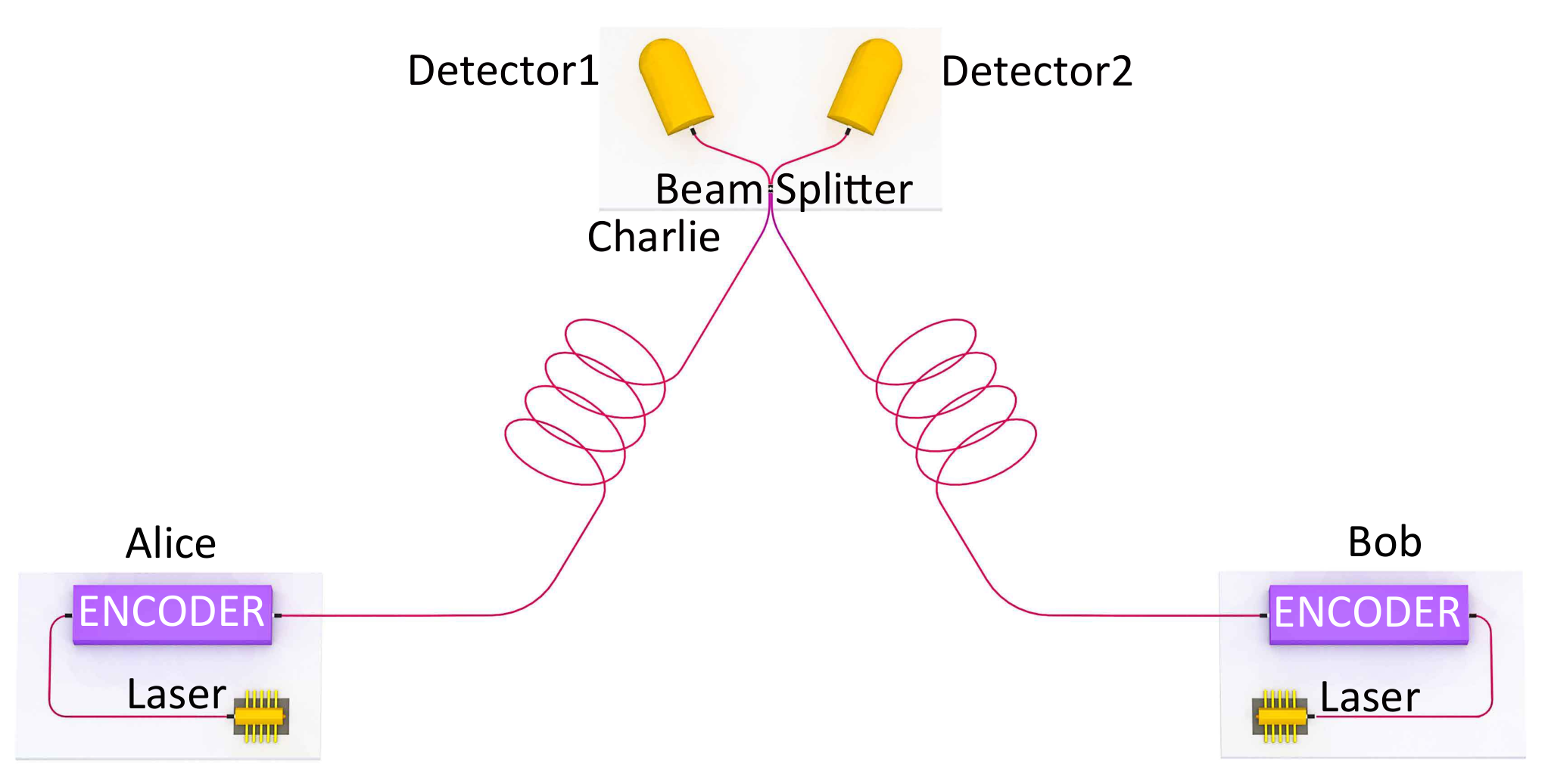
In conventional point-to-point QKD, such as the BB84 protocolBennett and Brassard 1984, the sender Alice encodes key information into quantum states and sends them to the receiver Bob for detection. Whereas in MDI-QKD, Alice’s and Bob’s positions are symmetric. They both send out encoded optical pulses to a measurement site owned by Charlie, who interferes the pulses and publicly announces the results to correlate Alice’s and Bob’s key information. The security of MDI-QKD does not depend on how Charlie realizes the measurement or announces the results. As a result, this scheme is immune to all attacks on the detection and hence owns a higher security level in practice.

In quantum communication, attenuated lasers are widely used as photon sources, which can be described by weak coherent states, $\ket{\alpha}=e^{-|\alpha|^{2}/2}\sum_{k=0}^{\infty}\frac{\alpha^{k}}{k!}\ket{k}$ , superpositions of $k$ -photon states $\ket{k}$ . The parameter $\alpha=\sqrt{\mu}e^{i\phi}$ is a complex number, where $\mu=|\alpha|^{2}$ is the light intensity and $\phi$ is the phase. In the original MDI-QKDLo et al. 2012, the user encodes the key information into two weak coherent states on two orthogonal optical modes, such as polarization encoding. In the security analysis, only the information carried by the single-photon states can be used for the final key generation. The decoy-state method is widely employed to efficiently extract secret key informationHwang 2003; Lo et al. 2005; Wang 2005.

In reality, quantum information carriers, photons, can be easily lost during transmission. Define the transmittance between Alice and Bob $\eta$ to be the probability of a photon being successfully transmitted through the channel and being detected. Hence, in the symmetric setting of MDI-QKD, the transmittance between Alice (Bob) and the measurement site is $\sqrt{\eta}$ . Only the detections, caused by Alice’s and Bob’s single-photon states, can be used for secure key generation. Then such detection rate is given by $O(\eta)$ , as a natural upper bound of the key rate.

To achieve a better rate-transmittance performance, a new phase-encoding MDI-QKD scheme, named PM-QKD, has been proposed, as shown in Fig. 1. Alice (Bob) encodes the key information into the phase of a coherent state on a single optical mode. In this case, Charlie treats Alice and Bob’s two optical modes as one quantum system and detects the relative phase between them. To do so, Charlie only needs one photon in the joint quantum system. Therefore, the detection rate is $O(\sqrt{\eta})$ . Strict security analysis shows that PM-QKD enjoys a quadratic improvement on the rate-transmittance performance over the original MDI-QKDMa et al. 2018.

Refer to caption — Figure 1: Schematic diagram of PM-QKD. Encoder is a device to modulate the intensity $\mu$ and phase $\phi$ of coherent states. The beam splitter and the single photon detectors are used for interference detection. Divide the phases $\phi\in[0,2\pi)$ into $D$ slices, denoted by $\Delta_{j}=\left[\frac{\pi}{D}(2j-1),\frac{\pi}{D}(2j+1)\right)$ with the index $0\leq j\leq D-1$ . In the experiment, we set $D=16$ . In each round of key distribution, Alice encodes a random bit $\kappa_{a}$ into her coherent state $\ket{\sqrt{\mu_{a}}e^{i(\kappa_{a}\pi+\phi_{a})}}$ , after adding an extra discrete random phase $\phi_{a}=j_{a}2\pi/D$ which is at the center of $j_{a}$ th phase slice $\Delta_{j_{a}}$ . Similarly, Bob encodes $\kappa_{b}$ , $\mu_{b}$ , and $\phi_{b}$ on his pulse, $\ket{\sqrt{\mu_{b}}e^{i(\kappa_{b}\pi+\phi_{b})}}$ . Alice and Bob then send their pulses to Charlie, who is supposed to interfere these quantum states to measure phase differences. After Charlie announces the detection results, Alice and Bob publicly announce the slice indexes $j_{a},j_{b}$ of the random phases. They post-select the key bits $\kappa_{a},\kappa_{b}$ as the raw key, according to Charlie’s detection results and the sifting scheme depending on $j_{a},j_{b}$ , with the phase post-compensation technique.

Despite the promising qualities of PM-QKD on both security and performance, the experimental implementation is very challenging. In PM-QKD, the interference results at the measurement result should reflect the difference between Alice’s and Bob’s encoded phases. In practice, an essential requirement is to match the phases of coherent states generated by two remote and independent lasers. The coherent states of Alice $\ket{\sqrt{\mu_{a}}e^{i(\kappa_{a}\pi+\phi_{a})}}$ and Bob $\ket{\sqrt{\mu_{b}}e^{i(\kappa_{b}\pi+\phi_{b})}}$ could have different phase references due to phase drift and fluctuation. Define the reference deviation $\phi_{\delta}$ to be the phase difference when both Alice and Bob set $\kappa_{a(b)}=0$ and $\phi_{a(b)}=0$ . There are three main factors determining the value of $\phi_{\delta}$ , fluctuations of the laser initial phases, fibre lengths, and laser frequencies. Take the $1550$ nm telecom light through a $200$ km fibre for example, either a tiny change of transmission time, say by $10^{-15}$ s corresponding to a 200 nm optical length, or a small deviation of the angular frequency, say by 1 kHz, will cause a significant phase drift. Note that, there are several recent experiments which make efforts to deal with these challenges in order to demonstrate the advantages of the new type of MDI-QKD schemesMinder et al. 2019; Liu et al. 2019; Wang et al. 2019; Zhong et al. 2019.

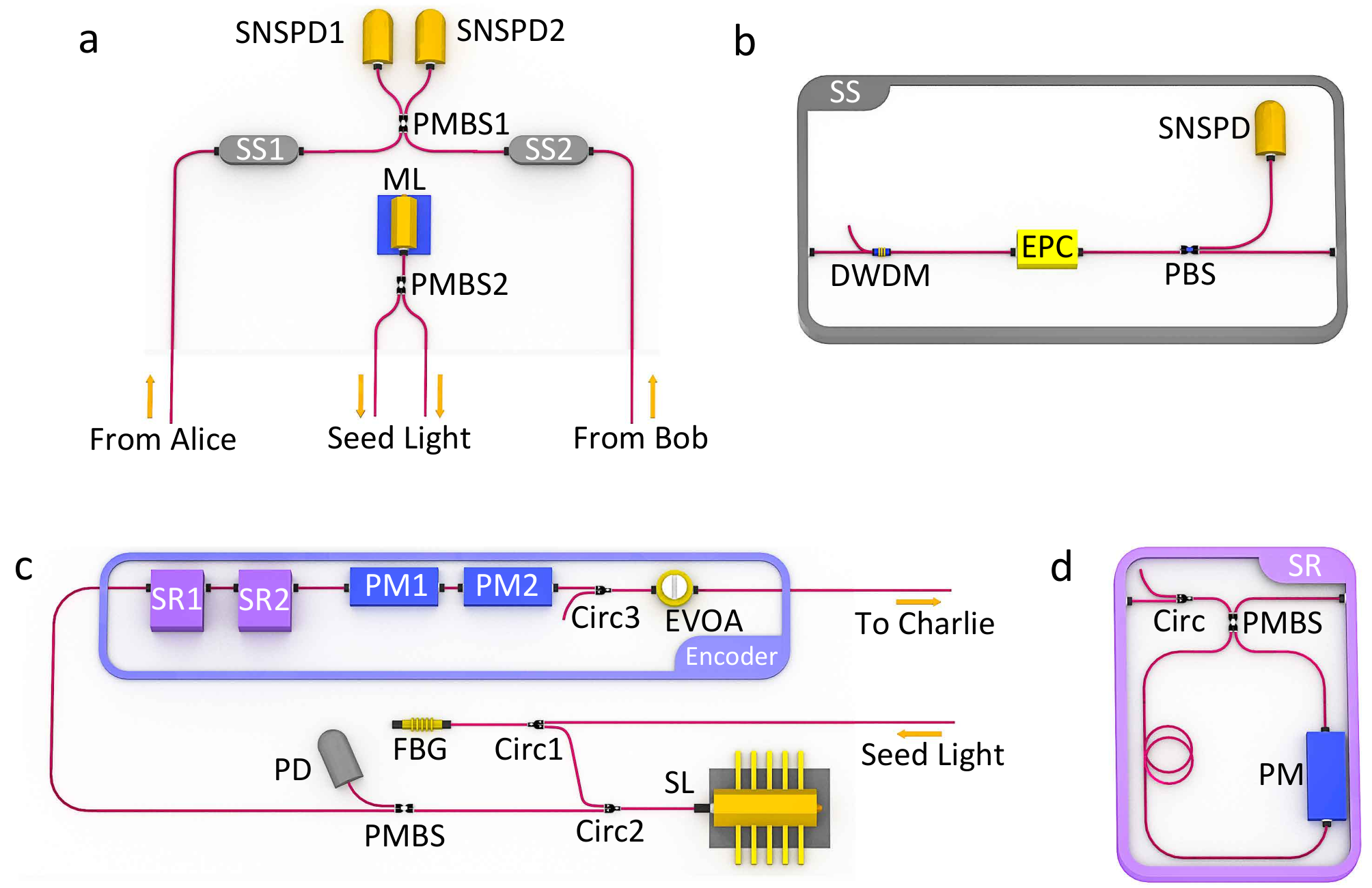
In this work, we implement PM-QKD with the setup shown in Fig. 2. In order to suppress the fluctuations of the laser initial phases and frequencies, we employ the laser injection techniqueLipka et al. 2017. The setups on Alice’s and Bob’s sides are exactly the same. Below, we take Alice’s side for example. The master laser in between Alice and Bob, with 3 kHz line-width and 1550.12 nm centre wavelength, emits a seed light which goes through a long fibre to lock Alice’s distributed feedback laser. Alice’s laser generates optical pulses with a clock rate of 312.5 MHz. Two Sagnac rings are employed to modulate pulses into four different intensities. The pulses with the largest intensity are used as reference pulses for phase estimation, while the other three pulses are used as the signal state, weak decoy state, and vacuum state to implement the decoy-state method. The extinction ratio between the signal state and the vacuum state is about 20 dB. Two phase modulators are employed to modulate 16 different phases. Details of the laser injection technique and the phase estimation are presented in Appendix A and B.

The pulses from Alice and Bob are transmitted through long optical fibres and interfered at the measurement site. The interference results are detected by two superconducting nanowire single photon detectors. The dark count is about $10$ counts per second and the detector efficiency is about $40\%$ . The total detection efficiency reduces to about $23\%$ owing to 1.2 dB insertion loss and $25\%$ non-overlapping between signal and detection windows. Two stabilization systems are inserted before interference to filter out the noise caused by the nonlinear effect of the fibre and stabilizing the incident pulses. Details of the implementation are presented in Appendix D.

Due to fibre fluctuation, there exists a slow phase drift between Alice and Bob. In the case when the phase fluctuates slowly, pulses nearby share similar values of the reference deviation $\phi_{\delta}$ . Inspired by this observation, we employ a simple phase post-compensation techniqueMa and Razavi 2012. During the experiment, Alice and Bob send reference pulses and quantum pulses periodically. The reference pulse is typically more than one order of magnitude stronger than the quantum pulse. They use reference pulses to estimate which slice $j_{\delta}$ the reference deviation $\phi_{\delta}$ lies in, according to interference results. They use quantum pulses to perform the PM-QKD experiment. After obtaining measurement results, Alice and Bob publicly announce the random phase slices $j_{a},j_{b}$ of the signal pulses. They calculate $j_{s}=j_{a}-j_{b}+j_{\delta}$ for raw key sifting, where $j_{\delta}$ works as the post-compensation shift. Clearly, if $j_{\delta}$ accurately reflects the real-time reference deviation of the system, perfect interference will happen when $j_{s}=0$ or $j_{s}=8$ . Note that the estimated phase slice indexes $j_{\delta}$ are only used in the post-processing, which frees us from active phase locking during the state transmission. Furthermore, compared with active locking, where the phase can only be locked well when $\phi_{\delta}$ keeps stable during the whole process of phase estimation and feedback, the phase post-compensation method can tolerate faster fluctuation, as long as $\phi_{\delta}$ does not change much in the time between the reference and quantum pulses.

In the security analysis of PM-QKDMa et al. 2018, due to the random phases Alice and Bob modulated on their coherent states, the joint state can be decomposed into odd and even total photon number components, $\rho^{odd}_{AB}$ and $\rho^{even}_{AB}$ . Denote the proportions of detection caused by $\rho^{odd}_{AB}$ and $\rho^{even}_{AB}$ as $q^{odd}$ and $q^{even}$ , respectively, and obviously, $q^{odd}+q^{even}=1$ . In fact, the information leakage in PM-QKD is shown to be independent of channel disturbance. As a result, the privacy is only related to $q^{even}$ , irrelevant to the bit error rate. The final key length is given by

K=M_{\mu}[1-H(q^{even}_{\mu})]-l_{cor},

(1)

where $H(x)=-x\log_{2}x-(1-x)\log_{2}(1-x)$ is the binary entropy function. Here, we consider the case where Alice and Bob use the same intensities of coherent states. The subscript $\mu$ represents the signal states with $\mu_{a}=\mu_{b}=\mu/2$ . The raw key length $M_{\mu}$ is the number of detection events caused by signal states when Alice and Bob match their phases, $j_{s}=0$ or $8$ . The even photon component ratio $q^{even}_{\mu}$ can be efficiently estimated by decoy state methodsHwang 2003; Lo et al. 2005; Wang 2005. The error correction cost $l_{cor}$ can be usually estimated by a function of bit error rate $E_{\mu}$ , $l_{cor}=fM_{\mu}H(E_{\mu})$ , where $f$ is the error correction efficiency depending on $E^{j_{s}}_{\mu}$ . The key rate is defined by $R=K/N$ , where $N$ is the number of QKD rounds. Details of the decoy state method and the security analysis by considering the finite data size effects are presented in Appendix E.

In order to further improve the key rate, one can take advantage of the data with mismatched phases. Note that the phase-mismatched signals of $j_{s}=1,9$ can be regarded as the ones with a fixed misalignment $\phi_{\delta}=2\pi/D$ , which results in a larger bit error rate compared with the phase-matched signals of $j_{s}=0,8$ . The raw keys with different $j_{s}$ have the same $q^{even}$ in Eq. (1) and hence the same privacy. More explicitly, Alice and Bob can categorize the data from signal states into $D/2$ groups, where the data of $j_{s}=0,8$ are in the $0$ -th group, the data of $j_{s}=1,9$ are in the $1$ -st group, etc. Alice and Bob can correct errors in each data group separately and perform privacy amplification altogether. Of course, if the error rate in a group is too large, they can simply discard that group of data.

We perform the experiment via $101$ , $201$ , $302$ , $402$ km standard optical fibres and a $502$ km ultralow-loss optical fibre. The experiment parameters and results are presented in Fig. 3, from which one can see that the key rate-transmittance relation follows $R=O(\sqrt{\eta})$ as a contrast with the linear rate-transmittance bound. Specifically, the experimental results beat the linear bound at the distances of $302$ and $402$ km. Take the 302 km fibre case as an example, with the same channel transmission and detection efficiency, the linear key-rate bound is given by $R_{up}=5.44\times 10^{-7}$ . Our experiment yields a key rate of $R=6.74\times 10^{-7}$ , with a failure probability of $\epsilon=1.68\times 10^{-10}$ , when all the mismatched data is used. The key rate is $24.0\%$ higher than the bound. In the case of 302 km, the data with mismatched phases has a significant contribution to the overall key rate, which is $72.6\%$ larger than the value with only the phase-matched group considered. Notably, our achieved key rate is three orders of magnitude higher than the asymptotic key rate of the original MDI-QKD schemeLo et al. 2012.

Meanwhile, we obtain a positive key rate at $502$ km experiment with an ultralow-loss optical fibre, beating the current record of 421 km fibre communication distance of QKDBoaron et al. 2018. The channel loss of $502$ km experiment is 81.7 dB and the total loss is 87.1 dB. This new loss-tolerance record is comparable with the high-orbital satellite link loss in free space.

Figure 3: Experimental parameters and results. a. Main panel, the experimental rate-distance performance of PM-QKD, comparing with the theoretical expectation and the linear key rate bound Pirandola et al. 2017. The data points marked by cross and star are, respectively, the key rate without and with the usage of phase-mismatched signals. Inset, error rate against total loss. The solid line shows the bit error rate in the theoretical model, and the crosses show the experiment data. b. The bit error rate with respect to the experiment time in the

302

km experiment. Each data point represents a number of

3.31\times 10^{5}

effective clicks which are collected in

21.91

minutes on average. The blue dots and red dots show the bit error rate for data with phase difference

j_{d}=0

and

1

, respectively. c. Parameters used in the experiment and theoretical simulation. Note that, the listed value of the dark count rate

p_{d}

, the detection efficiency

\eta_{d}

, misalignment error

e_{d}

, and the fibre loss of PM-QKD are used for numerical simulation. The corresponding experimental values depend on the specific environment, which are listed in Appendix G.

Our results show that PM-QKD system is stable and economical, which facilitates the promotion of practical QKD. In the future, we expect to use the phase post-compensation technique to keep the system robust by increasing the system repetition frequency and enhancing the detectors’ performance. Also, we expect that the design of PM-QKD experiment will be helpful for the construction of quantum repeaterZukowski et al. 1993; Briegel et al. 1998, as well as extending the reach of the quantum internet.

Funding Information

This work has been supported by the National Key R&D Program of China (Grant No. 2017YFA0303903 and No. 2017YFA0304000), the Chinese Academy of Science, the National Fundamental Research Program, the National Natural Science Foundation of China (Grant No. 11875173, No. 61875182 and No. 11674193), Anhui Initiative in Quantum Information Technologies, and Fundamental Research Funds for the Central Universities (WK2340000083).

Acknowledgments

We acknowledge H. Zhou for the insightful discussions.

Author Contributions

All authors contributed extensively to the work presented in this paper.

Author Information

Reprints and permissions information is available at www.nature.com/reprints. The authors declare no competing financial interests. Readers are welcome to comment on the online version of this article at www.nature.com/nature.

Appendix A Phase drift estimation

Rather than using extra devices to lock the phase, here we apply the phase estimation method to estimate the drifted phase, as shown in Fig. 4. Here, Alice and Bob need not obtain the exact value of the real-time phase deviation $\phi_{\delta}$ , but only an estimation of the slice number $j_{\delta}$ for post-compensation. Moreover, the estimation of $j_{\delta}$ does not need to be announced in a real-time manner. Instead, it can be announced during the sifting process, as a post-selection shift factor. This makes our protocol practical without active feedback.

In the reference pulse region, Alice and Bob send reference pulses to Charlie, who interferes them and announces the results. They use the interference results to estimate the phase slice difference between two reference pulses, $\phi_{\delta}$ . The right detector click ratio $P_{r}$ after interference is

\frac{n_{r}}{n_{r}+n_{l}}\approx P_{r}=\frac{1+\cos\phi_{\delta}}{2},

(2)

where $n_{r}$ and $n_{l}$ are the counts of the right and left detector clicks, respectively. With this ratio, one can classify the phase fluctuation $\phi_{\delta}$ to the phase slices $\Delta_{j_{\delta}}$ marked by $j_{\delta}$ according to the detection ratio.

Note that, since the phase deviation $\phi_{\delta}$ and $(2\pi-\phi_{\delta})$ yield the same $P_{r}$ , Alice and Bob cannot discriminate these two cases from the ratio $P_{r}$ . To solve this problem, Alice loads a $\phi_{0}=\pi/2$ phase on the pulses in the latter reference pulse region, making the phase difference to be $\phi_{\delta}+\pi/2$ , and hence $P_{r}=\frac{1-\sin\phi_{\delta}}{2}$ . In that case, one can distinguish the phase slice $j_{\delta}$ from $(16-j_{\delta})$ . With the interference results $P_{r}$ from the case $\phi_{0}=0$ and $\phi_{0}=\pi/2$ , Alice and Bob can estimate $j_{\delta}$ accurately, as shown in Fig. 5.

Figure 5: Phase estimation region. The blue, green, red and orange region denotes four phase quadrants ranging from

[0,\pi/2)

[\pi/2,\pi)

[\pi,3\pi/2)

, and

[3\pi/2,2\pi)

. The solid line shows the theoretic detection probability

P_{r}

with the initial phase difference

\phi_{0}

of the reference pulse is set to

0

, while the dashed line shows

P_{r}

when

\phi_{0}=\pi/2

. From these two estimated

P_{r}

values, one can infer the

j_{\delta}

value with no degeneracy.

In order to yield an accurate estimation of $j_{\delta}$ , sufficient detection counts of the reference pulses are required. According to the transmittance and phase drift velocity, one should properly set the intensity and time duration of the reference pulse and the system repetition frequency.

Appendix B Laser injection technique

The fluctuation of reference deviation $\phi_{\delta}$ is mainly caused by three factors: the initial phase fluctuation of the lasers, the optical length fluctuation, and the fluctuation of the laser frequencies. In order to minimize the fluctuation caused by the first and the third factors, we apply the laser injection technique.

As shown in Fig. 6a, a narrow line-width continuous wave laser at Charlie side works as the master laser, while DFB laser at Alice’s (same as Bob’s) side works as the slave laser. The seed light generated by the master laser is divided into two parts and sent to the two slave lasers through long fibres, which induces stimulated emission. In this case, the wavelength and phase of the light generated by the slave laser are the same as the seed light, which results in slower fluctuation of laser initial phases. For a local experiment test, interference results of pulses generated by slave lasers shows that the phase difference of two locked slave lasers fluctuates in a relatively low speed, which is presented in Fig. 6b. Here, the residual phase noise and fluctuation mainly come from the spontaneous emission in the slave lasers. Though the phase will fluctuate faster when the fibre gets longer, we can still get an effecive phase estimation in this case.

In the $101$ , $201$ , $302$ km experiments, the master laser is put at the middle point between Alice and Bob’s laser. The fibres used to transmit seed light and the signal light are different but with the same length. Due to the limited power of the master laser and low transmittance value, in the $402$ km and $502$ km experiments, we place the master laser and the slave lasers locally.

Appendix C PM-QKD protocol

In Box. C, we explicitly present the phase-matching quantum key distribution (PM-QKD) scheme implemented in the experiment. We divide the phase space $0\sim 2\pi$ into $D$ slices and denote the $j$ -th slice as $\Delta_{j}=[\frac{\pi}{D}(2j-1),\frac{\pi}{D}(2j+1))$ . The central phase of $j$ -th slice is $\phi_{j}=\frac{2\pi}{D}j$ .

Suppose the phase references of Alice and Bob are different $\phi^{(0)}_{a},\phi^{(0)}_{b}$ . Moreover, we denote the phase variation in the fibre as $\phi_{f}$ . Before Eve’s interference, the phase difference between Alice and Bob’s pulses is

(\phi_{a}+\phi_{a}^{(0)})-(\phi_{b}+\phi_{b}^{(0)})+\phi_{f}=\phi_{a}-\phi_{b}+(\phi_{a}^{(0)}-\phi_{b}^{(0)}+\phi_{f})=\phi_{a}-\phi_{b}+\phi_{\delta}\approx(j_{a}-j_{b}+j_{\delta})\frac{2\pi}{D},

(3)

and hence the phase difference belongs to the $(j_{a}-j_{b}+j_{\delta})$ -th slice. Suppose $\phi_{\delta}$ fluctuates slowly with respect to time. By the interference of coherent pulses, Alice and Bob can estimate $\phi_{\delta}$ accurately. In this case, for the data with $j_{s}=0$ , the interference should be nearly perfect, with small quantum bit error rate. Note that, the sifting strategy does not affect the security of PM-QKD. It only affects the error correction efficiency.

Appendix D Experiment detail of PM-QKD

D.1 Laser injection details

As is shown in Fig. 7, the continuous wave emitted from the master laser (Realphoton Technology Ltd.) are split by a PMBS and transmitted through long fibres and finally injected into Alice and Bob’s slave laser (Agilecom Ltd.). To achieve a good laser injection result, we apply the Erbium doped fiber amplifier (EDFA) to amplify the light intensity and the dense wavelength division multiplexer (DWDM) to filter the side band noise. After that, a fiber Bragg grating (FBG) inserted before injection is used to block the light with unexpected wavelength. A photoelectric diode (PD) is used to monitor the intensity of injection wave for avoiding that Charlie (or Eve) controls the output of the slave laser by manipulate the injection wave. The optical pulses at the width of 400 ps generated by the slave laser.

Figure 7: Detailed setting of PM-QKD with the nonlocal laser locking system.

D.2 Encoding and measurement devices

In accordance with random bit values generated beforehand, two Sagnac rings Bergh 1993 (SR1-2) are employed to modulate the intensities of reference state and three decoy states while two phase modulators (PM1-2) are employed to modulate encoding phases and random phases. The circulator followed are utilized to prevent Trojan horse attack. Note that the pulse into the SR is split into two pulses by the polarization-maintaining beam splitter (PMBS), one of which travels clockwise and the other travels anticlockwise. The PM in the SR adjusts and loads the phase only on one of the two pulses every round so that the output pulse’s intensity could be modulated when they meet again on the PMBS. To avoid the disturbance on the encoding process, the backward output pulses will be removed by the Circ (circulator) in the SR. Because of the same fiber in which two pulses travel, the clockwise and counter-clockwise paths are insensitive to any length drifts or stress and temperature variation of the fiber within propagation time. In that case, the SR is so stable that the intensity feedback device is unnecessary.

In Charlie’s measurement device, to make sure that the polarization of two pulses are indistinguishable, we utilize two PBSs before interfere to filter unexpected part. The reflection port of each PBS is monitored by the SNSPD with detection efficiency of $20\%$ and dark count rate of 100 cps. Charlie adjusts the DC loaded in the EPC in real time to minimize and stabilize the detection count of SNSPD so the incident pulses intensity for interfere maintains maximum. Note that since we have to send strong reference pulses which is described in Appendix A, we always have enough pulses intensity for the polarization feedback system even the fiber length is up to 500 km, and Our feedback system works well with less than $1\%$ loss of the incident pulse intensity.

The detector efficiency of SNSPD1 and SNSPD2 is about $40\%$ in 101, 201, 302 and 402 km experiments, while in 502 km experiment, we enhance the efficiency of two detectors to $46\%$ and $75\%$ for better performance. To get a higher interference visibility, we set a $25\%$ non-overlap between the signal and detection window. The insertion loss of Charlie’s measurement device is about 1.2 dB.

D.3 Synchronization systems

The entire system are synchronized by two arbitrary-function generators (Tektronix, AFG3253) which is not shown in Fig. 1. Three 100 KHz electric signals in phase are modulated by two arbitrary-function generators. The delay between any two of them is adjustable. Alice, Bob and Charlie use one of them to regenerate their own 312.5 MHz system clock, respectively. To overlap the independent signal pulses from Alice and Bob precisely, we need to develop the time calibration system. First, Charlie measures the arriving time of the optical pulses from Alice and Bob with a time-to-digital converter (TDC), respectively. Then she adjusts the time delay between the electric signals from the arbitrary-function generator according to the calculation of the averaged arriving time. Due to the long optical fiber length drifting, we have to proceed a time calibration every 30 minutes. The total timing calibration precision is about 20 ps which is precise enough for the implement.

Appendix E Finite-size parameter estimation

Here we list the formulas to estimate the key length $K$ , the phase error number, and the corresponding failure probability. The detailed finite-size security analysis of PM-QKD is in Ref. Zeng et al..

E.1 Key length formula

In the experimental PM-QKD protocol introduced in Appendix C, Alice and Bob group the signals by the phase difference $j_{s}$ . For the signals in group $j_{s}$ , the key length is

K^{(j_{s})}=M^{(j_{s})}_{\mu}[1-H(q_{\mu}^{even(j_{s})})]-l_{cor}^{(j_{s})},

(4)

where $M^{\mu(j_{s})}$ is the clicked rounds when Alice and Bob both send out signal lights with $\mu_{i_{a}}=\mu_{i_{b}}=\mu/2$ in the group $j_{s}$ . $q_{\mu}^{even(j_{s})}$ is the estimated fraction caused by the even state

q_{\mu}^{even(j_{s})}=\frac{M^{even(j_{s})}_{\mu}}{M^{(j_{s})}_{\mu}},

(5)

where $M^{even(j_{s})}_{\mu}$ is clicked rounds caused by even photon component in the $M^{(j_{s})}_{\mu}$ with estimation method introduced in Appendix E.2.

The error correction cost, given by $l_{cor}^{(j_{s})}$ , can usually by estimated by a function of bit error rate $E^{(j_{s})}_{\mu}$ among the signals of group $j_{s}$ ,

l_{cor}^{(j_{s})}=fM^{(j_{s})}_{\mu}H(E^{(j_{s})}_{\mu}),

(6)

where $f$ is the error correction efficiency, determined by the error rate $E^{(j_{s})}_{\mu}$ and the specific error correction method. If $E^{(j_{s})}_{\mu}$ is too large, the cost $l_{cor}^{(j_{s})}$ may be larger than the generated key length $M^{(j_{s})}_{\mu}(1-H(q_{\mu}^{even(j_{s})}))$ . In this case, Alice and Bob directly abandon this group of data.

The overall key length for all the phase group $j_{s}$ is

K=\sum_{j_{s}=0}^{D/2-1}\max_{j_{s}}\{K^{(j_{s})},0\}.

(7)

Note that, the information leakage is only related to the fraction $q_{\mu}^{even(j_{s})}$ , irrelevant to the bit error rate. Therefore, the overall information leakage depends on the even photon component in the clicked signals for all the phase group.

In practice, the data post-processing procedure can be improved. Alice and Bob can first perform error correction separately, with respect to different phase group $j_{s}$ . If the error rate is too large, they can simply discard that group of data. Denote the group set $J$ to be the set of group indeces $\{j_{s}\}$ where the data is left. That is, if $j_{s}\in J$ , then the phase group $j_{s}$ is kept for key generation. For all the left phase groups in set $J$ , Alice and Bob estimate the even photon fraction $q_{\mu}^{even(J)}$ . They then perform privacy amplification among the left data altogether. Of course, Alice and Bob should properly set the group set $J$ to maximize the key length.

With the improved post-processing procedure, the key length for the left phase groups is

K=M_{\mu}^{(J)}[1-H(q^{even(J)}_{\mu})]-f\sum_{j_{s}\in J}M_{\mu}^{(j_{s})}H(E^{(j_{s})}_{\mu}),

(8)

where $M_{\mu}^{(J)}$ , $q^{even(J)}_{\mu}$ are, respectively, the clicked rounds and estimated even photon fractions for the left data.

E.2 Decoy-state estimation

The core of parameter estimation step is to estimate the phase error number $M^{even(J)}_{\mu}$ in the signal state group set $J$ with $\mu_{a}=\mu_{b}=\mu/2$ . According to the security analysis in Ref. Zeng et al., $M^{even(J)}_{\mu}$ is bounded by

M^{even(J)}_{\mu}=1-\sum_{k:odd}M_{k}^{s(J)}\geq 1-M_{1}^{s(J)},

(9)

where $M_{k}^{s(j_{s})}$ is the $k$ -photon clicked number in the group set $J$ of signal lights.

In experimental PM-QKD protocol, Alice and Bob set the signal, weak decoy and vacuum light with preset ratio $r^{s},r^{w},r^{vac}$ . To estimate $M_{1}^{s(J)}$ , Alice and Bob perform the following decoy-state process,

1.

To record the sending round number when Alice and Bob both send out signal, weak decoy or vacuum pulses, denoted as $\{N^{s},N^{w},N^{vac}\}$ ; and the number of according single-clicked rounds (including the rounds with error), denoted as $\{M^{s},M^{w},M^{vac}\}$ .
2.

Based on an inversed usage of Chernoff bound introduced in Appendix E.3, to calculate $\{\mathbb{E}^{U}(\bar{M}^{a}),\mathbb{E}^{L}(\bar{M}^{a})\}_{a}$ , where $a=s,w,vac$ as signal, weak decoy and vacuum pulse, and estimate the failure probability $\epsilon_{1}$ . Calculate the $\{\mathbb{E}^{U}(\bar{Q}^{a}),\mathbb{E}^{L}(\bar{Q}^{a})\}_{a}$ by

$\bar{Q}^{a*}=\frac{\bar{M}^{a}}{N^{a}}.$ (10)

Calculate the minimal $Y_{1}^{*L}$ based on $\{\mathbb{E}^{U}(\bar{Q}^{a*}),\mathbb{E}^{L}(\bar{Q}^{a*})\}_{a}$ and the following formula,

\bar{Y}^{*}_{1}\geq\bar{Y}^{*L}_{1}=\frac{\mu}{\mu\nu-\nu^{2}}\left(\mathbb{E}^{L}[\bar{Q}^{w*}]e^{\nu}-\mathbb{E}^{U}[\bar{Q}^{s*}]e^{\mu}\frac{\nu^{2}}{\mu^{2}}-\frac{\mu^{2}-\nu^{2}}{\mu^{2}}\mathbb{E}^{U}[\bar{Q}^{vac*}]\right),

(11)

calculate $\bar{M}^{L}_{k}$ by

\bar{M}_{k}=N^{\infty}_{k}\bar{Y}^{*}_{k},

(12)

where

N^{\infty}_{k}=N\sum_{a}P^{a}(k)(r^{a})^{2},

(13)

are the asymptotic rounds of sending pulses with photon number $k$ . $P^{a}(k)$ is the Poisson distribution when the intensity setting is $a$ .

4.

Based on a direct usage of Chernoff bound introduced in Appendix E.3, to calculate $(M^{s(J)}_{1})^{L}$ and estimate the failure probability $\epsilon_{2}$ .

As a result, Alice and Bob can obtain an lower bound estimation of $M^{s(J)}_{1}$ with failure probability $\epsilon_{1}+\epsilon_{2}$ . From Eq. (9), we can bound the phase error number $M^{even(J)}_{\mu}$ .

E.3 Chernoff-Hoeffding bound

Here we present the methods to evaluate $\mathbb{E}(\bar{M}^{a})$ from $M^{a}$ and evaluate $M^{s}_{1}$ from $M_{1}$ using Chernoff bounds.

To evaluate $\mathbb{E}(\bar{M}^{a})$ from $M^{a}$ , we inversely use the Chernoff bounds based on Bernoulli variables. We briefly summarize the results in Ref. Zhang et al. 2017. For the observed value $\chi$ , we set the lower and upper bound of estimated $\mathbb{E}(\chi)$ as $\{\mathbb{E}^{L}(\chi),\mathbb{E}^{U}(\chi)\}$ . Denote

	$\displaystyle\mathbb{E}^{L}(\chi)$	$\displaystyle=\frac{\chi}{1+\delta^{L}},$		(14)
	$\displaystyle\mathbb{E}^{U}(\chi)$	$\displaystyle=\frac{\chi}{1-\delta^{U}}.$		(14)

The failure probability of the estimation $\mathbb{E}(\chi)\in[\mathbb{E}^{L}(\chi),\mathbb{E}^{U}(\chi)]$ , given by the Chernoff bound, is

\epsilon=e^{-\chi g_{2}(\delta^{L})}+e^{-\chi g_{2}(\delta^{U})},

(15)

where $g_{2}(x)=\ln(1+x)-x/(1+x)$ .

To evaluate $M^{s}_{1}$ from $M_{1}$ , we directly apply the Chernoff bounds. Suppose the direct sampling expectation value of $M^{s}_{1}$ is given by $\mathbb{E}(M^{s}_{1})=p_{1}^{s}M_{1}$ . For the expected value $\mathbb{E}(\chi)$ , we set the lower and upper bound of the estimated $\chi$ as $\{\chi^{L},\chi^{U}\}$ . Denote

	$\displaystyle\chi^{L}$	$\displaystyle=(1-\bar{\delta}^{L})\mathbb{E}(\chi),$		(16)
	$\displaystyle\chi^{U}$	$\displaystyle=(1+\bar{\delta}^{U})\mathbb{E}(\chi).$		(16)

The failure probability of the estimation $\chi\in[\chi^{L},\chi^{U}]$ , given by the Chernoff bound, is

\epsilon=e^{-(\bar{\delta}^{L})^{2}\mathbb{E}(\chi)/(2+\bar{\delta}^{L})}+e^{-(\bar{\delta}^{U})^{2}\mathbb{E}(\chi)/(2+\bar{\delta}^{U})}.

(17)

In practice, we can preset the lower bound and upper bound $\{\mathbb{E}^{L}(\chi),\mathbb{E}^{U}(\chi)\}$ or $\{\chi^{L},\chi^{U}\}$ by assuming a Gaussian distribution on $\chi$ first,

	$\displaystyle\mathbb{E}^{L}(\chi)=\chi-n_{\alpha}\sqrt{\chi},$	$\displaystyle\mathbb{E}^{U}(\chi)=\chi+n_{\alpha}\sqrt{\chi},$		(18)
	$\displaystyle\chi^{L}=\chi-n_{\alpha}\sqrt{\mathbb{E}(\chi)},$	$\displaystyle\chi^{U}=\chi+n_{\alpha}\sqrt{\mathbb{E}(\chi)},$		(18)

where $n_{\alpha}$ is a preset parameter to determine the estimation precision. After that, we calculate the failure probabilities by Eq. (15) and Eq. (17).

Appendix F Simulation formulas and detailed results

Here we list the formulas used to simulate the key rate of PM-QKD and MDI-QKD in Fig. 3 in Main Text. The channel is modeled to be a pure loss one and symmetric for Alice and Bob with transmittance $\eta$ (wit the detector efficiency $\eta_{d}$ ) taken into account.

F.1 Gain, yield and error rate of PM-QKD

In PM-QKD, the $k$ -photon the yield $Y_{k}$ is ( Eq. (B13) in Ref. Ma et al. 2018)

Y_{k}\approx 1-(1-2p_{d})(1-\eta)^{k},

(19)

and the gain $Q_{\mu}$ when $\mu_{a}=\mu_{b}=\mu/2$ , is ( Eq. (B14) in Ref. Ma et al. 2018)

Q_{\mu}\approx 1-(1-2p_{d})e^{-\eta\mu}.

(20)

The even signal fraction $q^{even}_{\mu}$ is bounded by

q^{even}_{\mu}\leq 1-Y_{1}.

(21)

For the coherent lights with intensities $\mu_{a}-\mu_{b}=\mu/2$ and phase difference $\phi_{a}-\phi_{b}=\phi_{\delta}$ , the bit error rate is ( Eq. (B21) in Ref. Ma et al. 2018 )

E_{\mu}^{Z}(\phi_{\delta})\approx\frac{e^{-\eta\mu}}{Q_{\mu}}[p_{d}+\eta\mu\sin^{2}(\frac{\phi_{\delta}}{2})].

(22)

In the simulation in Fig. 3 in Main Text, we directly set $e_{d}(0)=5.3\%$ and only consider the data with matched phases. The bit error rate is,

E^{Z}_{\mu}(0)\approx\left[p_{d}+\eta\mu e_{d}(0)\right]\frac{e^{-\eta\mu}}{Q_{\mu}}.

(23)

F.2 Simulation formulas for MDI-QKD protocols

The key rate of MDI-QKD is Lo et al. 2012

\displaystyle R_{MDI}=\dfrac{1}{2}\{Q_{11}[1-H(e_{11})]-fQ_{rect}H(E_{rect})\},

(24)

where $Q_{11}=\mu_{a}\mu_{b}e^{-\mu_{a}-\mu_{b}}Y_{11}$ and $1/2$ is the basis sifting factor. We take this formula from Eq. (B27) in Ref. Ma and Razavi 2012. In simulation, the gain and error rates are given by

$\displaystyle Y_{11}$	$\displaystyle=(1-p_{d})^{2}[\dfrac{\eta_{a}\eta_{b}}{2}+(2\eta_{a}+2\eta_{b}-3\eta_{a}\eta_{b})p_{d}+4(1-\eta_{a})(1-\eta_{b})p_{d}^{2}],$	(25)
$\displaystyle e_{11}$	$\displaystyle=e_{0}Y_{11}-(e_{0}-e_{d})(1-p_{d}^{2})\dfrac{\eta_{a}\eta_{b}}{2},$
$\displaystyle Q_{rect}$	$\displaystyle=Q_{rect}^{(C)}+Q_{rect}^{(E)},$
$\displaystyle Q_{rect}^{(C)}$	$\displaystyle=2(1-p_{d})^{2}e^{-\mu^{\prime}/2}[1-(1-p_{d})e^{-\eta_{a}\mu_{a}/2}][1-(1-p_{d})e^{-\eta_{b}\mu_{b}/2}],$
$\displaystyle Q_{rect}^{(E)}$	$\displaystyle=2p_{d}(1-p_{d})^{2}e^{-\mu^{\prime}/2}[I_{0}(2x)-(1-p_{d})e^{-\mu^{\prime}/2}];$
$\displaystyle E_{rect}Q_{rect}$	$\displaystyle=e_{d}Q_{rect}^{(C)}+(1-e_{d})Q_{rect}^{(E)},$

Here,

	$\displaystyle\mu^{\prime}$	$\displaystyle=\eta_{a}\mu_{a}+\eta_{b}\mu_{b},$		(26)
	$\displaystyle x$	$\displaystyle=\frac{1}{2}\sqrt{\eta_{a}\mu_{a}\eta_{b}\mu_{b}},$		(26)

where $\mu^{\prime}$ denotes the average number of photons reaching Eve’s beam splitter, and $\mu_{a}=\mu_{b}=\mu/2,\eta_{a}=\eta_{b}=\eta$ . We take these formulas from Eqs. (A9), (A11), (B7), and (B28)-(B31) in Ref. Ma and Razavi 2012.

In 2014, Takeoka et al. derived an upper bound of the key rate of the point-to-point-type QKD protocols Takeoka et al. 2014,

R_{TGW}=-\log_{2}(\dfrac{1-\eta}{1+\eta}).

(27)

Later, Pirandola et al. established a tight upper bound Pirandola et al. 2017,

R_{PLOB}=-\log_{2}(1-\eta),

(28)

which is the linear key-rate bound used in Main Text.

Appendix G Experimental data

Here we list the experiment data for reference. Table 1 and 2 illustrate the data for theoretical parameters, channel condition and the key length calculation. Table 3 show the sending and received statistics of all the signals. Table 4 and Table 5 shows the detailed data of $101$ km experiment with different phase slices setting.

Table 1: Parameter setting

Error correction efficiency	1.1
Failure probability	$\sim 1.7\times 10^{-10}$
Fluctuation factor	7

Table 2: Channel condition and key generation

Distance (km)	101	201	302	402	502
Channel loss	1.02E-1	1.05E-2	1.29E-3	1.91E-4	8.18E-5
detection loss	$23\%$	$23\%$	$23\%$	$20\%$	$29\%$
Total loss(double side)	2.40E-03	2.53E-05	3.77E-07	7.34E-09	1.96E-09
Dark count	2.29E-07	5.85E-08	7.75E-08	3.36E-08	1.26E-08
PLOB bound	3.47E-03	3.66E-05	5.44E-07	1.06E-08	2.82E-09
intensity of decoy state(single side)	0.0179	0.0182	0.0192	0.0177	0.0127
intensity of signal state(single side)	0.0358	0.0364	0.0384	0.0353	0.0253
Sending rounds	1010250633000	1001472066000	20000133132000	19996635312500	20003396875000
Aligned bit error rate	$5.31\%$	$5.75\%$	$6.06\%$	$7.00\%$	$9.80\%$
Key length	98957100	6502240	13479300	287710	33674
Aligned key length	48529900	3440190	7809030	287710	33674
Expandsion factor	2.04	1.89	1.73	1.00	1.00
Failure probablity	1.68E-10	1.67E-10	1.68E-10	1.69E-10	1.71E-10
Key Rate(bps)	2.06E+04	1.36E+03	9.44E+01	2.01E+00	1.18E-01

Table 3: Experimental data of all signals

Distance (km)		101	201	302	402	502
Sending rounds	Vacuum state	48107173	453046887	25000166415	147832268203	414356078125
	Decoy state	6975540085	23129235810	280716154317	1352629545781	3020512928125
	Signal state	836776167162	684363089673	14331523970016	8554989086016	4369313403125
Received rounds (without alighment)	Vacuum state	22	53	3875	9931	10413
	Decoy state	6036008	2052221	3177133	1930178	1912753
	Signal state	1365570236	120111317	325475042	23839645	5367776
Received rounds of $j_{d}=0$	Vacuum state	2	10	430	1273	1378
	Decoy state	764808	254969	397127	240748	238877
	Signal state	170644117	15018534	40698151	2982369	669910
Erroneous rounds of $j_{d}=0$	Vacuum state	1	5	215	623	689
	Decoy state	45972	15921	28982	18418	35874
	Signal state	9063823	863533	2467769	208910	65623
Received rounds of $j_{d}=1$	Vacuum state	2	10	502	1177	1240
	Decoy state	754770	257611	398227	241664	239632
	Signal state	170615800	15014075	40701711	2981797	671469
Erroneous rounds of $j_{d}=1$	Vacuum state	1	5	251	583	620
	Decoy state	62393	17727	34677	28346	34094
	Signal state	12678651	1098100	2997090	287194	105489

Table 4: Detailed data I of 101 km

Phase Slice	OPD 0		OPD 1		OPD 2		OPD 3		OPD 4		OPD 5		OPD 6		OPD 7
Phase Slice	DETL	DETR	DETL	DETR	DETL	DETR	DETL	DETR	DETL	DETR	DETL	DETR	DETL	DETR	DETL	DETR
0	375744	3969399	185800	4164734	271002	4063293	615330	3766020	1196397	3213057	1844228	2403935	2539314	1633970	3081410	933133
1	537284	6098291	322140	6338669	513007	6265998	1125056	5733702	1979511	4666717	3035333	3521159	3986194	2309012	4963645	1354001
2	435376	4551069	232993	4891727	365819	4882103	791599	4348193	1468795	3648462	2223757	2723039	3093557	1878854	3745004	1062031
3	414272	4708067	235091	5042261	381802	4818464	839365	4361518	1484969	3562085	2337189	2748193	3107710	1806382	3874772	1042503
4	430329	5080877	259194	5201990	443091	5065594	911594	4466863	1673594	3780426	2497162	2796171	3416097	1894911	4085431	1034986
5	422237	4868334	276350	5083603	451102	4817269	968904	4409499	1672502	3595558	2565630	2742120	3372691	1768244	4170166	1027539
6	421145	4748597	275524	4828410	479551	4753741	958365	4199669	1703840	3526144	2521076	2564003	3413853	1752309	4019548	929900
7	469004	5140467	320768	5437178	511651	5188944	1066672	4744950	1848169	3811145	2825253	2954097	3681213	1868314	4541764	1058875
8	675823	5205534	362861	5409495	497550	5391926	1025723	4774534	1906743	4130350	2908171	3028818	4056797	2089810	4947662	1177153
9	751984	6139958	434122	6569900	556244	6260261	1136504	5862130	2024360	4742649	3189714	3687752	4316086	2449242	5343228	1436882
10	643626	4677926	298356	4877353	318169	4994816	666614	4464679	1323498	3880965	2147292	2959587	3041639	2066012	3858366	1214171
11	621568	4660951	301434	5115293	304863	4937140	673244	4647285	1326509	3885424	2167386	3036619	3074137	2076242	3878727	1234517
12	613155	4773223	270746	4953358	299752	5010456	667994	4535278	1311570	3871742	2144461	2969043	3014039	2044082	3890471	1227363
13	503642	4341689	236014	4707312	283689	4579890	634603	4215814	1252688	3537445	2010096	2713404	2875329	1890374	3711009	1116104
14	494467	4453118	239784	4642063	306664	4583053	683584	4154620	1300011	3478188	2112338	2713138	3011225	1869033	3679400	1075603
15	570313	5111750	287062	5418330	373937	5281927	817979	4793549	1578897	4101838	2573643	3187046	3485923	2131474	4361228	1252783

Table 5: Detailed data II of 101 km

Phase Slice	OPD 8		OPD 9		OPD 10		OPD 11		OPD 12		OPD 13		OPD 14		OPD 15
Phase Slice	DETL	DETR	DETL	DETR	DETL	DETR	DETL	DETR	DETL	DETR	DETL	DETR	DETL	DETR	DETL	DETR
0	3576331	462675	3698372	227367	3688156	309506	3282896	668922	2818592	1292424	2062095	2012194	1419362	2827226	792026	3473682
1	5472601	638783	5808385	372595	5511681	554043	5077090	1193416	4055062	2127494	3099272	3322797	2013053	4443404	1148543	5447888
2	4311221	508294	4439892	248592	4426118	355970	3870006	784039	3288139	1504538	2438585	2351494	1647443	3244658	925502	4016093
3	4281037	469627	4571805	247678	4291668	359623	3937971	823162	3203771	1539792	2421228	2412460	1588343	3304423	886645	4069628
4	4676434	499303	4710458	249121	4648901	397609	4089283	893256	3391403	1660164	2506369	2583865	1638318	3507512	924505	4404040
5	4526437	447099	4780554	244226	4534353	403877	4067129	894940	3314316	1652777	2439324	2547910	1621141	3530837	904895	4423635
6	4560390	432379	4646425	241914	4481594	403693	3960067	897943	3209832	1635793	2415660	2565777	1591514	3547321	867169	4225159
7	4984117	477533	5172315	272093	4938549	452297	4357280	995027	3625455	1847187	2724208	2901542	1749707	3833764	983822	4681210
8	5634057	564788	5895012	287022	5712734	410723	5275605	912910	4492060	1761009	3354542	2699309	2285034	3710025	1318072	4493231
9	6055441	695599	6325427	393846	6308054	549074	5848996	1179938	4813596	2108247	3704310	3276566	2495890	4357721	1520550	5486773
10	4442634	600914	4864009	287216	4957478	335079	4497613	724541	3864613	1415560	2969901	2223641	2124926	3193987	1254639	3980210
11	4590026	612811	5036806	289969	4908022	334996	4556779	744118	3828204	1403545	3050678	2321539	2081010	3222761	1279160	4130325
12	4612559	601061	4835746	288726	4818202	348755	4360038	734421	3795422	1446993	2895683	2295465	2048632	3271887	1198245	4027685
13	4181277	535961	4470633	271225	4335119	325771	4059576	728951	3374100	1362937	2660620	2210587	1792712	3014752	1091187	3880884
14	4221721	530266	4381533	271406	4394063	364214	3946303	752179	3398431	1428086	2558102	2213075	1800125	3134338	1009909	3820870
15	4876569	606080	5261246	332588	5087582	415528	4737267	890003	3913291	1638705	3090211	2641099	2023280	3578779	1204437	4537282

References

Bennett and Brassard (1984) C. H. Bennett and G. Brassard, in Proceedings of the IEEE International Conference on Computers, Systems and Signal Processing (IEEE Press, New York, 1984) pp. 175–179.
Ekert (1991) A. K. Ekert, Phys. Rev. Lett. 67, 661 (1991).
Hwang (2003) W.-Y. Hwang, Phys. Rev. Lett. 91, 057901 (2003).
Lo et al. (2005) H.-K. Lo, X. Ma, and K. Chen, Phys. Rev. Lett. 94, 230504 (2005).
Wang (2005) X.-B. Wang, Phys. Rev. Lett. 94, 230503 (2005).
Lo et al. (2012) H.-K. Lo, M. Curty, and B. Qi, Phys. Rev. Lett. 108, 130503 (2012).
Tang et al. (2014) Y.-L. Tang, H.-L. Yin, S.-J. Chen, Y. Liu, W.-J. Zhang, X. Jiang, L. Zhang, J. Wang, L.-X. You, J.-Y. Guan, et al., IEEE Journal of Selected Topics in Quantum Electronics 21, 116 (2014).
Takeoka et al. (2014) M. Takeoka, S. Guha, and M. M. Wilde, Nat. Commun. 5, 5235 (2014).
Pirandola et al. (2017) S. Pirandola, R. Laurenza, C. Ottaviani, and L. Banchi, Nat. Commun. 8, 15043 (2017).
Yin et al. (2016) H.-L. Yin, T.-Y. Chen, Z.-W. Yu, H. Liu, L.-X. You, Y.-H. Zhou, S.-J. Chen, Y. Mao, M.-Q. Huang, W.-J. Zhang, H. Chen, M. J. Li, D. Nolan, F. Zhou, X. Jiang, Z. Wang, Q. Zhang, X.-B. Wang, and J.-W. Pan, Phys. Rev. Lett. 117, 190501 (2016).
Boaron et al. (2018) A. Boaron, G. Boso, D. Rusca, C. Vulliez, C. Autebert, M. Caloz, M. Perrenoud, G. Gras, F. Bussières, M.-J. Li, D. Nolan, A. Martin, and H. Zbinden, Phys. Rev. Lett. 121, 190502 (2018).
Lucamarini et al. (2018) M. Lucamarini, Z. Yuan, J. Dynes, and A. Shields, Nature 557, 400 (2018).
Ma et al. (2018) X. Ma, P. Zeng, and H. Zhou, Phys. Rev. X 8, 031043 (2018).
Lin and Lütkenhaus (2018) J. Lin and N. Lütkenhaus, Phys. Rev. A 98, 042332 (2018).
Minder et al. (2019) M. Minder, M. Pittaluga, G. Roberts, M. Lucamarini, J. Dynes, Z. Yuan, and A. Shields, Nature Photonics , 1 (2019).
Liu et al. (2019) Y. Liu, Z.-W. Yu, W. Zhang, J.-Y. Guan, J.-P. Chen, C. Zhang, X.-L. Hu, H. Li, T.-Y. Chen, L. You, et al., arXiv preprint arXiv:1902.06268 (2019).
Wang et al. (2019) S. Wang, D.-Y. He, Z.-Q. Yin, F.-Y. Lu, C.-H. Cui, W. Chen, Z. Zhou, G.-C. Guo, and Z.-F. Han, Phys. Rev. X 9, 021046 (2019).
Zhong et al. (2019) X. Zhong, J. Hu, M. Curty, L. Qian, and H.-K. Lo, arXiv preprint arXiv:1902.10209 (2019).
Lipka et al. (2017) M. Lipka, M. Parniak, and W. Wasilewski, Applied Physics B 123, 238 (2017).
Ma and Razavi (2012) X. Ma and M. Razavi, Phys. Rev. A 86, 062319 (2012).
Zukowski et al. (1993) M. Zukowski, A. Zeilinger, M. A. Horne, and A. K. Ekert, Phys. Rev. Lett. 71, 4287 (1993).
Briegel et al. (1998) H.-J. Briegel, W. Dür, J. I. Cirac, and P. Zoller, Phys. Rev. Lett. 81, 5932 (1998).
Bergh (1993) R. A. Bergh, in Fiber optic and laser sensors X, Vol. 1795 (International Society for Optics and Photonics, 1993) pp. 126–135.
(24) P. Zeng, W. Wu, and X. Ma, Under preparation.
Zhang et al. (2017) Z. Zhang, Q. Zhao, M. Razavi, and X. Ma, Phys. Rev. A 95, 012333 (2017).