Viscoelastic hydrodynamics and holography

Akash Jain

August 11, 2026

Abstract

We formulate the theory of nonlinear viscoelastic hydrodynamics of anisotropic crystals in terms of dynamical Goldstone scalars of spontaneously broken translational symmetries, under the assumption of homogeneous lattices and absence of plastic deformations. We reformulate classical elasticity effective field theory using surface calculus in which the Goldstone scalars naturally define the position of higher-dimensional crystal cores, covering both elastic and smectic crystal phases. We systematically incorporate all dissipative effects in viscoelastic hydrodynamics at first order in a long-wavelength expansion and study the resulting rheology equations. In the process, we find the necessary conditions for equilibrium states of viscoelastic materials. In the linear regime and for isotropic crystals, the theory includes the description of Kelvin-Voigt materials. Furthermore, we provide an entirely equivalent description of viscoelastic hydrodynamics as a novel theory of higher-form superfluids in arbitrary dimensions where the Goldstone scalars of partially broken generalised global symmetries play an essential role. An exact map between the two formulations of viscoelastic hydrodynamics is given. Finally, we study holographic models dual to both these formulations and map them one-to-one via a careful analysis of boundary conditions. We propose a new simple holographic model of viscoelastic hydrodynamics by adopting an alternative quantisation for the scalar fields.

1 $|$ Introduction

When undergoing deformations, most observable materials are known to exhibit both elastic and viscous responses. Due to the coupling between fluid and elastic behaviour, such materials are said to be viscoelastic. Despite being a century old subject and an active research field with multiple technological applications [1], the understanding of viscoelasticity has been mostly based on phenomenological models that assume linear strain responses such as the Kelvin-Voigt model, Maxwell model and the Zener model as well as on some nonlinear generalisations thereof (see e.g. [2]). Several efforts have been made in order to formulate viscoelasticity from general principles. In particular, the work of Eckart [3] was the key towards the geometrisation of strain and the introduction of the notion of a dynamical material reference state. More recently, works based on non-equilibrium thermodynamics have brought some of these aspects to covariant form in the non-relativistic context [4, 5] and in the relativistic context [6, 7, 8] and recovered the stresses and rheology of a few of the above mentioned viscoelastic models. However, while significant, these works have not characterised the full interplay between fluid and elastic behaviour due to defining assumptions. The aim of this paper is to provide such a full characterisation, under relaxable conditions, in the hydrodynamic regime.

According to Maxwell, the defining property of viscoelasticity is the capacity for continuous media to exhibit elasticity at short time scales and fluidity at long time scales compared to the strain relaxation time [9, 10]. If the relaxation time is very large, fluid and elastic behaviour can coexist in the hydrodynamic limit. This is the realm of (liquid) crystal theory. We are thus interested in a long-wavelength long-distance effective description of crystals. A crystal is characterised by a regularly ordered lattice of points (atoms or molecules) discretely distributed over space. More generally, the lattice cores that constitute the crystal can be higher dimensional, such as strings and surfaces, where the atoms/molecules have no positional ordering within the cores and can move freely like a “liquid”. These crystals are called liquid crystals. Crystals may be present in different phases, such as elastic (solid) phase, smectic or nematic, among others (see e.g.[11, 12]). In the non-relativistic context, the hydrodynamics of (liquid) crystals has been considered in several works [13, 14, 11] but these treatments assume isotropy, no external currents and do not explicitly derive the constitutive relations and stress/strain relations that couple the fluid and elastic degrees of freedom. In this paper we focus on describing the elastic and smectic phases within a modern framework of hydrodynamics, which includes effective field theory [15], offshell adiabatic analysis [16, 17], and hydrostatic partition functions [18, 19].

Crystals in the elastic and smectic phases are states of matter with spontaneously broken translational symmetries. The corresponding scalar Goldstones $\phi^{I}$ with $I=1,2,\ldots,k$ associated with the broken translation generators form the basis of classical elasticity effective field theory (see e.g. [20, 21]) and are the fundamental fields that enter the hydrodynamic description, as in [13, 14]. When $k=d$ , the number of spatial dimensions, the theory describes an elastic crystal with all its translation symmetries spontaneously broken, while a generic $k\neq d$ describes a smectic crystal with only a subset of translations broken. We note here that the scalars $\phi^{I}$ determine the position of the crystal cores and, in the absence of disclinations and dislocations, are surface forming. Thus their spacetime gradients can be used to define an induced metric on the transverse space to the crystal cores via a pullback map. This induced metric, when compared against the crystal intrinsic metric defining its reference state, is a measure of strain induced in the crystal that takes non-zero values when the Goldstone scalars acquire a non-trivial expectation value. We use these realisations to formulate a hydrodynamic description of anisotropic (liquid) crystals with nonlinear strains of arbitrary strength under the assumptions of (i) absence of dislocations and disclinations, (ii) lattice homogeneity (i.e. invariant under $\phi^{I}\to\phi^{I}+a^{I}$ with $a^{I}$ being a constant translation), and (iii) non-dynamical intrinsic crystal metric (i.e. the crystal reference state does not change in time and thus we do not consider plastic deformations). Within this formulation, we describe the structure of first order elastic responses and transport properties of viscoelastic fluids in a long-wavelength expansion. In the elastic phase of isotropic crystals and under the assumption of linear strain responses, we uncover 5 extra transport coefficients that have not been considered in the literature.

Recently, it has been argued that viscoelastic hydrodynamics can be recast as a theory of higher-form hydrodynamics making its global symmetries manifest and avoiding the need to introduce microscopic dynamical fields [22]. This follows the recent line of research where hydrodynamic systems with dynamical fields, such as magnetohydrodynamics with dynamical gauge fields, are recast in terms of dual hydrodynamic systems with higher-form symmetries [23, 24, 25, 26, 27, 28]. Building up on this idea, here we provide a completely equivalent description of viscoelastic hydrodynamics of anisotropic (liquid) crystals in arbitrary spacetime dimensions by identifying the correct degrees of freedom of higher-form hydrodynamics. The resulting theory describes higher-form superfluidity in which the higher-form symmetries are partially broken (as in the context of magnetohydrodynamics [26, 27]). The usefulness of this formulation resides in the fact that the hydrodynamic description can be recast entirely in terms of symmetry principles where the trivial conservation of the higher-form current $J^{I}=\star\mathrm{d}\phi^{I}$ , with $\star$ being the Hodge operator in $d+1$ dimensions, is a consequence of the absence of defects (e.g. disclinations or dislocations). We provide an exact map between the two formulations.

The lack of control over viscoelastic theories and the absence of complete formulations have prompt a series of works where holographic methods are employed to study putative strongly coupled viscoelastic theories and probe regimes of elasticity and fluidity (e.g. [29, 30, 31, 32, 22, 33, 34, 35, 36]). Two types of models have been considered in the literature: gravity coupled to a set of scalar fields $\Phi_{I}$ [30, 31, 33] (and with additional fields [31, 32]) and gravity minimally coupled to a set of higher-form gauge fields $B_{I}$ [22]. The former is supposed to describe the dynamics of viscoelastic materials with spontaneously broken translation symmetries while the latter is supposed to describe viscoelastic theories with higher-form currents (see also [37, 38]). However, the establishment of a precise map between the two hydrodynamic formulations has prompt us to investigate whether such a map exists at the level of holographic models. Indeed, a careful analysis of boundary conditions has led us to propose a simple model of viscoelasticity consisting of a set of scalars $\Phi_{I}$ minimally coupled to gravity but with an alternative quantisation for the scalar fields and a double trace deformation of the boundary theory. The model is thus the linear axion model of [39] (see also e.g. [40, 41, 42]) used in the context of momentum relaxation [43, 44] but which does not treat the fields $\Phi_{I}$ as background fields (as in the setting of forced fluid dynamics [45, 46]). Instead, the scalar fields are dynamical fields, as in a viscoelastic theory where the Goldstone scalars have inherent dynamics.

Summarising, in this paper we make the following advancements and solve the following problems/issues:

•

We provide a complete formulation of nonlinear viscoelastic hydrodynamics of anisotropic (liquid) crystals in terms of Goldstone scalars of spontaneously broken symmetries up to first order in a long-wavelength expansion. We derive the Josephson equations for the Goldstone modes, akin to that found in the context of superfluids [47]. We provide a classification of the response and transport of linear isotropic materials and recover Kelvin-Voigt materials as a special case.
•

We formulate the same theory of nonlinear viscoelastic hydrodynamic in terms of a higher-form superfluid by identifying the correct hydrodynamic degrees of freedom. This formulation, based on generalised global symmetries, provides an organisation principle and a first principle derivation of viscoelastic hydrodynamics that does not involve additional microscopic dynamical fields.
•

We provide holographic models for both these formulations in $D=4,5$ bulk spacetime dimensions as well as a map between the two models corresponding to each of the formulations. We identify the boundary conditions and boundary action necessary for obtaining holographic viscoelastic dynamics with the simple model of [39].

This paper is organised as follows. In section 2 we review the classical elasticity effective field theory in terms of the Goldstones of broken translational symmetries. However, we reformulate it in terms of surface calculus, which besides aiding in understanding the appropriate degrees of freedom of viscoelasticity, also leads to a precise covariant geometrization of elastic strain. In section 3 we formulate viscoelastic hydrodynamics in terms of Goldstone scalars up to first order in a derivative expansion. We obtain the Josephson conditions and construct a hydrostatic effective action that characterises the equilibrium viscoelastic states in the theory. We also study the rheology equations and comment on phenomenological viscoelastic models. In section 4 we formulate the same theory as a novel theory of higher-form superfluidity, generalising [25, 26, 27] to arbitrary $d$ -dimensional higher-form currents. In this section, we also provide a detailed map between the two formulations. Section 5 is devoted to the construction of holographic models of viscoelastic dynamics and provides appropriate holographic renormalisation procedures. It also contains a study of conformal viscoelastic fluids. In sec. 6 we conclude with a summary of the results obtained in this paper together with interesting future research directions. We also provide further details on the geometry of crystals in appendix A, while in appendix B we give the details of hydrostatic constitutive relations. Finally, in app. C we provide precise comparisons between our different formulations and earlier ones in the literature.

2 $|$ Broken translations and elasticity

Utilising elements from earlier formulations (e.g. [20, 48, 21]), where Goldstones of spontaneously broken translational symmetries play a key role, we introduce a classical effective field theory for crystals exhibiting solid and smectic phases. As mentioned in the introduction, crystals arrange themselves into a structured lattice of points, strings, or surfaces (generically called lattice cores). In order to deal with this wide range of higher-dimensional objects, we present a new reformulation of classical elasticity effective field theory in terms of surface calculus, which proves to be useful in later sections for tackling the hydrodynamic regime of liquid crystals. In particular, this formulation provides a simple and covariant notion of strain and allows us to cover solid and smectic phases simultaneously. We begin with zero temperature considerations, moving on to finite temperature effects towards the end of this section.

2.1 Effective field theory of crystals

2.1.1 Crystal cores and strain

We consider $(d+1)$ -dimensional spacetimes where $d$ is the number of spatial dimensions. In the continuum limit, valid at long distances and low energies, the worldsheets of $(d-k)$ -dimensional crystal cores can be parametrised by a set of $k$ spacetime dependent one-forms $e^{I}_{\mu}(x)$ normal to the cores, with $I=1,2,\ldots k\leq d$ . Point-like cores correspond to $k=d$ , string-like to $k=d-1$ , and so on. In general, these normal one-forms have an inherent spacetime dependent $\GL(k)$ ambiguity due to arbitrary normalisation: $e^{I}_{\mu}\to M^{I}{}_{\!J}\,e^{J}_{\mu}$ with $M^{I}{}_{\!J}\in\GL(k)$ . We keep this redundancy unfixed for now by allowing for a local $\GL(k)$ symmetry in the effective theory.

Given that the background spacetime is equipped with a metric $g_{\mu\nu}$ (which can be set to $\eta_{\mu\nu}=\diag(-1,1,1,\ldots)$ for crystals in flat space), the physical distance between the cores is determined using the crystal metric

\mathrm{d}s^{2}_{\text{crystal}}=h_{IJ}(e^{I}_{\mu}\mathrm{d}x^{\mu})(e^{J}_{\nu}\mathrm{d}x^{\nu})\penalty\ \penalty\ ,\penalty\ \penalty\ (h_{IJ})=(h^{IJ})^{-1}\penalty\ \penalty\ ,\penalty\ \penalty\ h^{IJ}=g^{\mu\nu}e^{I}_{\mu}e^{J}_{\nu}\penalty\ \penalty\ .

(2.1)

The metric $h_{IJ}$ is the transverse metric to the crystal cores, obtained by projecting the spacetime metric along the normal one-forms. The indices $I,J,\ldots$ can be raised/lowered using $h^{IJ}$ and $h_{IJ}$ . For later convenience, we also define a pair of spacetime projectors transverse and along the crystal cores by pushing forward the crystal metric

h_{\mu\nu}=h_{IJ}e^{I}_{\mu}e^{J}_{\nu}\penalty\ \penalty\ ,\penalty\ \penalty\ \bar{h}_{\mu\nu}=g_{\mu\nu}-h_{\mu\nu}\penalty\ \penalty\ ,

(2.2)

where $\bar{h}_{\mu\nu}$ is the longitudinal projector and $h_{\mu\nu}$ the transverse projector. On the other hand, the crystal also carries an intrinsic reference metric that captures the lattice structure of the crystal and determines the “preferred” distance between the cores when no external factors are at play. We define this reference metric as

\mathrm{d}s^{2}_{\text{reference}}=\mathbb{h}_{IJ}(e^{I}_{\mu}\mathrm{d}x^{\mu})(e^{J}_{\nu}\mathrm{d}x^{\nu})\penalty\ \penalty\ ,

(2.3)

where $\mathbb{h}_{IJ}$ is an arbitrary non-singular symmetric matrix. The difference between the two metric tensors on the crystal defines the strain tensor

\displaystyle u_{IJ}=\frac{1}{2}\left(h_{IJ}-\mathbb{h}_{IJ}\right)\penalty\ \penalty\ ,\penalty\ \penalty\ u_{\mu\nu}=u_{IJ}e^{I}_{\mu}e^{J}_{\nu}\penalty\ \penalty\ ,

(2.4)

which captures distortions of the crystal away from its reference configuration. Subjecting a crystal to a strain, i.e. distorting the crystal, causes stress depending on the physical and chemical properties of the material that constitute the crystal. Within an effective field theory framework, we will attempt to characterise the most generic such responses, given the symmetries of the crystal.

2.1.2 Crystal fields

It is a known result in differential geometry of surfaces that a generic set of one-forms $e^{I}_{\mu}$ does not have to be surface forming, i.e. there might not exist a foliation of crystal core worldsheets normal to all the $e^{I}_{\mu}$ . For this to be the case, one needs to invoke the Frobenius theorem, ensuring that there must exist a set of spacetime one-forms $a^{I}_{\nu J}$ such that $\partial_{[\mu}e^{I}_{\nu]}=-a^{I}_{[\mu J}e^{J}_{\nu]}$ . As a consequence, the variations of the one-forms $e^{I}_{\mu}$ are not independent and we cannot use them or the strain tensor $u_{IJ}$ directly as fundamental degrees of freedom in the effective theory of crystals. To get around this nuisance, we assume that the normal one-forms can locally be spanned by a set of $k$ closed one-forms, i.e. $e^{I}_{\mu}(x)=\Lambda^{I}{}_{\!J}(x)\partial_{\mu}\phi^{J}(x)$ , where $\Lambda^{I}{}_{\!J}(x)$ is an arbitrary invertible matrix and $\phi^{I}(x)$ are possibly multi-valued smooth scalar fields. This choice corresponds to the crystal core worldsheets being level surfaces of the functions $\phi^{I}(x)$ and satisfies the Frobenius condition as $\partial_{[\mu}e^{I}_{\nu]}=-\Lambda^{I}{}_{\!K}\partial_{[\mu}(\Lambda^{-1})^{K}{}_{\!J}\,e^{J}_{\nu]}$ . The fields $\phi^{I}(x)$ , which we refer to as crystal fields, describe the position of the crystal structure in the ambient spacetime. These crystal fields can be physically understood as Goldstones of spontaneously broken translations. If the crystal does not have any topological defects such as dislocations or disclinations, the fields $\phi^{I}(x)$ can be taken to be single-valued and well-behaved (see e.g. [49]).

Recall that we had an arbitrary $\GL(k)$ renormalisation freedom in $e^{I}_{\mu}$ , which we can now fix by setting $\Lambda^{I}{}_{\!J}(x)$ to the identity matrix. Consequently,

e^{I}_{\mu}=\partial_{\mu}\phi^{I}\penalty\ \penalty\ ,

(2.5)

and the physical and reference metrics of the crystal can be expressed as

\mathrm{d}s^{2}_{\text{crystal}}=h_{IJ}\mathrm{d}\phi^{I}\mathrm{d}\phi^{J}\penalty\ \penalty\ ,\penalty\ \penalty\ \mathrm{d}s^{2}_{\text{reference}}=\mathbb{h}_{IJ}\mathrm{d}\phi^{I}\mathrm{d}\phi^{J}\penalty\ \penalty\ .

(2.6)

We should note that as such, like in any field theory, there is an arbitrary redefinition freedom in the choice of the fundamental crystal fields $\phi^{I}$ . This will be useful later.

2.1.3 Plasticity, homogeneity, and isotropy

Generically, the reference metric $\mathbb{h}_{IJ}(x)$ of the crystal is a dynamical field and can evolve independently with time. This physically describes “plastic materials” for which the applied strain can permanently deform the internal structure of the crystal over time. In this work, however, we will focus on “elastic materials”, wherein we assume that $\mathbb{h}_{IJ}(x)=\mathbb{h}_{IJ}(\phi(x))$ , i.e. the reference metric is an intrinsic property of the crystalline structure and is not dependent on a particular embedding of the crystal into the spacetime. The functional form of $\mathbb{h}_{IJ}(\phi)$ is a property of the physical system under observation and needs to be provided as input into the theory.

Furthermore, the crystals we wish to describe using this effective field theory are homogeneous in space at macroscopic scales. Therefore, there exists a choice of crystal fields $\phi^{I}$ such that the reference metric $\mathbb{h}_{IJ}$ is constant and the theory is invariant under a constant shift $\phi^{I}\to\phi^{I}+a^{I}$ . In fact, for homogeneous crystals, we can utilise the $\phi^{I}$ redefinition freedom to set the reference metric to be the Kronecker delta, that is

\mathbb{h}_{IJ}=\bbdelta_{IJ}\penalty\ \penalty\ .

(2.7)

This leaves just a global $\SO(k)$ rotation freedom among $\phi^{I}$ , i.e. $\phi^{I}\to\Omega^{I}{}_{\!J}\,\phi^{J}$ where $\Omega^{I}{}_{\!J}$ is a constant matrix valued in $\SO(k)$ . As long as we properly contract the $I,J,\ldots$ indices, we do not need to worry about this redundancy while constructing the effective field theory.

Finally, if we wish to describe a crystal that is isotropic at macroscopic scales (possibly due to randomly oriented crystal domains), we can impose the aforementioned global $\SO(k)$ freedom of $\phi^{I}$ as an invariance of the theory. Along with the constant shift invariance due to homogeneity, this results in a Poincaré invariance on the field space. Practically, it means that besides $e^{I}_{\mu}$ and $K^{\text{ext}}_{I}$ , the field space indices $I,J,\ldots$ in the theory can only enter via the reference metric $\bbdelta_{IJ}$ . If, instead, the crystal under consideration has long-range order, the parameters of the effective theory can be arbitrary rank tensors on the field space.¹¹ 1 This structure only pertains to the geometric structure of the crystal itself. In general the atoms/molecules occupying the lattice sites can also carry other preferred vectors like spin or dipole moment which will need to be considered independently. We provide further details on the geometry of crystals in appendix A. In the bulk of this work we will assume the crystals being described to be “elastic” and “homogeneous”, while no assumption is made regarding isotropy except in some explicit examples.

2.2 Elasticity at zero temperature

Previously we have introduced the geometric notions required to describe crystals but we have not yet attributed dynamics to the crystal fields. Here we consider classical elasticity field theory at zero temperature, for which the dynamics follows from an action principle that is written in terms of the appropriate crystal fields (determined earlier to be $\phi^{I}$ ).

2.2.1 Effective action

We posit that our theory of interest is described by an effective action with functional form $S[\phi^{I};g_{\mu\nu}]$ , where $\phi^{I}$ are the dynamical Goldstones of broken translations and $g_{\mu\nu}$ is taken to be a background metric field. We focus on homogeneous crystals, for which the action is invariant under a constant translation of the crystal fields $\phi^{I}(x)\to\phi^{I}(x)+a^{I}$ and all the dependence on $\phi^{I}$ appears via its derivatives $e^{I}_{\mu}=\partial_{\mu}\phi^{I}$ . The action can then be parametrised as

S[\phi^{I};g_{\mu\nu}]=\int\mathrm{d}^{d+1}x\sqrt{-g}\,\mathcal{L}(e^{I}_{\mu},g_{\mu\nu},\partial_{\mu})\penalty\ \penalty\ .

(2.8)

We define the crystal momentum currents by varying the action with respect to $e^{I}_{\mu}=\partial_{\mu}\phi^{I}$ , that is

\sigma^{\mu}_{I}=-\frac{1}{\sqrt{-g}}\frac{\delta S}{\delta e^{I}_{\mu}}\penalty\ \penalty\ .

(2.9)

Given homogeneity, the equations of motion for $\phi^{I}$ simply imply the conservation of crystal momentum currents

\nabla_{\mu}\sigma^{\mu}_{I}+K_{I}^{\text{ext}}=0\penalty\ \penalty\ ,

(2.10)

where $K^{\text{ext}}_{I}$ is a background field, which can be understood as an external force sourcing the crystal fields.²² 2 In order to obtain $K^{\text{ext}}_{I}$ in (2.10) we have allowed for couplings to the external background field of the form $\phi^{I}K^{\text{ext}}_{I}$ in (2.8). The conservation eq. 2.10 is not protected by any fundamental symmetry and will in general be violated by thermal corrections as we will see in the next section. If we further assume that all the dependence on $e^{I}_{\mu}$ comes via $h^{IJ}$ or equivalently $u_{IJ}$ , the crystal currents can also be obtained by varying the action with respect to the strain tensor³³ 3 An exception to this comes from a dependence on the transverse derivatives $\bar{h}^{\mu\nu}e^{[I\lambda}\nabla_{\nu}e^{J]}_{\lambda}$ .

\sigma^{\mu}_{I}=\sigma_{IJ}e^{J\mu}\penalty\ \penalty\ ,\penalty\ \penalty\ \sigma^{IJ}=\frac{1}{\sqrt{-g}}\frac{\delta S}{\delta u_{IJ}}=-\frac{2h^{IK}h^{JL}}{\sqrt{-g}}\frac{\delta S}{\delta h^{KL}}\penalty\ \penalty\ .

(2.11)

Finally, we can obtain the energy-momentum tensor of the theory by varying the action with respect to the background metric

T^{\mu\nu}=\frac{2}{\sqrt{-g}}\frac{\delta S}{\delta g_{\mu\nu}}\penalty\ \penalty\ .

(2.12)

Given that the action as constructed is invariant under background diffeomorphisms, the energy-momentum tensor is conserved, modulo background sources⁴⁴ 4 At zero derivative order, where all the dependence on the metric in the Lagrangian comes via $h_{IJ}$ as well, the energy momentum tensor reads $T^{\mu\nu}=\mathcal{L}\,g^{\mu\nu}+\sigma_{IJ}e^{I\mu}e^{J\nu}$ . This leads to the well known definition of stress tensor as the conjugate to strain $T^{IJ}=T^{\mu\nu}e^{I}_{\mu}e^{J}_{\nu}=\mathcal{L}\,h^{IJ}+\partial\mathcal{L}/\partial u_{IJ}$ (see for example section 6.3.3 of [11]).

\nabla_{\mu}T^{\mu\nu}=-K^{\text{ext}}_{I}e^{I\nu}\penalty\ \penalty\ .

(2.13)

2.2.2 Linear isotropic materials at zero temperature

As an illustrative example, we consider classical elasticity theory where all the dependence of $e^{I}_{\mu}$ comes via the strain $h^{IJ}$ , and expand the Lagrangian in a small strain expansion. In the case of homogeneous crystals, the strain is given by $u_{IJ}=\frac{1}{2}(h_{IJ}-\bbdelta_{IJ})$ and the most generic such effective action for an isotropic crystal at zero-derivative order and quadratic in strain is given by⁵⁵ 5 Note that $\frac{1}{2}\log\det(h_{IJ})=\frac{1}{2}\log\det(\bbdelta_{IJ}+2u_{IJ})=h^{IJ}u_{IJ}+h^{I(K}h^{L)J}u_{IJ}u_{KL}+\mathcal{O}(u^{2})$ . So, generically, the $\mathfrak{P}$ term here can also be replaced by the term linear in strain $h^{IJ}u_{IJ}$ by redefining $\mathfrak{B}$ and $\mathfrak{G}$ .

\mathcal{L}=\frac{1}{2}\mathfrak{P}\,\log\det h-\frac{1}{2}C^{IJKL}u_{IJ}u_{KL}+\mathcal{O}(u_{IJ}^{3},\partial)\penalty\ \penalty\ .

(2.14)

Here $C^{IJKL}$ is the elasticity tensor of the crystal

C^{IJKL}=\mathfrak{B}\,h^{IJ}h^{KL}+2\mathfrak{G}\,\left(h^{K(I}h^{J)L}-\frac{1}{k}h^{IJ}h^{KL}\right)\penalty\ \penalty\ ,

(2.15)

and the coefficients $\mathfrak{B}$ and $\mathfrak{G}$ are the bulk modulus and shear modulus of the crystal respectively, whereas $\mathfrak{P}$ does not have a standard physical interpretation in the literature. In eq. 2.15, we have chosen to express the coefficients using $h^{IJ}$ for convenience, but we could equivalently have used $\bbdelta_{IJ}$ . This choice leads to the same physical currents up to linear order in strain. By varying the action with respect to $h_{IJ}$ , we can read out the crystal momenta

\sigma^{\mu}_{I}=\mathfrak{P}\,e^{\mu}_{I}-\mathfrak{B}\,u^{K}{}_{\!\!K}\,e^{\mu}_{I}-2\mathfrak{G}\left(u_{IJ}-\frac{1}{k}h_{IJ}u^{L}{}_{\!\!L}\right)e^{J\mu}+\mathcal{O}(u^{2},\partial)\penalty\ \penalty\ .

(2.16)

On the other hand, the energy-momentum tensor is given by

	$\displaystyle T^{\mu\nu}$	$\displaystyle=\mathcal{L}\,g^{\mu\nu}+\sigma^{\mu}_{I}e^{I\nu}$
		$\displaystyle=\mathfrak{P}\left(h^{\mu\nu}+u^{\lambda}{}_{\!\!\lambda}g^{\mu\nu}\right)-2\mathfrak{G}\,\left(u^{\mu\nu}-\frac{1}{k}h^{\mu\nu}u^{\lambda}{}_{\!\!\lambda}\right)-\mathfrak{B}\,u^{\lambda}{}_{\!\!\lambda}\,h^{\mu\nu}+\mathcal{O}(u^{2},\partial)\penalty\ \penalty\ .$		(2.17)

The bulk modulus $\mathfrak{B}$ and the shear modulus $\mathfrak{G}$ couple to the trace and traceless parts of strain, respectively, in the energy-momentum tensor. The coefficient $\mathfrak{P}$ , on the other hand, gives a constant pressure contribution along the field directions in the energy-momentum tensor, modelling a repulsion between lattice points. Such crystals cannot be supported without non-trivial boundary conditions on their surface. For most phenomenological applications, the lattice points are effectively neutral and the coefficient $\mathfrak{P}$ can be dropped. However, as we will see in section 5, this coefficient appears naturally in holographic models of elasticity.

2.3 Heating up the crystals

So far we have focused on the effective field theory describing crystals at zero temperature. However, for the phenomenological applications that we have in mind, we need to take into account the effects of finite temperature. In this section we discuss crystals in thermodynamic equilibrium using the Matsubara formalism of finite temperature field theory and introduce the equilibrium effective action. Towards the end we motivate the hydrodynamic formulation of crystals seen as small dynamical perturbations around thermodynamic equilibrium, which we later elaborate in section 3.

2.3.1 Equilibrium effective action

The fundamental entity of interest at finite temperature is the thermal partition function written in a given statistical ensemble. However, our understanding of a complete partition function describing arbitrary non-equilibrium thermal processes in a quantum field theory is still very limited. Nevertheless, if we focus on just equilibrium (time-independent states) in the theory, the grand canonical partition function can be computed using the Matsubara imaginary time formalism

\mathcal{Z}^{\text{eqb}}=\int\mathcal{D}\phi^{I}\exp\left(-S^{\text{eqb}}\right)\penalty\ \penalty\ .

(2.18)

Here $S^{\text{eqb}}$ is the equilibrium effective action of the theory that is, naively, obtained by Wick rotating the Lorentzian action $S$ . It should be noted that defining the partition function above requires us to pick a preferred time coordinate with respect to which the equilibrium is defined and with respect to which the Wick rotation is to be performed. Consequently, in an effective field theory approach, the equilibrium effective action $S^{\text{eqb}}$ can contain many new terms dependent on the preferred timelike vector that have no analogue in the original zero temperature effective action $S$ . To make this precise, let us define $K^{\mu}=\delta^{\mu}_{t}/T_{0}$ to be the preferred timelike vector, with $T_{0}$ being the inverse radius of the Euclidean time circle interpreted as the global temperature of the thermal state under consideration. The requirement of equilibrium implies that the Lie derivative of the constituent fields $g_{\mu\nu}$ and $\phi^{I}$ along $K^{\mu}$ is zero, leading to

\delta_{\mathscr{K}}g_{\mu\nu}=2\nabla_{(\mu}K_{\nu)}=\frac{1}{T_{0}}\partial_{t}g_{\mu\nu}=0\penalty\ \penalty\ ,\penalty\ \penalty\ \delta_{\mathscr{K}}\phi^{I}=K^{\mu}e^{I}_{\mu}=\frac{1}{T_{0}}\partial_{t}\phi^{I}=0\penalty\ \penalty\ .

(2.19)

The equilibrium effective action and the resulting thermal partition function for a crystal can be schematically represented as

$\displaystyle S^{\text{eqb}}[\phi^{I};g_{\mu\nu}]$	$\displaystyle=\int_{\Sigma}\mathrm{d}\sigma_{\mu}\,(N^{\mu})_{\text{eqb}}(K^{\mu},e^{I}_{\mu},g_{\mu\nu},\partial_{\mu})$
	$\displaystyle=\frac{1}{T_{0}}\int\mathrm{d}^{d}x\sqrt{-g}\,\mathcal{L}^{\text{eqb}}(K^{\mu},e^{I}_{\mu},g_{\mu\nu},\partial_{\mu})\penalty\ \penalty\ ,$
$\displaystyle\mathcal{Z}^{\text{eqb}}[g_{\mu\nu}]$	$\displaystyle=\int\mathcal{D}\phi^{I}\exp\left(-S^{\text{eqb}}[\phi^{I};g_{\mu\nu}]\right)\penalty\ \penalty\ .$	(2.20)

The integral in the first line is performed over a constant-time Cauchy slice $\Sigma$ with the respective differential volume-element denoted by $\mathrm{d}\sigma_{\mu}$ . The free-energy current $(N^{\mu})_{\text{eqb}}$ is conserved

\nabla_{\mu}(N^{\mu})_{\text{eqb}}=0\penalty\ \penalty\ ,

(2.21)

rendering the effective action independent of the choice of Cauchy slice. The finite temperature action, for instance, can have dependence on the scalar $K^{2}=K^{\mu}K^{\nu}g_{\mu\nu}=g_{tt}/T_{0}^{2}$ , which has no analogue in the zero temperature effective action. This scalar is related to the local observable temperature $T_{\text{eqb}}$ in the field theory (as opposed to the global thermodynamic temperature $T_{0}$ ) as

T_{\text{eqb}}=\frac{T_{0}}{\sqrt{-g_{tt}}}=\frac{1}{\sqrt{-K^{2}}}\penalty\ \penalty\ .

(2.22)

Once the effective action is at hand, we can work out the finite temperature version of the $\phi^{I}$ equations of motion (2.10) with the crystal momentum currents

(\sigma^{\mu}_{I})_{\text{eqb}}=-\frac{1}{\sqrt{-g}}\frac{\delta S^{\text{eqb}}}{\delta e^{I}_{\mu}}\penalty\ \penalty\ .

(2.23)

We can also read out the energy-momentum tensor of the theory in thermal equilibrium to be

(T^{\mu\nu})_{\text{eqb}}=\frac{2}{\sqrt{-g}}\frac{\delta S^{\text{eqb}}}{\delta g_{\mu\nu}}\penalty\ \penalty\ ,

(2.24)

which satisfies the conservation equation (2.13) owing to the background diffeomorphism invariance of the equilibrium effective action.

2.3.2 Linear isotropic materials at thermal equilibrium

Focusing on the model of linear elasticity from section 2.2.2, it is possible to heat it up to finite temperature while keeping it in equilibrium. At zero-derivative order, the equilibrium effective action has a form similar to eq. 2.14, except that here we also need to take into account the dependence on $T_{\text{eqb}}$ . We find

\displaystyle\mathcal{L}^{\text{eqb}}

\displaystyle=P_{\text{f}}(T_{\text{eqb}})+\frac{1}{2}\mathfrak{P}(T_{\text{eqb}})\,\log\det h-\frac{1}{2}C^{IJKL}\,u_{IJ}u_{KL}+\mathcal{O}(u_{IJ}^{3})+\mathcal{O}(\partial)\penalty\ \penalty\ ,

(2.25)

where

C^{IJKL}=\mathfrak{B}(T_{\text{eqb}})\,h^{IJ}h^{KL}+2\mathfrak{G}(T_{\text{eqb}})\,\left(h^{K(I}h^{J)L}-\frac{1}{k}h^{IJ}h^{KL}\right)\penalty\ \penalty\ .

(2.26)

Here $P_{\text{f}}$ is interpreted as the thermodynamic pressure of the crystal, which is purely a finite temperature effect. Note that at finite temperature, the elastic modulii $\mathfrak{B}$ and $\mathfrak{G}$ of the crystal as well as the crystal pressure $\mathfrak{P}$ are functions of the local temperature. Varying the resulting effective action, we can read out

$\displaystyle(\sigma^{\mu}_{I})_{\text{eqb}}$	$\displaystyle=\mathfrak{P}\,e^{\mu}_{I}-\mathfrak{B}\,u^{\lambda}{}_{\!\!\lambda}\,e^{\mu}_{I}-2\mathfrak{G}\left(u_{IJ}-\frac{1}{k}h_{IJ}u^{\lambda}{}_{\!\!\lambda}\right)e^{J\mu}+\mathcal{O}(u^{2},\partial)\penalty\ \penalty\ ,$
$\displaystyle(T^{\mu\nu})_{\text{eqb}}$	$\displaystyle=T^{3}_{\text{eqb}}\left(\partial_{T_{\text{eqb}}}P_{\text{f}}+\partial_{T_{\text{eqb}}}\mathfrak{P}\,u^{\lambda}{}_{\!\!\lambda}\right)K^{\mu}K^{\nu}+P_{\text{f}}\,g^{\mu\nu}$
	$\displaystyle\qquad+\mathfrak{P}\left(h^{\mu\nu}+u^{\lambda}{}_{\!\!\lambda}g^{\mu\nu}\right)-2\mathfrak{G}\left(u^{\mu\nu}-\frac{1}{k}h^{\mu\nu}u^{\lambda}{}_{\!\!\lambda}\right)-\mathfrak{B}\,u^{\lambda}{}_{\!\!\lambda}\,h^{\mu\nu}+\mathcal{O}(u^{2},\partial)\penalty\ \penalty\ ,$	(2.27)

which enter (2.10) and (2.13) to give the $\phi^{I}$ equations of motion and energy-momentum conservation in thermal equilibrium respectively. These can be directly compared to their zero temperature counterparts in section 2.2.2. The crystal momentum currents remain similar in form except for the temperature dependence of the coefficients, while the energy-momentum tensor has a few novel terms. The first of these terms corresponds to the thermodynamic energy density while the second to the thermodynamic pressure, as promised.

2.3.3 Leaving equilibrium – hydrodynamics

Although generic non-equilibrium processes in a thermal field theory are not accessible with the machinery at hand, we can leave equilibrium perturbatively using the framework of hydrodynamics. The basic premise of hydrodynamics is that we can describe slight departures from thermal equilibrium by replacing the isometry $K^{\mu}$ with a slowly varying dynamical field $\beta^{\mu}$ . The time-evolution of these fields is governed by the energy-momentum conservation (2.13), which in the out of equilibrium context is not trivially satisfied as a mathematical identity. It is customary to isolate the normalisation piece and re-express $\beta^{\mu}$ as

\beta^{\mu}=\frac{u^{\mu}}{T}\penalty\ \penalty\ \text{such that}\quad u^{\mu}u_{\mu}=-1\penalty\ \penalty\ .

(2.28)

Here $u^{\mu}$ is the fluid velocity and $T$ is the fluid temperature out of equilibrium. Note that in equilibrium, obtained by setting $\beta^{\mu}=K^{\mu}$ , the temperature $T$ reverts back to its equilibrium value $T_{\text{eqb}}$ in eq. 2.22, while the fluid velocity $u^{\mu}$ is just a unit vector along $\delta^{\mu}_{t}$ describing a fluid at rest.

Out of equilibrium, we no longer have the luxury to derive the $\phi^{I}$ equation of motion or the conserved energy-momentum tensor using an effective action. Instead we assume the existence of these as the starting point of hydrodynamics. To wit

K_{I}+K_{I}^{\text{ext}}=0\penalty\ \penalty\ ,\penalty\ \penalty\ \nabla_{\mu}T^{\mu\nu}=-K^{\text{ext}}_{I}e^{I\nu}\penalty\ \penalty\ .

(2.29)

Note that we have replaced $\nabla_{\mu}\sigma^{\mu}_{I}$ from eq. 2.10 by an arbitrary operator $K_{I}$ out of equilibrium, making contact with our previous comment that there is no fundamental symmetry at play to enforce the $\phi^{I}$ equations of motion to take the form of a conservation law. As such, $K_{I}$ and $T^{\mu\nu}$ can be arbitrary operators made out of the constituent fields in the theory. However, the existence of a partition function in thermal equilibrium implies that the theory must admit a free energy current $N^{\mu}$ which reduces to the conserved free-energy current $(N^{\mu})_{\text{eqb}}$ in equilibrium (upon setting $\beta^{\mu}=K^{\mu}$ ). Performing a time-dependent deformation of the equilibrium effective action in section 2.3.1, it is not hard to convince oneself that

\nabla_{\mu}N^{\mu}=\frac{1}{2}T^{\mu\nu}\delta_{\mathscr{B}}g_{\mu\nu}+K_{I}\delta_{\mathscr{B}}\phi^{I}+\Delta\penalty\ \penalty\ ,

(2.30)

where $\Delta$ is at least quadratic in $\delta_{\mathscr{B}}$ . Here $\delta_{\mathscr{B}}$ is defined similar to eq. 2.19 and denotes Lie derivatives along $\beta^{\mu}$ . This is commonly referred to as the adiabaticity equation and determines the allowed terms in $K_{I}$ and $T^{\mu\nu}$ in agreement with the equilibrium partition function.

Generally, hydrodynamic systems are required to satisfy a slightly stronger constraint: the second law of thermodynamics. It is possible to define an entropy current $S^{\mu}=N^{\mu}-T^{\mu\nu}\beta_{\nu}$ , which upon using eq. 2.30 and eq. 2.29 satisfies

\nabla_{\mu}S^{\mu}=\Delta\penalty\ \penalty\ .

(2.31)

The second law requires that the divergence of the entropy current should be locally positive semi-definite, forcing $\Delta$ in eq. 2.30 to be a positive semi-definite quadratic form.

Having motivated hydrodynamics of crystals from the viewpoint of thermal field theories, in the next section we will reintroduce hydrodynamics as its own framework based on the second law of thermodynamics. We will revisit the hydrodynamic elements discussed here and work out the equations governing a crystal in the hydrodynamic regime up to first order in derivatives in agreement with the second law.

3 $|$ Viscoelastic hydrodynamics

In this section we formulate viscoelastic hydrodynamics as a theory of viscous fluids with broken translation invariance, analogous to [13, 14]. This is done by introducing the set of crystal (scalar) fields, one for each spatial dimension along the crystal, as in the previous section, which can be seen as Goldstones of broken momenta. Contrary to previously studied cases of forced fluid dynamics [45] and models of momentum relaxation [44] where the scalar fields are background fields, these Goldstone fields are dynamical. Their dynamics is governed by a Josephson-type condition similar to that encountered in the context of superfluids. We formulate viscoelastic fluids with one-derivative corrections in arbitrary dimensions and study carefully the case of isotropic crystals with linear responses in strain. Attention is given to the resulting rheology equations and a linearised fluctuation analysis is carried out, identifying dispersion relations for phonons and sound modes.

3.1 The setup

As discussed in detail in the previous section, a crystal can be characterised by a set of normal one-forms $e^{I}_{\mu}$ , with $I=1,2,\ldots k$ . In the hydrodynamic regime, the dynamics of a viscoelastic crystal is governed by the conservation of energy-momentum tensor

	$\nabla_{\mu}T^{\mu\nu}=-K^{\text{ext}}_{I}e^{I\nu}\penalty\ \penalty\ ,$	(3.1a)
along with the “no topological defect” constraint that requires the normal one-forms describing the crystal to be closed
	$\partial_{[\mu}e^{I}_{\nu]}=0\penalty\ \penalty\ ,$	(3.1b)
and the crystal evolution equations
	$K_{I}+K_{I}^{\text{ext}}=0\penalty\ \penalty\ .$	(3.1c)

The conservation of the energy-momentum tensor $T^{\mu\nu}$ is being sourced by the external sources $K_{I}^{\text{ext}}$ coupled to $e^{I}_{\mu}$ . It governs the time evolution of a set of hydrodynamic fields: fluid velocity $u^{\mu}$ (normalised such that $u^{\mu}u_{\mu}=-1$ ) and fluid temperature $T$ . The constraint in eq. 3.1b can be identically solved by introducing a set of crystal fields $\phi^{I}$ such that $e^{I}_{\mu}=\partial_{\mu}\phi^{I}$ . Physically, the crystal fields can be understood as Goldstones of broken momentum generators.⁶⁶ 6 A closely related formulation of viscoelastic fluids is found in [7], which models viscoelasticity as a sigma model given by $d+1$ scalar fields, seen as coordinates on an internal worldsheet. We provide a discussion of the similarities and distinctions between the two formulations in section C.1. The dynamics of these crystal fields themselves is governed by eq. 3.1c, where $K_{I}$ is an effective macroscopic operator composed of the field content of the theory. A priori, we do not have any knowledge of the form of this operator. However, much like $T^{\mu\nu}$ , within the hydrodynamic derivative expansion, constitutive relations for $K_{I}$ can be fixed using the second law of thermodynamics [47]. Equation 3.1c is the finite temperature counterpart of eq. 2.10 but since effective actions for viscoelastic fluids describing dissipative dynamics have not yet been constructed, there is no first principle derivation of $K_{I}$ .⁷⁷ 7 A nice parallel can be made with the theory of magnetohydrodynamics where the crystal fields $\phi^{I}$ are replaced by the photon $A_{\mu}$ and the normal one-forms $e^{I}_{\mu}$ by the field strength $F_{\mu\nu}$ . The three equations in (3.1) find their respective analogues in energy-momentum conservation $\nabla_{\mu}T^{\mu\nu}=-F^{\nu\rho}J^{\text{ext}}_{\rho}$ , Bianchi identity $\partial_{[\mu}F_{\nu\rho]}=0$ , and Maxwell’s equations $J^{\mu}+J^{\mu}_{\text{ext}}=0$ . See [26, 27] for more details.

Hydrodynamics is an effective theory where the most generic constitutive relations for $T^{\mu\nu}$ and $K_{I}$ are obtained order-by-order in a derivative expansion in terms of the constituent fields $u^{\mu}$ , $T$ , $\phi^{I}$ and background field $g_{\mu\nu}$ . These constitutive relations are required to satisfy the second law of thermodynamics, which states that there must exist an entropy current $S^{\mu}$ , whose divergence is positive semi-definite in an arbitrary $\phi^{I}$ -offshell configuration. To wit

\nabla_{\mu}S^{\mu}+\beta_{\nu}\left(\nabla_{\mu}T^{\mu\nu}-K_{I}e^{I\nu}\right)=\Delta\geq 0\penalty\ \penalty\ ,

(3.2)

where $\beta^{\mu}$ is an arbitrary multiplier that can be chosen to be $u^{\mu}/T$ using the inherent redefinition freedom in the hydrodynamic fields. A more helpful version of the second law is obtained by defining a free energy current

N^{\mu}_{\text{elastic}}=S^{\mu}+\frac{1}{T}T^{\mu\nu}u_{\nu}\penalty\ \penalty\ ,

(3.3)

which converts eq. 3.2 into the adiabaticity equation

\nabla_{\mu}N^{\mu}_{\text{elastic}}=\frac{1}{2}T^{\mu\nu}\delta_{\mathscr{B}}g_{\mu\nu}+K_{I}\delta_{\mathscr{B}}\phi^{I}+\Delta\penalty\ \penalty\ ,\penalty\ \penalty\ \Delta\geq 0\penalty\ \penalty\ ,

(3.4)

where we have denoted the Lie derivatives of $g_{\mu\nu}$ and $\phi^{I}$ along $\beta^{\mu}$ as

\delta_{\mathscr{B}}g_{\mu\nu}=2\nabla_{(\mu}\beta_{\nu)}\penalty\ \penalty\ ,\penalty\ \penalty\ \delta_{\mathscr{B}}\phi^{I}=\beta^{\mu}\partial_{\mu}\phi^{I}=\beta^{\mu}e^{I}_{\mu}\penalty\ \penalty\ .

(3.5)

To obtain the hydrodynamic constitutive relations allowed by the second law of thermodynamics, we need to find the most generic expressions for $T^{\mu\nu}$ and $K_{I}$ , within a derivative expansion, which satisfy eq. 3.4 for some $N^{\mu}_{\text{elastic}}$ and $\Delta$ . It is thus required to establish a derivative counting scheme. Following usual hydrodynamic treatments, we consider $u^{\mu}$ , $T$ , and $g_{\mu\nu}$ to be $\mathcal{O}(1)$ in the derivative expansion. On the other hand, we treat the derivatives of the scalars $\phi^{I}$ as $\mathcal{O}(1)$ , formally pushing the scalars themselves to $\mathcal{O}(\partial^{-1})$ . We also treat the sources $K_{I}^{\text{ext}}$ coupled to the scalars to be $\mathcal{O}(\partial)$ . This counting scheme is reminiscent of the one employed in the context of superfluids, and guarantees that the crystal cores composing the lattice, which are responsible for the elastic behaviour, appear at ideal order in the constitutive relations. Thus, we will be describing viscoelastic fluids with arbitrary strains, avoiding working in the restrictive regime of small strains as in [7].

Similar to the case of magnetohydrodynamics with dynamical gauge fields, not all terms in the adiabaticity equation (3.4) appear at the same derivative order. In particular, $\delta_{\mathscr{B}}\phi^{I}$ is $\mathcal{O}(1)$ while $\delta_{\mathscr{B}}g_{\mu\nu}$ is $\mathcal{O}(\partial)$ . This leads to order mixing in the constitutive relations, that is, the same transport coefficients can appear across derivative orders, forcing the analysis of the constitutive relations to consider multiple derivative orders simultaneously - an expression of one of the fallbacks of hydrodynamic formulations with dynamical fields. In sec. 4, we show that this problem can be avoided by working instead with formulations in terms of higher-form symmetries.

3.2 Ideal viscoelastic fluids

Given the establishment of a derivative counting scheme, we can use the adiabaticity equation (3.4) in order to find the constitutive relations of a viscoelastic fluid at ideal order. It is possible to infer that at leading order in derivatives, the adiabaticity equation has the solution

K_{I}=-T\sigma_{IJ}\delta_{\mathscr{B}}\phi^{J}+\mathcal{O}(\partial)\penalty\ \penalty\ ,\penalty\ \penalty\ T^{\mu\nu}=N^{\mu}_{\text{elastic}}=\mathcal{O}(1)\penalty\ \penalty\ ,\penalty\ \penalty\ \Delta=T\sigma_{IJ}\delta_{\mathscr{B}}\phi^{I}\delta_{\mathscr{B}}\phi^{J}+\mathcal{O}(\partial)\penalty\ \penalty\ .

(3.6)

The coefficient matrix $\sigma_{IJ}$ can be arbitrary except that its eigenvalues are constrained to be positive semi-definite.⁸⁸ 8 The symbol $\sigma$ has been used to draw a parallel with the respective term in magnetohydrodynamics, where higher-form fluids find another useful application [26, 27]. There, the non-hydrodynamic field is the electromagnetic photon $A_{\mu}$ with the respective equation of motion given schematically as $J^{\mu}=\ldots-T\sigma P^{\mu\nu}\delta_{\mathscr{B}}A_{\nu}+\ldots=-J^{\mu}_{\text{ext}}$ . Noting that $K^{I}_{\text{ext}}=\mathcal{O}(\partial)$ , the $\phi_{I}$ equation of motion (3.1c) requires that

u^{\mu}\partial_{\mu}\phi^{I}=\mathcal{O}(\partial)\penalty\ \penalty\ .

(3.7)

This is the equivalent of the Josephson equation for superfluids and implies that the crystal fields are stationary at ideal order in derivatives.⁹⁹ 9 Note that, unlike superfluids, we do not have a chemical potential whose redefinition freedom could be used to absorb the plausible derivative corrections in eq. 3.7. Technically, the fluid velocity itself serves as a chemical potential along spontaneously broken translations. To see this, one can expand the Goldstones along a reference position as $\phi^{I}=\delta^{I}_{i}x^{i}+\delta\phi^{I}$ and note that eq. 3.7 becomes $u^{0}\partial_{0}\delta\phi^{I}=-\delta^{I}_{i}u^{i}-u^{i}\partial_{i}\delta\phi^{I}+\mathcal{O}(\partial)$ . One can in principle absorb the derivative corrections into the redefinitions of $u^{i}$ , but such redefinitions will be incompatible with the manifest Lorentz covariance of the theory. In practice, this equation algebraically determines the time-derivatives of the crystal fields. It is useful to define the independent spatial derivatives of the crystal fields as

P^{I\mu}=P^{\mu\nu}\partial_{\nu}\phi^{I}\penalty\ \penalty\ ,

(3.8)

where $P^{\mu\nu}=g^{\mu\nu}+u^{\mu}u^{\nu}$ is the projector orthogonal to the fluid velocity. The spatial derivatives (3.8) capture all the onshell independent information contained in $\phi_{I}$ .

In order to proceed further, we consider eq. 3.4 at one-derivative order, i.e. $N^{\mu}_{\text{elastic}}$ and $T^{\mu\nu}$ appear at ideal order in derivatives order while $K_{I}$ only appears at one-derivative order. The most generic constitutive relations are characterised by a free-energy current of the form

N^{\mu}_{\text{elastic}}=P(T,h^{IJ};\mathbb{h}_{IJ})\,\beta^{\mu}+\mathcal{O}(\partial)\penalty\ \penalty\ ,

(3.9)

where the fluid pressure $P(T,h^{IJ};\mathbb{h}_{IJ})$ is an arbitrary function of all the zero-derivative scalar fields in the theory, namely, the temperature $T$ and the crystal metric $h^{IJ}=g^{\mu\nu}e^{I}_{\mu}e^{J}_{\nu}$ . In particular we have allowed for an independent dependence on each component of $h^{IJ}$ . Additionally, $\mathbb{h}_{IJ}$ labels the reference state of the material but has no inherent dynamics so hereafter we omit it for simplicity. Introducing (3.9) in the adiabaticity equation (3.4) and noting that $\nabla_{\mu}(P\beta^{\mu})=\delta_{\mathscr{B}}P+\frac{1}{2}Pg^{\mu\nu}\delta_{\mathscr{B}}g_{\mu\nu}$ along with

\delta_{\mathscr{B}}T=\frac{T}{2}u^{\mu}u^{\nu}\delta_{\mathscr{B}}g_{\mu\nu}\penalty\ \penalty\ ,\penalty\ \penalty\ \delta_{\mathscr{B}}h^{IJ}=-e^{I\mu}e^{J\nu}\delta_{\mathscr{B}}g_{\mu\nu}+2e^{(I\mu}\nabla_{\mu}\delta_{\mathscr{B}}\phi^{J)}\penalty\ \penalty\ ,

(3.10)

we find the ideal viscoelastic fluid constitutive relations

$\displaystyle T^{\mu\nu}$	$\displaystyle=(\epsilon+P)u^{\mu}u^{\nu}+Pg^{\mu\nu}-r_{IJ}e^{I\mu}e^{J\nu}+\mathcal{O}(\partial)\penalty\ \penalty\ ,$
$\displaystyle K_{I}$	$\displaystyle=-T\sigma_{IJ}\delta_{\mathscr{B}}\phi^{J}-\nabla_{\mu}\left(r_{IJ}e^{J\mu}\right)+\mathcal{O}(\partial)\penalty\ \penalty\ ,$
$\displaystyle N^{\mu}_{\text{elastic}}$	$\displaystyle=\frac{1}{T}Pu^{\mu}-r_{IJ}e^{I\mu}\delta_{\mathscr{B}}\phi^{J}+\mathcal{O}(\partial)\penalty\ \penalty\ ,$	(3.11)

with $\Delta$ remaining the same as eq. 3.6. In writing (3.2), we have defined the thermodynamic relations

\mathrm{d}P=s\mathrm{d}T+\frac{1}{2}r_{IJ}\mathrm{d}h^{IJ}\penalty\ \penalty\ ,\penalty\ \penalty\ \epsilon+P=sT\penalty\ \penalty\ .

(3.12)

Thus, we can identify $P$ as the thermodynamic pressure, $\epsilon$ as the energy density, $s$ as the entropy density, and $r_{IJ}$ as the thermodynamic stress that models elastic responses. The $\phi^{I}$ equation of motion now becomes

u^{\mu}\partial_{\mu}\phi^{I}=(\sigma^{-1})^{IJ}\left[K^{\text{ext}}_{J}-\nabla_{\mu}\left(r_{JK}e^{K\mu}\right)\right]+\mathcal{O}(\partial)\penalty\ \penalty\ .

(3.13)

The constitutive relations (3.2) are quite general at this point but we will specialise to the case of an isotropic viscoelastic fluid later in section 3.4 leading to more familiar expressions. It is worth noticing that the same transport coefficient $P(T,h^{IJ})$ that is introduced at zero-derivative order in $N^{\mu}_{\text{elastic}}$ , appears at zero-derivative order in $T^{\mu\nu}$ but at one-derivative order in $K_{I}$ (via thermodynamic relations). However, as we will see in the next subsection, both $T^{\mu\nu}$ and $K_{I}$ get further corrections at one-derivative order. Hence, the constitutive relations for $K_{I}$ mix different derivative orders. This is the manifestation of order-mixing that we alluded to above.

For later use, it is helpful to explicitly write the energy-momentum conservation equations eq. 3.1a, given the constitutive relations (3.2). In particular, we find

	$\displaystyle T\nabla_{\mu}(su^{\mu})=(\sigma^{-1})^{IJ}\left[K_{I}^{\text{ext}}-\nabla_{\mu}\left(r_{IJ}e^{J\mu}\right)\right]\left[K^{\text{ext}}_{J}-\nabla_{\mu}\left(r_{JK}e^{K\mu}\right)\right]+\mathcal{O}(\partial^{2})\penalty\ \penalty\ ,$
	$\displaystyle sT\,P^{K\nu}\left(\frac{1}{T}\partial_{\nu}T+u^{\mu}\nabla_{\mu}u_{\nu}\right)+\left[K_{I}^{\text{ext}}-\nabla_{\mu}\left(r_{IJ}e^{I\mu}\right)\right]P^{K\nu}e^{I}_{\nu}=\mathcal{O}(\partial^{2})\penalty\ \penalty\ ,$		(3.14)

or equivalently

	$\displaystyle\delta_{\mathscr{B}}(Ts)+\frac{Ts}{2}g^{\mu\nu}\delta_{\mathscr{B}}g_{\mu\nu}=T\sigma_{IJ}\delta_{\mathscr{B}}\phi^{I}\delta_{\mathscr{B}}\phi^{J}+\mathcal{O}(\partial^{2})\penalty\ \penalty\ ,$
	$\displaystyle P^{K\nu}\left(sTu^{\mu}\delta_{\mathscr{B}}g_{\mu\nu}+\sigma_{IJ}e^{I}_{\nu}\delta_{\mathscr{B}}\phi^{J}\right)=\mathcal{O}(\partial^{2})\penalty\ \penalty\ .$		(3.15)

Formally, these equations can be used to eliminate $u^{\mu}\delta_{\mathscr{B}}g_{\mu\nu}$ at one-derivative order in favour of $P^{I\mu}P^{J\nu}\delta_{\mathscr{B}}g_{\mu\nu}$ and $\delta_{\mathscr{B}}\phi^{I}$ .

3.3 One derivative corrections

The philosophy implemented for ideal viscoelastic fluids can also be extended to include one-derivative corrections to the constitutive relations. For simplicity, we focus on the elastic phase of crystals (as opposed to liquid crystals) for which $k=d$ . The derivative corrections can naturally be classified into hydrostatic and non-hydrostatic constitutive relations: those that do not vanish when promoting $\beta^{\mu}=u^{\mu}/T$ to an isometry and those that do vanish, respectively (see [47]).

In order to characterise the hydrostatic sector, we need all the one-derivative hydrostatic scalars that will make up the respective hydrostatic free-energy current. For this purpose, we list all the hydrostatic one-derivative structures

P^{\mu\nu}\partial_{\nu}T\penalty\ \penalty\ ,\penalty\ \penalty\ 2P^{\mu\rho}P^{\nu\sigma}\partial_{[\rho}u_{\sigma]}\penalty\ \penalty\ ,\penalty\ \penalty\ P^{\rho(\mu}P^{\nu)\sigma}\nabla_{\rho}e^{I}_{\sigma}\penalty\ \penalty\ .

(3.16)

The presence of the vectors $u^{\mu}$ and $e^{I\mu}$ in the theory completely breaks the Poincaré invariance, so we can convert all of these into independent scalars¹⁰¹⁰ 10 Note that $2e^{(I\rho}e^{J)\sigma}\nabla_{\rho}e^{K}_{\sigma}=2e^{(I\rho}\nabla_{\rho}h^{J)K}-e^{K\sigma}\nabla_{\sigma}h^{IJ}$ .

\frac{1}{T}e^{I\mu}\partial_{\mu}T\penalty\ \penalty\ ,\penalty\ \penalty\ 2Te^{I\mu}e^{J\nu}\partial_{[\mu}u_{\nu]}\penalty\ \penalty\ ,\penalty\ \penalty\ e^{I\mu}\partial_{\mu}h^{JK}\penalty\ \penalty\ .

(3.17)

When $k\neq d$ , this is no longer true and the counting of independent scalars needs to be more carefully implemented. Supplementing with arbitrary transport coefficients $f^{1}_{I},f^{2}_{[IJ]},f^{3}_{I(JK)}$ as functions of $T$ and $h^{IJ}$ , we construct the hydrostatic free energy density at first order in derivatives as

\mathcal{N}=P+f^{1}_{I}\frac{1}{T}e^{I\mu}\partial_{\mu}T+2Tf^{2}_{[IJ]}e^{I\mu}e^{J\nu}\partial_{[\mu}u_{\nu]}+f^{3}_{I(JK)}e^{I\mu}\partial_{\mu}h^{JK}+\mathcal{O}(\partial^{2})\penalty\ \penalty\ ,

(3.18)

with $N^{\mu}_{\text{elastic,hs}}=\mathcal{N}\,\beta^{\mu}$ . Noting that $\nabla_{\mu}(\mathcal{N}\beta^{\mu})=\delta_{\mathscr{B}}\mathcal{N}+\frac{1}{2}\mathcal{N}g^{\mu\nu}\delta_{\mathscr{B}}g_{\mu\nu}$ and using the adiabaticity equation (3.4), we can read off the respective modified hydrostatic constitutive relations (see app. B for details). The free energy density is defined up to total derivative terms. Hence, it is possible to use the total derivative term $\nabla_{\mu}e^{I\mu}$ to eliminate the trace part of $f^{3}_{I(JK)}\sim f^{3\mathrm{T}}_{I}h_{JK}$ and take $f^{3}_{I(JK)}$ to be traceless in the $JK$ indices without loss of generality.

In the non-hydrostatic sector, the constitutive relations are the most generic expressions that involve $\delta_{\mathscr{B}}g_{\mu\nu}$ and $\delta_{\mathscr{B}}\phi^{I}$ . At one-derivative order, the contribution to the respective free energy density happens to be zero, while the actual constitutive relations are

\begin{pmatrix}T^{\text{nhs}}_{IJ}\\ K^{\text{nhs}}_{I}\end{pmatrix}=-T\begin{pmatrix}\eta_{IJKL}&\chi_{IJK}\\ \chi^{\prime}_{IKL}&\sigma_{IK}\end{pmatrix}\begin{pmatrix}\frac{1}{2}P^{K\mu}P^{L\nu}\delta_{\mathscr{B}}g_{\mu\nu}\\ \delta_{\mathscr{B}}\phi^{K}\end{pmatrix}\penalty\ \penalty\ .

(3.19)

We have defined $T^{\mu\nu}_{\text{nhs}}=P^{I\mu}P^{J\nu}T^{\text{nhs}}_{IJ}$ and have used the first order conservation equations (3.15) to eliminate $u^{\mu}\delta_{\mathscr{B}}g_{\mu\nu}$ as well as to set the Landau frame condition $T^{\mu\nu}_{\text{nhs}}u_{\nu}=0$ . The associated quadratic form is given as

T\Delta=\begin{pmatrix}\frac{1}{2}P^{I\mu}P^{J\nu}\delta_{\mathscr{B}}g_{\mu\nu}\\ \delta_{\mathscr{B}}\phi^{I}\end{pmatrix}^{\mathrm{T}}\begin{pmatrix}\eta_{IJKL}&\frac{1}{2}(\chi_{IJK}+\chi^{\prime}_{IJK})\\ \frac{1}{2}(\chi_{IKL}+\chi^{\prime}_{IKL})&\sigma_{IK}\end{pmatrix}\begin{pmatrix}\frac{1}{2}P^{K\mu}P^{L\nu}\delta_{\mathscr{B}}g_{\mu\nu}\\ \delta_{\mathscr{B}}\phi^{K}\end{pmatrix}\penalty\ \penalty\ .

(3.20)

The second law (3.4) requires that all the eigenvalues of the coefficient matrix are non-negative.

To summarise, the constitutive relations of a viscoelastic fluid, including the most generic one derivative corrections, are given by

	$\displaystyle T^{\mu\nu}$	$\displaystyle=(\epsilon+P)u^{\mu}u^{\nu}+Pg^{\mu\nu}-r_{IJ}e^{I\mu}e^{J\nu}+T^{\mu\nu}_{f_{1}}+T^{\mu\nu}_{f_{2}}+T^{\mu\nu}_{f_{3}}$
		$\displaystyle\qquad-P^{I\mu}P^{J\nu}\eta_{IJKL}P^{K\rho}P^{L\sigma}\nabla_{(\rho}u_{\sigma)}-P^{I\mu}P^{J\nu}\chi_{IJK}u^{\rho}\partial_{\rho}\phi^{K}+\mathcal{O}(\partial^{2})\penalty\ \penalty\ ,$		(3.21)

where the contributions $T^{\mu\nu}_{f_{i}}$ are given in app. (B.1). The $\phi^{I}$ equations of motion modify to

u^{\mu}\partial_{\mu}\phi^{I}=(\sigma^{-1})^{IJ}\left[K_{J}^{\text{ext}}-\nabla_{\mu}\left(r_{JK}e^{K\mu}\right)-\chi^{\prime}_{JKL}P^{K\mu}P^{L\nu}\nabla_{(\mu}u_{\nu)}\right]+\mathcal{O}(\partial^{2})\penalty\ \penalty\ ,

(3.22)

which is now correct up to two derivative terms. These constitutive relations describe the dynamics of a viscoelastic fluid fully non-linearly in strain. In the next subsection we focus on the linear regime.

3.4 Linear isotropic materials

For concreteness, we study the constitutive relations of an isotropic viscoelastic fluid. In this case, all the $I,J,\ldots$ indices appear due to the crystal metric $h_{IJ}$ and the reference metric $\mathbb{h}_{IJ}$ . For simplicity, we work linearly in strain $u_{IJ}=\frac{1}{2}(h_{IJ}-\mathbb{h}_{IJ})$ , though the formalism introduced previously is sufficient to handle any possible non-linearities.

3.4.1 Constitutive relations

Firstly, we note that we cannot construct an odd-rank tensor or an antisymmetric 2-tensor (in field space) using just $h_{IJ}$ and $\mathbb{h}_{IJ}$ . Therefore we are forced to set

f^{1}_{I}=f^{2}_{[IJ]}=f^{3}_{I(JK)}=\chi_{IJK}=\chi^{\prime}_{IJK}=0\penalty\ \penalty\ ,

(3.23)

and hence the hydrostatic sector (3.18) at one-derivative order is rendered trivial. The ideal order pressure $P$ can be expanded up to quadratic terms in strain as

P(T,h^{IJ})=P_{\text{f}}(T)+\frac{1}{2}\mathfrak{P}(T)\,\log\det h-\frac{1}{2}C^{IJKL}u_{IJ}u_{KL}+\mathcal{O}(u^{3})\penalty\ \penalty\ ,

(3.24)

where

C^{IJKL}=\mathfrak{B}(T)\,h^{IJ}h^{KL}+2\mathfrak{G}(T)\,\left(h^{K(I}h^{J)L}-\frac{1}{k}h^{IJ}h^{KL}\right)\penalty\ \penalty\ .

(3.25)

This should be contrasted with the zero-temperature Lagrangian density in eq. 2.14. We have expanded the pressure up to quadratic terms because their derivatives can generically contribute to the constitutive relations with terms linear in strain via thermodynamics (see (3.12)). Thus

	$\displaystyle P=P_{\text{f}}+\mathfrak{P}\,u^{\lambda}{}_{\!\!\lambda}+\mathcal{O}(u^{2})\penalty\ \penalty\ ,\penalty\ \penalty\ \epsilon=sT-P_{\text{f}}-\mathfrak{P}\,u^{\lambda}{}_{\!\!\lambda}+\mathcal{O}(u^{2})\penalty\ \penalty\ ,\penalty\ \penalty\ s=\partial_{T}P_{\text{f}}+\partial_{T}\mathfrak{P}\,u^{\lambda}{}_{\!\!\lambda}+\mathcal{O}(u^{2})\penalty\ \penalty\ ,$
	$\displaystyle r_{IJ}=-\mathfrak{P}\,h_{IJ}+\mathfrak{B}\,u^{\lambda}{}_{\!\!\lambda}\,h_{IJ}+2\mathfrak{G}\left(u_{IJ}-\frac{1}{k}h_{IJ}u^{\lambda}{}_{\!\!\lambda}\right)+\mathcal{O}(u^{2})\penalty\ \penalty\ .$		(3.26)

In the non-hydrostatic sector, we can expand the coefficients $\eta_{IJKL}$ and $\sigma_{IJ}$ linearly in strain and obtain

$\displaystyle\eta_{IJKL}$	$\displaystyle=2\left(\eta+\eta^{u}_{1}\,u^{\lambda}{}_{\!\!\lambda}\right)\left(h_{IK}h_{JL}-\frac{1}{k}h_{IJ}h_{KL}\right)+\left(\zeta+\zeta^{u}_{1}\,u^{\lambda}{}_{\!\!\lambda}\right)h_{IJ}h_{KL}$
	$\displaystyle\qquad+2\eta^{u}_{2}\left(h_{IK}u_{JL}-\frac{1}{k}h_{IJ}u_{KL}-\frac{1}{k}u_{IJ}h_{KL}+\frac{1}{k^{2}}\,u^{\lambda}{}_{\!\!\lambda}h_{IJ}h_{KL}\right)$
	$\displaystyle\qquad+2\zeta^{u}_{2}\left(h_{IJ}u_{\langle KL\rangle}+u_{\langle IJ\rangle}h_{KL}\right)+2\bar{\zeta}^{u}\left(h_{IJ}u_{\langle KL\rangle}-u_{\langle IJ\rangle}h_{KL}\right)+\mathcal{O}(u^{2})\penalty\ \penalty\ ,$
$\displaystyle\sigma_{IJ}$	$\displaystyle=\left(\sigma+\sigma^{u}_{1}\,u^{\lambda}{}_{\!\!\lambda}\right)h_{IJ}+\sigma^{u}_{2}\,u_{IJ}+\mathcal{O}(u^{2})\penalty\ \penalty\ ,$	(3.27)

together with the associated quadratic form

	$\displaystyle T\Delta$	$\displaystyle=\frac{1}{2}\begin{pmatrix}\sigma_{\mu\nu}\\ u^{\lambda}{}_{\!\!\lambda}\sigma_{\mu\nu}\\ u_{\langle\mu\|\sigma}\sigma_{\nu\rangle}{}^{\sigma}\end{pmatrix}^{\mathrm{T}}\begin{pmatrix}\eta&\frac{1}{2}\eta^{u}_{1}&\frac{1}{2}\eta^{u}_{2}\\ \frac{1}{2}\eta^{u}_{1}&\ldots&\ldots\\ \frac{1}{2}\eta^{u}_{2}&\ldots&\ldots\end{pmatrix}\begin{pmatrix}\sigma^{\mu\nu}\\ u^{\lambda}{}_{\!\!\lambda}\sigma^{\mu\nu}\\ u^{\langle\mu}{}_{\sigma}\sigma^{\nu\rangle\sigma}\end{pmatrix}+\begin{pmatrix}\Theta\\ u^{\lambda}{}_{\!\!\lambda}\Theta\\ u_{\mu\nu}\sigma^{\mu\nu}\end{pmatrix}^{\mathrm{T}}\begin{pmatrix}\zeta&\frac{1}{2}\zeta^{u}_{1}&\zeta^{u}_{2}\\ \frac{1}{2}\zeta^{u}_{1}&\ldots&\ldots\\ \zeta^{u}_{2}&\ldots&\ldots\end{pmatrix}\begin{pmatrix}\Theta\\ u^{\lambda}{}_{\!\!\lambda}\Theta\\ u_{\mu\nu}\sigma^{\mu\nu}\end{pmatrix}$
		$\displaystyle\qquad+\begin{pmatrix}h_{\mu\nu}u^{\nu}\\ u^{\lambda}{}_{\!\!\lambda}h_{\mu\nu}u^{\nu}\\ u_{\mu\nu}u^{\nu}\end{pmatrix}\begin{pmatrix}\sigma&\frac{1}{2}\sigma^{u}_{1}&\frac{1}{2}\sigma^{u}_{2}\\ \frac{1}{2}\sigma^{u}_{1}&\ldots&\ldots\\ \frac{1}{2}\sigma^{u}_{2}&\ldots&\ldots\end{pmatrix}\begin{pmatrix}h^{\mu\nu}u_{\nu}\\ u^{\lambda}{}_{\!\!\lambda}h_{\mu\nu}u^{\nu}\\ u^{\mu\nu}u_{\nu}\end{pmatrix}+\mathcal{O}(u^{2})\penalty\ \penalty\ .$		(3.28)

The ellipsis denote terms quadratic or higher order in strain. For positive semi-definiteness, the leading order transport coefficients $\eta(T)$ , $\zeta(T)$ , and $\sigma(T)$ must be all non-negative, while the remaining ones are unconstrained. It should be noted that the transport coefficient $\bar{\zeta}^{u}$ does not cause any dissipation, and is an example of non-dissipative non-hydrostatic transport in hydrodynamics.¹¹¹¹ 11 We have not investigated constraints arising from Onsager’s relations but it is expected that the non-dissipative non-hydrostatic coefficient $\bar{\zeta}^{u}$ is required to vanish. In the end, the complete set of constitutive relations for an isotropic viscoelastic fluid up to first order in derivatives and linear in strain is given by

$\displaystyle T^{\mu\nu}$	$\displaystyle=T\partial_{T}P_{\text{f}}\,u^{\mu}u^{\nu}+P_{\text{f}}\,g^{\mu\nu}-\eta\,\sigma^{\mu\nu}-\zeta\,\Theta P^{\mu\nu}$
	$\displaystyle\qquad+T\partial_{T}\mathfrak{P}\,u^{\lambda}{}_{\!\!\lambda}\,u^{\mu}u^{\nu}+\mathfrak{P}\,\left(h^{\mu\nu}+u^{\lambda}{}_{\!\!\lambda}\,g^{\mu\nu}\right)-2\mathfrak{G}\,\left(u^{\mu\nu}-\frac{1}{k}h^{\mu\nu}u^{\lambda}{}_{\!\!\lambda}\right)-\mathfrak{B}\,u^{\lambda}{}_{\!\!\lambda}\,h^{\mu\nu}$
	$\displaystyle\qquad-\eta^{u}_{1}\,u^{\lambda}{}_{\!\!\lambda}\sigma^{\mu\nu}-\eta^{u}_{2}\left(u^{(\mu}{}_{\!\sigma}\sigma^{\nu)\sigma}-\frac{1}{d}P^{\mu\nu}u_{\rho\sigma}\sigma^{\rho\sigma}\right)-2\left(\zeta^{u}_{2}-\bar{\zeta}^{u}\right)u^{\langle\mu\nu\rangle}\Theta$
	$\displaystyle\qquad-\left(\zeta^{u}_{1}\,u^{\lambda}{}_{\!\!\lambda}\Theta+\left(\zeta^{u}_{2}+\bar{\zeta}^{u}\right)u_{\rho\sigma}\sigma^{\rho\sigma}\right)P^{\mu\nu}+\mathcal{O}(u^{2})\penalty\ \penalty\ ,$	(3.29)

where we have defined the expansion and shear of the fluid according to

\Theta=\nabla_{\mu}u^{\mu}\penalty\ \penalty\ ,\penalty\ \penalty\ \sigma^{\mu\nu}=2P^{\mu\rho}P^{\nu\sigma}\left(\nabla_{(\rho}u_{\sigma)}-\frac{1}{d}P_{\rho\sigma}\Theta\right)\penalty\ \penalty\ ,

(3.30)

and used eq. 2.7. Using eq. 3.22, the $\phi^{I}$ equation of motion takes the form

	$\displaystyle u^{\mu}\partial_{\mu}\phi^{I}$	$\displaystyle=\frac{1}{\sigma}h^{IJ}\left[K_{J}^{\text{ext}}+\nabla_{\mu}\left(\mathfrak{P}\,e^{\mu}_{J}-\mathfrak{B}\,u^{\lambda}{}_{\!\!\lambda}\,e^{\mu}_{J}-2\mathfrak{G}\left(u_{JK}-\frac{1}{k}h_{JK}u^{\lambda}{}_{\!\!\lambda}\right)e^{K\mu}\right)\right]$
		$\displaystyle\qquad-\frac{1}{\sigma^{2}}\left(\sigma^{u}_{1}\,u^{\lambda}{}_{\!\!\lambda}h^{IJ}+\sigma^{u}_{2}\,u^{IJ}\right)\left[K_{J}^{\text{ext}}+\nabla_{\mu}\left(\mathfrak{P}\,e^{\mu}_{J}\right)\right]+\mathcal{O}(u^{2})\penalty\ \penalty\ .$		(3.31)

The first line in section 3.4.1 contains the usual constitutive relations of an isotropic fluid, with $\eta(T)$ being the shear viscosity and $\zeta(T)$ being the bulk viscosity. The terms in the second line correspond to lattice pressure $\mathfrak{P}(T)$ , shear modulus $\mathfrak{G}(T)$ , and bulk modulus $\mathfrak{B}(T)$ , decoupled from the fluid except for the temperature dependence of the coefficients, which are present at zero temperature as well (see section 2.2). When $\mathfrak{P}=0$ , then the second line describes the well-known stresses of Hookean materials. The terms in the third and fourth lines denote one-derivative corrections that are linear in strain and correspond to the true coupling between fluid and elastic degrees of freedom. Such terms have not been explicitly considered in traditional treatments [13, 14, 11] neither in recent ones [4, 5, 6, 7] and represent types of sliding frictional elements in rheology analyses.¹²¹² 12 Some of these terms appear in the work of [8] but in the context of the specific conformal limit taken in [8].

3.4.2 Rheology and phenomenological models

Rheology is the study of stress/strain relations in flowing viscoelastic matter and is traditionally based on phenomenological models composed of mechanical building blocks designed for the purpose of describing observed properties of matter. The dynamics of viscoelastic materials studied in this paper is governed by energy-momentum conservation (3.1a) and the Goldstone equations (3.1c). In order to recast the equations in a more suitable form for comparison with rheology studies, it is useful to consider the implications of the Josephson condition (3.4.1), namely

\pounds_{\beta}u_{\mu\nu}=\frac{1}{T}\left(\frac{1}{2}\sigma_{\mu\nu}+\frac{\Theta}{d}P_{\mu\nu}\right)+\mathcal{O}(\partial^{2})\penalty\ \penalty\ ,\penalty\ \penalty\ \pounds_{\beta}\mathbb{h}_{\mu\nu}=\mathcal{O}(\partial^{2})\penalty\ \penalty\ ,

(3.32)

where $\pounds_{\beta}$ denotes the Lie derivative along $\beta^{\mu}$ . These are the rheology equations. The first equation in (3.32) expresses the relation between the time-evolution of strains and viscous stresses while the second is a consequence of one of the basic assumptions in this work, namely, that the reference crystal metric is non-dynamical (i.e. absence of plastic deformations). This corresponds to the elastic limit in the language of [7] (see also app. C.1).

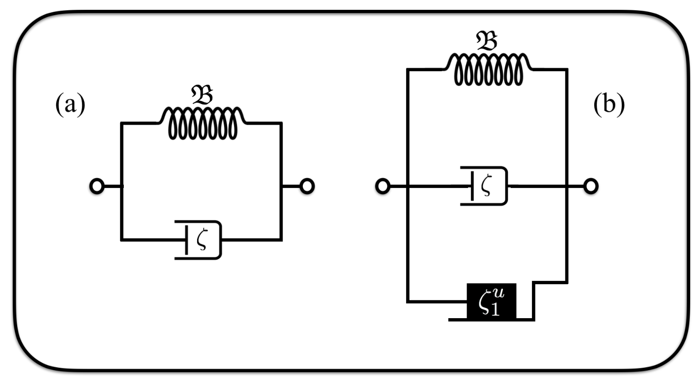
Refer to caption — Figure 1: Material diagrams for the bulk stresses sector of (a) Kelvin-Voigt model and (b) Bingham-Kelvin model. As all elements are connected in parallel (spring, dashpot and sliding frictional element) the total stress is given by the sum of each of the individual contributions.

Given the rheology equations (3.32), one can compare the constitutive relations found here with existent viscoelastic models. First of all, it should be noted that the last two lines in (3.4.1) describe several couplings between fluid and elastic degrees of freedom and a proper account of them in material models has not been considered in generality. Doing so requires introducing many new mechanical building blocks of the sliding frictional type. For simplicity, we consider the case in which $\mathfrak{P}=\eta^{u}_{1}=\eta_{2}^{u}=\zeta_{1}^{u}=\zeta_{2}^{u}=\bar{\zeta}^{u}=0$ which leads to the energy-momentum tensor

T^{\mu\nu}=\epsilon\,u^{\mu}u^{\nu}+P\,P^{\mu\nu}-\eta\,\sigma^{\mu\nu}-\zeta\,\Theta P^{\mu\nu}-2\mathfrak{G}\,\left(u^{\mu\nu}-\frac{1}{d}h^{\mu\nu}u^{\lambda}{}_{\!\!\lambda}\right)-\mathfrak{B}\,u^{\lambda}{}_{\!\!\lambda}\,h^{\mu\nu}\penalty\ \penalty\ .

(3.33)

This form of the stress tensor, together with (3.32), is known as the Kelvin-Voigt model and usually represented as in fig. 1(a), where we have focused on the bulk stresses sector (i.e. we have depicted the effect of bulk viscosity and bulk elastic modulus) and ignored the ideal fluid part.

Another model that illustrates the use of coupling terms between elastic and fluid degrees of freedom is the Bingham-Kelvin model for which $\mathfrak{P}=\eta^{u}_{1}=\eta_{2}^{u}=\zeta_{2}^{u}=\bar{\zeta}^{u}=0$ and the energy-momentum tensor becomes

T^{\mu\nu}=\epsilon\,u^{\mu}u^{\nu}+P\,P^{\mu\nu}-\zeta\,\Theta P^{\mu\nu}-\mathfrak{B}\,u^{\lambda}{}_{\!\!\lambda}\,h^{\mu\nu}-\zeta^{u}_{1}\,u^{\lambda}{}_{\!\!\lambda}\Theta P^{\mu\nu}\penalty\ \penalty\ ,

(3.34)

where we have ignored the shear contribution to the stresses. The last term in (3.34) is the term responsible for the frictional slide element (black box) depicted in fig. 1(b).

The entire possibility of linear responses (3.4.1) allows for more intricate and rich material diagrams. The full nonlinear theory of section 3.3 also allows for nonlinear responses to strain and hence for the description of non-Newtonian fluids. However, it is not capable of describing Maxwell-type models or Zener models as these violate the second condition in (3.32). Such models allow for plastic deformations and require that we consider a dynamical reference crystal metric $\mathbb{h}_{IJ}$ as in [7]. We intend to pursue this generalisation in the future.

3.5 Linearised fluctuations

In this section we study linearised fluctuations of equilibrium states of isotropic crystals. We consider crystals coupled to a flat background $g_{\mu\nu}=\eta_{\mu\nu}$ and vanishing external sources $K^{I}_{\text{ext}}=0$ , with static equilibrium configurations given by

u^{\mu}=\delta^{\mu}_{t}\penalty\ \penalty\ ,\penalty\ \penalty\ T=T_{0}\penalty\ \penalty\ ,\penalty\ \penalty\ \phi^{I}=x^{I}\penalty\ \penalty\ .

(3.35)

Note that in equilibrium we have $h^{IJ}=\bbdelta^{IJ}$ , corresponding to a crystal subjected to no strain. In general the system also admits solutions of the type $\phi^{I}=\alpha\,x^{I}$ corresponding to a uniform strain. Such configurations are allowed for a space filling crystal, but will need to be supplied with appropriate boundary conditions if the crystal was finite in extent. Since such configurations can be obtained by a trivial rescaling of $\phi^{I}$ ’s, we do not consider them here.

3.5.1 Modes

Let us consider small perturbation of the equilibrium state parametrised by

u^{\mu}=\delta^{\mu}_{t}+\delta u^{\mu}\quad\text{with}\quad\delta u^{t}=0\penalty\ \penalty\ ,\qquad T=T_{0}+\delta T\penalty\ \penalty\ ,\qquad\phi^{I}=x^{I}+\delta\phi^{I}\penalty\ \penalty\ .

(3.36)

Plugging in a plane wave ansatz and solving the equations of motion (3.15) linearly in the perturbations, we can find the solutions

$\displaystyle\delta u^{I}$	$\displaystyle=\left(1+\frac{(\omega^{2}+k^{2})\mathfrak{P}-k^{2}\left(\mathfrak{B}+2\frac{d-1}{d}\mathfrak{G}+\mathfrak{P}^{\prime 2}/s^{\prime}\right)}{i\omega\sigma}\right)k^{I}A_{\parallel}\mathrm{e}^{i(k_{I}x^{I}-\omega t)}$
	$\displaystyle\qquad+\left(1+\frac{\omega^{2}\mathfrak{P}-k^{2}\mathfrak{G}}{i\omega\sigma}\right)A_{\perp}^{I}\mathrm{e}^{i(k_{I}x^{I}-\omega t)}\penalty\ \penalty\ ,$
$\displaystyle\delta\phi^{I}$	$\displaystyle=\frac{i}{\omega}\left(1+\frac{k^{2}}{i\omega\sigma}\frac{Ts\,\mathfrak{P}^{\prime}}{s^{\prime}}\right)k^{I}A_{\parallel}\mathrm{e}^{i(k_{I}x^{I}-\omega t)}+\frac{i}{\omega}A^{I}_{\perp}\mathrm{e}^{i(k_{I}x^{I}-\omega t)}\penalty\ \penalty\ ,$
$\displaystyle\delta T$	$\displaystyle=\frac{k^{2}}{\omega}\left(\frac{s+\mathfrak{P}^{\prime}}{s^{\prime}}+\frac{(\omega^{2}+k^{2})\mathfrak{P}-\left(\mathfrak{B}+2\frac{d-1}{d}\mathfrak{G}\right)k^{2}}{i\omega\sigma s^{\prime}/s}\right)A_{\parallel}\mathrm{e}^{i(k_{I}x^{I}-\omega t)}\penalty\ \penalty\ .$	(3.37)

We have suppressed the arguments of various transport coefficients but they are understood to be evaluated on the equilibrium configuration. In addition, we have omitted the effect of viscosities but we consider it explicitly below. Primes denote a derivative with respect to temperature. We have also used the isotropy of the system to decompose

$\displaystyle\frac{\partial P}{\partial h^{IJ}}\bigg\|_{h=\alpha^{2}\bbdelta}$	$\displaystyle=-\frac{1}{2}\mathfrak{P}(T)\,\bbdelta_{IJ}\penalty\ \penalty\ ,$
$\displaystyle\frac{\partial P}{\partial h^{IJ}\partial h^{KL}}\bigg\|_{h=\alpha^{2}\bbdelta}$	$\displaystyle=\frac{1}{2}\left(\mathfrak{P}(T)-\mathfrak{G}(T)\right)\bbdelta_{I(L}\bbdelta_{K)J}-\frac{1}{4}\left(\mathfrak{B}(T)-\frac{2}{d}\mathfrak{G}(T)\right)\bbdelta_{IJ}\bbdelta_{KL}\penalty\ \penalty\ ,$
$\displaystyle\sigma_{IJ}\big\|_{h=\alpha^{2}\bbdelta}$	$\displaystyle=\sigma(T)\,\bbdelta_{IJ}\penalty\ \penalty\ ,$	(3.38)

using the same transport coefficients introduced in sec. 3.4.¹³¹³ 13 If we were to work around an equilibrium state with $\phi^{I}=\alpha x^{I}$ , we would get the same expressions, except that these coefficients will be defined around the new equilibrium state and will not have an interpretation in terms of linear transport coefficients. The symbols $A_{\parallel}$ and $A_{\perp}^{I}$ (with $A_{\perp}^{I}k_{I}=0$ ) denote arbitrary amplitudes corresponding to “longitudinal” and “transverse” modes respectively. The respective dispersion relations, in small momentum and frequency regime, are given by

$\displaystyle A_{\parallel}:\quad$	$\displaystyle\omega\left(\omega^{2}Ts-k^{2}\left(\frac{(s+\mathfrak{P}^{\prime})^{2}}{s^{\prime}}+\omega\frac{Ts}{i\sigma}\frac{\mathfrak{P}^{\prime 2}}{s^{\prime}}\right)\right)+i\omega^{2}k^{2}\left(\zeta+2\frac{d-1}{d}\eta\right)$
	$\displaystyle\qquad+\left(\omega+\frac{Ts}{i\sigma}\left(\omega^{2}-\frac{s}{Ts^{\prime}}k^{2}\right)\right)\left((\omega^{2}+k^{2})\mathfrak{P}-k^{2}\left(\mathfrak{B}+2\frac{d-1}{d}\mathfrak{G}\right)\right)=0\penalty\ \penalty\ ,$
$\displaystyle A_{\perp}:\quad$	$\displaystyle\omega^{2}sT+\left(1+\frac{\omega Ts}{i\sigma}\right)\left(\omega^{2}\mathfrak{P}-k^{2}\mathfrak{G}\right)+i\omega k^{2}\eta=0\penalty\ \penalty\ .$	(3.39)

Solving these equations, we find that in the longitudinal sector we have the usual sound mode along with a new diffusion mode characteristic of a lattice¹⁴¹⁴ 14 This diffusion mode was identified in [50] and in holographic setups in [35, 51, 36].

\omega(k)=\pm v_{\parallel}k-i\frac{\Gamma_{\parallel}}{2}k^{2}+\mathcal{O}(k^{3})\penalty\ \penalty\ ,\qquad\omega(k)=-iD_{\parallel}k^{2}+\mathcal{O}(k^{3})\penalty\ \penalty\ ,

(3.40)

where

	$\displaystyle v_{\parallel}^{2}=\frac{(s+\mathfrak{P}^{\prime})^{2}/s^{\prime}-\mathfrak{P}+\mathfrak{B}+2\frac{d-1}{d}\mathfrak{G}}{Ts+\mathfrak{P}}\penalty\ \penalty\ ,\qquad\Gamma_{\parallel}=\frac{T^{2}s^{2}v_{\parallel}^{2}}{\sigma(Ts+\mathfrak{P})}\left(1-\frac{s+\mathfrak{P}^{\prime}}{Ts^{\prime}v_{\parallel}^{2}}\right)^{2}+\frac{\zeta+2\frac{d-1}{d}\eta}{Ts+\mathfrak{P}}\penalty\ \penalty\ ,$
	$\displaystyle D_{\parallel}=\frac{s^{2}}{\sigma s^{\prime}}\frac{-\mathfrak{P}+\mathfrak{B}+2\frac{d-1}{d}\mathfrak{G}}{(Ts+\mathfrak{P})v_{\parallel}^{2}}\penalty\ \penalty\ .$		(3.41)

On the other hand, in the transverse sector we have another sound mode

\omega(k)=\pm v_{\perp}k-i\frac{\Gamma_{\perp}}{2}k^{2}+\mathcal{O}(k^{3})\penalty\ \penalty\ ,

(3.42)

where

v_{\perp}^{2}=\frac{\mathfrak{G}}{Ts+\mathfrak{P}}\penalty\ \penalty\ ,\qquad\Gamma_{\perp}=\frac{T^{2}s^{2}\mathfrak{G}}{\sigma(Ts+\mathfrak{P})^{2}}+\frac{\eta}{Ts+\mathfrak{P}}\penalty\ \penalty\ .

(3.43)

We see that the transverse sound mode is controlled by the shear modulus $\mathfrak{G}$ . On the other hand, the new diffusive mode is controlled by the transport coefficient $\sigma$ and $\eta$ . In the absence of the lattice pressure $\mathfrak{P}$ , these expressions simplify

	$\displaystyle v_{\parallel}^{2}=\frac{s}{Ts^{\prime}}+\frac{\mathfrak{B}+2\frac{d-1}{d}\mathfrak{G}}{Ts}\penalty\ ,\penalty\ \Gamma_{\parallel}=\frac{1}{\sigma Ts}\left(\mathfrak{B}+2\frac{d-1}{d}\mathfrak{G}\right)^{2}+\frac{\zeta+2\frac{d-1}{d}\eta}{Ts}\penalty\ ,\penalty\ D_{\parallel}=\frac{s}{\sigma Ts^{\prime}}\frac{\mathfrak{B}+2\frac{d-1}{d}\mathfrak{G}}{v_{\parallel}^{2}}\penalty\ \penalty\ ,$
	$\displaystyle v_{\perp}^{2}=\frac{\mathfrak{G}}{Ts}\penalty\ \penalty\ ,\qquad\Gamma_{\perp}=\frac{\mathfrak{G}}{\sigma}+\frac{\eta}{Ts}\penalty\ \penalty\ ,$		(3.44)

which might be more familiar to some readers.

For linear stability of the system, the imaginary part of $\omega(k)$ must be non-negative. This leads to the constraints $v_{\parallel}^{2},v_{\perp}^{2},\Gamma_{\parallel},\Gamma_{\perp},D_{\parallel}>0$ . In terms of coefficients, assuming that $Ts+\mathfrak{P}>0$ and the second law constraints $\eta,\zeta,\sigma\geq 0$ , we land on the parameter space

\frac{(s+\mathfrak{P}^{\prime})^{2}}{s^{\prime}}-\mathfrak{P}+\mathfrak{B}+2\frac{d-1}{d}\mathfrak{G}>0\penalty\ \penalty\ ,\qquad\mathfrak{G}>0\penalty\ \penalty\ ,\qquad\frac{-\mathfrak{P}+\mathfrak{B}+2\frac{d-1}{d}\mathfrak{G}}{s^{\prime}}>0\penalty\ \penalty\ .

(3.45)

On the other hand, for causality, we require $v_{\parallel}^{2},v_{\perp}^{2}<1$ . This leads to

\frac{(s+\mathfrak{P}^{\prime})^{2}}{s^{\prime}}-\mathfrak{P}+\mathfrak{B}+2\frac{d-1}{d}\mathfrak{G}<Ts+\mathfrak{P}\penalty\ \penalty\ ,\qquad\mathfrak{G}<Ts+\mathfrak{P}\penalty\ \penalty\ .

(3.46)

This gives the allowed range of parameters for a sensible evolution of the dynamical equations.

3.5.2 Linear response functions and Kubo formulas

We can extend the analysis above to read out the linear response functions of the theory by switching on plane wave background fluctuations. Let us start by setting $\sigma\to\infty$ and $\eta,\zeta\to 0$ turning off the dissipative corrections for simplicity. Let us take a perturbation of the background sources

g_{\mu\nu}=\eta_{\mu\nu}+\delta g_{\mu\nu}\penalty\ \penalty\ ,\qquad K^{\text{ext}}_{I}=\delta K^{\text{ext}}_{I}.

(3.47)

We can read out the solution of the equations of motion (3.15) by a straightforward computation

$\displaystyle\delta T$	$\displaystyle=\frac{s+\mathfrak{P}^{\prime}}{s^{\prime}\left(\omega^{2}-v_{\parallel}^{2}k^{2}\right)}\left(\left(2k^{2}v_{\perp}^{2}k^{JK}-\omega^{2}\bbdelta^{JK}\right)\frac{1}{2}\delta g_{JK}-\omega k^{J}\delta g_{tJ}-\frac{1}{2}k^{2}\delta g_{tt}-\frac{ik^{J}\delta K_{J}^{\text{ext}}}{Ts+\mathfrak{P}}\right)\penalty\ \penalty\ ,$
$\displaystyle\delta u^{I}$	$\displaystyle=\frac{\omega k^{I}}{\omega^{2}-v_{\parallel}^{2}k^{2}}\left(v_{\perp}^{2}k^{JK}\delta g_{JK}-\frac{\omega k^{J}}{k^{2}}\delta g_{tJ}-\frac{1}{2}\delta g_{tt}-v_{\parallel}^{2}\frac{1}{2}\bbdelta^{JK}\delta g_{JK}-\frac{ik^{J}/k^{2}\delta K_{J}^{\text{ext}}}{Ts+\mathfrak{P}}\right)$
	$\displaystyle\qquad-\omega\frac{\bbdelta^{IJ}-k^{I}k^{J}/k^{2}}{\omega^{2}-v_{\perp}^{2}k^{2}}\left(v_{\perp}^{2}k^{K}\delta g_{JK}+\omega\delta g_{tJ}+\frac{i\delta K^{\text{ext}}_{J}}{Ts+\mathfrak{P}}\right)\penalty\ \penalty\ ,$
$\displaystyle\delta\phi^{I}$	$\displaystyle=\frac{ik^{I}}{\omega^{2}-v_{\parallel}^{2}k^{2}}\left(v_{\perp}^{2}k^{JK}\delta g_{JK}-\frac{\omega k^{J}}{k^{2}}\delta g_{tJ}-\frac{1}{2}\delta g_{tt}-v_{\parallel}^{2}\frac{1}{2}\bbdelta^{JK}\delta g_{JK}-\frac{ik^{J}/k^{2}\delta K^{\text{ext}}_{J}}{Ts+\mathfrak{P}}\right)$
	$\displaystyle\qquad-i\frac{\bbdelta^{IJ}-k^{I}k^{J}/k^{2}}{\omega^{2}-v_{\perp}^{2}k^{2}}\left(v_{\perp}^{2}k^{K}\delta g_{JK}+\omega\delta g_{tJ}+\frac{i\delta K^{\text{ext}}_{J}}{Ts+\mathfrak{P}}\right)\penalty\ \penalty\ .$	(3.48)

The two point retarded Green’s functions are defined as

	$\displaystyle\mathcal{G}^{\mu\nu,\rho\sigma}_{TT,R}=-2\frac{\delta(\sqrt{-g}\,T^{\mu\nu})}{\delta g_{\rho\sigma}}\bigg\|_{\delta g=0,\delta K=0},\qquad\mathcal{G}^{I,J}_{\phi\phi,R}=\frac{\delta\phi^{I}}{\delta K_{J}^{\text{ext}}}\bigg\|_{\delta g=0,\delta K=0},$
	$\displaystyle\mathcal{G}^{I,\mu\nu}_{\phi T,R}=-2\frac{\delta\phi^{I}}{\delta g_{\mu\nu}}\bigg\|_{\delta g=0,\delta K=0}=\frac{\delta(\sqrt{-g}\,T^{\mu\nu})}{\delta K^{\text{ext}}_{I}}\bigg\|_{\delta g=0,\delta K=0}.$		(3.49)

Without loss of generality, we can choose the momentum to be in $k^{I}=\delta^{I}_{x}$ and denote the remaining spatial indices by $a,b,\ldots$ . Defining

\Delta_{\parallel}=\frac{\omega^{2}-v_{\parallel}^{2}k^{2}}{Ts+\mathfrak{P}}\penalty\ \penalty\ ,\qquad\Delta_{\perp}=\frac{\omega^{2}-v_{\perp}^{2}k^{2}}{Ts+\mathfrak{P}}\penalty\ \penalty\ ,

(3.50)

we read out the respective two point functions; in the longitudinal sector we have

	$\displaystyle\mathcal{G}^{tt,tt}_{TT,R}=\frac{k^{2}}{\Delta_{\parallel}}-\langle T^{tt}\rangle\penalty\ \penalty\ ,\qquad\mathcal{G}^{tt,tx}_{TT,R}=\frac{\omega k}{\Delta_{\parallel}}\penalty\ \penalty\ ,\qquad\mathcal{G}^{tt,xx}_{TT,R}=\frac{v_{\parallel}^{2}k^{2}}{\Delta_{\parallel}}+\langle T^{xx}\rangle\penalty\ \penalty\ ,\qquad\mathcal{G}^{tx,tx}_{TT,R}=\frac{v_{\parallel}^{2}k^{2}}{\Delta_{\parallel}}+\langle T^{tt}\rangle\penalty\ \penalty\ ,$
	$\displaystyle\mathcal{G}^{tx,xx}_{TT,R}=\frac{\omega kv_{\parallel}^{2}}{\Delta_{\parallel}}\penalty\ \penalty\ ,\qquad\mathcal{G}^{xx,xx}_{TT,R}=\frac{v_{\parallel}^{2}\omega^{2}}{\Delta_{\parallel}}+\langle T^{xx}\rangle\penalty\ \penalty\ ,$
	$\displaystyle\mathcal{G}^{x,xx}_{\phi T,R}=\frac{-ik}{(Ts+\mathfrak{P})\Delta_{\parallel}}\penalty\ \penalty\ ,\qquad\mathcal{G}^{x,tx}_{\phi T,R}=\frac{-i\omega}{(Ts+\mathfrak{P})\Delta_{\parallel}}\penalty\ \penalty\ ,\qquad\mathcal{G}^{x,tx}_{\phi T,R}=\frac{-i\omega^{2}/k}{(Ts+\mathfrak{P})\Delta_{\parallel}}+\frac{i}{k}\penalty\ \penalty\ ,$
	$\displaystyle\mathcal{G}^{x,x}_{\phi T,R}=\frac{-1}{(Ts+\mathfrak{P})^{2}\Delta_{\parallel}}\penalty\ \penalty\ .$		(3.51)

Similarly, in the transverse sector

	$\displaystyle\mathcal{G}^{tt,ab}_{TT,R}=\frac{k^{2}\left(v_{\parallel}^{2}-2v_{\perp}^{2}\right)}{\Delta_{\parallel}}\bbdelta^{ab}+\langle T^{ab}\rangle\penalty\ \penalty\ ,\qquad\mathcal{G}^{ta,tb}_{TT,R}=\left(\frac{v_{\perp}^{2}k^{2}}{\Delta_{\perp}}+\langle T^{tt}\rangle\right)\bbdelta^{ab}\penalty\ \penalty\ ,$
	$\displaystyle\mathcal{G}^{ab,cd}_{TT,R}=\left(\frac{k^{2}\left(v_{\parallel}^{2}-2v_{\perp}^{2}\right)^{2}}{\Delta_{\parallel}}+\frac{\left(s+\mathfrak{P}^{\prime}\right)^{2}}{s^{\prime}}+\mathfrak{B}-\mathfrak{P}\right)\bbdelta^{ab}\bbdelta^{cd}$
	$\displaystyle+\left(P+\mathfrak{P}\right)\left(2\delta^{c(a}\delta^{b)d}-\bbdelta^{ab}\bbdelta^{cd}\right)+2\mathfrak{G}\left(\delta^{c(a}\delta^{b)d}-\frac{1}{d}\bbdelta^{ab}\bbdelta^{cd}\right)\penalty\ \penalty\ ,$
	$\displaystyle\mathcal{G}^{a,tb}_{\phi T,R}=\frac{-i\omega}{(Ts+\mathfrak{P})\Delta_{\perp}}\bbdelta^{ab}\penalty\ \penalty\ ,\qquad\mathcal{G}^{a,b}_{\phi\phi,R}=\frac{-1}{(Ts+\mathfrak{P})^{2}\Delta_{\perp}}\bbdelta^{ab}\penalty\ \penalty\ .$		(3.52)

Finally, we have non-zero contributions in the cross sector

	$\displaystyle\mathcal{G}^{tx,ab}_{TT,R}=\frac{\omega k\left(v_{\parallel}^{2}-2v_{\perp}^{2}\right)}{\Delta_{\parallel}}\bbdelta^{ab}\penalty\ \penalty\ ,\qquad\mathcal{G}^{ta,xb}_{TT,R}=\frac{\omega kv_{\perp}^{2}}{\Delta_{\perp}}\bbdelta^{ab}\penalty\ \penalty\ ,$
	$\displaystyle\mathcal{G}^{xx,ab}_{TT,R}=\frac{\omega^{2}\left(v_{\parallel}^{2}-2v_{\perp}^{2}\right)}{\Delta_{\parallel}}\bbdelta^{ab}-\langle T^{ab}\rangle\penalty\ \penalty\ ,\qquad\mathcal{G}^{xa,xb}_{TT,R}=\frac{\omega^{2}v_{\perp}^{2}}{\Delta_{\perp}}\bbdelta^{ab}+\langle T^{ab}\rangle\penalty\ \penalty\ ,$
	$\displaystyle\mathcal{G}^{x,ab}_{\phi T,R}=\frac{ik\left(\frac{2\mathfrak{G}}{Ts+\mathfrak{P}}-v_{\parallel}^{2}\right)}{(Ts+\mathfrak{P})\Delta_{\parallel}}\bbdelta^{ab}\penalty\ \penalty\ .\qquad\mathcal{G}^{a,xb}_{\phi T,R}=\frac{i}{k}+\frac{-i\omega^{2}/k}{(Ts+\mathfrak{P})\Delta_{\perp}}\penalty\ \penalty\ .$		(3.53)

Note that all the correlators with odd number of transverse indices vanish due to isotropy

	$\displaystyle\mathcal{G}^{tt,ta}_{TT,R}=\mathcal{G}^{tx,ta}_{TT,R}=\mathcal{G}^{tt,xa}_{TT,R}=\mathcal{G}^{tx,xa}_{TT,R}=\mathcal{G}^{xx,xa}_{TT,R}=\mathcal{G}^{xx,ta}_{TT,R}=\mathcal{G}^{ta,bc}_{TT,R}=\mathcal{G}^{xa,bc}_{TT,R}=0\penalty\ \penalty\ ,$
	$\displaystyle\mathcal{G}^{x,ta}_{\phi T,R}=\mathcal{G}^{x,xa}_{\phi T,R}=\mathcal{G}^{a,tt}_{\phi T,R}=\mathcal{G}^{a,tx}_{\phi T,R}=\mathcal{G}^{a,xx}_{\phi T,R}=\mathcal{G}^{a,bc}_{\phi T,R}=0\penalty\ \penalty\ ,\qquad\mathcal{G}^{x,a}_{\phi\phi,R}=0\penalty\ \penalty\ .$		(3.54)

Upon turning on the dissipative transport coefficients, the two-point functions become much more involved. However, we report the respective Kubo formulas

	$\displaystyle\zeta+2\frac{d-1}{d}\eta=-\lim_{\omega\to 0}\lim_{k\to 0}\frac{\omega^{3}}{k^{4}}\mathrm{Im}\,G^{R}_{T^{tt}T^{tt}}\penalty\ \penalty\ ,\qquad\eta=-\lim_{\omega\to 0}\lim_{k\to 0}\frac{\omega}{k^{2}}\mathrm{Im}\,G^{R}_{T^{tx}T^{tx}}\penalty\ \penalty\ ,$
	$\displaystyle\frac{T^{2}s^{2}}{\sigma(Ts+\mathfrak{P})^{2}}=\lim_{\omega\to 0}\lim_{k\to 0}\omega\,\mathrm{Im}\,G^{R}_{\phi^{x}\phi^{x}}.$		(3.55)

These can be used to read out the transport coefficients in terms of linear responses functions.¹⁵¹⁵ 15 We would like to note that these Kubo formulas are different from the ones being used in [35] due to the presence of lattice pressure. The authors find a discrepancy between their numerical results from holography and those predicted by hydrodynamics. It seems quite plausible that this mismatch will be resolved upon taking into account the lattice pressure in the constitutive relations and Kubo formulas.

This finishes our quite detailed discussion of viscoelastic fluids. We have written down the most generic constitutive relations determining the dynamics of a viscoelastic fluid up to first order in the derivative expansion. In particular, we specialised to linear isotropic materials and obtained the respective constitutive relations, modes, and linear response functions. In the next section we present an equivalent formulation of viscoelasticity in terms of a fluid with partially broken higher-form symmetries.

4 $|$ Viscoelastic fluids as higher-form superfluids

In this section we present a formulation of hydrodynamics with partially broken generalised global symmetries and show their relation to the theory of viscoelastic fluids formulated in the previous section. Generalised global symmetries are an extension of ordinary global symmetries with one-form (vector) conserved currents and point-like conserved charges to higher-form conserved currents and higher dimensional conserved charges such as strings and branes [52]. It has been observed that when a fluid with a one-form symmetry¹⁶¹⁶ 16 A conserved $(k+1)$ -rank current $J^{\mu_{1}\ldots\mu_{k+1}}$ is said to be associated with a $k$ -form symmetry. Consequently, the ordinary global symmetries are zero-form in this language. has its symmetry partially broken along the direction of the fluid flow, it implements a symmetry-based reformulation of magnetohydrodynamics [24, 53, 26, 27]. In this section, we extend this partial symmetry breaking to hydrodynamics with multiple higher-form symmetries and show that the resultant theory is a dual description of viscoelastic fluids with translation broken symmetries in arbitrary dimensions. In $d$ spatial dimensions, one requires $d$ number of partially broken $(d-1)$ -form symmetries in order to describe viscoelasticity. The case of $d=2$ involving two one-form symmetries was considered in [22], albeit in a very restrictive case and ignoring the issues that require partial symmetry breaking. The understanding of partial symmetry breaking is essential for consistency of higher-form hydrodynamics with thermal equilibrium partition functions, as has been previously observed in [26, 25].

4.1 A dual formulation

In viscoelastic fluids with translation broken symmetries, all the dependence on the crystal field $\phi^{I}$ comes via its derivatives $e^{I}_{\mu}$ . As we have argued in section 3, the $\phi^{I}$ equations of motion can be used to eliminate $u^{\mu}e^{I}_{\mu}$ in favour of $P^{I\mu}=P^{\mu\nu}e^{I}_{\nu}$ and other constituent fields in the theory. Thus, it should be possible to reformulate the physics of viscoelastic fluids purely in terms of $P^{I\mu}$ and the hydrodynamic fields $u^{\mu}$ and $T$ , without referring to the microscopic fields $\phi^{I}$ .

To make this precise, we formally define a set of $d$ -form currents associated with the viscoelastic fluid by Hodge-dualising the derivatives of $\phi^{I}$ as

J^{I\mu_{1}\ldots\mu_{d}}[u^{\mu},T,P^{I\mu};g_{\mu\nu},K_{I}^{\text{ext}}]=\epsilon^{\mu\mu_{1}\ldots\mu_{d}}\partial_{\mu}\phi^{I}=\epsilon^{\mu\mu_{1}\ldots\mu_{d}}\left(P^{I}_{\mu}-Tu_{\mu}\delta_{\mathscr{B}}\phi^{I}\right)\penalty\ \penalty\ .

(4.1)

It is understood here that the $\phi^{I}$ equations of motion have been taken onshell to eliminate $\delta_{\mathscr{B}}\phi^{I}$ in terms of the remaining fields and background sources. Due to the symmetry of partial derivatives, these currents are conserved by construction

\nabla_{\mu_{1}}J^{I\mu_{1}\ldots\mu_{d}}=0\penalty\ \penalty\ .

(4.2)

A priori, these conservation equations have $d(d+1)/2$ independent components for every value of $I$ but only $d$ of these contain a time-derivative and hence govern dynamical evolution, while the remaining $d(d-1)/2$ components are constraints on an initial Cauchy slice. Conspicuously, these are the exact number of dynamical equations required to evolve the $d$ physical components in $P^{I\mu}$ for every value of $I$ (note that $u_{\mu}P^{I\mu}=0$ ).

The conservation equation (4.2) implies that there is a set of $d$ topological conserved charges $Q^{I}$ of the form

Q^{I}[\Sigma_{1}]=\int_{\Sigma_{1}}\star J^{I}\penalty\ \penalty\ ,

(4.3)

where $\Sigma_{1}$ is a given one-dimensional surface and $\star$ is the Hodge operator in $d+1$ dimensional spacetime. The charges $Q^{I}[\Sigma_{1}]$ count the number of lattice hyperplanes that intersect the one-dimensional surface $\Sigma_{1}$ .

The current (4.1) couples to the field strength of a higher-form gauge field. More precisely, we can replace the external currents $K_{I}^{\text{ext}}$ by the field strength such that

K_{I}^{\text{ext}}=-\frac{1}{(d+1)!}\epsilon^{\mu_{1}\ldots\mu_{d+1}}H_{I\mu_{1}\ldots\mu_{d+1}}\penalty\ \penalty\ .

(4.4)

Since $H_{I\mu_{1}\ldots\mu_{d+1}}$ is a full-rank form, locally it can be re-expressed as an exact form

H_{I\mu_{1}\ldots\mu_{d+1}}=(d+1)\partial_{[\mu_{1}}b_{I\mu_{2}\ldots\mu_{d+1}]}\penalty\ \penalty\ ,

(4.5)

where $b_{I\mu_{1}\ldots\mu_{d}}$ is a $d$ -form gauge field defined up to a $(d-1)$ -form gauge transformation

b_{I\mu_{1}\ldots\mu_{d}}\to b_{I\mu_{1}\ldots\mu_{d}}+d\,\partial_{[\mu_{1}}\Lambda_{I\mu_{2}\ldots\mu_{d}]}\penalty\ \penalty\ .

(4.6)

Using this definition, the energy-momentum conservation equation (3.1a) takes the form

\nabla_{\mu}T^{\mu\nu}=-K_{I}^{\text{ext}}\nabla^{\nu}\phi^{I}=\frac{1}{d!}H_{I}^{\nu\mu_{1}\ldots\mu_{d}}J^{I}_{\mu_{1}\ldots\mu_{d}}\penalty\ \penalty\ .

(4.7)

In essence, we have reformulated viscoelastic fluids in terms of a fluid with multiple $(d-1)$ -form global symmetries. The background $d$ -form gauge fields $b_{I\mu_{1}\ldots\mu_{d}}$ couple to the $d$ -form currents $J^{I\mu_{1}\ldots\mu_{d}}$ . The constitutive relations of viscoelastic fluids can be equivalently re-expressed as

T^{\mu\nu}[u^{\mu},T,P^{I\mu};g_{\mu\nu},b_{I\mu_{1}\ldots\mu_{d}}]\penalty\ \penalty\ ,\penalty\ \penalty\ J^{\mu_{1}\ldots\mu_{d}}_{I}[u^{\mu},T,P^{I\mu};g_{\mu\nu},b_{I\mu_{1}\ldots\mu_{d}}]\penalty\ \penalty\ .

(4.8)

The dynamics of the hydrodynamic fields $u^{\mu}$ and $T$ , and $P^{I\mu}$ is governed by energy-momentum conservation (4.7) and $d$ -form conservation equations (4.2).¹⁷¹⁷ 17 Note that, by the definition of the $d$ -form currents, we have the following relation $u_{\mu_{1}}J^{I\mu_{1}\ldots\mu_{d}}=\epsilon^{\mu\mu_{1}\ldots\mu_{d}}P^{I}_{\mu}u_{\mu_{1}}\penalty\ \penalty\ ,$ which can be understood as a frame choice from the higher-form hydrodynamic perspective. In general, we can choose a different set of fields in the hydrodynamic description which are aligned with $P_{I}^{\mu}$ in this particular frame, but can be arbitrarily redefined otherwise.

4.2 Formalities of higher-form hydrodynamics

4.2.1 Ordinary higher-form hydrodynamics

Having motivated a dual formulation of viscelastic fluids in terms of higher-form symmetries, we consider higher-form hydrodynamics in its own right, following [26, 25]. Consider a fluid living in $(d+1)$ -dimensions that carries a conserved energy-momentum tensor $T^{\mu\nu}$ and a $k$ number of conserved $d$ -form currents $J^{I\mu_{1}\ldots\mu_{d}}$ where $I=1,2,\ldots,k$ . When coupled to a background metric $g_{\mu\nu}$ and background $d$ -form gauge fields $b_{I\mu_{1}\ldots\mu_{d}}$ , the associated conservation equations are given as

\nabla_{\mu}T^{\mu\nu}=\frac{1}{d!}H_{I}^{\nu\mu_{1}\ldots\mu_{d}}J^{I}_{\mu_{1}\ldots\mu_{d}},\qquad\nabla_{\mu_{1}}J^{I\mu_{1}\ldots\mu_{d}}=0\penalty\ \penalty\ .

(4.9)

In a generic number of dimensions, the conservation equations lead to $(d+1+kd)$ dynamical equations and $kd(d-1)/2$ constraints. From this counting procedure, it can be checked that eqs. (4.9) can provide dynamics for a set of symmetry parameters

\mathscr{B}=\left(\beta^{\mu}\penalty\ ,\penalty\ \Lambda^{\beta}_{I\mu_{1}\ldots\mu_{d-1}}\right)\penalty\ \penalty\ .

(4.10)

Under an infinitesimal symmetry transformation parametrised by $\mathscr{X}=(\chi^{\mu},\Lambda^{\chi}_{I\mu_{1}\ldots\mu_{d-1}})$ , they transform according to

\delta_{\mathscr{X}}\beta^{\mu}=\pounds_{\chi}\beta^{\mu}\penalty\ \penalty\ ,\penalty\ \penalty\ \delta_{\mathscr{X}}\Lambda^{\beta}_{I\mu_{1}\ldots\mu_{d-1}}=\pounds_{\chi}\Lambda^{\beta}_{I\mu_{1}\ldots\mu_{d-1}}-\pounds_{\beta}\Lambda^{\chi}_{I\mu_{1}\ldots\mu_{d-1}}\penalty\ \penalty\ ,

(4.11)

where $\pounds_{\chi}$ denotes the Lie derivative with respect to $\chi^{\mu}$ . Let us repackage these fields into the fluid velocity $u^{\mu}$ , temperature $T$ , and $(d-1)$ -form chemical potentials $\mu_{I\mu_{1}\ldots\mu_{d-1}}$ according to

\frac{u^{\mu}}{T}=\beta^{\mu}\penalty\ \penalty\ ,\penalty\ \penalty\ \frac{\mu_{I\mu_{1}\ldots\mu_{d-1}}}{T}=\Lambda^{\beta}_{I\mu_{1}\ldots\mu_{d-1}}+\beta^{\nu}b_{I\nu\mu_{1}\ldots\mu_{d-1}}\penalty\ \penalty\ ,

(4.12)

such that $u^{\mu}u_{\mu}=-1$ . Interestingly, while the fields $u^{\mu}$ and $T$ are gauge invariant, $\mu_{I\mu_{1}\ldots\mu_{d-1}}$ transform akin to $(d-1)$ -form gauge fields

\mu_{I\mu_{1}\ldots\mu_{d-1}}\to\mu_{I\mu_{1}\ldots\mu_{d-1}}-(d-1)T\partial_{\mu_{1}}\left(\beta^{\nu}\Lambda_{I\nu\mu_{1}\ldots\mu_{d-1}}\right)\penalty\ \penalty\ .

(4.13)

Hence, they have the required $kd$ physical degrees of freedom, which, along with $u^{\mu}$ and $T$ , match the number of dynamical components of the conservation equations.

Similar to our discussion in section 3.1, higher-form fluids need to obey a version of the second law of thermodynamics. In the current context, this statement translates into the existence of an entropy current $S^{\mu}$ that satisfies

\nabla_{\mu}S^{\mu}+\frac{u_{\nu}}{T}\left(\nabla_{\mu}T^{\mu\nu}-\frac{1}{d!}H_{I}^{\nu\mu_{1}\ldots\mu_{d}}J^{I}_{\mu_{1}\ldots\mu_{d}}\right)-\frac{1}{(d-1)!}\frac{\mu_{I\mu_{1}\ldots\mu_{d-1}}}{T}\left(\nabla_{\mu}J^{I\mu\mu_{1}\ldots\mu_{d-1}}\right)=\Delta\geq 0\penalty\ \penalty\ .

(4.14)

Compared to eq. 3.2, here we have also taken into account the higher-form conservation equation and the respective multiplier has been chosen to be $\mu_{I\mu_{1}\ldots\mu_{d-1}}/T$ using the inherent redefinition freedom in the higher-form chemical potential. It is straightforward to formulate a higher-form analogue of the adiabaticity equation to ease the derivative of the constitutive relations. Defining the free energy current

N^{\mu}=S^{\mu}+\frac{1}{T}T^{\mu\nu}u_{\nu}-\frac{1}{(d-1)!}\frac{1}{T}J^{I\mu\mu_{1}\ldots\mu_{d-1}}\mu_{I\mu_{1}\ldots\mu_{d-1}}\penalty\ \penalty\ ,

(4.15)

the adiabaticity equation for higher-form fluids reads

\nabla_{\mu}N^{\mu}=\frac{1}{2}T^{\mu\nu}\delta_{\mathscr{B}}g_{\mu\nu}+\frac{1}{d!}J^{I\mu_{1}\ldots\mu_{d}}\delta_{\mathscr{B}}b_{I\mu_{1}\ldots\mu_{d}}+\Delta\penalty\ \penalty\ ,\penalty\ \penalty\ \Delta\geq 0\penalty\ \penalty\ .

(4.16)

We have identified the variations of the various background fields according to

\delta_{\mathscr{B}}g_{\mu\nu}=2\nabla_{(\mu}\beta_{\nu)}\penalty\ \penalty\ ,\penalty\ \penalty\ \delta_{\mathscr{B}}b_{I\mu_{1}\ldots\mu_{d}}=-d\,\partial_{[\mu_{1}}\left(\frac{1}{T}\mu_{I\mu_{2}\ldots\mu_{d}]}\right)+\beta^{\nu}H_{I\nu\mu_{1}\ldots\mu_{d}}\penalty\ \penalty\ .

(4.17)

To obtain the constitutive relations of a higher-form fluid, it is required to find the most generic expressions for $T^{\mu\nu}$ and $J^{I\mu_{1}\ldots\mu_{d}}$ in terms of the dynamical fields $u^{\mu}$ , $T$ , and $\mu_{I\mu_{1}\ldots\mu_{d-1}}$ , as well as background fields $g_{\mu\nu}$ and $b_{I\mu_{1}\ldots\mu_{d}}$ , arranged in a derivative expansion, that satisfy eq. 4.16 for some $N^{\mu}$ and $\Delta$ .

4.2.2 Partial symmetry breaking

When a higher-form symmetry is partially broken in its ground state, the hydrodynamic description should include the associated Goldstone modes $\varphi_{I\mu_{1}\ldots\mu_{d-2}}$ with $u^{\mu_{1}}\varphi_{I\mu_{1}\ldots\mu_{d-2}}=0$ , that transform according to¹⁸¹⁸ 18 If the $(d-1)$ -form symmetries were completely broken, we would instead introduce the $(d-1)$ -form Goldstone fields $\phi_{I\mu_{1}\ldots\mu_{d-1}}$ that shift under a background gauge transformation according to $\delta_{\mathscr{X}}\phi_{I\mu_{1}\ldots\mu_{d-1}}=\pounds_{\chi}\phi_{I\mu_{1}\ldots\mu_{d-1}}-\Lambda_{I\mu_{1}\ldots\mu_{d-1}}\penalty\ \penalty\ .$ The $(d-2)$ -form Goldstones of partial symmetry breaking are essentially the components of the full Goldstones along the direction of the fluid flow, that is $\varphi_{I\mu_{1}\ldots\mu_{d-2}}=\beta^{\mu}\phi_{I\mu\mu_{1}\ldots\mu_{d-2}}$ .

\delta_{\mathscr{X}}\varphi_{I\mu_{1}\ldots\mu_{d-2}}=\pounds_{\chi}\varphi_{I\mu_{1}\ldots\mu_{d-2}}-\beta^{\mu}\Lambda_{I\mu\mu_{1}\ldots\mu_{d-2}}.

(4.18)

This allows us to define a gauge-invariant version of the $(d-1)$ -form chemical potentials

\zeta_{I\mu_{1}\ldots\mu_{d-1}}=(d-1)\,T\partial_{[\mu_{1}}\varphi_{I\mu_{2}\ldots\mu_{d-1}]}-\mu_{I\mu_{1}\ldots\mu_{d-1}}\penalty\ \penalty\ .

(4.19)

The Goldstone fields are reminiscent of the crystal fields $\phi^{I}$ from sec. 3.1 and are accompanied by their own equations of motion, which can be schematically represented as

K^{I\mu_{1}\ldots\mu_{d-2}}=0\penalty\ \penalty\ .

(4.20)

As in the previous formulation, the operator $K^{I\mu_{1}\ldots\mu_{d-2}}$ is not predetermined without the knowledge of the microscopics but we can fix its form up to certain transport coefficients by imposing the second law of thermodynamics. In this context, this translates into the requirement that the fluid must admit an entropy current $S^{\mu}$ whose divergence must be positive-semi-definite in any arbitrary $\varphi_{I}$ -offshell configuration. Fixing the Lagrange multipliers associated with the respective conservation equations to be $\beta^{\mu}$ and $\zeta_{I\mu_{1}\ldots\mu_{d-1}}$ , the statement of the second can be written as

\nabla_{\mu}S^{\mu}+\frac{u_{\nu}}{T}\left(\nabla_{\mu}T^{\mu\nu}-\frac{1}{d!}H_{I}^{\nu\mu_{1}\ldots\mu_{d}}J^{I}_{\mu_{1}\ldots\mu_{d}}\right)\\ -\frac{1}{(d-1)!}\frac{\zeta_{I\mu_{1}\ldots\mu_{d-1}}}{T}\left(\nabla_{\mu}J^{I\mu\mu_{1}\ldots\mu_{d-1}}-(d-1)\,\beta^{\mu_{1}}K^{I\mu_{2}\ldots\mu_{d-1}}\right)=\Delta\geq 0\penalty\ \penalty\ ,

(4.21)

which is different than the corresponding statement in the symmetry unbroken phase given in (4.14). Defining the free energy current

N^{\mu}=S^{\mu}+\frac{1}{T}T^{\mu\nu}u_{\nu}-\frac{1}{(d-1)!}\frac{1}{T}J^{I\mu\mu_{1}\ldots\mu_{d-1}}\zeta_{I\mu_{1}\ldots\mu_{d-1}}\penalty\ \penalty\ ,

(4.22)

the associated adiabaticity equation becomes

\nabla_{\mu}N^{\mu}=\frac{1}{2}T^{\mu\nu}\delta_{\mathscr{B}}g_{\mu\nu}+\frac{1}{d!}J^{I\mu_{1}\ldots\mu_{d}}\delta_{\mathscr{B}}b_{I\mu_{1}\ldots\mu_{d}}+\frac{1}{(d-2)!}K^{I\mu_{1}\ldots\mu_{d-2}}\delta_{\mathscr{B}}\varphi_{I\mu_{1}\ldots\mu_{d-2}}+\Delta\penalty\ \penalty\ ,

(4.23)

with $\Delta\geq 0$ and where

\delta_{\mathscr{B}}\varphi_{I\mu_{1}\ldots\mu_{d-2}}=\frac{1}{T^{2}}u^{\mu}\zeta_{I\mu\mu_{1}\ldots\mu_{d-2}}\penalty\ \penalty\ .

(4.24)

Similar to section 3.1, we can use the leading order adiabaticity equation (4.23) to obtain the leading order version of the $\varphi_{I\mu_{1}\ldots\mu_{d-2}}$ equation of motion, namely

\delta_{\mathscr{B}}\varphi_{I\mu_{1}\ldots\mu_{d-2}}=\mathcal{O}(\partial)\qquad\implies\qquad u^{\mu_{1}}\zeta_{I\mu_{1}\ldots\mu_{d-1}}=\mathcal{O}(\partial)\penalty\ \penalty\ .

(4.25)

We can use some of the inherent redefinition freedom in $\mu_{I\mu_{1}\ldots\mu_{d-1}}$ to convert this into an exact all order statement. Consequently, it is possible to take $\varphi_{I\mu_{1}\ldots\mu_{d-2}}$ formally on-shell setting $\delta_{\mathscr{B}}\varphi_{I\mu_{1}\ldots\mu_{d-2}}=0$ , following which, the adiabaticity equation (4.23) turns into its “symmetry-unbroken” version (4.16). The constitutive relations of a higher-form fluid with partially broken symmetry are given by the most generic expressions for $T^{\mu\nu}$ and $J^{I\mu_{1}\ldots\mu_{d}}$ in terms of the dynamical fields $u^{\mu}$ , $T$ , and $\zeta_{I\mu_{1}\ldots\mu_{d-1}}$ (with $u^{\mu}u_{\mu}=-1$ and $u^{\mu_{1}}\zeta_{I\mu_{1}\ldots\mu_{d-1}}=0$ ), and background fields $g_{\mu\nu}$ and $b_{I\mu_{1}\ldots\mu_{d}}$ , arranged in a derivative expansion, that satisfy eq. 4.16 for some $N^{\mu}$ and $\Delta$ .

While $\zeta_{I\mu_{1}\ldots\mu_{d-1}}$ is fundamentally more transparent, for most of the explicit computations, it will be helpful to work with a Hodge-dualised version

\psi^{\mu}_{I}=\frac{1}{(d-1)!}\epsilon^{\mu\mu_{1}\ldots\mu_{d}}u_{\mu_{1}}\zeta_{I\mu_{2}\ldots\mu_{d}}\penalty\ \penalty\ ,\penalty\ \zeta_{I\mu_{1}\ldots\mu_{d-1}}=\epsilon_{\mu\nu\mu_{1}\ldots\mu_{d-1}}\psi_{I}^{\mu}u^{\nu}\penalty\ \penalty\ ,

(4.26)

where we note that $u_{\mu}\psi_{I}^{\mu}=0$ . This representation makes it clear that $\psi_{I}^{\mu}$ , and hence $\zeta_{I\mu_{1}\ldots\mu_{d-1}}$ , have the same degrees of freedom as $P^{I\mu}$ and can be used as a fundamental hydrodynamic field for viscoelastic fluids instead. The relation between the two is typically non-trivial and needs to be obtained order-by-order in the derivative expansion.

Compared to eq. 3.4, the adiabaticity equation (4.16) in the dual formulation does not exhibit order mixing, as both $\delta_{\mathscr{B}}g_{\mu\nu}$ and $\delta_{\mathscr{B}}b_{I\mu_{1}\ldots\mu_{d}}$ are $\mathcal{O}(\partial)$ . This allows for a more transparent analysis of the constitutive relations, as we shall see in the next section. Another benefit of working in the dual formulation is that we directly obtain the constitutive relations for (the Hodge dual of) the physically observable crystal momenta, rather than for the equations of motion of the crystal fields. This can considerably simplify the computation of the respective correlation functions and Kubo formulae, as in the case of magnetohydrodynamics [25].

4.3 Revisiting ideal viscoelastic fluids

The constitutive relations of an ideal viscoelastic fluid in higher-form language are characterised by an ideal order free energy current

N^{\mu}=p(T,\gamma_{IJ})\,\beta^{\mu}+\mathcal{O}(\partial)\penalty\ \penalty\ .

(4.27)

Here $p(T,\gamma_{IJ})$ is an arbitrary function of all the available ideal order scalars in the theory, namely the temperature $T$ and matrix

\gamma_{IJ}=\frac{1}{(d-1)!}\zeta_{I\mu_{1}\ldots\mu_{d-1}}\zeta_{I\nu_{1}\ldots\nu_{d-1}}g^{\mu_{1}\nu_{1}}\ldots g^{\mu_{d-1}\nu_{d-1}}=\psi^{\mu}_{I}\psi^{\nu}_{J}g_{\mu\nu}\penalty\ \penalty\ .

(4.28)

Introducing this into eq. 4.16 and noting that¹⁹¹⁹ 19 Note that $\zeta_{I}{}^{\mu}{}_{\mu_{2}\ldots\mu_{d-1}}\zeta_{J}^{\nu\mu_{2}\ldots\mu_{d-1}}=(d-2)!(\gamma_{IJ}P^{\mu\nu}-\psi_{I}^{\nu}\psi_{J}^{\mu})$ .

\delta_{\mathscr{B}}\gamma_{IJ}=-\frac{2}{(d-1)!}u^{\mu_{1}}\zeta_{(I}^{\mu_{2}\ldots\mu_{d}}\delta_{\mathscr{B}}b_{J)\mu_{1}\ldots\mu_{d}}+\left(\psi^{\mu}_{I}\psi_{J}^{\nu}-\gamma_{IJ}g^{\mu\nu}\right)\delta_{\mathscr{B}}g_{\mu\nu}\penalty\ ,

(4.29)

we obtain the ideal viscoelastic fluid constitutive relations²⁰²⁰ 20 In [25], we have given a formulation of higher-form hydrodynamics with a single conserved current. In app. C.3 we provide the comparison between the ideal order higher-form hydrodynamics of this section with that of [25].

	$\displaystyle T^{\mu\nu}$	$\displaystyle=\left(\epsilon+p\right)u^{\mu}u^{\nu}+pg^{\mu\nu}-\frac{q^{IJ}}{(d-2)!}\zeta_{I}^{\mu}{}_{\mu_{2}\ldots\mu_{d-1}}\zeta_{J}^{\nu\mu_{2}\ldots\mu_{d-1}}+\mathcal{O}(\partial)\penalty\ \penalty\ ,$
	$\displaystyle J^{I\mu_{1}\ldots\mu_{d}}$	$\displaystyle=-d\,q^{IJ}u^{[\mu_{1}}\zeta_{J}^{\mu_{2}\ldots\mu_{d}]}+\mathcal{O}(\partial)\penalty\ \penalty\ .$		(4.30)

Here we have defined

\mathrm{d}p=s\mathrm{d}T+\frac{1}{2}q^{IJ}\mathrm{d}\gamma_{IJ}\penalty\ \penalty\ ,\penalty\ \penalty\ \epsilon+p=sT+q^{IJ}\gamma_{IJ}\penalty\ \penalty\ .

(4.31)

These are the most generic constitutive relations of an ideal viscoelastic fluid in higher-form language. As promised earlier, there is no order-mixing across derivative orders in this formulation. It is useful to explicitly work out the equations of motion for ideal viscoelastic fluids, which result in

	$\displaystyle\nabla_{\mu}(su^{\mu})=0\penalty\ \penalty\ ,$
	$\displaystyle\left(sTP^{\nu\mu}+q^{IJ}\psi^{\nu}_{J}\psi^{\mu}_{I}\right)u^{\lambda}\delta_{\mathscr{B}}g_{\mu\lambda}+\frac{1}{d!}q^{IJ}\psi^{\nu}_{J}\epsilon^{\mu\mu_{1}\ldots\mu_{d}}u_{\mu}\delta_{\mathscr{B}}b_{I\mu_{1}\ldots\mu_{d}}=0\penalty\ \penalty\ ,$
	$\displaystyle\nabla_{[\mu}\left(q^{IJ}\psi_{J\nu]}\right)=0\penalty\ \penalty\ .$		(4.32)

In order to find the relation between the two formalisms, we need to perform the identification according to eq. 4.1, which results in the following map between formulations

e^{I}_{\mu}=q^{IJ}\psi_{J\mu}+\mathcal{O}(\partial)\qquad\implies\qquad h^{IJ}=q^{IK}q^{JL}\gamma_{KL}+\mathcal{O}(\partial)\penalty\ \penalty\ .

(4.33)

Additionally, introducing this into the energy-momentum tensor, we find

	$\displaystyle p=P-r_{IJ}h^{IJ}+\mathcal{O}(\partial)\penalty\ \penalty\ ,\penalty\ \penalty\$
	$\displaystyle q^{IJ}=-q^{IK}q^{JK}r_{KL}\implies q^{IJ}=-(r^{-1})^{IJ}\penalty\ \penalty\ ,$		(4.34)

while temperature, entropy density and energy density agree in both formulations.

4.4 One derivative corrections

Following the same arguments as the previous subsection, we consider the hydrostatic free energy density in the dual picture

\mathcal{N}=p+\tilde{f}_{1}^{I}\frac{1}{T}\psi_{I}^{\mu}\partial_{\mu}T+2T\tilde{f}_{2}^{[IJ]}\psi_{I}^{\mu}\psi_{J}^{\nu}\partial_{[\mu}u_{\nu]}+\tilde{f}_{3}^{I(JK)}\psi_{I\mu}\partial_{\mu}\gamma_{JK}\penalty\ \penalty\ .

(4.35)

The hydrostatic constitutive relations can be obtained using the variations given above and refer the reader to appendix B for details. In turn, in the non-hydrostatic sector, we can expand

T^{\mu\nu}_{\text{nhs}}=\psi_{I}^{\mu}\psi_{J}^{\nu}\mathcal{T}^{IJ}\penalty\ \penalty\ ,\penalty\ \penalty\ J^{I\mu_{1}\ldots\mu_{d}}_{\text{nhs}}=\epsilon^{\mu\mu_{1}\ldots\mu_{d}}u_{\mu}\mathcal{J}^{I}\penalty\ .

(4.36)

The most general non-hydrostatic constitutive relations are correspondingly

\begin{pmatrix}\mathcal{T}^{IJ}\\ \mathcal{J}^{I}\end{pmatrix}=-T\begin{pmatrix}\tilde{\eta}^{IJKL}&\tilde{\chi}^{IJK}\\ \tilde{\chi}^{\prime IKL}&\tilde{\sigma}^{IK}\end{pmatrix}\begin{pmatrix}\frac{1}{2}\psi_{K}^{\mu}\psi_{L}^{\nu}\delta_{\mathscr{B}}g_{\mu\nu}\\ \frac{1}{d!}\epsilon^{\mu\mu_{1}\dots\mu_{d}}u_{\mu}\delta_{\mathscr{B}}b_{K\mu_{1}\ldots\mu_{d}}\end{pmatrix}\penalty\ \penalty\ .

(4.37)

The transport coefficient matrices have necessary symmetry properties. The positivity constraint requires that the symmetric part of the $5\times 5$ transport coefficient matrix is positive semi-definite.

In order to provide the map of transport coefficients at first order between the two formulations, we first use the identification in eq. 4.1 in order to obtain

P^{I}_{\mu}=\frac{1}{(d-1)!}\epsilon_{\mu\mu_{1}\ldots\mu_{d}}u^{\mu_{1}}u_{\nu}J^{I\nu\mu_{2}\ldots\mu_{d}}\penalty\ \penalty\ ,\penalty\ \penalty\ u^{\mu}\partial_{\mu}\phi^{I}=-\frac{1}{d!}\epsilon_{\mu\mu_{1}\ldots\mu_{d}}u^{\mu}J^{I\mu_{1}\ldots\mu_{d}}\penalty\ \penalty\ .

(4.38)

This provides a definition of $P_{I}^{\mu}$ and $\delta_{\mathscr{B}}\phi^{I}$ in the conventional formulation in terms of the dual formulation variables

$\displaystyle P^{I\mu}$	$\displaystyle=\left[q^{IJ}+\frac{2}{T}\frac{\partial\tilde{f}_{1}^{K}}{\partial\gamma_{IJ}}\psi_{K}^{\lambda}\partial_{\lambda}T+4T\frac{\partial\tilde{f}_{2}^{[KL]}}{\partial\gamma_{IJ}}\psi^{\rho}_{K}\psi^{\sigma}_{L}\partial_{[\rho}u_{\sigma]}+2\frac{\partial\tilde{f}_{3}^{L(MK)}}{\partial\gamma_{IJ}}\psi^{\lambda}_{L}\partial_{\lambda}\gamma_{MK}-2\nabla_{\rho}\left(\tilde{f}_{3}^{K(IJ)}\psi^{\rho}_{K}\right)\right]\psi^{\mu}_{J}$
	$\displaystyle\qquad+\tilde{f}_{1}^{I}\frac{1}{T}P^{\mu\nu}\partial_{\nu}T+4T\tilde{f}_{2}^{[IJ]}P^{\mu\nu}\psi^{\rho}_{J}\partial_{[\nu}u_{\rho]}+\tilde{f}_{3}^{I(JK)}P^{\mu\nu}\partial_{\nu}\gamma_{JK}\penalty\ \penalty\ ,$
$\displaystyle\delta_{\mathscr{B}}\phi^{I}$	$\displaystyle=\tilde{\chi}^{\prime IKL}\frac{1}{2}\psi_{K}^{\mu}\psi_{L}^{\nu}\delta_{\mathscr{B}}g_{\mu\nu}+\tilde{\sigma}^{IK}\frac{1}{d!}\epsilon^{\mu\mu_{1}\dots\mu_{d}}u_{\mu}\delta_{\mathscr{B}}b_{K\mu_{1}\ldots\mu_{d}}.$	(4.39)

We wish to begin the comparison with the free energy currents in the two formulations. Using eq. 4.15, we know that

N^{\mu}=N^{\mu}_{\text{elastic}}+\frac{u^{\mu}}{T}\psi^{I\nu}P_{I\nu}-\psi^{I\mu}\delta_{\mathscr{B}}\phi_{I}\penalty\ \penalty\ .

(4.40)

Using the map (4.4) and the results from appendix B, we infer the map between the hydrostatic transport coefficients

	$\displaystyle p(T,\gamma_{IJ})=P(T,q^{IK}q^{JL}\gamma_{KL})+q^{IJ}\gamma_{IJ}\penalty\ \penalty\ ,$
	$\displaystyle\tilde{f}_{1}^{I}=f^{1}_{J}q^{JI}+2Tq^{IM}q^{JN}\gamma_{NL}\frac{\partial q^{KL}}{\partial T}f^{3}_{M(JK)}\penalty\ \penalty\ ,$
	$\displaystyle\tilde{f}_{2}^{[IJ]}=f^{2}_{[MN]}q^{MI}q^{NJ}\penalty\ \penalty\ ,$
	$\displaystyle\tilde{f}_{3}^{I(JK)}=f^{3}_{N(LM)}q^{IN}q^{JL}q^{KM}+2q^{IM}q^{AN}\gamma_{NL}\frac{\partial q^{BL}}{\partial\gamma_{JK}}f^{3}_{M(AB)}\penalty\ \penalty\ .$		(4.41)

To obtain the map in the non-hydrostatic sector, we need to compare the energy-momentum tensors and $\delta_{\mathscr{B}}\phi^{I}$ in the two formulations. In hindsight, we allow for a relative field redefinition of the fluid velocity between the two formulations, i.e $u^{\mu}_{\text{elastic}}=u^{\mu}+\delta u^{\mu}$ with $u_{\mu}\delta u^{\mu}=0$ . The $\varphi^{I}$ -equation of motion (3.22), upon using the said field redefinition, implies that

	$\displaystyle\sigma_{IJ}\delta_{\mathscr{B}}\phi^{J}+\frac{1}{T}\sigma_{IJ}e^{J}_{\lambda}\delta u^{\lambda}$	$\displaystyle=\frac{1}{T}\bigg(K_{J}^{\text{ext}}-\nabla_{\mu}\left(r_{JK}e^{K\mu}\right)-\chi^{\prime}_{JKL}P^{K\mu}P^{L\nu}\nabla_{(\mu}u_{\nu)}\bigg)$
		$\displaystyle=\left(\frac{1}{d!}\epsilon^{\lambda\mu_{1}\ldots\mu_{d}}u_{\lambda}\delta_{\mathscr{B}}b_{I\mu_{1}\ldots\mu_{d}}-\frac{1}{2}\chi^{\prime}_{IMN}q^{MK}q^{NL}\psi^{\mu}_{K}\psi^{\nu}_{K}\delta_{\mathscr{B}}g_{\mu\nu}\right).$		(4.42)

On the other hand, using the results from appendix B, it is straight-forward, albeit cumbersome, to obtain that

T^{\mu\nu}_{\text{elastic,hs}}=T^{\mu\nu}_{\text{hs}}+2Tu^{(\mu}\left(s\delta u^{\nu)}-\psi^{\nu)}_{I}\delta_{\mathscr{B}}\phi^{I}\right).

(4.43)

Given that all the non-hydrostatic corrections are in the Landau frame, we must choose the velocity field-redefinition to be $\delta u^{\mu}=\psi^{\mu}_{I}\delta_{\mathscr{B}}\phi^{I}/s$ , mapping the hydrostatic sectors of the two formulations to each other. Comparing $\delta_{\mathscr{B}}\phi^{J}$ from section 4.4 to section 4.4 and comparing the non-hydrostatic energy-momentum tensors in the two formulations, we obtain the map

	$\displaystyle\tilde{\eta}^{IJKL}=q^{IA}q^{JB}q^{KC}q^{LD}\left(\eta_{ABCD}-\chi_{ABR}\tilde{\sigma}^{RS}\chi^{\prime}_{SCD}\right)\penalty\ \penalty\ ,$
	$\displaystyle\tilde{\chi}^{IJK}=q^{IA}q^{JB}\chi_{ABC}\tilde{\sigma}^{CK}\penalty\ \penalty\ ,$
	$\displaystyle\tilde{\chi}^{\prime IJK}=-\tilde{\sigma}^{IL}\chi^{\prime}_{LMN}q^{JM}q^{KN}\penalty\ \penalty\ ,$
	$\displaystyle(\tilde{\sigma}^{-1})_{IJ}=\sigma_{IJ}+\frac{\sigma_{IK}}{Ts}q^{KL}\gamma_{LJ}\penalty\ \penalty\ .$		(4.44)

This completes the formulation of viscoelastic hydrodynamics in terms of generalised global symmetries and shows that it can exactly accommodate viscoelastic hydrodynamics with broken translation invariance. In the next section we look at particular realisations of both these formulations in the context of holography.

5 $|$ Conformal viscoelastic fluids and holography

In this section we provide, and study the properties of, holographic models in $D=4,5$ bulk dimensions (i.e. $d=2,3$ spatial dimensional fluids). The models we consider in general break conformal symmetry due to double trace deformations but conformal symmetry can be recovered in a specific case. Thus, in the beginning of this section we consider conformal fluids. In connection with viscoelastic holography, we consider two classes of models that have been considered in the literature. The first class of models has translation broken symmetries involving a set of $(D-2)$ scalar fields $\Phi_{I}$ minimally coupled to gravity. The second class is formulated in the context of generalised global symmetries and involve a set of $(D-2)$ gauge fields $B_{Ia_{1}...a_{D-2}}$ minimally coupled to gravity [22]. The latter class describes particular equilibrium states of the higher-form hydrodynamics described in sec. 4, which we explicitly show by generalising the work of [22] to $D=5$ . Given that in this case the dual fluid is governed by conservation equations alone (i.e. no dynamical fields), which has been one of the motivations in the holographic digressions of [54, 55, 22], we consider it first. Later, generalising aspects of [56], we “dualise” the model with higher-form symmetries and obtain the class of viscoelastic models with translation broken symmetries, which consist of the model of [39] but with an alternative quantisation of the scalar fields and a double trace deformation of the boundary theory. We show that this process results in the dual fluid given in section 3.

5.1 Conformal viscoelastic fluids

A viscoelastic fluid is said to be conformal if it is invariant under the conformal rescaling of the background metric $g_{\mu\nu}\to\Omega^{2}g_{\mu\nu}$ for some arbitrary function $\Omega(x)$ . In practice, it implies that the energy-momentum tensor of the theory is traceless (modulo conformal anomalies) and the constitutive relations are only constructed out of the conformal covariants.

5.1.1 Constitutive relations

Focusing on the non-anomalous case, setting the trace of the energy-momentum tensor (3.3) to zero, we get certain constraints on the respective transport coefficients, namely

	$\displaystyle\epsilon=d\,P-r_{IJ}h^{IJ},\qquad f^{1}_{I}=f^{3}_{I(JK)}=0\penalty\ \penalty\ ,\qquad(d-3)f^{2}_{[IJ]}-T\frac{\partial f^{2}_{[IJ]}}{\partial T}-2h^{KL}\frac{\partial f^{2}_{[IJ]}}{\partial h^{KL}}=0\penalty\ \penalty\ ,$
	$\displaystyle h^{IJ}\eta_{IJKL}=h^{IJ}\chi_{IJK}=0\penalty\ \penalty\ .$	(5.1a)
Furthermore, requiring $T^{\mu\nu}$ and $K_{I}$ to only involve conformal covariants requires
	$\eta_{IJKL}h^{KL}=\chi^{\prime}_{IKL}h^{KL}=0\penalty\ \penalty\ .$	(5.1b)

The first equation in eq. 5.1 determines the energy density in conformal fluids as expected. At the one-derivative hydrostatic order, we see that we are only left with $f^{2}_{[IJ]}$ which is the only conformal covariant term in the free-energy current. In the non-hydrostatic sector, we essentially just eliminate the conformal-non-invariant $\nabla_{\mu}u^{\mu}$ term from the constitutive relations. Consequently we get

	$\displaystyle T^{\mu\nu}_{\text{conformal}}$	$\displaystyle=(\epsilon+P)u^{\mu}u^{\nu}+Pg^{\mu\nu}-r_{IJ}e^{I\mu}e^{J\nu}+T^{\langle\mu\nu\rangle}_{f_{2}}$
		$\displaystyle\qquad-P^{I\langle\mu}P^{J\nu\rangle}\eta_{IJKL}P^{K\langle\rho}P^{L\sigma\rangle}\nabla_{\rho}u_{\sigma}-P^{I\langle\mu}P^{J\nu\rangle}\chi_{IJK}u^{\rho}\partial_{\rho}\phi^{K}+\mathcal{O}(\partial^{2})\penalty\ \penalty\ ,$		(5.2)

and

u^{\mu}\partial_{\mu}\phi^{I}\big|_{\text{conformal}}=(\sigma^{-1})^{IJ}\left[K_{J}^{\text{ext}}-\nabla_{\mu}\left(r_{JK}e^{K\mu}\right)-\chi^{\prime}_{JKL}P^{K\langle\mu}P^{L\nu\rangle}\nabla_{\mu}u_{\nu}\right]+\mathcal{O}(\partial^{2})\penalty\ \penalty\ .

(5.3)

We will now focus on a special case of these constitutive relations.

5.1.2 Linear conformal isotropic materials

For conformal viscoelastic fluids truncated to linear order in strain, we need to additionally impose the constraints (5.1) on top of the constitutive relations section 3.4.1, leading to

T\partial_{T}P_{\text{f}}=(d+1)\,P_{\text{f}}+d\,\mathfrak{P}\penalty\ \penalty\ ,\penalty\ \penalty\ T\partial_{T}\mathfrak{P}=(d+1)\,\mathfrak{P}-d\,\mathfrak{B}\penalty\ \penalty\ ,\penalty\ \penalty\ \zeta=\zeta^{u}_{1}=\zeta^{u}_{2}=\bar{\zeta}^{u}=0\penalty\ \penalty\ .

(5.4)

This gives the following constitutive relations of a linear conformal viscoelastic fluid

$\displaystyle T^{\mu\nu}$	$\displaystyle=(d+1)\,P_{\text{f}}\,u^{\mu}u^{\nu}+P_{\text{f}}\,g^{\mu\nu}-\eta\,\sigma^{\mu\nu}$
	$\displaystyle\qquad+T\partial_{T}\mathfrak{P}\,u^{\lambda}{}_{\!\!\lambda}\left(u^{\mu}u^{\nu}+\frac{1}{d}h^{\mu\nu}\right)+\mathfrak{P}\,\left(d\,u^{\mu}u^{\nu}+h^{\mu\nu}+u^{\lambda}{}_{\!\!\lambda}\left(g^{\mu\nu}-\frac{d+1}{d}h^{\mu\nu}\right)\right)$
	$\displaystyle\qquad-2\mathfrak{G}\,\left(u^{\mu\nu}-\frac{1}{k}h^{\mu\nu}u^{\lambda}{}_{\!\!\lambda}\right)-\eta^{u}_{1}\,u^{\lambda}{}_{\!\!\lambda}\sigma^{\mu\nu}-\eta^{u}_{2}\left(u^{(\mu}{}_{\!\sigma}\sigma^{\nu)\sigma}-\frac{1}{d}P^{\mu\nu}u_{\rho\sigma}\sigma^{\rho\sigma}\right)+\mathcal{O}(u^{2})\penalty\ \penalty\ ,$	(5.5)

while the $\phi^{I}$ equation of motion is still given by section 3.4.1. In the special case that the internal pressure of the lattice $\mathfrak{P}=0$ , we infer that the bulk modulus $\mathfrak{B}=0$ and these constitutive relations, along with the $\phi^{I}$ equations of motion (3.4.1), simplify to

$\displaystyle T^{\mu\nu}_{\text{conformal}}$	$\displaystyle=(d+1)\,P_{\text{f}}\,u^{\mu}u^{\nu}+P_{\text{f}}\,g^{\mu\nu}-\eta\,\sigma^{\mu\nu}$
	$\displaystyle\qquad-2\mathfrak{G}\,\left(u^{\mu\nu}-\frac{1}{k}h^{\mu\nu}u^{\lambda}{}_{\!\!\lambda}\right)-\eta^{u}_{1}\,u^{\lambda}{}_{\!\!\lambda}\sigma^{\mu\nu}-\eta^{u}_{2}\left(u^{(\mu}{}_{\!\sigma}\sigma^{\nu)\sigma}-\frac{1}{d}P^{\mu\nu}u_{\rho\sigma}\sigma^{\rho\sigma}\right)+\mathcal{O}(u^{2})\penalty\ \penalty\ ,$
$\displaystyle u^{\mu}\partial_{\mu}\phi^{I}\big\|_{\text{conformal}}$	$\displaystyle=\frac{1}{\sigma}h^{IJ}\left[K_{J}^{\text{ext}}-\nabla_{\mu}\left(2\mathfrak{G}\left(u_{JK}-\frac{1}{k}h_{JK}u^{\lambda}{}_{\!\!\lambda}\right)e^{K\mu}\right)\right]$
	$\displaystyle\qquad-\frac{1}{\sigma^{2}}\left(\sigma^{u}_{1}\,u^{\lambda}{}_{\!\!\lambda}h^{IJ}+\sigma^{u}_{2}\,u^{IJ}\right)K_{J}^{\text{ext}}+\mathcal{O}(u^{2})\penalty\ \penalty\ .$	(5.6)

The first line of the energy-momentum tensor represents the constitutive relations for an ordinary uncharged conformal fluid. The second line has the expected shear modulus term along with the variants of shear viscosities $\eta^{u}_{1}$ , $\eta^{u}_{2}$ representing the coupling of the conformal fluid to the strain of the crystal.

We would like to note that the constitutive relations (5.1.2) are, in principle, different from the ones obtained in [8]. The strain $u_{\mu\nu}$ defined in eq. 2.4 transforms inhomogeneously under a conformal transformation, i.e. $u_{\mu\nu}\to\Omega^{2}u_{\mu\nu}+\frac{1}{2}\left(\Omega^{2}-1\right)\mathbb{h}_{\mu\nu}$ , because conformal rescaling only acts on the physical distances and not on the reference distances between the crystal cores. It follows that the transport coefficients $\mathfrak{P}(T)$ , $\mathfrak{G}(T)$ , and $\eta^{u}_{1,2}(T)$ appearing in section 5.1.2 do not have a homogeneous conformal scaling. This is in contrast to [8], which chooses the conformal transformations to scale the reference metric as well, i.e. $\mathbb{h}_{IJ}\to\Omega^{2}\mathbb{h}_{IJ}$ , leading to a homogeneous scaling of the strain tensor $u_{\mu\nu}\to\Omega^{2}u_{\mu\nu}$ . In turn, the coefficients $\mathfrak{P}(T)$ , $\mathfrak{G}(T)$ , and $\eta^{u}_{1,2}(T)$ will all scale homogeneously. With this alternative choice, however, invariance of the partition function under conformal transformations does not agree with a traceless energy-momentum tensor. To wit,

-\delta_{\Omega}\ln\mathcal{Z}=\frac{1}{2}\Omega^{2}g_{\mu\nu}\langle T^{\mu\nu}\rangle-\Omega^{2}\mathbb{h}_{IJ}(\delta\ln\mathcal{Z}/\delta\mathbb{h}_{IJ})=0\qquad\implies\qquad g_{\mu\nu}\langle T^{\mu\nu}\rangle\neq 0\penalty\ \penalty\ ,

(5.7)

up to anomalies. Furthermore, we find that the conformal viscoelastic fluids obtained from holographic models below lead to inhomogenously scaling transport coefficients, thus the scaling proposed in [8] describing the case in which the reference metric also transforms under conformal transformations, does not describe the conformal fluids that appear in holographic models.

5.1.3 Modes

Specialising to the conformal case, we can revisit the modes of linear fluctuations obtained in section 3.5. Using eq. 5.4 we find that the speed of longitudinal/transverse sound and diffusive constant are determined to be

	$\displaystyle v_{\parallel}^{2}=\frac{1}{d}+2\frac{d-1}{d}\frac{\mathfrak{G}}{Ts+\mathfrak{P}}\penalty\ \penalty\ ,\qquad\Gamma_{\parallel}=\frac{T^{2}s^{2}}{\sigma(Ts+\mathfrak{P})^{2}}\frac{4\frac{(d-1)^{2}}{d}\mathfrak{G}^{2}}{Ts+\mathfrak{P}+2(d-1)\mathfrak{G}}+\frac{2\frac{d-1}{d}\eta}{Ts+\mathfrak{P}}\penalty\ \penalty\ ,$
	$\displaystyle D_{\parallel}=\frac{s^{2}T}{\sigma d(s+\mathfrak{P}^{\prime})}\frac{\mathfrak{P}-T\mathfrak{P}^{\prime}+2(d-1)\mathfrak{G}}{Ts+\mathfrak{P}+2(d-1)\mathfrak{G}}\penalty\ \penalty\ ,$
	$\displaystyle v_{\perp}^{2}=\frac{\mathfrak{G}}{Ts+\mathfrak{P}}\penalty\ \penalty\ ,\qquad\Gamma_{\perp}=\frac{\mathfrak{G}}{\sigma}\frac{T^{2}s^{2}}{(Ts+\mathfrak{P})^{2}}+\frac{\eta}{Ts+\mathfrak{P}}\penalty\ \penalty\ .$		(5.8)

Most of these expressions are not particularly illuminating, except that the transverse and longitudinal sound modes satisfy the simple identity

v_{\parallel}^{2}=\frac{1}{d}+2\frac{d-1}{d}v_{\perp}^{2}\penalty\ \penalty\ ,

(5.9)

while the diffusion coefficients satisfy

\frac{D_{\parallel}}{\Gamma_{\parallel}-2\frac{d-1}{d}\Gamma_{\perp}}=-1+\frac{T\mathfrak{P}^{\prime}-\mathfrak{P}}{T(s+\mathfrak{P}^{\prime})}\frac{\frac{1}{d}+2\frac{d-1}{d}v_{\perp}^{2}}{2\frac{d-1}{d}v_{\perp}^{2}}\penalty\ \penalty\ .

(5.10)

The relation (5.9) is well known for conformal lattices, as obtained in [31], however we have generalised it to finite temperature and included the presence of lattice pressure. On the other hand, the relation (5.10) is novel, also holding for conformal lattices and was not identified in [31]. In the special case that $\mathfrak{P}=0$ , we simplify these to

	$\displaystyle v_{\parallel}^{2}=\frac{1}{d}+2\frac{d-1}{d}\frac{\mathfrak{G}}{Ts}\penalty\ \penalty\ ,\qquad\Gamma_{\parallel}=\frac{1}{\sigma}\frac{4\frac{(d-1)^{2}}{d}\mathfrak{G}^{2}}{Ts+2(d-1)\mathfrak{G}}+\frac{2\frac{d-1}{d}\eta}{Ts}\penalty\ \penalty\ ,\qquad D_{\parallel}=\frac{sT}{\sigma d}\frac{2(d-1)\mathfrak{G}}{Ts+2(d-1)\mathfrak{G}}\penalty\ \penalty\ ,$
	$\displaystyle v_{\perp}^{2}=\frac{\mathfrak{G}}{Ts}\penalty\ \penalty\ ,\qquad\Gamma_{\perp}=\frac{\mathfrak{G}}{\sigma}+\frac{\eta}{Ts}\penalty\ \penalty\ .$		(5.11)

However, we find that the holographic models that we consider below generically lead to a non-zero $\mathfrak{P}$ coefficient.²¹²¹ 21 We believe that the mismatch between holographic and hydrodynamical approaches reported in [35] is due to the fact that the authors of [35] have not taken into account the presence of lattice pressure.

5.2 Models with higher-form symmetries

This section deals with models whose bulk gravity metric describes fluids with higher-form symmetries living on the AdS boundary. In $D=4$ , this model was considered in [22] and here we generalise it to include $D=5$ as well. It should be noted that this model does not encompass the full description of higher-form fluids as discussed in section 4 but only the hydrodynamics of fluids whose equilibrium states have $\varphi^{I}=\text{constant}$ .²²²² 22 The complete model should involve at least an extra set of scalar fields whose equations of motion admit the solution $\varphi^{I}=\text{constant}$ , in which case reduces to the model studied here.

5.2.1 The model

Denoting the bulk metric by $G_{ab}$ where $a,b,\ldots$ are spacetime indices in the bulk, the bulk action takes the form (with $\ell_{\text{AdS}}=1$ )

S_{\text{bulk}}=\frac{M_{p}^{2}}{2}\int\sqrt{-G}\,\mathrm{d}x^{D}\left(R+(D-1)(D-2)-\frac{1}{2(D-1)!}\bbdelta^{IJ}\widetilde{H}^{a_{1}\ldots a_{D-1}}_{I}\widetilde{H}_{Ja_{1}\ldots a_{D-1}}\right)\penalty\ \penalty\ ,

(5.12)

where $\widetilde{H}_{I}=\mathrm{d}B_{I}$ and $B_{Ia_{1}...a_{D-2}}$ are the $(D-2)$ -form gauge fields. The bulk action must also be supplemented by an appropriate boundary action at some cutoff surface $r=\Lambda_{c}$ where $r$ is the holographic direction and $\Lambda_{c}\to\infty$ the boundary. The boundary action has the form

S_{\text{bdy}}=M_{p}^{2}\int_{r=\Lambda_{c}}\sqrt{-\gamma}\,\mathrm{d}x^{D-1}\,\left(K-(D-2)+\frac{1}{4\kappa(\Lambda_{c})(D-2)!}\bbdelta^{IJ}\mathcal{H}^{\mu_{1}\ldots\mu_{D-2}}_{I}\mathcal{H}_{J\mu_{1}\ldots\mu_{D-2}}\right)\penalty\ \penalty\ ,

(5.13)

where $\mathcal{H}_{I\mu_{1}...\mu_{D-2}}=n^{a}\widetilde{H}_{Ia\mu_{1}\ldots\mu_{D-2}}$ , $K=G^{ab}\mathrm{D}_{a}n_{b}$ is mean extrinsic curvature of the cutoff surface, $\mathrm{D}_{a}$ the bulk covariant derivative compatible with $G_{ab}$ , $n^{a}$ is a unit normalised outward-pointing normal vector to the surface, and $\mu,\nu,\ldots$ label indices along the surface.²³²³ 23 In (5.13) we have assumed that the boundary metric is flat. It is straightforward to add the usual boundary terms that render the on-shell action finite for non-flat boundary metrics [57]. In (5.13), we have introduced the induced metric on the cutoff surface $\gamma_{\mu\nu}$ , in turn related to the boundary metric $g_{\mu\nu}$ by a conformal factor $g_{\mu\nu}=\lim_{\Lambda_{c}\to\infty}\gamma_{\mu\nu}\Lambda_{c}^{-2}$ . Additionally, $\kappa(\Lambda_{c})$ is a function of the cutoff and in particular $\Lambda^{D-3}/\kappa(\Lambda)$ is a coupling constant of double trace deformations of the boundary field theory, which can be fixed by demanding the sources to be physical (i.e. independent of $\Lambda_{c}$ ) as we shall now explain.

5.2.2 Holographic renormalisation with higher-form symmetries

The procedure employed here follows closely that of [54, 55, 22]. We focus on asymptotically AdS solutions which have metric of the form

\mathrm{d}s^{2}=\frac{1}{r^{2}f(r)}\mathrm{d}r^{2}+r^{2}\left(-f(r)\mathrm{d}t^{2}+\bbdelta_{IJ}\mathrm{d}x^{I}\mathrm{d}x^{J}\right)\penalty\ \penalty\ ,\penalty\ \penalty\ f(r\to\infty)\to 1\penalty\ \penalty\ .

(5.14)

The equations of motion for the set of gauge fields take the form $\mathrm{D}_{a_{1}}\widetilde{H}_{I}^{a_{1}...a_{D-2}}=0$ , leading to the near boundary behaviour of the gauge fields

B_{I\mu_{1}...\mu_{D-2}}=\frac{r^{D-3}}{D-3}\mathcal{J}_{I\mu_{1}\ldots\mu_{D-2}}(x)+\hat{B}_{I\mu_{1}\ldots\mu_{D-2}}(x)+\mathcal{O}(1/r)\penalty\ \penalty\ ,

(5.15)

for $D=4,5$ and where $x^{\mu}$ are boundary coordinates. Performing a variation of the total on-shell action with respect to the $B_{I}$ fields, one obtains

\delta_{B}S=-\int_{r=\Lambda_{c}}\sqrt{-\gamma}\,\mathrm{d}x^{D-1}\,\frac{1}{(D-2)!}J^{I\mu_{1}...\mu_{D-2}}\delta b_{I\mu_{1}\ldots\mu_{D-2}}\penalty\ \penalty\ ,

(5.16)

where the boundary current $J^{I\mu_{1}\ldots\mu_{D-2}}$ and the boundary gauge field source $b_{I\mu_{1}...\mu_{D-2}}$ are, respectively, given by

\begin{split}J^{I\mu_{1}...\mu_{D-2}}&=M_{p}^{2}\,\bbdelta^{IJ}\lim_{\Lambda_{c}\to\infty}\Lambda_{c}^{-(D-3)}n_{a}{\widetilde{H}}_{J}^{a\mu_{1}\ldots\mu_{D-2}}\penalty\ \penalty\ ,\\ b_{I\mu_{1}...\mu_{D-2}}&=\frac{1}{2}\left(\hat{B}_{I\mu_{1}\ldots\mu_{D-2}}+\Lambda_{c}^{D-3}\left(\frac{1}{D-3}-\frac{1}{\kappa(\Lambda_{c})}\right)\mathcal{J}_{I\mu_{1}...\mu_{D-2}}\right)\penalty\ \penalty\ .\end{split}

(5.17)

We have chosen the pre-factor in $J^{I\mu_{1}\ldots\mu_{D-2}}$ in such a way as to have a unit pre-factor in (5.16). The requirement that the source is independent of the cutoff $\Lambda_{c}$ , that is $\mathrm{d}b_{I\mu_{1}\ldots\mu_{D-2}}/\mathrm{d}\Lambda_{c}=0$ implies that

\frac{\Lambda_{c}^{D-3}}{\kappa(\Lambda_{c})}=\frac{\Lambda_{c}^{D-3}}{D-3}-\mathcal{M}^{D-3}\penalty\ \penalty\ ,

(5.18)

agreeing with [22] for $D=4$ . This condition not only renders the source physical but also guarantees that the on-shell action is finite. The constant $\mathcal{M}$ is the renormalisation group scale, which can only be fixed by experiments. Given the well-posed formulation of the variational problem for this class of models, it is possible to extract the on-shell boundary stress tensor, which takes the form

T^{\mu\nu}=M_{p}^{2}\lim_{\Lambda_{c}\to\infty}\Lambda_{c}^{D+1}\bigg[K\gamma^{\mu\nu}-K^{\mu\nu}-(D-2)\gamma^{\mu\nu}\\ +\frac{1}{8(D-3)!}\bbdelta^{IJ}\left(\mathcal{H}_{I}^{\mu\mu_{2}\ldots\mu_{D-2}}\mathcal{H}_{J}{}^{\nu}{}_{\mu_{2}\ldots\mu_{D-2}}-\frac{1}{2(D-2)}\gamma^{\mu\nu}\mathcal{H}_{I}^{\mu_{1}\ldots\mu_{D-2}}\mathcal{H}_{J\mu_{1}\ldots\mu_{D-2}}\right)\bigg]\penalty\ \penalty\ .

(5.19)

Following the same footsteps as in [22], it is straightforward to show that the following Ward identities are satisfied

\nabla_{\mu}T^{\mu\nu}=\frac{1}{(D-2)!}H_{I}^{\nu\mu_{1}\ldots\mu_{D-2}}J^{I}_{\mu_{1}\ldots\mu_{D-2}}\penalty\ \penalty\ ,\penalty\ \penalty\ \nabla_{\mu_{1}}J^{I\mu_{1}\ldots\mu_{D-2}}=0\penalty\ \penalty\ ,

(5.20)

in agreement with the hydrodynamic expectations of section 4. The Ward identities (5.20) also follow directly from the on-shell action, given that the sources $b_{I}$ inherit the gauge and diffeomorphism transformation properties of the bulk fields $B_{I}$ . We will now look at specific examples of thermal states that describe equilibrium viscoelastic fluids.

5.2.3 Thermal state in $D=4$

This case was studied in [22] and here we simply review it. The bulk black hole geometry has metric function $f(r)$ and field strengths given by²⁴²⁴ 24 We have rescaled $m\to\sqrt{2}m$ compared to [22].

f(r)=1-\frac{m^{2}}{r^{2}}-\left(1-\frac{m^{2}}{r_{h}^{2}}\right)\frac{r_{h}^{3}}{r^{3}}\penalty\ \penalty\ ,\penalty\ \penalty\ H_{1,txr}=H_{2,tyr}=-\sqrt{2}m\penalty\ \penalty\ ,

(5.21)

where $r=r_{h}$ denotes the location of the black hole horizon and $m$ parametrises the dipole charge. The goal is to identify the dual thermodynamics as those corresponding to a fluid with partially broken higher-form symmetries as in section 4. To that aim, we note that according to (4.27), the free energy density of the fluid is equal to (minus) the pressure. In turn, the free energy density of the black brane geometry (5.21) can be obtained by evaluating the Euclidean on-shell action. The total action $S_{T}$ is the sum of the bulk (5.12) and surface (5.13) contributions. Thus the pressure is given by (upon setting $M_{p}^{2}=2$ )

p=-TS_{T}^{E}=r_{h}^{3}\left[1+\left(\frac{2\mathcal{M}}{r_{h}}-3\right)\frac{m^{2}}{r_{h}^{2}}\right]\penalty\ \penalty\ ,

(5.22)

where $S_{T}^{E}$ is the Wick rotated version of $S_{T}$ after integration over the time circle with period $1/T_{0}$ set to 1. The temperature and entropy of the black hole are easily computed while the components of the stress tensor and current are evaluated using (5.19) and (5.17) yielding

	$\displaystyle T=\frac{r_{h}}{4\pi}\left(3-\frac{m^{2}}{r_{h}^{2}}\right)\penalty\ \penalty\ ,\penalty\ \penalty\ s=4\pi r_{h}^{2}\penalty\ \penalty\ ,\penalty\ \penalty\$
	$\displaystyle T^{tt}=2r_{h}^{3}\left[1+\left(\frac{\mathcal{M}}{r_{h}}-1\right)\frac{m^{2}}{r_{h}^{2}}\right]\penalty\ \penalty\ ,\penalty\ \penalty\ T^{xx}=T^{yy}=r_{h}^{3}\left(1-\frac{m^{2}}{r_{h}^{2}}\right)\penalty\ \penalty\ ,\penalty\ \penalty\ J^{1,tx}=J^{2,ty}=\sqrt{2}m\penalty\ \penalty\ ,$		(5.23)

where we have set $M_{p}=1$ for simplicity. We wish to match these results with the constitutive relations and thermodynamics of a viscoelastic fluid in $d=2$ . From (4.3), we can read out the quantities appearing in energy-momentum and charge currents

	$\displaystyle u^{\mu}=\delta^{\mu}_{t}\penalty\ \penalty\ ,\penalty\ \penalty\ \zeta^{\mu}_{I}=-\sqrt{2}m\left(\mathcal{M}-r_{h}\right)\delta^{\mu}_{I}\penalty\ \penalty\ ,$
	$\displaystyle\epsilon=2r_{h}^{3}\left[1+\left(\frac{\mathcal{M}}{r_{h}}-1\right)\frac{m^{2}}{r_{h}^{2}}\right]\penalty\ \penalty\ ,\penalty\ \penalty\ q^{IJ}=\frac{\bbdelta^{IJ}}{\mathcal{M}-r_{h}}\penalty\ \penalty\ .$		(5.24)

Note that the boundary metric is $g_{\mu\nu}=\eta_{\mu\nu}$ . With these identifications, the black brane geometry (5.21) describes a dual viscoelastic fluid obeying the thermodynamic relations (4.31). The one-form $\zeta_{I\mu}$ can be thought of as a chemical potential associated with the background sources $b_{I\mu\nu}$ , in particular $\zeta_{I\mu}=b_{t\mu}$ . This fixes $\hat{B}_{It\mu}=2\sqrt{2}mr_{h}\delta_{I\mu}$ using eq. 5.17. It is worth mentioning that the renormalisation group scale $\mathcal{M}$ is not a thermodynamic quantity but simply a constant that parametrises a family of solutions. The pressure and energy density are only functions of $T$ and $\gamma_{IJ}=\zeta^{\mu}_{I}\zeta_{J\mu}=2m^{2}(\mathcal{M}-r_{h})^{2}\bbdelta_{IJ}$ .

5.2.4 Thermal state in $D=5$

In $D=5$ , the metric (5.14) solves the bulk Einstein equations given the following metric function and field strengths

f(r)=1-\frac{m^{2}}{r^{2}}-\left(1-\frac{m^{2}}{r_{h}^{2}}\right)\frac{r_{h}^{4}}{r^{4}}\penalty\ \penalty\ ,\penalty\ \penalty\ \penalty\ H_{1,tyzr}=H_{2,tzxr}=H_{3,txyr}=-2mr\penalty\ \penalty\ .

(5.25)

Using the renormalisation procedure of (5.18) we evaluate the on-shell Euclidean action in order to find the pressure and extract the temperature and entropy from the black brane geometry

p=r_{h}^{4}\left(1-\frac{5m^{2}}{r_{h}^{2}}+\frac{6m^{2}\mathcal{M}^{2}}{r_{h}^{4}}+\frac{9}{4}\frac{m^{4}}{r_{h}^{4}}\right)\penalty\ \penalty\ ,\penalty\ \penalty\ T=\frac{r_{h}}{\pi}\left(1-\frac{m^{2}}{2r_{h}^{2}}\right)\penalty\ \penalty\ ,\penalty\ \penalty\ s=4\pi r_{0}^{3}\penalty\ \penalty\ .

(5.26)

The boundary stress tensor (5.44) and charge currents (5.17) have the following non-vanishing components

	$\displaystyle T^{tt}=3\left(r_{h}^{4}+m^{2}\left(2\mathcal{M}^{2}-r_{h}^{2}\right)+\frac{m^{4}}{4}\right)\penalty\ \penalty\ ,\penalty\ \penalty\ T^{xx}=T^{yy}=T^{zz}=r_{h}^{4}-m^{2}\left(2\mathcal{M}^{2}+r_{h}^{2}\right)+\frac{m^{4}}{4}\penalty\ \penalty\ ,$
	$\displaystyle J^{1,tyz}=J^{2,tzx}=J^{3,txy}=2m\penalty\ \penalty\ .$		(5.27)

We wish to interpret the stress tensor and currents as a higher-form fluid with three global currents. From (4.3), we get

	$\displaystyle u^{\mu}=\delta^{\mu}_{t}\penalty\ \penalty\ ,\penalty\ \penalty\ \zeta_{I\mu\nu}=-\frac{1}{2}m\left(m^{2}+4\mathcal{M}^{2}-2r_{h}^{2}\right)\epsilon_{t\mu\nu I}\penalty\ \penalty\ ,$
	$\displaystyle\epsilon=3\left(r_{h}^{4}+m^{2}\left(2\mathcal{M}^{2}-r_{h}^{2}\right)+\frac{m^{4}}{4}\right)\penalty\ \penalty\ ,\penalty\ \penalty\ q^{IJ}=\frac{4\bbdelta^{IJ}}{m^{2}+4\mathcal{M}^{2}-2r_{h}^{2}}\penalty\ \penalty\ .$		(5.28)

These quantities satisfy the expected thermodynamic relations (4.31). Demanding the interpretation of $\zeta_{I\mu\nu}$ as a chemical potential associated with $b_{I\mu\nu\rho}$ , we get that $\hat{B}_{It\mu\nu}=m\left(2r_{h}^{2}-m^{2}\right)\epsilon_{t\mu\nu I}$ . These thermodynamic properties provide a non-trivial example of a fluid with generalised global symmetries.

5.3 Models with translational broken symmetries

5.3.1 The model

In this section we propose a model of viscoelasticity based on that of [39] usually studied in the context of momentum dissipation. The model takes the form of gravity in AdS space minimally coupled to a set of $(D-2)$ scalar fields. In units where the AdS radius is set to $\ell_{\text{AdS}}=1$ , the bulk action takes the form [39]

S_{\text{bulk}}=\frac{M_{p}^{2}}{2}\int\sqrt{-G}\,\mathrm{d}x^{D}\left(R+(D-1)(D-2)-2\mathfrak{m}^{2}X\right)\penalty\ \penalty\ ,\penalty\ \penalty\ X=\frac{1}{2}\bbdelta^{IJ}G^{ab}\partial_{a}\Phi_{I}\partial_{b}\Phi_{J}\penalty\ \penalty\ ,

(5.29)

where $\mathfrak{m}$ is a free parameter. Varying the bulk action with respect to the metric and scalar field yields the equations of motion

	$\displaystyle R_{ab}-\frac{R}{2}G_{ab}-\frac{(D-1)(D-2)}{2}G_{ab}-\frac{1}{M_{p}^{2}}T_{ab}^{M}=0\penalty\ \penalty\ ,$		(5.30)
	$\displaystyle\nabla_{a}\nabla^{a}\Phi_{I}=0\penalty\ \penalty\ ,\penalty\ \penalty\ T^{ab}_{M}=M_{p}^{2}\,\mathfrak{m}^{2}\,\bbdelta^{IJ}\left(\partial^{a}\Phi_{I}\partial^{b}\Phi_{J}-\frac{1}{2}G^{ab}\partial_{c}\Phi_{I}\partial^{c}\Phi_{J}\right)\penalty\ \penalty\ .$		(5.31)

For the total action to be well-defined for asymptotically AdS solutions one needs to perform holographic renormalisation as to determine the boundary action under appropriate boundary conditions. Works that study momentum dissipation treat the massless scalar fields $\Phi_{I}$ as sources in the boundary field theory. Assuming a flat boundary metric, this choice leads to the boundary action

S=S_{\text{bulk}}+S_{\text{bdy}}\penalty\ \penalty\ ,\penalty\ \penalty\ S_{\text{bdy}}=M_{p}^{2}\int_{r=\Lambda_{c}}\sqrt{-\gamma}\,\mathrm{d}x^{D-1}\left(K-(D-2)+\frac{\mathfrak{m}^{2}}{(D-3)}\bar{X}\right)\penalty\ \penalty\ ,

(5.32)

where $\bar{X}$ given by (5.29) but where the contraction is performed with $\gamma^{\mu\nu}$ . Variation of the total action with respect to $\Phi_{I}$ , upon using the bulk equations (5.31) leads to the boundary term

\delta_{\Phi}S=\int_{r=r_{h}}\sqrt{-\gamma}\,\mathrm{d}x^{D-1}\,\mathcal{O}^{I}\delta\Phi_{I}\penalty\ \penalty\ ,

(5.33)

for some scalar operator $\mathcal{O}_{I}$ . It is clear from here that if the boundary action (5.32) is considered then the set of $\Phi_{I}$ are taken as sources in the boundary theory. In the hydrodynamic limit, this is the setting of forced fluid dynamics [45] and of momentum relaxation [44] in which case the scalar fields $\Phi_{I}$ are background sources to which the fluid couples to but not dynamical fields as in viscoelasticity.²⁵²⁵ 25 As we will see below, the relation between $\Phi_{I}$ and $\phi^{I}$ is given by $\phi^{I}=\sqrt{2}\mathfrak{m}\,\bbdelta^{IJ}\Phi_{J}$ . In order to use the holographic model (5.29) for describing viscoelastic materials, another type of boundary conditions is necessary.

5.3.2 Dualising the holographic model

It is well known that in $D=3$ , the dynamics of a $U(1)$ gauge field $A_{\mu}$ is equivalent to the dynamics of a scalar field $\Phi$ since $\mathrm{d}A\sim\star\mathrm{d}\Phi$ . It is also known that a massless scalar field in $D=3$ AdS admits two possible quantisations corresponding to different dimensions of the boundary theory operator ( $\Delta=1\pm 1$ ) [58]. This was exploited in [56] to show that the correct boundary conditions that describe the dynamics of the gauge field $A_{\mu}$ are not those that fix the scalar $\Phi$ to be the source but instead those that fix its conjugate momentum. This corresponds to the quantisation with $\Delta=0$ . In this section we generalise the analysis of [56] to higher-form fields in order to dualise the model of sec. 5.2. The difference between the cases considered here and that of [56] is that the dualisation takes a theory with mixed boundary conditions (in the sense of [59]) and maps to another theory with mixed boundary conditions.

Naturally, in $D$ bulk dimensions, the dynamics of the bulk gauge field $B_{I\mu_{1}...\mu_{D-2}}$ is equivalent to the dynamics of a scalar field $\Phi_{I}$ since $\mathrm{d}B_{I}\sim\star\mathrm{d}\Phi_{I}$ . This can be seen directly at the level of the path integral. Consider the action for the $B_{I}$ field as in (5.12) but integrate over the field strength $\widetilde{H}_{I}=\mathrm{d}B_{I}$ instead of over $B$ . In such case, one needs to enforce the Bianchi identity $\mathrm{d}\widetilde{H}_{I}=0$ by introducing a Lagrange multiplier $\Phi_{I}$ such that

\mathcal{Z}_{\text{blk}}=\int\mathcal{D}\widetilde{H}_{I}\,\mathcal{D}\Phi_{I}\,\exp\left(-S_{\text{B}}+\frac{M_{p}^{2}}{(D-1)!}\int_{\mathcal{W}}\sqrt{-G}\,\mathrm{d}x^{D}\,\bbdelta^{IJ}\,\Phi_{I}\,\epsilon^{a_{1}...a_{D}}\partial_{a_{1}}\widetilde{H}_{Ja_{2}...a_{D}}\right)\penalty\ \penalty\ ,

(5.34)

where $S_{\text{B}}=M_{p}^{2}\widetilde{H}^{2}/4(D-1)!$ . The quadratic action in $\widetilde{H}_{I}$ can be integrated out by imposing the equations of motion for $\widetilde{H}_{I}$ , namely

\epsilon^{a_{1}...a_{D}}\partial_{a_{1}}\Phi_{I}=-\frac{1}{2}\widetilde{H}^{a_{2}...a_{D}}_{I}\penalty\ \penalty\ ,

(5.35)

such that the path integral becomes

\mathcal{Z}_{\text{blk}}=\int\mathcal{D}\Phi_{I}\,\exp\left(-M_{p}^{2}\int_{\mathcal{W}}\sqrt{-G}\,\mathrm{d}x^{D}\,\bbdelta^{IJ}\partial_{a}\Phi_{I}\partial^{a}\Phi_{J}\right)\penalty\ \penalty\ ,

(5.36)

which is that of a massless scalar field in $D$ dimensions. Having established the duality at the level of the bulk path integrals, one may include the boundary action. Focusing just on the boundary term in (5.13) involving the $B_{I}$ field one readily finds that

\mathcal{Z}_{\text{bdy}}=\int\mathcal{D}\Phi_{I}\,\exp\left(-\frac{1}{2(D-2)!}\int_{r=\Lambda_{c}}\sqrt{-\gamma}\,\mathrm{d}x^{D-1}\,J^{I\mu_{1}...\mu_{D-2}}b_{I\mu_{1}...\mu_{D-2}}\right)\penalty\ \penalty\ ,

(5.37)

where $J^{\mu_{1}...\mu_{D-2}}$ is a conserved current and hence can be expressed in terms of a scalar operator $J^{\mu_{1}...\mu_{D-2}}=\epsilon^{\mu_{1}...\mu_{D-2}\mu_{D-1}}\partial_{\mu_{D-1}}\mathcal{O}$ . Inserting this into (5.37) and integrating by parts yields

\mathcal{Z}_{\text{bdy}}=\int\mathcal{D}\Phi_{I}\,\exp\left(\frac{1}{2(D-2)!}\int_{r=\Lambda_{c}}\sqrt{-\gamma}\,\mathrm{d}x^{D-1}\,\epsilon^{\mu_{1}...\mu_{D-1}}\nabla_{\mu_{1}}b_{I\mu_{2}...\mu_{D-1}}\,\mathcal{O}^{I}\right)\penalty\ \penalty\ .

(5.38)

Thus the operator $\mathcal{O}^{I}$ couples to the source $\epsilon^{\mu_{1}...\mu_{D-1}}\nabla_{\mu_{1}}b_{I\mu_{2}...\mu_{D-1}}$ , which is proportional to the field strength $H_{I}=\mathrm{d}b_{I}$ . Using (5.17) one derives

\begin{split}\lim_{\Lambda_{c}\to\infty}\frac{\epsilon^{\mu_{1}...\mu_{D-1}}}{(D-1)!}H_{I\mu_{1}...\mu_{D-1}}&=\lim_{\Lambda_{c}\to\infty}\frac{\epsilon^{\mu_{1}...\mu_{D-1}}}{2(D-1)!}\left(\widetilde{H}_{I\mu_{1}...\mu_{D-1}}-\frac{1}{\kappa(\Lambda_{c})}\nabla_{\mu_{1}}(n^{a}\widetilde{H}_{Ia\mu_{2}...\mu_{D-1}})\right)\\ &=\lim_{\Lambda_{c}\to\infty}\left[n^{a}\partial_{a}\Phi_{I}+\frac{1}{\kappa(\Lambda_{c})}\nabla_{\mu}\nabla^{\mu}\Phi_{I}\right]\penalty\ \penalty\ .\end{split}

(5.39)

Hence, in order to describe viscoelastic fluids, the sources in the model (5.29) must be taken to be the conjugate momenta to the scalars $\Phi_{I}$ , and naturally involve some coupling constant $\Lambda_{c}^{D-3}/\kappa(\Lambda_{c})$ .

These realisations lead us to consider the following boundary action

S_{\text{bdy}}=M_{p}^{2}\int_{r=\Lambda_{c}}\sqrt{-\gamma}\,\mathrm{d}x^{D-1}\,\left(K-(D-2)+\mathfrak{m}^{2}\,\bbdelta^{IJ}\Phi_{I}n^{a}\partial_{a}\Phi_{J}+\frac{\mathfrak{m}^{2}}{\kappa(\Lambda_{c})}\bar{X}\right)\penalty\ \penalty\ ,

(5.40)

for some function $\kappa(\Lambda_{c})$ of the cutoff surface $r=\Lambda_{c}$ . Under a variation of the total action $S$ with respect to $\Phi_{I}$ we obtain

\delta_{\Phi}S=\int_{r=\Lambda_{c}}\mathcal{O}^{I}\delta\Pi_{I}\penalty\ \penalty\ ,

(5.41)

where

\mathcal{O}^{I}=\sqrt{2}\mathfrak{m}\,\bbdelta^{IJ}\Phi_{J}\penalty\ \penalty\ ,\penalty\ \penalty\ \Pi_{I}=\frac{\mathfrak{m}}{\sqrt{2}}M_{p}^{2}\lim_{\Lambda_{c}\to\infty}\sqrt{-\gamma}\left(n^{a}\partial_{a}\Phi_{I}+\frac{1}{\kappa(\Lambda_{c})}\nabla_{\mu}\nabla^{\mu}\Phi_{I}\right)\penalty\ \penalty\ .

(5.42)

We observe that with this specification of boundary action, the sources are the conjugate momentum $\Pi_{I}$ , as in (5.39), and the currents are proportional to the scalar fields $\Phi_{I}$ . As in the case of holographic renormalisation for higher-form fields, we demand the sources $\Pi_{I}$ to be independent of the cutoff. The near boundary expansion of the fields $\Phi_{I}$ is [60]

\Phi_{I}=\Phi_{I}^{(0)}(x)+\frac{\nabla_{\mu}\nabla^{\mu}\Phi_{I}^{(0)}(x)}{2(D-3)r^{2}}+\mathcal{O}\left(\frac{1}{r^{4}}\right)\penalty\ \penalty\ ,

(5.43)

for some function $\Phi_{I}^{(0)}(x)$ of the boundary coordinates. Eq. (5.43) is consistent with (5.39) and again implies (5.18) for some renormalisation group scale $\mathcal{M}$ , rendering the onshell action finite. This choice of boundary conditions corresponds to dimension $\Delta=0$ of the operators $\mathcal{O}^{I}$ [58].

Given the total action we can obtain the Ward identities. Varying the onshell action with respect to $\gamma_{\mu\nu}$ yields the boundary stress tensor

M_{p}^{-2}T^{\mu\nu}=\lim_{\Lambda_{c}\to\infty}\Lambda_{c}^{D+1}\left[K\gamma^{\mu\nu}-K^{\mu\nu}-(D-2)\gamma^{\mu\nu}+\frac{\mathfrak{m}^{2}}{\kappa(\Lambda_{c})}\left(\gamma^{\mu\nu}\bar{X}-\bbdelta^{IJ}\partial^{\mu}\Phi_{I}\partial^{\nu}\Phi_{J}\right)\right]\penalty\ \penalty\ .

(5.44)

Acting with the covariant derivative on the boundary stress tensor, using the Codazzi-Mainardi equation $n^{a}R_{a\mu}=-\nabla_{\mu}K+\nabla_{\nu}{K^{\nu}}_{\mu}$ (see e.g. [61]) and the bulk equations (5.31), one obtains the Ward identity

\nabla_{\mu}T^{\mu\nu}=-\Pi_{I}\partial^{\nu}\mathcal{O}^{I}\penalty\ \penalty\ .

(5.45)

Comparing this with (3.1a) we identify $K_{I}^{\text{ext}}=\Pi_{I}$ and $\mathcal{O}^{I}=\phi^{I}$ . Thus fixing the boundary value of the source $\Pi_{I}$ provides dynamics for the Goldstone scalars $\phi^{I}$ and has the interpretation of applying external forces to the crystal lattice. We will now study thermal states within the model (5.29) with boundary action (5.40).

5.3.3 Thermal state in $D=4$

The bulk metric in $D=4$ was considered in [37] but the thermodynamic properties have not been properly evaluated. The metric takes the form (5.14) but with metric function and scalar fields

f(r)=1-\frac{\mathfrak{m}^{2}}{r^{2}}-\left(1-\frac{\mathfrak{m}^{2}}{r_{0}^{2}}\right)\frac{r_{0}^{3}}{r^{3}}\penalty\ \penalty\ ,\penalty\ \penalty\ \Phi_{1}=x\penalty\ \penalty\ ,\penalty\ \penalty\ \Phi_{2}=y\penalty\ \penalty\ ,

(5.46)

where $r=r_{0}$ is the location of the horizon. We now wish to determine the thermodynamics of this black brane and the holographic stress tensor and scalar currents for later interpretation in terms of a viscoelastic fluid. Noting that the free energy of the viscoelastic fluid is (minus) the pressure $P$ as in (3.9), we obtain the pressure from the onshell action while the entropy and temperature are extracted from the black brane

P=r_{0}^{3}\left(1+\frac{\mathfrak{m}^{2}}{r_{0}^{2}}-\frac{2\mathfrak{m}^{2}\mathcal{M}}{r_{0}^{3}}\right)\penalty\ \penalty\ ,\penalty\ \penalty\ T=\frac{r_{0}}{4\pi}\left(3-\frac{\mathfrak{m}^{2}}{r_{0}^{2}}\right)\penalty\ \penalty\ ,\penalty\ \penalty\ s=4\pi r_{0}^{2}\penalty\ \penalty\ ,

(5.47)

where we have set $M_{p}=1$ . In order to obtain the stress tensor we use (5.44) and for the scalar operators we use (5.41), finding

	$\displaystyle T^{tt}=2r_{0}^{3}\left(1-\frac{\mathfrak{m}^{2}}{r_{0}^{2}}+\frac{\mathfrak{m}^{2}\mathcal{M}}{r_{0}^{3}}\right)\penalty\ \penalty\ ,\penalty\ \penalty\ T^{xx}=T^{yy}=r_{0}^{3}\left(1-\frac{\mathfrak{m}^{2}}{r_{0}^{2}}\right)\penalty\ \penalty\ ,\penalty\ \penalty\$
	$\displaystyle\phi^{1}=\sqrt{2}\mathfrak{m}x\penalty\ \penalty\ ,\penalty\ \penalty\ \phi^{2}=\sqrt{2}\mathfrak{m}y\penalty\ \penalty\ ,$		(5.48)

while the sources in this case vanish, i.e. $\Pi_{I}=0$ .²⁶²⁶ 26 The trace of the energy-momentum tensor is non-vanishing except if $\mathcal{M}=0$ , in which case the theory is conformal. We now identify the thermodynamic properties of the viscoelastic fluid by comparison with (3.2). We find

	$\displaystyle u^{\mu}=\delta^{\mu}_{t}\penalty\ \penalty\ ,\penalty\ \penalty\ h^{IJ}=2\mathfrak{m}^{2}\bbdelta^{IJ}\penalty\ \penalty\ ,$
	$\displaystyle\epsilon=2r_{0}^{3}\left(1-\frac{\mathfrak{m}^{2}}{r_{0}^{2}}+\frac{\mathfrak{m}^{2}\mathcal{M}}{r_{0}^{3}}\right)\penalty\ \penalty\ ,\penalty\ \penalty\ r_{IJ}=\left(r_{0}-\mathcal{M}\right)\bbdelta_{IJ}\penalty\ \penalty\ .$		(5.49)

These quantities satisfy the thermodynamic relations (3.12). Introducing these quantities in the map (4.3), we obtain exactly the same thermodynamic properties as in section 5.2.3 provided we identify $r_{h}=r_{0}$ and $m=\mathfrak{m}$ . In the case $\mathcal{M}=0$ , these thermodynamic quantities describe a conformal fluid as in sec. 5.1.2.

We would like to note that the strain of the viscoelastic fluid is given by

u_{IJ}=\frac{1}{2}(h_{IJ}-\bbdelta_{IJ})=\frac{1}{2}\left(\frac{1}{2\mathfrak{m}^{2}}-1\right)\bbdelta_{IJ}\penalty\ \penalty\ .

(5.50)

Therefore $\mathfrak{m}$ , in some sense, controls the strength of the elastic strain and hence holography can provide models of viscoelasticity with arbitrary strains.²⁷²⁷ 27 In previous considerations of viscoelastic holography (see e.g. [35]), the bulk field $\Phi_{I}$ has been related to the crystal displacement field $\delta\phi^{I}=\phi^{I}-x^{I}$ at the boundary and not with $\phi^{I}$ itself. Unlike our model, where the strainless limit is given by $\mathfrak{m}=1/\sqrt{2}$ , this alternative choice places the strainless limit at $\mathfrak{m}=0$ . Realising that the theory in the bulk becomes an ordinary charged black brane at $\mathfrak{m}=0$ that is known to be dual to a pure fluid at the boundary and not an unstrained crystal, we do not make this choice. Furthermore, it is unclear if this choice can be implemented at a non-linear level in strain. A similar choice has been made in the higher-form setup of [55], but the authors there approached it as fluctuations around a state without “dynamical defects” (no crystal cores), distinct from a crystal phase where such defects are obviously present. Let us focus on the linear regime to make contact with section 5.1.2. Expanding

	$\displaystyle r_{0}(T,h^{IJ})$	$\displaystyle=\frac{1}{6}\left(4\pi T+\sqrt{3\,\bbdelta_{IJ}h^{IJ}+16\pi^{2}T^{2}}\right)$
		$\displaystyle=\frac{1}{6}\left(4\pi T+\sqrt{6+16\pi^{2}T^{2}}\right)-\frac{1}{2\sqrt{6+16\pi^{2}T^{2}}}u_{IJ}h^{IJ}+\mathcal{O}(u^{2})\penalty\ \penalty\ ,$		(5.51)

and noting section 3.4.1, we can read out the lattice pressure and bulk modulus

\mathfrak{P}=\mathcal{M}-\frac{1}{6}\left(4\pi T+\sqrt{6+16\pi^{2}T^{2}}\right)\penalty\ \penalty\ ,\penalty\ \penalty\ \mathfrak{P}-\mathfrak{B}=\frac{1}{2\sqrt{6+16\pi^{2}T^{2}}}\penalty\ \penalty\ .

(5.52)

The fluid pressure $P_{\text{f}}$ can be read out trivially from $P$ by setting strain to zero. We cannot comment on the shear modulus $\mathfrak{G}$ because we are working in a state with diagonal strain. We find that the coefficients $\mathfrak{P}$ and $\mathfrak{B}$ do not scale homogeneously under conformal transformations. This is in accordance with the comments made on inhomogeneous conformal scaling of strain in section 5.1.2.

Since the thermodynamic properties derived in (5.47) describe an equilibrium state with vanishing elastic shear tensor, it is not possible to extract from it the shear modulus. Thus, we do not have a complete knowledge of the transverse phonon and the longitudinal sound dispersion relations. However, [22] showed that for small $\mathfrak{m}$ the dispersion relations under the assumption of vanishing shear modulus agree with numerical results.²⁸²⁸ 28 We believe that the discrepancy between hydrodynamic and numerical results identified in [22] is due to the fact that [22] assumed a vanishing shear modulus in their hydrodynamic calculations. According to the analysis of [22], it is expected that a Gregory-Laflamme like instability [62] is present for specific values of the parameters, including when $\mathcal{M}=0$ . However, a more in-depth analysis is necessary in order to make definite statements.

5.3.4 Thermal state in $D=5$

Bulk metrics dual to viscoelastic fluids in $D=5$ have not been studied in depth but they straightforwardly generalise their lower dimensional counterpart. The bulk metric function and scalar fields that solve (5.31) are given by

f(r)=1-\frac{\mathfrak{m}^{2}}{r^{2}}-\left(1-\frac{\mathfrak{m}^{2}}{r_{0}^{2}}\right)\frac{r_{0}^{4}}{r^{4}}\penalty\ \penalty\ ,\penalty\ \penalty\ \Phi_{1}=\sqrt{2}x\penalty\ \penalty\ ,\penalty\ \penalty\ \Phi_{2}=\sqrt{2}y\penalty\ \penalty\ ,\penalty\ \penalty\ \Phi_{3}=\sqrt{2}z\penalty\ \penalty\ .

(5.53)

The onshell action (i.e. pressure), the temperature and entropy are given by

P=r_{0}^{4}\left(1+\frac{\mathfrak{m^{2}}}{r_{0}^{2}}-\frac{3}{4}\frac{\mathfrak{m}^{4}}{r_{0}^{4}}-6\frac{\mathfrak{m}^{2}\mathcal{M}^{2}}{r_{0}^{4}}\right)\penalty\ \penalty\ ,\penalty\ \penalty\ T=\frac{r_{0}}{2\pi}\left(2-\frac{\mathfrak{m}^{2}}{r_{0}^{2}}\right)\penalty\ \penalty\ ,\penalty\ \penalty\ s=4\pi r_{0}^{3}\penalty\ \penalty\ ,

(5.54)

while the boundary stress tensor takes the form

	$\displaystyle T^{tt}=\frac{3}{4}r_{0}^{4}\left(\left(2-\frac{\mathfrak{m}^{2}}{r_{0}^{2}}\right)^{2}+8\frac{\mathfrak{m}^{2}\mathcal{M}^{2}}{r_{0}^{4}}\right)\penalty\ \penalty\ ,\penalty\ \penalty\ T^{xx}=T^{yy}=T^{zz}=r_{0}^{4}\left(1-\frac{\mathfrak{m}^{2}}{r_{0}^{2}}+\frac{\mathfrak{m}^{4}}{4r_{0}^{4}}-2\frac{\mathfrak{m}^{2}\mathcal{M}^{2}}{r_{0}^{4}}\right)\penalty\ \penalty\ ,$
	$\displaystyle\phi^{1}=2x\penalty\ \penalty\ ,\penalty\ \penalty\ \phi^{2}=2y\penalty\ \penalty\ ,\penalty\ \penalty\ \phi^{3}=2z\penalty\ \penalty\ .$		(5.55)

Comparing with the constitutive relations (3.12), we identify

	$\displaystyle u^{\mu}=\delta^{\mu}_{t}\penalty\ \penalty\ ,\penalty\ \penalty\ h^{IJ}=4\mathfrak{m}^{2}\bbdelta^{IJ}\penalty\ \penalty\ ,$
	$\displaystyle\epsilon=\frac{3}{4}r_{0}^{4}\left[\left(2-\frac{\mathfrak{m}^{2}}{r_{0}^{2}}\right)^{2}+8\frac{\mathfrak{m}^{2}\mathcal{M}^{2}}{r_{0}^{4}}\right]\penalty\ \penalty\ ,\penalty\ \penalty\ r_{IJ}=\frac{\bbdelta_{IJ}}{2}\left(r_{0}^{2}-\frac{\mathfrak{m}^{2}}{2}-2\mathcal{M}^{2}\right)\penalty\ \penalty\ .$		(5.56)

Again, these quantities satisfy the thermodynamic relations (3.2) and using the map (4.3) they lead to the constitutive relations and thermodynamic relations of sec. 5.2.4 provided $r_{h}=r_{0}$ and $m=\mathfrak{m}$ .

Similar to $D=4$ , we can perform a small strain expansion. We find that

\mathfrak{P}=\mathcal{M}^{2}-\frac{\pi T}{8}\left(2\pi T+\sqrt{2+4\pi^{2}T^{2}}\right)\penalty\ \penalty\ ,\penalty\ \penalty\ \frac{2}{3}\mathfrak{P}-\mathfrak{B}=\frac{\pi T}{12\sqrt{2+4\pi^{2}T^{2}}}\penalty\ \penalty\ ,

(5.57)

and corresponds to a conformal fluid when $\mathcal{M}=0$ . Once again, the transport coefficients appearing here are not homogeneous under conformal scalings.

6 $|$ Outlook

In this paper we introduced two novel formulations of relativistic viscoelastic hydrodynamics capable of dealing with elastic and smectic crystals phases. The first formulation of sec. 3 follows traditional treatments [13, 14, 11] where the elastic degrees of freedom are described by the dynamics of Goldstones of translational broken symmetries. However, it generalises earlier literature by considering the effect of external currents, anisotropy, and nonlinearities. When applied to the case of linear isotropic materials we uncovered 6 new transport coefficients (5 dissipative and 1 non-dissipative) in section 3.4 that characterise the coupling between elastic and fluid degrees of freedom, constituting sliding frictional forces in viscoelastic material diagrams. The second formulation of section 4 uses the framework of generalised global symmetries in order to recast traditional viscoelastic treatments as higher-form superfluidity. This provides a fully symmetry-based approach to viscoelastic hydrodynamics and we show how the two formulations map one-to-one.

In section 5 we studied holographic models to both these formulations and proposed a new and simple model for viscoelasticity, consisting of the model of [39] with an alternative quantisation for the scalar fields and a double trace deformation. We also classified conformal linear isotropic viscoelastic materials in section 5.1 and shown that they correctly reproduce holographic results when there is no double trace deformation. We also identified new holographic transport coefficients, which have not been considered in earlier holographic works [29, 30, 31, 32, 22, 33, 34, 35, 36]. Namely, by expanding the equation of state in a small strain expansion, we notice that there is a linear term in strain in the free energy, which is the lattice pressure and usually ignored in classical elasticity treatments (see sec. 5.3).

The work presented here naturally opens up the possibility for various extensions and generalisations which we now describe.

Non-homogeneity and dynamical reference metric: The hydrodynamic formulations considered here assumed homogeneity of the crystal lattice and a non-dynamical reference metric. As such, it was shown that phenomenological viscoelastic models such as the Kelvin-Voigt and Bingham-Voigt models are special cases of the general constitutive relations obtained here. However, other existent models such as the Maxwell model are not captured within this approach. In order to do so, it is required to consider dynamical reference metrics, allowing for the possibility of plastic deformations. This has been implemented in [7] but only for linear strains.²⁹²⁹ 29 One can also study non-homogeneous models by introducing a potential for the scalar crystal fields. In the context of holography, this is the premise of “massive Goldstone” models studied in, for example, [63, 64, 65, 66].

Disclinations and dislocations: We have assumed that the fields $\phi^{I}$ are surface forming, that is, the Bianchi-type condition in (3.1a) is satisfied. This implies that no defects (e.g. disclinations or dislocations) are present. It would be interesting to understand viscoelastic hydrodynamics in the presence of defects. In terms of generalised global symmetries this implies that the higher-form currents $J^{I\mu_{1}...\mu_{d-1}}$ are not conserved, which makes it harder to understand from this dual point of view. However, it may be the case that in some cases, the violation of current conservation can be understood as an anomaly in quantum field theories with generalised global symmetries.

Other crystal phases: This paper was mostly concerned with elastic (solid) crystal phases, although some of the results are valid for smectic-A phases. However, liquid crystals can exhibit many other types of phases such as other smectic, nematic, and hexatic phases. The hydrodynamics of these phases have been consider in traditional treatments [13, 14, 11, 67], though without a careful analysis of the constitutive relations. It would be interesting to revisit these works using modern hydrodynamics and to develop equivalent models in terms of higher-form symmetries.

Charged lattices, charge density waves, and holography: Charged Wigner crystals and charge density waves are charged generalisations of elastic and nematic phases of neutral crystals. It would be interesting to consider such extensions as it can aid in the understanding of recent holographic studies [50, 68, 69]. It is natural to consider the works [29, 32, 37, 33, 38] and charged generalisations [50, 68, 69] within the framework of generalised global symmetries. We would also like to understand whether sec. 3 is sufficient for modelling the viscoelastic fluids encountered in [29, 30, 31, 32, 33, 34, 35, 36]).

Finite relaxation time: As mentioned in the introduction to this work, Maxwell’s original idea of viscoelasticity consisted of materials that exhibited elasticity at short time scales and fluidity at long time scales. In this paper we focused on situations in which elasticity and fluidity coexist at long time scales and long wavelengths by assuming the strain relaxation times to be very large. It would be interesting to consider the case of arbitrary finite relaxation times as in [7] in such a way that deviations away from the hydrodynamic regime are under control. In these situations, the framework of quasi-hydrodynamics will most likely be useful, as in [70].

Fluid/gravity of viscoelastic fluids: We explored holographic models to viscoelastic hydrodynamics in section 5 but only at ideal order in a long wavelength expansion. It is clear from the analysis of section 5 that the holographic models describe constitutive relations nonlinear in strain. As it is non-trivial to categorise all possible materials nonlinearly in strain, it would be interesting to continue the expansion one order higher and to uncover viscoelastic transport coefficients that are present in gravity, ultimately obtaining a possible phenomenological model of viscoelasticity. In this context, it will be possible to uncover the conformal fluid structure of section 5 for small strains.

Shear elastic modulus and instabilities: In section 3.5, we have performed a thorough analysis of the dispersion relations of viscoelastic fluids, identified a longitudinal sound, transverse sound and a diffusive mode as well as generalised the relation between longitudinal and sound modes in a conformal solid [31] to the case of finite temperature and in the presence of lattice pressure. In order to apply these results to the holographic models of section 5, it is necessary to obtain the shear elastic modulus. This transport coefficient does not follow from the equation of state in equilibrium since the equilibrium state that we have considered has vanishing elastic shear tensor. The Kubo formulae of section 3.5 can be used in the holographic models studied here to obtain the shear modulus. Nevertheless, the results of [22] suggest the existence of an instability for certain values of parameters in the model of [39] with alternative boundary conditions. It would be interesting to obtain the shear modulus precisely and study instabilities in these models more thoroughly.

Finally, the work presented here shows that formulating hydrodynamics in terms of generalised global symmetries can be extremely useful, not only because it allows to rewrite hydrodynamic theories with dynamical fields just based on symmetries (and their spontaneous breaking), but also because it allows for a cleaner understanding of potential holographic models and their boundary conditions. It should be noted that, as in the case of magnetohydrodynamics, viscoelasticity when written in the language of generalised global symmetries has global symmetries partially spontaneously broken (along the fluid flows). In the context of condensed matter systems, broken global symmetries are only natural [71]. At this point, we are not aware of a physical hydrodynamic system with unbroken generalised global symmetries at the boundary as described in [27]. This fact has repercussions to several other constructions studied in [70], where the Goldstone modes of spontaneous broken global symmetries have not been taken into account. We wish to study these constructions more carefully in the near future.

Acknowledgements

We would like to thank M. Baggioli, M. Fukuma, L. Giomi, R. S. Green, P. Kovtun, N. Poovuttikul and Y. Sakatani for various helpful discussions and comments on earlier drafts of this work. JA is partly supported by the Netherlands Organization for Scientific Research (NWO). AJ is supported by the NSERC Discovery Grant program of Canada.

Appendix A Geometry of crystals

In this appendix we give further details on the geometry of crystals. In order to characterise the crystals’ response and symmetries, it is useful to introduce auxiliary structures and give further details on how to describe the crystals’ geometry. Given the objects described above, it is natural to formulate the geometry of the worldsheets of $(d-k)$ -dimensional crystal cores in terms of the geometry of surface folitations (see e.g. [72, 61, 73]). The indices $I,J,K,...$ are indices on the crystal-space (transverse to the crystal cores) and can be raised/lowered using $h^{IJ}$ and $h_{IJ}$ . In order to be able to define derivatives of tensor structures that live on the crystal-space, we introduce a connection the acts on the crystal indices as³⁰³⁰ 30 In the language of surfaces, (A.1) is usually referred to as the spin connection.

C^{I}_{\mu J}=-e^{\lambda}_{J}\nabla_{\mu}e^{I}_{\lambda}=-e^{\lambda}_{J}\partial_{\mu}e^{I}_{\lambda}+e^{\lambda}_{J}\Gamma^{\sigma}_{\mu\lambda}e^{I}_{\sigma}\penalty\ \penalty\ ,

(A.1)

where $\nabla_{\mu}$ denotes the spacetime covariant derivative compatible with $g_{\mu\nu}$ and associated with the Christoffel connection $\Gamma^{\lambda}_{\mu\nu}$ . Additionally, we introduce the covariant derivative $\mathrm{D}_{\mu}$ , associated with $\Gamma^{\lambda}_{\mu\nu}$ and $C^{I}_{\mu J}$ and compatible with both $g_{\mu\nu}$ and $h_{IJ}$ . The covariant derivative $\mathrm{D}_{\mu}$ transforms as a tensor under $\GL(k)$ transformations of the normal one-forms. With this definition at hand, it is easy to check that

h^{\lambda\nu}\mathrm{D}_{\mu}e^{I}_{\nu}=h_{\lambda\nu}\mathrm{D}_{\mu}e^{\nu}_{I}=\mathrm{D}_{\mu}h^{IJ}=\mathrm{D}_{\mu}h_{IJ}=0\penalty\ \penalty\ .

(A.2)

The projection of the structures $\mathrm{D}_{\mu}e^{I}_{\lambda},\mathrm{D}_{\mu}e^{\lambda}_{I}$ along the crystal directions vanishes as in (A.2) but in general

\mathrm{D}_{\mu}e^{I}_{\nu}=\bar{h}_{\nu}{}^{\!\lambda}\,\nabla_{\mu}e^{I}_{\lambda}\penalty\ \penalty\ .

(A.3)

Finally, the curvature associated with the connection $C^{I}_{\mu J}$ is not independent and is related to projections of the spacetime Riemann curvature tensor $R_{\mu\nu}{}^{\rho}{}_{\sigma}$ , that is

2\partial_{[\mu}C^{I}_{\nu]J}+2C^{I}_{[\mu K}C^{K}_{\nu]J}=R_{\mu\nu}{}^{\rho}{}_{\sigma}e^{I}_{\rho}e^{\sigma}_{J}-2h_{JK}\mathrm{D}_{\mu}e^{[I}_{\lambda}\mathrm{D}_{\nu}e^{K]\lambda}\penalty\ \penalty\ ,

(A.4)

which is a generalised Ricci-Voss equation (see e.g. [74]).

The crystal metric $h_{IJ}$ and the reference metric $\mathbb{h}_{IJ}$ contain all the information about the internal geometry of the crystal and, in particular, about the deformations of the crystalline structure. The one-forms $e^{I}_{\mu}$ , however, contain additional information about the shape and orientation of the crystal as embedded into the spacetime. If the spacetime does not have broken rotational invariance except for the existence of the crystal itself, this extra information can only be accessed via derivatives.³¹³¹ 31 This will no longer be the case when additional degrees of freedom are introduced in the theory, such as the hydrodynamic fluid velocity and temperature as we discuss in the next section. Given the structures introduced above, we see that all the information about the derivatives of $e^{I}_{\mu}$ is stored in $\mathrm{D}_{\mu}e^{I}_{\nu}$ and $C^{I}_{\mu J}$ . In turn, the derivatives of $h^{IJ}$ are all captured by

C^{(IJ)}_{\mu}=-\frac{1}{2}\nabla_{\mu}h^{IJ}\penalty\ \penalty\ .

(A.5)

Hence, $\mathrm{D}_{\mu}e^{I}_{\nu}$ and $C^{[IJ]}_{\mu}$ can be seen as containing the additional information about the crystal embedding. $C^{[IJ]}_{\mu}$ captures the differential of the local $\SO(k)$ orientation of the crystal with respect to the reference coordinate system, while $\mathrm{D}_{\mu}e^{I}_{\nu}$ captures the shape of the crystal cores via the tangential extrinsic curvature tensor $K^{I}_{\mu\nu}=\bar{h}_{\mu}{}^{\!\lambda}\mathrm{D}_{\lambda}e^{I}_{\nu}$ and that of the crystal via the normal extrinsic curvature tensor $L^{IJ}_{\nu}=-e^{J\lambda}\nabla_{\lambda}e^{I}_{\nu}$ . It is well known that a generic set of one-forms $e^{I}_{\mu}$ does not have to be surface forming, i.e. there might not exist a foliation of crystal core worldsheets normal to all the $e^{I}_{\mu}$ . For this to be the case, one needs to invoke the Frobenius theorem, ensuring that there must exist a set of spacetime one-forms $a^{I}_{\nu J}$ such that $\nabla_{[\mu}e^{I}_{\nu]}=-a^{I}_{[\mu J}e^{J}_{\nu]}$ . This is equivalent to the condition that the extrinsic curvature tensor is symmetric $K^{I}_{\mu\nu}=K^{I}_{\nu\mu}$ . Introducing the normal one-forms as in sec. 2, i.e. $e^{I}_{\mu}(x)=\Lambda^{I}{}_{\!J}(x)\partial_{\mu}\phi^{J}(x)$ leads to the relations

C^{I}{}_{\mu[J}e^{\mu}_{K]}=0\penalty\ \penalty\ ,\penalty\ \penalty\ C^{I}{}_{\mu J}\bar{h}^{\mu}{}_{\nu}=e^{\lambda}_{J}\mathrm{D}_{\lambda}e^{I}_{\nu}\penalty\ \penalty\ ,\penalty\ \penalty\ \bar{h}^{\mu[\rho}\bar{h}^{\sigma]\nu}\mathrm{D}_{\mu}e^{I}_{\nu}=0\penalty\ \penalty\ .

(A.6)

Appendix B Details of hydrostatic constitutive relations

B.1 Conventional formulation

The hydrostatic free energy density in the conventional formulation is given by eq. 3.18. Let us vary each of the one-derivative terms independently. We find

$\displaystyle\frac{1}{\sqrt{-g}}$	$\displaystyle\delta_{\mathscr{B}}\left(\sqrt{-g}\frac{f^{1}_{I}}{T}e^{I\mu}\partial_{\mu}T\right)-\nabla_{\mu}\left(f^{1}_{I}\frac{1}{T}e^{I\mu}\delta_{\mathscr{B}}T\right)$
	$\displaystyle=\frac{1}{T}e^{I\mu}\partial_{\mu}T\frac{1}{\sqrt{-g}}\delta_{\mathscr{B}}\left(\sqrt{-g}\,f^{1}_{I}\right)+\left[-\nabla_{\rho}\left(f^{1}_{I}e^{I\rho}\right)u^{\mu}u^{\nu}-2f^{1}_{I}\frac{1}{T}e^{I(\mu}\nabla^{\nu)}T\right]\frac{1}{2}\delta_{\mathscr{B}}g_{\mu\nu}+\mathcal{O}(\partial^{2})\penalty\ \penalty\ ,$
$\displaystyle\frac{1}{\sqrt{-g}}$	$\displaystyle\delta_{\mathscr{B}}\left(\sqrt{-g}\,2f^{2}_{[IJ]}e^{I\mu}e^{J\nu}\partial_{[\mu}(Tu_{\nu]})\right)-\nabla_{\mu}\left(f^{2}_{[IJ]}2Te^{I\mu}e^{J\nu}\delta_{\mathscr{B}}u_{\nu}\right)$
	$\displaystyle=2Te^{I\mu}e^{J\nu}\partial_{[\mu}u_{\nu]}\frac{1}{\sqrt{-g}}\delta_{\mathscr{B}}\left(\sqrt{-g}\,f^{2}_{[IJ]}\right)$
	$\displaystyle\qquad+\left[-8f^{2}_{[IJ]}e^{J\rho}\nabla_{[\lambda}(Tu_{\rho]})g^{\lambda(\mu}e^{I\nu)}-2\nabla_{\rho}\left(f^{2}_{[IJ]}2e^{I\rho}e^{J\lambda}\right)Tu^{(\mu}P^{\nu)}_{\lambda}\right]\frac{1}{2}\delta_{\mathscr{B}}g_{\mu\nu}+\mathcal{O}(\partial^{2})$
$\displaystyle\frac{1}{\sqrt{-g}}$	$\displaystyle\delta_{\mathscr{B}}\left(\sqrt{-g}f^{3}_{I(JK)}e^{I\mu}\partial_{\mu}h^{JK}\right)-\nabla_{\mu}\left(f^{3}_{I(JK)}e^{I\mu}\delta_{\mathscr{B}}h^{JK}\right)$
	$\displaystyle=e^{I\mu}\partial_{\mu}h^{JK}\frac{1}{\sqrt{-g}}\delta_{\mathscr{B}}\left(\sqrt{-g}f^{3}_{I(JK)}\right)$
	$\displaystyle\qquad+\left[-2f^{3}_{I(JK)}e^{I(\mu}\nabla^{\nu)}h^{JK}+2\nabla_{\lambda}\left(f^{3}_{I(JK)}e^{I\lambda}\right)e^{J\mu}e^{K\nu}\right]\frac{1}{2}\delta_{\mathscr{B}}g_{\mu\nu}+\mathcal{O}(\partial^{2})\penalty\ \penalty\ .$	(B.1)

The first terms in the respective expressions can be expanded using the identity

	$\displaystyle S\frac{1}{\sqrt{-g}}\delta_{\mathscr{B}}\left(\sqrt{-g}\,X(T,h^{IJ})\right)$	$\displaystyle=S\left[Xg^{\mu\nu}+T\frac{\partial X}{\partial T}u^{\mu}u^{\nu}-2\frac{\partial X}{\partial h^{IJ}}e^{I\mu}e^{J\nu}\right]\frac{1}{2}\delta_{\mathscr{B}}g_{\mu\nu}$
		$\displaystyle\qquad-\nabla_{\mu}\left(S\frac{\partial X}{\partial h^{IJ}}2e^{J\mu}\right)\delta_{\mathscr{B}}\phi^{I}+\nabla_{\mu}\left(S\frac{\partial X}{\partial h^{IJ}}2e^{(I\mu}\delta_{\mathscr{B}}\phi^{J)}\right)\penalty\ \penalty\ .$		(B.2)

The last line can be ignored to first order in the derivative expansion. Consequently, we obtain the constitutive relations for the energy-momentum tensor

$\displaystyle T^{\mu\nu}_{f_{1}}$	$\displaystyle=\frac{1}{T}e^{I\lambda}\partial_{\lambda}T\left[f^{1}_{I}g^{\mu\nu}+T\frac{\partial f^{1}_{I}}{\partial T}u^{\mu}u^{\nu}-2\frac{\partial f^{1}_{I}}{\partial h^{JK}}e^{J\mu}e^{K\nu}\right]$
	$\displaystyle\qquad-\nabla_{\rho}\left(f^{1}_{I}e^{I\rho}\right)u^{\mu}u^{\nu}-2f^{1}_{I}\frac{1}{T}e^{I(\mu}\nabla^{\nu)}T+\mathcal{O}(\partial^{2}),$
$\displaystyle T^{\mu\nu}_{f_{2}}$	$\displaystyle=2Te^{I\rho}e^{J\sigma}\partial_{[\rho}u_{\sigma]}\left[f^{2}_{[IJ]}g^{\mu\nu}+T\frac{\partial f^{2}_{[IJ]}}{\partial T}u^{\mu}u^{\nu}-2\frac{\partial f^{2}_{[IJ]}}{\partial h^{KL}}e^{K\mu}e^{L\nu}\right]$
	$\displaystyle\qquad-8f^{2}_{[IJ]}e^{J\rho}\nabla_{[\lambda}(Tu_{\rho]})g^{\lambda(\mu}e^{I\nu)}-2\nabla_{\rho}\left(f^{2}_{[IJ]}2e^{I\rho}e^{J\lambda}\right)Tu^{(\mu}P^{\nu)}_{\lambda},$
$\displaystyle T^{\mu\nu}_{f_{3}}$	$\displaystyle=e^{I\lambda}\partial_{\lambda}h^{JK}\left[f^{3}_{I(JK)}g^{\mu\nu}+T\frac{\partial f^{3}_{I(JK)}}{\partial T}u^{\mu}u^{\nu}-2\frac{\partial f^{3}_{I(JK)}}{\partial h^{IJ}}e^{L\mu}e^{M\nu}\right]$
	$\displaystyle\qquad-2f^{3}_{I(JK)}e^{I(\mu}\nabla^{\nu)}h^{JK}+2\nabla_{\lambda}\left(f^{3}_{I(JK)}e^{I\lambda}\right)e^{J\mu}e^{K\nu}\penalty\ \penalty\ .$	(B.3)

The one derivative terms in eq. 3.18 only affect the $\phi^{I}$ equation of motion at two-derivative order and can be ignored for our purposes.

B.2 Dual formulation

In the dual formulation, the variations of the ideal order fields are given by

	$\displaystyle\delta_{\mathscr{B}}T=\frac{T}{2}u^{\mu}u^{\nu}\delta_{\mathscr{B}}g_{\mu\nu}\penalty\ \penalty\ ,$
	$\displaystyle\delta_{\mathscr{B}}\gamma_{IJ}=-\frac{2}{(d-1)!}u^{\mu_{1}}\zeta_{(I}^{\mu_{2}\ldots\mu_{d}}\delta_{\mathscr{B}}b_{J)\mu_{1}\ldots\mu_{d}}+\left(\psi^{\mu}_{I}\psi^{\nu}_{J}-\gamma_{IJ}g^{\mu\nu}\right)\delta_{\mathscr{B}}g_{\mu\nu}\penalty\ \penalty\ ,$
	$\displaystyle\delta_{\mathscr{B}}\psi^{\lambda}_{I}=-\frac{1}{(d-1)!}u^{\mu_{1}}\epsilon^{\lambda\nu\mu_{2}\ldots\mu_{d}}u_{\nu}\delta_{\mathscr{B}}b_{I\mu_{1}\ldots\mu_{d}}+\left(2u^{\lambda}\psi_{I}^{(\mu}u^{\nu)}-\psi_{I}^{\lambda}g^{\mu\nu}\right)\frac{1}{2}\delta_{\mathscr{B}}g_{\mu\nu}\penalty\ \penalty\ ,$
	$\displaystyle\delta_{\mathscr{B}}(Tu_{\lambda})=Tu^{(\mu}P^{\nu)}{}_{\lambda}\delta_{\mathscr{B}}g_{\mu\nu}\penalty\ \penalty\ .$		(B.4)

In turn, the variations of the first order hydrostatic scalars take the form

$\displaystyle\frac{1}{\sqrt{-g}}\delta_{\mathscr{B}}$	$\displaystyle\left(\sqrt{-g}\,\frac{\tilde{f}_{1}^{I}}{T}\psi_{I}^{\mu}\partial_{\mu}T\right)-\nabla_{\mu}\left(\tilde{f}_{1}^{I}\frac{1}{T}\psi_{I}^{\mu}\delta_{\mathscr{B}}T\right)$
	$\displaystyle=\frac{1}{T}\psi_{I}^{\lambda}\partial_{\lambda}T\frac{1}{\sqrt{-g}}\delta_{\mathscr{B}}\left(\sqrt{-g}\,\tilde{f}_{1}^{I}\right)+\left[\frac{\tilde{f}_{1}^{I}}{T}\partial_{\lambda}T\left(2u^{\lambda}\psi_{I}^{(\mu}u^{\nu)}-\psi_{I}^{\lambda}g^{\mu\nu}\right)-\nabla_{\lambda}\left(\tilde{f}_{1}^{I}\psi_{I}^{\lambda}\right)u^{\mu}u^{\nu}\right]\frac{1}{2}\delta_{\mathscr{B}}g_{\mu\nu}$
	$\displaystyle\qquad+\left[-d\,\tilde{f}_{1}^{I}\frac{1}{T}\partial_{\lambda}Tu^{[\mu_{1}}\epsilon^{\lambda\nu\|\mu_{2}\ldots\mu_{d}]}u_{\nu}\right]\frac{1}{d!}\delta_{\mathscr{B}}b_{I\mu_{1}\ldots\mu_{d}}\penalty\ \penalty\ ,$
$\displaystyle\frac{1}{\sqrt{-g}}$	$\displaystyle\delta_{\mathscr{B}}\left(\sqrt{-g}\,2T\tilde{f}_{2}^{[IJ]}\psi_{I}^{\mu}\psi_{J}^{\nu}\partial_{[\mu}u_{\nu]}\right)-\nabla_{\mu}\left(2\tilde{f}_{2}^{[IJ]}\psi_{I}^{\mu}\psi_{J}^{\sigma}\delta_{\mathscr{B}}(Tu_{\sigma})\right)$
	$\displaystyle=2T\psi_{I}^{\rho}\psi_{J}^{\sigma}\partial_{[\rho}u_{\sigma]}\frac{1}{\sqrt{-g}}\delta_{\mathscr{B}}\left(\sqrt{-g}\,\tilde{f}_{2}^{[IJ]}\right)$
	$\displaystyle\qquad+\left[-2\nabla_{\rho}\left(2\tilde{f}_{2}^{[IJ]}\psi_{I}^{\rho}\psi_{J}^{\sigma}\right)Tu^{(\mu}P^{\nu)}{}_{\sigma}-4\tilde{f}_{2}^{[IJ]}\psi^{J\rho}\partial_{[\rho}(Tu_{\lambda]})\left(2u^{\lambda}\psi_{I}^{(\mu}u^{\nu)}-\psi_{I}^{\lambda}g^{\mu\nu}\right)\right]\frac{1}{2}\delta_{\mathscr{B}}g_{\mu\nu}$
	$\displaystyle\qquad+\left[4d\tilde{f}_{2}^{[IJ]}\psi_{J}^{\rho}\partial_{[\rho}(Tu_{\lambda]})u^{[\mu_{1}}\epsilon^{\lambda\nu\|\mu_{2}\ldots\mu_{d}]}u_{\nu}\right]\frac{1}{d!}\delta_{\mathscr{B}}b_{I\mu_{1}\ldots\mu_{d}}\penalty\ \penalty\ ,$
$\displaystyle\frac{1}{\sqrt{-g}}\delta_{\mathscr{B}}$	$\displaystyle\left(\sqrt{-g}\,\tilde{f}_{3}^{I(JK)}\psi_{I}^{\mu}\partial_{\mu}\gamma_{JK}\right)-\nabla_{\mu}\left(\tilde{f}_{3}^{I(JK)}\psi_{I}^{\mu}\delta_{\mathscr{B}}\gamma_{JK}\right)$
	$\displaystyle=\psi_{I}^{\lambda}\partial_{\lambda}\gamma_{JK}\frac{1}{\sqrt{-g}}\delta_{\mathscr{B}}\left(\sqrt{-g}\,\tilde{f}_{3}^{I(JK)}\right)$
	$\displaystyle\qquad+\left[\tilde{f}_{3}^{I(JK)}\partial_{\lambda}\gamma_{JK}\left(2u^{\lambda}\psi_{I}^{(\mu}u^{\nu)}-\psi_{I}^{\lambda}g^{\mu\nu}\right)-2\nabla_{\lambda}\left(\tilde{f}_{3}^{I(JK)}\psi_{I}^{\lambda}\right)\left(\psi_{J}^{\mu}\psi_{K}^{\nu}-\gamma_{JK}g^{\mu\nu}\right)\right]\frac{1}{2}\delta_{\mathscr{B}}g_{\mu\nu}$
	$\displaystyle\qquad+d\,u^{[\mu_{1}}\epsilon^{\lambda\nu\|\mu_{2}\ldots\mu_{d}]}u_{\nu}\left[-\tilde{f}_{3}^{I(JK)}\partial_{\lambda}\gamma_{JK}+2\nabla_{\rho}\left(\tilde{f}_{3}^{K(IJ)}\psi_{K}^{\rho}\right)\psi_{J\lambda}\right]\frac{1}{d!}\delta_{\mathscr{B}}b_{I\mu_{1}\ldots\mu_{d}}\penalty\ \penalty\ .$	(B.5)

It is useful to consider the variation of an arbitrary function of $T$ and $\gamma_{IJ}$ is given by

$\displaystyle\frac{1}{\sqrt{-g}}\delta_{\mathscr{B}}$	$\displaystyle\left(\sqrt{-g}X(T,\gamma_{IJ})\right)$
	$\displaystyle=\left(T\frac{\partial X}{\partial T}u^{\mu}u^{\nu}+\left(X-2\frac{\partial X}{\partial\gamma_{IJ}}\gamma_{IJ}\right)g^{\mu\nu}+2\frac{\partial X}{\partial\gamma_{IJ}}\psi_{I}^{\mu}\psi_{J}^{\nu}\right)\frac{1}{2}\delta_{\mathscr{B}}g_{\mu\nu}$
	$\displaystyle\qquad+\left[-2d\frac{\partial X}{\partial\gamma_{IJ}}u^{[\mu_{1}}\epsilon^{\mu\nu\|\mu_{2}\ldots\mu_{d}]}\psi_{J\mu}u_{\nu}\right]\frac{1}{d!}\delta_{\mathscr{B}}b_{I\mu_{1}\ldots\mu_{d}}\penalty\ \penalty\ .$	(B.6)

We now record the contributions to the energy-momentum tensor, higher-form currents and free energy current that arise from each of the scalars in the hydrostatic effective action (4.35). In particular, we have

$\displaystyle T^{\mu\nu}_{\tilde{f}_{1}}$	$\displaystyle=\frac{1}{T}\psi_{I}^{\lambda}\partial_{\lambda}T\left[T\frac{\partial\tilde{f}_{1}^{I}}{\partial T}u^{\mu}u^{\nu}-2\frac{\partial\tilde{f}_{1}^{I}}{\partial\gamma_{KL}}\gamma_{KL}g^{\mu\nu}+2\frac{\partial\tilde{f}_{1}^{I}}{\partial\gamma_{KL}}\psi_{K}^{\mu}\psi_{L}^{\nu}\right]$
	$\displaystyle\qquad+\frac{2\tilde{f}_{1}^{I}}{T}u^{\lambda}\partial_{\lambda}T\psi_{I}^{(\mu}u^{\nu)}-\nabla_{\lambda}\left(\tilde{f}_{1}^{I}\psi_{I}^{\lambda}\right)u^{\mu}u^{\nu},$
$\displaystyle J^{I\mu_{1}\ldots\mu_{d}}_{\tilde{f}_{1}}$	$\displaystyle=-d\,u^{[\mu_{1}}\epsilon^{\mu\nu\|\mu_{2}\ldots\mu_{d}]}u_{\nu}\left[\frac{1}{T}2\frac{\partial\tilde{f}_{1}^{K}}{\partial\gamma_{IJ}}\psi_{J\mu}\psi_{K}^{\lambda}\partial_{\lambda}T+\tilde{f}_{1}^{I}\frac{1}{T}\partial_{\mu}T\right],$
$\displaystyle N^{\mu}_{\tilde{f}_{1}}$	$\displaystyle=\frac{2\tilde{f}_{1}^{I}}{T^{2}}u^{[\mu}\psi_{I}^{\nu]}\partial_{\nu}T\penalty\ \penalty\ ,$
$\displaystyle T^{\mu\nu}_{\tilde{f}_{2}}$	$\displaystyle=2T\psi_{I}^{\rho}\psi_{J}^{\sigma}\partial_{[\rho}u_{\sigma]}\left[T\frac{\partial\tilde{f}_{2}^{[IJ]}}{\partial T}u^{\mu}u^{\nu}-\left(\tilde{f}_{2}^{[IJ]}+2\frac{\partial\tilde{f}_{2}^{[IJ]}}{\partial\gamma_{KL}}\gamma_{KL}\right)g^{\mu\nu}+2\frac{\partial\tilde{f}_{2}^{[IJ]}}{\partial\gamma_{KL}}\psi_{K}^{\mu}\psi_{L}^{\nu}\right]$
	$\displaystyle\qquad-2\nabla_{\rho}\left(2\tilde{f}_{2}^{[IJ]}\psi_{I}^{\rho}\psi_{J}^{\sigma}\right)Tu^{(\mu}P^{\nu)}{}_{\sigma}-8\tilde{f}_{2}^{[IJ]}\psi_{J}^{\rho}u^{\sigma}\partial_{[\rho}(Tu_{\sigma]})\psi_{I}^{(\mu}u^{\nu)},$
$\displaystyle J^{I\mu_{1}\ldots\mu_{d}}_{\tilde{f}_{2}}$	$\displaystyle=-d\,u^{[\mu_{1}}\epsilon^{\mu\nu\|\mu_{2}\ldots\mu_{d}]}u_{\nu}\left[4T\frac{\partial\tilde{f}_{2}^{[KL]}}{\partial\gamma_{IJ}}\psi_{J\mu}\psi_{K}^{\rho}\psi_{L}^{\sigma}\partial_{[\rho}u_{\sigma]}-4T\tilde{f}_{2}^{[IJ]}\psi_{J}^{\rho}\partial_{[\rho}u_{\mu]}\right],$
$\displaystyle N^{\mu}_{\tilde{f}_{2}}$	$\displaystyle=\frac{6\tilde{f}_{2}^{[IJ]}}{T}u^{[\mu}\psi_{I}^{\rho}\psi_{J}^{\sigma]}\nabla_{\rho}(Tu_{\sigma})\penalty\ \penalty\ ,$
$\displaystyle T^{\mu\nu}_{\tilde{f}_{3}}$	$\displaystyle=\psi_{I}^{\lambda}\partial_{\lambda}\gamma_{JK}\left[T\frac{\partial\tilde{f}_{3}^{I(JK)}}{\partial T}u^{\mu}u^{\nu}-2\frac{\partial\tilde{f}_{3}^{I(JK)}}{\partial\gamma_{LM}}\gamma_{LM}g^{\mu\nu}+2\frac{\partial\tilde{f}_{3}^{I(JK)}}{\partial\gamma_{LM}}\psi_{L}^{\mu}\psi_{M}^{\nu}\right]$
	$\displaystyle\qquad+2\tilde{f}_{3}^{I(JK)}u^{\lambda}\partial_{\lambda}\gamma_{JK}\psi_{I}^{(\mu}u^{\nu)}-2\nabla_{\lambda}\left(\tilde{f}_{3}^{I(JK)}\psi_{I}^{\lambda}\right)\left(\psi_{J}^{\mu}\psi_{K}^{\nu}-\gamma_{JK}g^{\mu\nu}\right),$
$\displaystyle J^{I\mu_{1}\ldots\mu_{d}}_{\tilde{f}_{3}}$	$\displaystyle=-d\,u^{[\mu_{1}}\epsilon^{\mu\nu\|\mu_{2}\ldots\mu_{d}]}u_{\nu}\left[2\frac{\partial\tilde{f}_{3}^{L(JK)}}{\partial\gamma_{IM}}\psi_{M\mu}\psi_{L}^{\lambda}\partial_{\lambda}\gamma_{JK}+\tilde{f}_{3}^{I(JK)}\partial_{\mu}\gamma_{JK}-2\nabla_{\rho}\left(\tilde{f}_{3}^{K(IJ)}\psi_{K}^{\rho}\right)\psi_{J\mu}\right]\penalty\ \penalty\ ,$
$\displaystyle N^{\mu}_{\tilde{f}_{3}}$	$\displaystyle=2\tilde{f}_{3}^{I(JK)}u^{[\mu}\psi_{I}^{\nu]}\partial_{\nu}\gamma_{JK}\penalty\ \penalty\ .$	(B.7)

Appendix C Comparison with previous works

C.1 Comparison with Fukuma-Sakatani formulation

In this section we compare our work with that of [7]. The work of [7] differs from ours in several ways: it assumes small (linear) strains; isotropy of the material; absence of external forces; introduces an extra scalar field related to breaking of time translations; it considers the possibility of a dynamical reference metric; and introduces a finite strain relaxation time. By contrast, the work presented here works fully non-linear in strain; incorporates external forces; includes anisotropy; assumes a non-dynamical reference metric; does not break time translations; and considers very large relaxation times. Within this regime, it is capable of capturing many viscoelastic effects which [7] cannot.

As a result of not breaking time translations, the strain tensor in the work presented here is purely spatial. The $(d+1)$ -dimensional spacetime strain tensor $u_{\mu\nu}$ is defined via the pullback of the $d$ dimensional crystal strain tensor

u_{\mu\nu}=e^{I}_{\mu}e^{J}_{\nu}u_{IJ}\penalty\ \penalty\ ,

(C.1)

which implies that there exists a timelike vector $v^{\mu}$ such that $v^{\mu}u_{\mu\nu}=0$ . Physically, the vector $v^{\mu}$ can be understood as a reference frame in which the stress tensor is purely spatial. In equilibrium, this frame is the same as the fluid frame of reference. We see that the formulation of viscoelastic fluids given in this paper necessitates the strain tensors to admit such a reference frame.³²³² 32 Although this property of the strain tensor seems to stand on firm physical grounds, this constraint has not been imposed in the generic definition in [7]. It appears that the formulation presented here can be relaxed by including yet another scalar field $\phi_{0}$ , whose derivative is timelike. This could potentially be understood as the time-translation symmetry also being spontaneously broken. The physical implications of this are unclear to us. In the notation of [7] we identify $E^{\text{FS}}_{\mu\nu}=u_{\mu\nu}$ where the upperscript FS denotes quantities defined in [7]. We can split the strain tensor into components according to

	$\displaystyle\varepsilon_{\text{FS}}^{\mu\nu}=P^{\mu\rho}P^{\nu\sigma}E^{\text{FS}}_{\rho\sigma}=P^{I\mu}P^{J\nu}u_{IJ}\penalty\ \penalty\ ,\penalty\ \penalty\ \tr\varepsilon_{\text{FS}}=P^{\mu\nu}E^{\text{FS}}_{\mu\nu}=h^{IJ}u_{IJ}+T^{2}u_{IJ}\delta_{\mathscr{B}}\phi^{I}\delta_{\mathscr{B}}\phi^{J}\penalty\ \penalty\ ,$
	$\displaystyle\varepsilon^{\mu}_{\text{FS}}=-2P^{\mu\rho}u^{\nu}E^{\text{FS}}_{\rho\nu}=-2TP^{I\mu}u_{IJ}\delta_{\mathscr{B}}\phi^{J}\penalty\ \penalty\ ,\penalty\ \penalty\ \theta_{\text{FS}}=u^{\mu}u^{\nu}E^{\text{FS}}_{\mu\nu}=T^{2}u_{IJ}\delta_{\mathscr{B}}\phi^{I}\delta_{\mathscr{B}}\phi^{J}\penalty\ \penalty\ .$		(C.2)

The extrinsic curvature defined in [7] is given as

K_{\mu\nu}^{\text{FS}}=\frac{1}{2}\pounds_{u}P_{\mu\nu}=\nabla_{(\mu}u_{\nu)}+u^{\alpha}u_{(\mu}\nabla_{\alpha}u_{\nu)}=\frac{T}{2}P_{\mu}{}^{\rho}P_{\nu}{}^{\sigma}\delta_{\mathscr{B}}g_{\rho\sigma}\penalty\ \penalty\ .

(C.3)

We first examine the $\phi^{I}$ equations of motion. In sec. 3 we deduced that

\delta_{\mathscr{B}}\phi^{I}=\mathcal{O}(\partial)\penalty\ \penalty\ ,

(C.4)

and hence, in the formulation presented in this paper, $\varepsilon^{\mu}_{\text{FS}}$ is pushed to $\mathcal{O}(\partial)$ and $\theta_{\text{FS}}$ to $\mathcal{O}(\partial^{2})$ and are both algebraically determined. On the other hand, noting that

\delta_{\mathscr{B}}u_{\mu\nu}=\frac{1}{2}h_{\mu}^{\rho}h_{\nu}^{\sigma}\delta_{\mathscr{B}}g_{\rho\sigma}+\left(2\delta^{\lambda}_{(\mu}e^{J}_{\nu)}u_{IJ}-h^{\lambda}_{(\mu}e^{J}_{\nu)}h_{IJ}\right)\nabla_{\lambda}\delta_{\mathscr{B}}\phi^{I}=\frac{1}{T}K_{\mu\nu}^{\text{FS}}+\mathcal{O}(\partial^{2})\penalty\ \penalty\ ,

(C.5)

we also have

\delta_{\mathscr{B}}\varepsilon^{\text{FS}}_{\mu\nu}=\frac{1}{T}K_{\mu\nu}^{\text{FS}}+\mathcal{O}(\partial^{2})\qquad\implies\qquad\bar{K}_{\mu\nu}^{\text{FS}}=-\pounds_{u}\left(\varepsilon^{\text{FS}}_{\mu\nu}-\frac{1}{2}P_{\mu\nu}\right)=\mathcal{O}(\partial^{2})\penalty\ \penalty\ .

(C.6)

This is the elastic limit of the rheology equations given in equation (3.3) of [7].³³³³ 33 This also agrees with the general rheology equations (2.50)-(2.52) of [7] when the relaxation times are taken to be very large, that is, $\tau_{s},\tau_{\sigma},\tau_{\pm}\to\infty$ .

We are now ready to compare the constitutive relations in [7] to the ones presented in the core of this paper. Noting that $\theta=\mathcal{O}(\partial^{2})$ , up to one-derivative order and linear in strain, the energy-momentum tensor (2.41) of [7] can be expressed as

$\displaystyle T^{\mu\nu}$	$\displaystyle=\left(\epsilon_{\text{f}}+P_{\text{f}}\right)u^{\mu}u^{\nu}+P_{\text{f}}\,g^{\mu\nu}+\left(\mathfrak{B}-\frac{2}{d}\mathfrak{G}\right)u^{\lambda}{}_{\!\lambda}h^{\rho\sigma}+2\mathfrak{G}u^{\rho\sigma}$
	$\displaystyle\qquad+2Tu^{(\mu}P^{I\nu)}\left[\left(\mathfrak{B}-\frac{2}{d}\mathfrak{G}\right)u^{\lambda}{}_{\!\lambda}h_{IJ}+2\mathfrak{G}u_{IJ}\right]\delta_{\mathscr{B}}\phi^{J}$
	$\displaystyle\qquad-\left[2\eta P^{\mu\rho}P^{\nu\sigma}+\left(\zeta-\frac{2\eta}{d}\right)P^{\mu\nu}P^{\rho\sigma}\right]\frac{T}{2}\delta_{\mathscr{B}}g_{\rho\sigma}+\mathcal{O}(\partial^{2})+\mathcal{O}(u^{2})\penalty\ \penalty\ ,$	(C.7)

where we have identified various transport coefficients as

	$\displaystyle\text{Fluid pressure:}\penalty\ P_{\text{f}}(T)=P_{\text{FS}}(T)\penalty\ \penalty\ ,\penalty\ \penalty\ \text{Fluid energy density:}\penalty\ \epsilon_{\text{f}}(T)=e_{\text{FS}}(T)=TP^{\prime}_{\text{FS}}(T)-P_{\text{FS}}(T)\penalty\ \penalty\ ,$
	$\displaystyle\text{Shear viscosity:}\penalty\ \eta=\frac{\eta^{\text{FS}}_{3}}{T}\penalty\ \penalty\ ,\penalty\ \penalty\ \text{Bulk viscosity:}\penalty\ \zeta=\frac{\zeta^{\text{FS}}_{6}}{T}\penalty\ \penalty\ ,$
	$\displaystyle\text{Shear modulus:}\penalty\ \mathfrak{G}=-(\mathcal{G}^{\text{FS}}-\eta^{\text{FS}}_{2})\penalty\ \penalty\ ,\penalty\ \penalty\ \text{Bulk modulus:}\penalty\ \mathfrak{B}=-(\mathcal{K}^{\text{FS}}-\zeta^{\text{FS}}_{4})\penalty\ \penalty\ .$		(C.8)

To match these with (3.4.1), we perform a hydrodynamic frame transformation of the fluid velocity such that

u^{\mu}\to u^{\mu}+P^{I\mu}\delta u_{I},\penalty\ \penalty\ ,\penalty\ \penalty\ \delta u_{I}=-\frac{T}{e_{\text{FS}}+P_{\text{FS}}}\left[\left(\mathfrak{B}-\frac{2}{d}\mathfrak{G}\right)u^{\lambda}{}_{\!\lambda}h_{IJ}+2\mathfrak{G}u_{IJ}\right]\delta_{\mathscr{B}}\phi^{J}\penalty\ \penalty\ ,

(C.9)

which also induces a shift in $\delta_{\mathscr{B}}\phi^{I}$ such that

\delta_{\mathscr{B}}\phi^{I}\to\delta_{\mathscr{B}}\phi^{I}+\frac{1}{T}P^{I}_{\mu}P^{J\mu}\delta u_{J}\penalty\ \penalty\ .

(C.10)

Up to linear order in $u_{\mu\nu}$ and up to first order in derivatives, this gives

	$\displaystyle T^{\mu\nu}$	$\displaystyle=\left(\epsilon_{\text{f}}+P_{\text{f}}\right)u^{\mu}u^{\nu}+P_{\text{f}}\,g^{\mu\nu}+\left[\left(\mathfrak{B}-\frac{2}{d}\mathfrak{G}\right)u^{\lambda}{}_{\!\lambda}h^{\rho\sigma}+2\mathfrak{G}u^{\rho\sigma}\right]$
		$\displaystyle\qquad-\left[2\eta P^{\mu\rho}P^{\nu\sigma}+\left(\zeta-\frac{2\eta}{d}\right)P^{\mu\nu}P^{\rho\sigma}\right]\frac{T}{2}\delta_{\mathscr{B}}g_{\rho\sigma}+\mathcal{O}(\partial^{2})+\mathcal{O}(u^{2})\penalty\ \penalty\ .$		(C.11)

These directly match the constitutive relations presented in the core of this paper if we identify

	$\displaystyle P(T,h^{IJ})=P_{\text{f}}(T)+\frac{1}{2}C^{IJKL}u_{IJ}u_{KL}\penalty\ \penalty\ ,$
	$\displaystyle f^{1}_{I}=f^{2}_{[IJ]}=f^{3}_{I(JK)}=0\penalty\ \penalty\ ,$
	$\displaystyle\eta_{IJKL}=2\eta\,h_{IK}h_{JL}+\left(\zeta-\frac{2\eta}{d}\right)h_{IJ}h_{KL}\penalty\ \penalty\ ,\penalty\ \penalty\ \chi_{IJK}=0\penalty\ \penalty\ ,$		(C.12)

where the elastic modulus $C^{IJKL}$ is given in eq. 2.15.

C.2 Comparison with Grozdanov-Poovuttikul formulation

The authors of [22] considered the case $d=2$ in the language of generalised global symmetries. The work of [22] only investigated ideal order dynamics for very specific equilibrium states. In this work we have provided a different interpretation of the fundamental hydrodynamic degrees of freedom. In particular, the formulation of [22] did not consider the existence of the Goldstones $\varphi^{I}$ of partial spontaneous breaking of 1-form symmetry, rendering it incapable to characterise all equilibrium states by means of an equilibrium partition function or effective action.

In $d=2$ space dimensions, the conservation equations (4.9) decompose into 7 dynamical equations and 2 constraints. For each one-form symmetry $I$ , one can reformulate hydrodynamics as a string fluid with a partially broken symmetry [26]. In this case, there is a set of 7 hydrodynamic variables

u^{\mu}\penalty\ \penalty\ ,\penalty\ \penalty\ T\penalty\ \penalty\ ,\penalty\ \penalty\ \zeta^{I}_{\mu}\penalty\ \penalty\ ,

(C.13)

with $\zeta^{I}_{\mu}u^{\mu}=0$ . In terms of the one-form chemical potentials $\mu^{I}_{\mu}$ and scalar Goldstone $\varphi^{I}$ [26], the one-forms $\zeta^{I}_{\mu}$ can be written as

\zeta^{I}_{\mu}=T\partial_{\mu}\varphi^{I}-\mu_{\mu}^{I}\penalty\ \penalty\ .

(C.14)

When comparing with [22] we deduce that $\zeta^{I}_{\mu}=\varpi^{I}h^{I}_{\mu}$ with no sum over $I$ , where $h^{I}_{\mu}$ are unit normalised vectors and $\varpi^{I}$ are chemical potentials introduced in [22].³⁴³⁴ 34 We have redefined $\mu^{I}$ as introduced in [22] such that $\mu^{I}\to\varpi^{I}$ . The scalar Goldstones $\varphi^{I}$ are a consequence of partially broken one-form symmetries and are distinct from the translation breaking Goldstones $\phi^{I}$ used in sec. 3. The one-form chemical potential $\mu_{\mu}^{I}$ is a gauge field with $4$ independent degrees of freedom which is the same number of degrees of freedom contained in $\zeta^{I}_{\mu}$ . Under a gauge transformation $\mu^{I}_{\mu}\to\mu^{I}_{\mu}-T\partial_{\mu}(u^{\mu}\Lambda_{\mu}^{I}/T)$ . The Goldstones $\varphi^{I}$ , on the other hand, are completely determined by $\zeta^{I}_{\mu}u^{\mu}=0$ leading to

u^{\mu}\partial_{\mu}\varphi^{I}=\frac{1}{T}u^{\mu}\mu_{\mu}^{I}\penalty\ \penalty\ .

(C.15)

In $d=2$ , this gives the same number of degrees of freedom as in [22], except that there the authors have set $q_{12}=0$ . In order to recover the exact constitutive relations of [22] we set $q_{12}=0$ and define

q_{11}=\frac{\rho_{1}}{\varpi_{1}}\penalty\ \penalty\ ,\penalty\ \penalty\ q_{22}=\frac{\rho_{2}}{\varpi_{2}}\penalty\ \penalty\ ,\penalty\ \penalty\ \zeta^{\mu}_{1}=-\varpi_{1}h^{\mu}_{1}\penalty\ \penalty\ ,\penalty\ \penalty\ \zeta^{\mu}_{2}=-\varpi_{2}h^{\mu}_{2}\penalty\ \penalty\ ,

(C.16)

from which it follows that $\gamma^{11}=\varpi_{1}^{2}$ , $\gamma^{22}=\varpi_{2}^{2}$ and $\gamma^{12}=\varpi_{1}\varpi_{2}h_{1}\cdot h_{2}$ . Note however that $\partial p/\partial\gamma^{12}=0$ in [22].

C.3 Comparison with higher-form hydrodynamics

In this section, we compare our construction of viscoelastic fluids in terms of higher-form symmetries given in section 4 to the higher-form hydrodynamics formulated in [25]. The work of [25] only involves a single higher-form symmetry as opposed to the multiple copies generically required in viscoelastic hydrodynamics. Therefore, a precise comparison is only possible for $k=1$ .

Let us take a special case of our discussion in section 4 with only one higher-form symmetry. This corresponds to a smectic phase, as opposed to elastic, where the lattice order is only present in one spatial direction. We can define $(d-1)$ - and $d$ -dimensional volume forms

\text{Vol}_{d-1}=-\frac{1}{\sqrt{\gamma_{11}}(d-1)!}\zeta_{1\mu_{1}\ldots\mu_{d-1}}\mathrm{d}x^{\mu_{1}}\wedge\ldots\wedge\mathrm{d}x^{\mu_{d-1}}\penalty\ \penalty\ ,\qquad\text{Vol}_{d}=u\wedge\text{Vol}_{d-1}\penalty\ \penalty\ .

(C.17)

We can also define a projector

\Pi^{\mu\nu}=\frac{1}{\gamma_{11}(d-2!)}\zeta_{1}{}^{\mu}{}_{\mu_{2}\ldots\mu_{d-1}}\zeta_{1}^{\nu\mu_{2}\ldots\mu_{d-1}}\penalty\ \penalty\ .

(C.18)

In terms of these, the ideal order constitutive relations (4.3) reduce to

	$\displaystyle T^{\mu\nu}$	$\displaystyle=\left(\epsilon+p\right)u^{\mu}u^{\nu}+pg^{\mu\nu}-q^{11}\gamma_{11}\Pi^{\mu\nu}+\mathcal{O}(\partial)\penalty\ \penalty\ ,$
	$\displaystyle J^{1}$	$\displaystyle=q^{11}\sqrt{\gamma_{11}}\,\text{Vol}_{d}+\mathcal{O}(\partial)\penalty\ \penalty\ .$		(C.19)

This can be compared directly to section 2 of [25] with $Q=q^{11}\sqrt{\gamma_{11}}$ and $\mu=\sqrt{\gamma_{11}}$ . In principle, we can extend this comparison to include one-derivative corrections as well. However for technical simplicity, in this work we have only focused on one-derivative corrections for elastic fluids ( $k=d$ ), so such a comparison is beyond the scope of the current analysis.

References

[1] D. Gutierrez-Lemini, Engineering Viscoelasticity. SpringerLink : Bücher. Springer US, 2013.
[2] R. Christensen, Theory of Viscoelasticity: Second Edition. Dover Civil and Mechanical Engineering. Dover Publications, 2013.
[3] C. Eckart, The thermodynamics of irreversible processes. iv. the theory of elasticity and anelasticity, Phys. Rev. 73 (Feb, 1948) 373–382.
[4] T. Azeyanagi, M. Fukuma, H. Kawai and K. Yoshida, Universal description of viscoelasticity with foliation preserving diffeomorphisms, Phys. Lett. B681 (2009) 290–295, [0907.0656].
[5] T. Azeyanagi, M. Fukuma, H. Kawai and K. Yoshida, Universal Description of Viscoelasticity with Foliation Preserving Diffeomorphisms, J. Phys. Conf. Ser. 462 (2013) 012013, [1004.3899].
[6] M. Fukuma and Y. Sakatani, Entropic formulation of relativistic continuum mechanics, Phys. Rev. E84 (2011) 026315, [1102.1557].
[7] M. Fukuma and Y. Sakatani, Relativistic viscoelastic fluid mechanics, Phys. Rev. E84 (2011) 026316, [1104.1416].
[8] M. Fukuma and Y. Sakatani, Conformal higher-order viscoelastic fluid mechanics, JHEP 06 (2012) 102, [1204.6288].
[9] L. Landau and E. Lifshitz, Fluid Mechanics. No. v. 6. Elsevier Science, 2013.
[10] L. Landau, E. Lifshitz, A. Kosevich, J. Sykes, L. Pitaevskii and W. Reid, Theory of Elasticity. Course of theoretical physics. Elsevier Science, 1986.
[11] P. M. Chaikin and T. C. Lubensky, Principles of Condensed Matter Physics. Cambridge University Press, 1995, 10.1017/CBO9780511813467.
[12] P. de Gennes and J. Prost, The Physics of Liquid Crystals. International Series of Monogr. Clarendon Press, 1995.
[13] P. C. Martin, O. Parodi and P. S. Pershan, Unified hydrodynamic theory for crystals, liquid crystals, and normal fluids, Phys. Rev. A 6 (Dec, 1972) 2401–2420.
[14] F. Jähnig and H. Schmidt, Hydrodynamics of liquid crystals, Annals of Physics 71 (1972) 129 – 166.
[15] P. Kovtun, Lectures on hydrodynamic fluctuations in relativistic theories, J. Phys. A45 (2012) 473001, [1205.5040].
[16] F. M. Haehl, R. Loganayagam and M. Rangamani, The eightfold way to dissipation, Phys. Rev. Lett. 114 (2015) 201601, [1412.1090].
[17] F. M. Haehl, R. Loganayagam and M. Rangamani, Adiabatic hydrodynamics: The eightfold way to dissipation, JHEP 05 (2015) 060, [1502.00636].
[18] N. Banerjee, J. Bhattacharya, S. Bhattacharyya, S. Jain, S. Minwalla and T. Sharma, Constraints on Fluid Dynamics from Equilibrium Partition Functions, JHEP 09 (2012) 046, [1203.3544].
[19] K. Jensen, M. Kaminski, P. Kovtun, R. Meyer, A. Ritz and A. Yarom, Towards hydrodynamics without an entropy current, Phys. Rev. Lett. 109 (2012) 101601, [1203.3556].
[20] H. Kleinert, Gauge Fields in Condensed Matter. No. v. 2 in Gauge Fields in Condensed Matter. World Scientific, 1989.
[21] A. Beekman, J. Nissinen, K. Wu, K. Liu, R.-J. Slager, Z. Nussinov et al., Dual gauge field theory of quantum liquid crystals in two dimensions, Physics Reports 683 (2017) 1 – 110.
[22] S. Grozdanov and N. Poovuttikul, Generalized global symmetries in states with dynamical defects: The case of the transverse sound in field theory and holography, Phys. Rev. D97 (2018) 106005, [1801.03199].
[23] D. Schubring, Dissipative String Fluids, Phys. Rev. D91 (2015) 043518, [1412.3135].
[24] S. Grozdanov, D. M. Hofman and N. Iqbal, Generalized global symmetries and dissipative magnetohydrodynamics, Phys. Rev. D95 (2017) 096003, [1610.07392].
[25] J. Armas, J. Gath, A. Jain and A. V. Pedersen, Dissipative hydrodynamics with higher-form symmetry, JHEP 05 (2018) 192, [1803.00991].
[26] J. Armas and A. Jain, Magnetohydrodynamics as superfluidity, Phys. Rev. Lett. 122 (2019) 141603, [1808.01939].
[27] J. Armas and A. Jain, One-form superfluids and magnetohydrodynamics, 1811.04913.
[28] P. Glorioso and D. T. Son, Effective field theory of magnetohydrodynamics from generalized global symmetries, 1811.04879.
[29] L. Alberte, M. Ammon, M. Baggioli, A. Jimenez and O. Pujolas, Black hole elasticity and gapped transverse phonons in holography, JHEP 01 (2018) 129, [1708.08477].
[30] L. Alberte, M. Ammon, A. Jimenez-Alba, M. Baggioli and O. Pujolas, Holographic Phonons, Phys. Rev. Lett. 120 (2018) 171602, [1711.03100].
[31] A. Esposito, S. Garcia-Saenz, A. Nicolis and R. Penco, Conformal solids and holography, JHEP 12 (2017) 113, [1708.09391].
[32] M. Baggioli and A. Buchel, Holographic Viscoelastic Hydrodynamics, JHEP 03 (2019) 146, [1805.06756].
[33] T. Andrade, M. Baggioli and O. Pujolas, Viscoelastic Dynamics in Holography, 1903.02859.
[34] M. Ammon, M. Baggioli and A. Jimenez-Alba, A Unified Description of Translational Symmetry Breaking in Holography, 1904.05785.
[35] M. Ammon, M. Baggioli, S. Gray and S. Grieninger, Longitudinal Sound and Diffusion in Holographic Massive Gravity, 1905.09164.
[36] M. Baggioli and S. Grieninger, Zoology of Solid & Fluid Holography, 1905.09488.
[37] M. Baggioli and K. Trachenko, Low frequency propagating shear waves in holographic liquids, JHEP 03 (2019) 093, [1807.10530].
[38] M. Baggioli, V. Brazhkin, K. Trachenko and M. Vasin, Gapped momentum states, 1904.01419.
[39] T. Andrade and B. Withers, A simple holographic model of momentum relaxation, JHEP 05 (2014) 101, [1311.5157].
[40] Y. Bardoux, M. M. Caldarelli and C. Charmousis, Shaping black holes with free fields, JHEP 05 (2012) 054, [1202.4458].
[41] A. Donos and J. P. Gauntlett, Holographic Q-lattices, JHEP 04 (2014) 040, [1311.3292].
[42] R. A. Davison and B. Gouteraux, Momentum dissipation and effective theories of coherent and incoherent transport, JHEP 01 (2015) 039, [1411.1062].
[43] R. A. Davison, Momentum relaxation in holographic massive gravity, Phys. Rev. D88 (2013) 086003, [1306.5792].
[44] M. Blake, Momentum relaxation from the fluid/gravity correspondence, JHEP 09 (2015) 010, [1505.06992].
[45] S. Bhattacharyya, R. Loganayagam, S. Minwalla, S. Nampuri, S. P. Trivedi and S. R. Wadia, Forced Fluid Dynamics from Gravity, JHEP 02 (2009) 018, [0806.0006].
[46] P. Burikham and N. Poovuttikul, Shear viscosity in holography and effective theory of transport without translational symmetry, Phys. Rev. D94 (2016) 106001, [1601.04624].
[47] A. Jain, Theory of non-Abelian superfluid dynamics, Phys. Rev. D95 (2017) 121701, [1610.05797].
[48] A. Nicolis, R. Penco and R. A. Rosen, Relativistic Fluids, Superfluids, Solids and Supersolids from a Coset Construction, Phys. Rev. D89 (2014) 045002, [1307.0517].
[49] A. J. Beekman, J. Nissinen, K. Wu, K. Liu, R.-J. Slager, Z. Nussinov et al., Dual gauge field theory of quantum liquid crystals in two dimensions, Phys. Rept. 683 (2017) 1–110, [1603.04254].
[50] L. V. Delacretaz, B. Gouteraux, S. A. Hartnoll and A. Karlsson, Theory of hydrodynamic transport in fluctuating electronic charge density wave states, Phys. Rev. B96 (2017) 195128, [1702.05104].
[51] M. Baggioli, U. Gran, A. J. Alba, M. Tornso and T. Zingg, Holographic Plasmon Relaxation with and without Broken Translations, 1905.00804.
[52] D. Gaiotto, A. Kapustin, N. Seiberg and B. Willett, Generalized Global Symmetries, JHEP 02 (2015) 172, [1412.5148].
[53] J. Hernandez and P. Kovtun, Relativistic magnetohydrodynamics, JHEP 05 (2017) 001, [1703.08757].
[54] D. M. Hofman and N. Iqbal, Generalized global symmetries and holography, SciPost Phys. 4 (2018) 005, [1707.08577].
[55] S. Grozdanov and N. Poovuttikul, Generalised global symmetries and magnetohydrodynamic waves in a strongly interacting holographic plasma, JHEP 04 (2019) 141, [1707.04182].
[56] T. Faulkner and N. Iqbal, Friedel oscillations and horizon charge in 1D holographic liquids, JHEP 07 (2013) 060, [1207.4208].
[57] V. Balasubramanian and P. Kraus, A Stress tensor for Anti-de Sitter gravity, Commun. Math. Phys. 208 (1999) 413–428, [hep-th/9902121].
[58] I. R. Klebanov and E. Witten, AdS / CFT correspondence and symmetry breaking, Nucl. Phys. B556 (1999) 89–114, [hep-th/9905104].
[59] E. Witten, Multitrace operators, boundary conditions, and AdS / CFT correspondence, hep-th/0112258.
[60] K. Skenderis, Lecture notes on holographic renormalization, Class. Quant. Grav. 19 (2002) 5849–5876, [hep-th/0209067].
[61] J. Armas and J. Tarrio, On actions for (entangling) surfaces and DCFTs, JHEP 04 (2018) 100, [1709.06766].
[62] R. Gregory and R. Laflamme, Black strings and p-branes are unstable, Phys. Rev. Lett. 70 (1993) 2837–2840, [hep-th/9301052].
[63] D. Musso, Simplest phonons and pseudo-phonons in field theory, 1810.01799.
[64] D. Musso and D. Naegels, Phonon and Shifton from a Real Modulated Scalar, 1907.04069.
[65] A. Amoretti, D. Arean, B. Gouteraux and D. Musso, A holographic strange metal with slowly fluctuating translational order, 1812.08118.
[66] A. Amoretti, D. Arean, B. Gouteraux and D. Musso, Diffusion and universal relaxation of holographic phonons, 1904.11445.
[67] E. B. Sonin and W. F. Vinen, The hydrodynamics of a two-dimensional hexatic phase, Journal of Physics: Condensed Matter 10 (mar, 1998) 2191–2207.
[68] A. Amoretti, D. Arean, B. Gouteraux and D. Musso, Effective holographic theory of charge density waves, Phys. Rev. D97 (2018) 086017, [1711.06610].
[69] A. Amoretti, D. Arean, B. Gouteraux and D. Musso, DC resistivity of quantum critical, charge density wave states from gauge-gravity duality, Phys. Rev. Lett. 120 (2018) 171603, [1712.07994].
[70] S. Grozdanov, A. Lucas and N. Poovuttikul, Holography and hydrodynamics with weakly broken symmetries, Phys. Rev. D99 (2019) 086012, [1810.10016].
[71] X.-G. Wen, Emergent (anomalous) higher symmetries from topological orders and from dynamical electromagnetic field in condensed matter systems, Phys. Rev. B99 (2019) 205139, [1812.02517].
[72] B. Carter, Brane dynamics for treatment of cosmic strings and vortons, in Recent developments in gravitation and mathematical physics. Proceedings, 2nd Mexican School, Tlaxcala, Mexico, December 1-7, 1996, 1997. hep-th/9705172.
[73] A. J. Speranza, Geometrical tools for embedding fields, submanifolds, and foliations, 1904.08012.
[74] B. Carter, Amalgamated Codazzi-Raychaudhuri identity for foliation, Contemp. Math. 203 (1997) 207–219, [hep-th/9705083].

Viscoelastic hydrodynamics and holography

Abstract

1 || Introduction

2 || Broken translations and elasticity

2.1 Effective field theory of crystals

2.1.1 Crystal cores and strain

2.1.2 Crystal fields

2.1.3 Plasticity, homogeneity, and isotropy

2.2 Elasticity at zero temperature

2.2.1 Effective action

2.2.2 Linear isotropic materials at zero temperature

2.3 Heating up the crystals

2.3.1 Equilibrium effective action

2.3.2 Linear isotropic materials at thermal equilibrium

2.3.3 Leaving equilibrium – hydrodynamics

3 || Viscoelastic hydrodynamics

3.1 The setup

3.2 Ideal viscoelastic fluids

3.3 One derivative corrections

3.4 Linear isotropic materials

3.4.1 Constitutive relations

3.4.2 Rheology and phenomenological models

3.5 Linearised fluctuations

3.5.1 Modes

3.5.2 Linear response functions and Kubo formulas

4 || Viscoelastic fluids as higher-form superfluids

4.1 A dual formulation

4.2 Formalities of higher-form hydrodynamics

4.2.1 Ordinary higher-form hydrodynamics

4.2.2 Partial symmetry breaking

4.3 Revisiting ideal viscoelastic fluids

4.4 One derivative corrections

5 || Conformal viscoelastic fluids and holography

5.1 Conformal viscoelastic fluids

5.1.1 Constitutive relations

5.1.2 Linear conformal isotropic materials

5.1.3 Modes

5.2 Models with higher-form symmetries

5.2.1 The model

5.2.2 Holographic renormalisation with higher-form symmetries

5.2.3 Thermal state in D=4D=4

5.2.4 Thermal state in D=5D=5

5.3 Models with translational broken symmetries

5.3.1 The model

5.3.2 Dualising the holographic model

5.3.3 Thermal state in D=4D=4

5.3.4 Thermal state in D=5D=5

6 || Outlook

Acknowledgements

Appendix A Geometry of crystals

Appendix B Details of hydrostatic constitutive relations

B.1 Conventional formulation

B.2 Dual formulation

Appendix C Comparison with previous works

C.1 Comparison with Fukuma-Sakatani formulation

C.2 Comparison with Grozdanov-Poovuttikul formulation

C.3 Comparison with higher-form hydrodynamics

References

1 $|$ Introduction

2 $|$ Broken translations and elasticity

3 $|$ Viscoelastic hydrodynamics

4 $|$ Viscoelastic fluids as higher-form superfluids

5 $|$ Conformal viscoelastic fluids and holography

5.2.3 Thermal state in $D=4$

5.2.4 Thermal state in $D=5$

5.3.3 Thermal state in $D=4$

5.3.4 Thermal state in $D=5$

6 $|$ Outlook