MAPO: A Multi-Objective Model for IoT Application Placement in a Fog Environment

Narges Mehran, Dragi Kimovski, Radu Prodan Institute of Information Technology, Alpen-Adria-Universität Klagenfurt, Austria
Email: {name}.{surname}@aau.at

Abstract

The emergence of the Fog computing paradigm that leverages in-network virtualized resources raises important challenges in terms of resource and IoT application management in a heterogeneous environment offering only limited computing resources. In this work, we propose a novel Pareto-based approach for application placement close to the data sources called Multi-objective IoT Application Placement in fOg (MAPO). MAPO models applications based on a finite state machine and uses three conflicting optimization objectives, namely completion time, energy consumption, and economic cost, considering both the computation and communication aspects. In contrast to existing solutions that optimize a single objective value, MAPO enables multi-objective energy and cost-aware application placement. To evaluate the quality of the MAPO placements, we created both simulated and real-world testbeds tailored for a set of medical IoT application case studies. Compared to the state-of-the-art approaches, MAPO reduces the economic cost by up to 27%, while decreasing the energy requirements by 23-68%, and optimizes the completion time by up to 7.3 times.

Index Terms:

Fog computing, IoT application placement, multi-objective optimization, energy consumption.

I Introduction

It is predicted that the number of connected Internet of Things (IoT) devices will increase by 2020 to more than 20 billions, requiring appropriate computational and storage capabilities offered by the Cloud Data Centers (CDCs)¹¹ 1 http://www.gartner.com/newsroom/id/3165317. However, the latency to reach the current CDCs for many large-scale systems, such as IoT based medical applications, can be unacceptably high. It is therefore essential to explore the possibility of executing such applications in lower Cloud-Fog hierarchy physically closer to the IoT devices. As the utilization of in-network, Edge [19] and micro-data centers [1] can improve the performance of the IoT systems [7], Fog computing [5] emerged as a new paradigm that partially moves the processing of latency-sensitive IoT applications from the Cloud to the Edge of the networks, where the data is generated [14].

The emergence of the Fog paradigm as a computing environment for the IoT systems raises several challenges in terms of resource and application management [16]. Therefore, it becomes essential to efficiently manage the execution of distributed applications in a highly heterogeneous environment with limited computing capacities. However, only a few state-of-the-art research works explored this problem so far [1, 24] by optimizing either a single constrained objective or a set of weighted objectives, and omitting important parameters such as energy efficiency and resource utilization.

We explore in this work a novel approach called Multi-objective IoT Application Placement in fOg (MAPO), tailored to specific IoT application modelled as a set of lightweight interconnected components, implemented either as micro-services or as functional modules [2], in a heterogeneous Fog computing environment. To tackle this problem, we apply a genetic multi-objective optimization algorithm that considers three conflicting criteria (i.e., completion time, energy consumption and economic cost) to approximate the Pareto set of optimized placements of the application components on the available Fog devices. On top of it, we implement a decision making strategy for selecting a single placement solution from the Pareto set based on the applications requirements.

Unlike existing solutions that optimize a single constrained objective or a set of weighted objectives, our approach delivers lower execution time, reduced power consumption, and provides cost-aware application management. To evaluate the performance of the Pareto placement method, we create elaborate scenarios in both simulated and real-world Fog environments, specifically tailored for a set of medical IoT application case studies. We compare MAPO with two related state-of-the-art methods [22, 13] and show its potential to reduce the application completion time (per request) by up to seven times and to decrease the energy requirements by 68%.

The paper is organized as follows. Section II provides a survey of the relevant related work. Section III elaborates the model underneath our approach, followed by the architecture for the placement strategy in Section IV. Section V describes the case studies along with their application models. Section VI defines the simulation experimental setup and its results, followed by the real-world testbed results in Section VII. Finally, Section VIII concludes the paper.

II Related work

Resource provisioning and application placement are essential problems in Fog computing for the next generation IoT applications.

The authors in [1] proposed a resource management model and a framework for Fog environments that assumes a heterogeneous pool of IoT devices with an unpredictable utilization rate. The resource provisioning considers the behaviour of the costumers in relation to the service type and price, and aims to provide mechanisms for reducing the execution cost in Fog, thus encouraging the costumers to use this environment.

The authors in [24] investigated a two-level scheduling model that divides the Fog devices into multiple geographical clusters. The resource scheduling is performed among various Fog clusters and internally within a given cluster. In the latter method, a weighted multi-objective optimization technique reduces the service latency and improves the overall stability of task executions.

The work in [21] proposed a heuristic algorithm for task scheduling in a Cloud-Fog system, allowing providers to utilize their own Fog nodes together with rented Cloud resources, and providing aggregated cost and makespan tradeoffs for offloading large-scale applications. Furthermore, the authors proposed in [13] a placement strategy in a Cloud-Fog environment considering a specific Fog device or CDC for computing the last component of every application. Then, other components (predecessors of the last component) of that application are placed on the available lower computational devices in the Cloud-Fog hierarchy.

The authors studied in [4] the impact of three scheduling methods (i.e. concurrent, first-come-first-served and delay priority) on the quality of service (QoS) in a Fog environment using two applications types: a video surveillance and object tracking as a delay tolerant application and an electroencephalography tractor beam game as a near real-time application. The results revealed that the concurrent scheduling method produced a resource contention with a high delay in both cases, and a lower network use with reduced communication between the Fog and the Cloud.

The authors in [26] proposed four combined placement heuristics such as “Fog nodes ordering” and “components ordering” optimizing the weighted average latency for a large set of heterogeneous applications, constrained by a set of functional parameters, including computing and storage resources.

The authors in [22] proposed an integer programming model for optimizing the placement between the IoT applications and Fog resources considering the execution cost, which requires periodical updates for guaranteeing QoS parameters.

All of these works focused on optimizing either a single constrained objective, or a set of weighted objectives combined in a linear function. MAPO improves over these approaches by representing the application placement as a multi-objective optimization problem that takes into account user and provider-centred conflicting criteria. Furthermore, MAPO implements a Pareto-based decision making strategy to guarantee selection of placement solutions according to the applications requirements.

III Model

This section presents a formal model and a set of essential definitions important for this work.

III-A Application model

We represent an IoT application $\mathchar 28993\mathchar 12349\left\delimiter 67273472\mathchar 29005\mathchar 24891\mathchar 28678\mathchar 24891\mathchar 28672\mathchar 24891\mathchar 29037_{\mathchar 28721}\mathchar 24891\mathchar 28996\mathchar 29025\mathchar 29044\mathchar 29025_{\mathchar 28721}\mathchar 24891\mathchar 28945\right\delimiter 84054785$ as a state machine consisting of six parts: a set of $\mathchar 29048$ lightweight interconnected components or states $\mathchar 29005\mathchar 12349\mathchar 4947\displaylimits_{\mathchar 29033\mathchar 12349\mathchar 28721}^{\mathchar 29048}\mathchar 29037_{\mathchar 29033}$ ; an alphabet $\mathchar 28678$ representing all possible data items generated by all components $\mathchar 29037_{\mathchar 29033}\mathchar 12850\mathchar 29005$ ; a transition function $\mathchar 28672\mathchar 12346\mathchar 29005\mathchar 8706\mathchar 28678\mathchar 12833\mathchar 29005\mathchar 8706\mathchar 28678$ , where $\mathchar 28672\left\delimiter 67273472\mathchar 29037_{\mathchar 29033}\mathchar 24891\mathchar 28996\mathchar 29025\mathchar 29044\mathchar 29025_{\mathchar 29033}\right\delimiter 84054785\mathchar 12349\left\delimiter 67273472\mathchar 29037_{\mathchar 29034}\mathchar 24891\mathchar 28996\mathchar 29025\mathchar 29044\mathchar 29025_{\mathchar 29034}\right\delimiter 84054785$ represents the outcome of processing the data item $\mathchar 28996\mathchar 29025\mathchar 29044\mathchar 29025_{\mathchar 29033}$ using component $\mathchar 29037_{\mathchar 29033}$ and producing a new data item $\mathchar 28996\mathchar 29025\mathchar 29044\mathchar 29025_{\mathchar 29034}$ to be transferred and processed by the successor $\mathchar 29037_{\mathchar 29034}$ ; one start component or state $\mathchar 29037_{\mathchar 28721}\mathchar 12850\mathchar 29005$ receiving the input data $\mathchar 28996\mathchar 29025\mathchar 29044\mathchar 29025_{\mathchar 28721}$ from the IoT devices and triggering the transition $\mathchar 28672\left\delimiter 67273472\mathchar 29037_{\mathchar 28721}\mathchar 24891\mathchar 28996\mathchar 29025\mathchar 29044\mathchar 29025_{\mathchar 28721}\right\delimiter 84054785$ ; and a set of accepting components $\mathchar 28945\mathchar 12826\mathchar 29005$ .

III-B Resource model

We consider a set of $\mathchar 29049$ heterogeneous Fog devices $\mathchar 29010\mathchar 29011\mathchar 12349\mathchar 4947\displaylimits_{\mathchar 29034\mathchar 12349\mathchar 28721}^{\mathchar 29049}\mathchar 29042_{\mathchar 29034}$ , where an individual device $\mathchar 29042_{\mathchar 29034}$ = ( $\mathit{\mathchar 28995\mathchar 29008\mathchar 29013}_{\mathchar 29034}$ , $\mathit{\mathchar 29005\mathchar 28997\mathchar 29005}_{\mathchar 29034}$ , $\mathit{\mathchar 29011\mathchar 29012\mathchar 29007\mathchar 29010}_{\mathchar 29034}$ ) defines the number of instructions per second $\mathit{\mathchar 28995\mathchar 29008\mathchar 29013}_{\mathchar 29034}$ , the memory size $\mathit{\mathchar 29005\mathchar 28997\mathchar 29005}_{\mathchar 29034}$ , and the permanent storage size $\mathit{\mathchar 29011\mathchar 29012\mathchar 29007\mathchar 29010}_{\mathchar 29034}$ available [18]. The components are placed (or deployed) as services running in virtualized container environments [20]. Proper execution of a component $\mathchar 29037_{\mathchar 29033}$ requires a minimal amount of resources, defined in terms of the number of instructions $\mathchar 29001\mathchar 29006\mathchar 29011\mathchar 29012\mathchar 29010\left\delimiter 67273472\mathchar 29037_{\mathchar 29033}\right\delimiter 84054785$ , processing speed $\mathit{\mathchar 28995\mathchar 29008\mathchar 29013}\left\delimiter 67273472\mathchar 29037_{\mathchar 29033}\right\delimiter 84054785$ , memory $\mathit{\mathchar 29005\mathchar 28997\mathchar 29005}\left\delimiter 67273472\mathchar 29037_{\mathchar 29033}\right\delimiter 84054785$ , and storage $\mathit{\mathchar 29011\mathchar 29012\mathchar 29007\mathchar 29010}\left\delimiter 67273472\mathchar 29037_{\mathchar 29033}\right\delimiter 84054785$ requirements.

We define the placement of an IoT application $\mathchar 28993$ on a set of Fog devices $\mathchar 29010\ \mathchar 12826\ \mathchar 29010\mathchar 29011$ as a function $\mathit{\mathchar 29040\mathchar 29036\mathchar 29027}\mathchar 12346\mathchar 28993\mathchar 12833\mathchar 29010$ that maps each component $\mathchar 29037_{\mathchar 29033}\mathchar 12850\mathchar 28993$ on a device $\mathchar 29042_{\mathchar 29034}\mathchar 12850\mathchar 29010$ . The image of the placement function $\mathchar 29010\mathchar 12349\mathit{\mathchar 29040\mathchar 29036\mathchar 29027}\left\delimiter 67273472\mathchar 28993\right\delimiter 84054785$ is the set of devices where the application runs.

III-C Execution model

Users of IoT applications submit them to MAPO for placement on the Fog infrastructure and trigger their executions. Every application instance has a sequential execution thread. Within one execution, every component instance $\mathchar 29037_{\mathchar 29033}$ has one successor $\mathit{\mathchar 29043\mathchar 29045\mathchar 29027\mathchar 29027}\left\delimiter 67273472\mathchar 29037_{\mathchar 29033}\right\delimiter 84054785\mathchar 12349\mathchar 29037_{\mathchar 29034}$ , where $\mathchar 28672\left\delimiter 67273472\mathchar 29037_{\mathchar 29033}\mathchar 24891\mathchar 28996\mathchar 29025\mathchar 29044\mathchar 29025_{\mathchar 29033}\right\delimiter 84054785\mathchar 12349\left\delimiter 67273472\mathchar 29037_{\mathchar 29034}\mathchar 24891\mathchar 28996\mathchar 29025\mathchar 29044\mathchar 29025_{\mathchar 29034}\right\delimiter 84054785$ and $\mathchar 28996\mathchar 29025\mathchar 29044\mathchar 29025_{\mathchar 29034}$ represents the output of $\mathchar 29037_{\mathchar 29033}$ transferred as input to $\mathchar 29037_{\mathchar 29034}$ for subsequent processing. Similarly, every component instance $\mathchar 29037_{\mathchar 29033}$ has one predecessor $\mathit{\mathchar 29040\mathchar 29042\mathchar 29029\mathchar 29028}\left\delimiter 67273472\mathchar 29037_{\mathchar 29034}\right\delimiter 84054785\mathchar 12349\mathchar 29037_{\mathchar 29033}$ that provides its output data $\mathchar 28996\mathchar 29025\mathchar 29044\mathchar 29025_{\mathchar 29034}$ as input for processing, where $\mathchar 28672\left\delimiter 67273472\mathchar 29037_{\mathchar 29034}\mathchar 24891\mathchar 28996\mathchar 29025\mathchar 29044\mathchar 29025_{\mathchar 29034}\right\delimiter 84054785\mathchar 12349\left\delimiter 67273472\mathchar 29037_{\mathchar 29033}\mathchar 24891\mathchar 28996\mathchar 29025\mathchar 29044\mathchar 29025_{\mathchar 29033}\right\delimiter 84054785$ . The starting component $\mathchar 29037_{\mathchar 28721}$ has no predecessor ( $\mathit{\mathchar 29040\mathchar 29042\mathchar 29029\mathchar 29028}\left\delimiter 67273472\mathchar 29037_{\mathchar 28721}\right\delimiter 84054785\mathchar 12349\mathchar 571$ ), and the accepting component (in one execution) $\mathchar 29037_{\mathchar 29048}\mathchar 12850\mathchar 28945$ has no successor ( $\mathit{\mathchar 29043\mathchar 29045\mathchar 29027\mathchar 29027}\left\delimiter 67273472\mathchar 29037_{\mathchar 29048}\right\delimiter 84054785\mathchar 12349\mathchar 571$ ).

III-D Optimization objectives

We consider three objectives for placing an application on the Fog.

III-D1 Completion time

$\mathchar 29012\left\delimiter 67273472\mathchar 29037_{\mathchar 29033}\mathchar 24891\mathchar 29042_{\mathchar 29034}\right\delimiter 84054785$ of a component $\mathchar 29037_{\mathchar 29033}$ on a device $\mathchar 29042_{\mathchar 29034}\mathchar 12349\mathit{\mathchar 29040\mathchar 29036\mathchar 29027}\left\delimiter 67273472\mathchar 29037_{\mathchar 29033}\right\delimiter 84054785$ is the sum between the completion time of its predecessor $\mathit{\mathchar 29040\mathchar 29042\mathchar 29029\mathchar 29028}\left\delimiter 67273472\mathchar 29037_{\mathchar 29033}\right\delimiter 84054785$ on device $\mathchar 29042_{\mathchar 29035}\mathchar 12349\mathit{\mathchar 29040\mathchar 29036\mathchar 29027}\left\delimiter 67273472\mathit{\mathchar 29040\mathchar 29042\mathchar 29029\mathchar 29028}\left\delimiter 67273472\mathchar 29037_{\mathchar 29033}\right\delimiter 84054785\right\delimiter 84054785$ , the time for receiving its input data $\mathchar 28996\mathchar 29025\mathchar 29044\mathchar 29025_{\mathchar 29033}$ , and its computation time $\mathchar 29044\left\delimiter 67273472\mathchar 29037_{\mathchar 29033}\mathchar 24891\mathchar 29042_{\mathchar 29034}\right\delimiter 84054785$ :

\mathchar 29012\left\delimiter 67273472\mathchar 29037_{\mathchar 29033}\mathchar 24891\mathchar 29042_{\mathchar 29034}\right\delimiter 84054785\mathchar 12349\left\{\begin{array}[]{@{ }l@{ }l@{ }}\mathchar 29044\left\delimiter 67273472\mathchar 29037_{\mathchar 29033}\mathchar 24891\mathchar 29042_{\mathchar 29034}\right\delimiter 84054785\mathchar 24891&\mathit{\mathchar 29040\mathchar 29042\mathchar 29029\mathchar 29028}\delimiter 67273472\mathchar 29037_{\mathchar 29033}\delimiter 84054785\mathchar 12349\mathchar 571\mathchar 24635\\ \mathchar 29012\left\delimiter 67273472\mathit{\mathchar 29040\mathchar 29042\mathchar 29029\mathchar 29028}\left\delimiter 67273472\mathchar 29037_{\mathchar 29033}\right\delimiter 84054785\mathchar 24891\mathchar 29042_{\mathchar 29035}\right\delimiter 84054785\mathchar 8235{{\mathchar 28996\mathchar 29025\mathchar 29044\mathchar 29025_{\mathchar 29033}\over\mathit{\mathchar 28994\mathchar 29015}_{\mathchar 29035\mathchar 24891\mathchar 29034}}}\mathchar 8235\mathchar 29044\left\delimiter 67273472\mathchar 29037_{\mathchar 29033}\mathchar 24891\mathchar 29042_{\mathchar 29034}\right\delimiter 84054785\mathchar 24891&\mathit{\mathchar 29040\mathchar 29042\mathchar 29029\mathchar 29028}\left\delimiter 67273472\mathchar 29037_{\mathchar 29033}\right\delimiter 84054785\mathrel{{{{\mathchar 566\mathchar 61}}}}\mathchar 571\mathchar 24891\end{array}\right\mathchar 314

(1)

where the computation time $\mathchar 29044\left\delimiter 67273472\mathchar 29037_{\mathchar 29033}\mathchar 24891\mathchar 29042_{\mathchar 29034}\right\delimiter 84054785$ of a component $\mathchar 29037_{\mathchar 29033}$ on a Fog device $\mathchar 29042_{\mathchar 29034}$ is the ratio between the component workload defined by its number of instructions $\mathchar 29001\mathchar 29006\mathchar 29011\mathchar 29012\mathchar 29010\left\delimiter 67273472\mathchar 29037_{\mathchar 29033}\right\delimiter 84054785$ and the processing speed $\mathit{\mathchar 28995\mathchar 29008\mathchar 29013}_{\mathchar 29034}$ or resource $\mathchar 29042_{\mathchar 29034}$ [8]:

\mathchar 29044\left\delimiter 67273472\mathchar 29037_{\mathchar 29033}\mathchar 24891\mathchar 29042_{\mathchar 29034}\right\delimiter 84054785\mathchar 12349{{\mathchar 29001\mathchar 29006\mathchar 29011\mathchar 29012\mathchar 29010\left\delimiter 67273472\mathchar 29037_{\mathchar 29033}\right\delimiter 84054785\over\mathit{\mathchar 28995\mathchar 29008\mathchar 29013}_{\mathchar 29034}}}\mathchar 24891

(2)

and $\mathchar 28994\mathchar 29015_{\mathchar 29035\mathchar 24891\mathchar 29034}$ is network bandwidth between devices $\mathchar 29042_{\mathchar 29035}$ and $\mathchar 29042_{\mathchar 29034}$ .

The completion time of an application $\mathchar 28993$ placed on the set $\mathchar 29010\mathchar 12349\mathit{\mathchar 29040\mathchar 29036\mathchar 29027}\left\delimiter 67273472\mathchar 28993\right\delimiter 84054785$ of Fog devices is (where $\mathit{\mathchar 29043\mathchar 29045\mathchar 29027\mathchar 29027}\left\delimiter 67273472\mathchar 29037_{\mathchar 29048}\right\delimiter 84054785\mathchar 12349\mathchar 571$ ):

\mathchar 29012\left\delimiter 67273472\mathchar 28993\mathchar 24891\mathchar 29010\right\delimiter 84054785\mathchar 12349\mathchar 29012\left\delimiter 67273472\mathchar 29037_{\mathchar 29048}\mathchar 24891\mathit{\mathchar 29040\mathchar 29036\mathchar 29027}\left\delimiter 67273472\mathchar 29037_{\mathchar 29048}\right\delimiter 84054785\right\delimiter 84054785\mathchar 314

(3)

III-D2 Energy consumption

$\mathchar 28997\left\delimiter 67273472\mathchar 29037_{\mathchar 29033}\mathchar 24891\mathchar 29042_{\mathchar 29034}\right\delimiter 84054785$ of a component $\mathchar 29037_{\mathchar 29033}$ executed on a device $\mathchar 29042_{\mathchar 29034}$ is the sum of the computation $\mathchar 28997_{\mathchar 29040}\left\delimiter 67273472\mathchar 29037_{\mathchar 29033}\mathchar 24891\mathchar 29042_{\mathchar 29034}\right\delimiter 84054785$ , communication $\mathchar 28997_{\mathchar 29037}\left\delimiter 67273472\mathchar 29042_{\mathchar 29035}\mathchar 24891\mathchar 29042_{\mathchar 29034}\right\delimiter 84054785$ to retrieve data from the predecessor placed on device $\mathchar 29042_{\mathchar 29035}\mathchar 12349\mathit{\mathchar 29040\mathchar 29036\mathchar 29027}\left\delimiter 67273472\mathit{\mathchar 29040\mathchar 29042\mathchar 29029\mathchar 29028}\left\delimiter 67273472\mathchar 29037_{\mathchar 29033}\right\delimiter 84054785\right\delimiter 84054785$ , and the static energy $\mathchar 28997_{\mathchar 29043}\left\delimiter 67273472\mathchar 29037_{\mathchar 29033}\mathchar 24891\mathchar 29042_{\mathchar 29034}\right\delimiter 84054785$ for maintaining the device active:

\mathchar 28997\left\delimiter 67273472\mathchar 29037_{\mathchar 29033}\mathchar 24891\mathchar 29042_{\mathchar 29034}\right\delimiter 84054785\mathchar 12349\mathchar 28997_{\mathchar 29040}\left\delimiter 67273472\mathchar 29037_{\mathchar 29033}\mathchar 24891\mathchar 29042_{\mathchar 29034}\right\delimiter 84054785\mathchar 8235\mathchar 28997_{\mathchar 29037}\left\delimiter 67273472\mathchar 29042_{\mathchar 29035}\mathchar 24891\mathchar 29042_{\mathchar 29034}\right\delimiter 84054785\mathchar 8235\mathchar 28997_{\mathchar 29043}\left\delimiter 67273472\mathchar 29037_{\mathchar 29033}\mathchar 24891\mathchar 29042_{\mathchar 29034}\right\delimiter 84054785\mathchar 314

(4)

The computation energy consumed for executing a single component $\mathchar 29037_{\mathchar 29033}$ on a device $\mathchar 29042_{\mathchar 29034}$ is:

\mathchar 28997_{\mathchar 29040}\left\delimiter 67273472\mathchar 29037_{\mathchar 29033}\mathchar 24891\mathchar 29042_{\mathchar 29034}\right\delimiter 84054785\mathchar 12349\mathchar 28965_{\mathchar 29034}^{\mathchar 29040}\mathchar 8705\mathchar 29044\left\delimiter 67273472\mathchar 29037_{\mathchar 29033}\mathchar 24891\mathchar 29042_{\mathchar 29034}\right\delimiter 84054785\mathchar 24891

(5)

where $\mathchar 28965_{\mathchar 29034}^{\mathchar 29040}$ is the computational power consumption of $\mathchar 29042_{\mathchar 29034}$ .

The communication energy required by a network interface of device $\mathchar 29042_{\mathchar 29034}$ to receive and process a data of size $\mathchar 28996\mathchar 29025\mathchar 29044\mathchar 29025_{\mathchar 29033}$ from another device $\mathchar 29042_{\mathchar 29035}$ (including all the switching equipment, and the radio communication subsystem) is:

\displaystyle\mathchar 28997_{\mathchar 29037}\left\delimiter 67273472\mathchar 29042_{\mathchar 29035}\mathchar 24891\mathchar 29042_{\mathchar 29034}\right\delimiter 84054785\mathchar 12349{\mathchar 28965_{\mathchar 29034}^{\mathchar 29037}}\mathchar 8705{{{\mathchar 28996\mathchar 29025\mathchar 29044\mathchar 29025_{\mathchar 29033}\over\mathchar 28994\mathchar 29015_{\mathchar 29035\mathchar 24891\mathchar 29034}}}}\mathchar 8235\mathchar 28943_{\mathchar 29034}\mathchar 24891

(6)

where $\mathchar 28965_{\mathchar 29034}^{\mathchar 29037}$ is the power consumption of $\mathchar 29042_{\mathchar 29034}$ for receiving a data item and $\mathchar 28943_{\mathchar 29034}$ is a hardware-related constant [8].

The energy $\mathchar 28997\left\delimiter 67273472\mathchar 28993\mathchar 24891\mathchar 29010\right\delimiter 84054785$ of executing an application $\mathchar 28993$ is the total energy consumed by its components:

\mathchar 28997\left\delimiter 67273472\mathchar 28993\mathchar 24891\mathchar 29010\right\delimiter 84054785\mathchar 12349\mathchar 4944\displaylimits\limits_{\mathchar 568\mathchar 29037_{\mathchar 29033}\mathchar 12850\mathchar 28993\ \mathchar 8798\ \mathit{\mathchar 29040\mathchar 29036\mathchar 29027}\left\delimiter 67273472\mathchar 29037_{\mathchar 29033}\right\delimiter 84054785\mathchar 12349\mathchar 29042_{\mathchar 29034}}\mathchar 28997\left\delimiter 67273472\mathchar 29037_{\mathchar 29033}\mathchar 24891\mathchar 29042_{\mathchar 29034}\right\delimiter 84054785\mathchar 314

(7)

III-D3 Economic cost

$\mathchar 28995\left\delimiter 67273472\mathchar 29037_{\mathchar 29033}\mathchar 24891\mathchar 29042_{\mathchar 29034}\right\delimiter 84054785$ of executing a component $\mathchar 29037_{\mathchar 29033}$ on $\mathchar 29042_{\mathchar 29034}$ is the sum of its processing, storage, and communication costs:

\mathchar 28995\left\delimiter 67273472\mathchar 29037_{\mathchar 29033}\mathchar 24891\mathchar 29042_{\mathchar 29034}\right\delimiter 84054785\mathchar 12349\mathchar 29044\left\delimiter 67273472\mathchar 29037_{\mathchar 29033}\mathchar 24891\mathchar 29042_{\mathchar 29034}\right\delimiter 84054785\mathchar 8705\mathchar 28995\mathchar 29008_{\mathchar 29034}\mathchar 8235\mathchar 28996\mathchar 29025\mathchar 29044\mathchar 29025_{\mathchar 29033}\mathchar 8705\mathchar 28995\mathchar 29011_{\mathchar 29034}\mathchar 8235{{\mathchar 28996\mathchar 29025\mathchar 29044\mathchar 29025_{\mathchar 29033}\over\mathit{\mathchar 28994\mathchar 29015}_{\mathchar 29035\mathchar 24891\mathchar 29034}}}\mathchar 8705\mathchar 28995\mathchar 29010_{\mathchar 29034}\mathchar 24891

(8)

where $\mathchar 28995\mathchar 29008_{\mathchar 29034}$ , $\mathchar 28995\mathchar 29011_{\mathchar 29034}$ and $\mathchar 28995\mathchar 29010_{\mathchar 29034}$ are the processing, storage and ingress communication costs of device $\mathchar 29042_{\mathchar 29034}$ per second.

The cost $\mathchar 28995\delimiter 67273472\mathchar 28993\mathchar 24891\mathchar 29010\delimiter 84054785$ of executing an application on a set $\mathchar 29010$ of Fog devices is the sum of the cost of executing its components:

\mathchar 28995\left\delimiter 67273472\mathchar 28993\mathchar 24891\mathchar 29010\right\delimiter 84054785\mathchar 12349\mathchar 4944\displaylimits\limits_{\mathchar 568\mathchar 29037_{\mathchar 29033}\mathchar 12850\mathchar 28993\ \mathchar 8798\ \mathit{\mathchar 29040\mathchar 29036\mathchar 29027}\left\delimiter 67273472\mathchar 29037_{\mathchar 29033}\right\delimiter 84054785\mathchar 12349\mathchar 29042_{\mathchar 29034}}\mathchar 28995\left\delimiter 67273472\mathchar 29037_{\mathchar 29033}\mathchar 24891\mathchar 29042_{\mathchar 29034}\right\delimiter 84054785\mathchar 314

(9)

III-E Problem definition

A multi-objective optimization identifies one or more tradeoff solutions that optimize predefined and possibly conflicting objective functions within a given search space. Multi-objective optimization problems are typically NP-complete considering the completion time as one of the $\mathchar 29039\mathchar 12821\mathchar 28722$ objective functions $\mathchar 29030_{\mathchar 28721}\left\delimiter 67273472\vec{\mathchar 28941}\right\delimiter 84054785\mathchar 24891\mathchar 29030_{\mathchar 28722}\left\delimiter 67273472\vec{\mathchar 28941}\right\delimiter 84054785\mathchar 24891\ldots\mathchar 24891\mathchar 29030_{\mathchar 29039}\left\delimiter 67273472\vec{\mathchar 28941}\right\delimiter 84054785$ for which the global maximum or minimum needs to be identified. In these functions, $\vec{\mathchar 28941}\mathchar 12349\left\delimiter 67273472\mathchar 28941_{\mathchar 28721}\mathchar 24891\mathchar 28941_{\mathchar 28722}\mathchar 24891\ldots\mathchar 24891\mathchar 28941_{\mathchar 28948}\right\delimiter 84054785$ represents a set of so-called decision variables within a search space $\mathchar 29017$ , where $\vec{\mathchar 28941}\mathchar 12850\mathchar 29017$ and $\mathchar 28948$ is the number of space dimensions. A given solution $\vec{\mathchar 28939}\mathchar 12850\mathchar 29017$ dominates another solution $\vec{\mathchar 28940}\mathchar 12850\mathchar 29017$ only if it is better in respect to all objectives: $\mathchar 29030_{\mathchar 29045}\left\delimiter 67273472\vec{\mathchar 28939}\right\delimiter 84054785\mathchar 12820\mathchar 29030_{\mathchar 29045}\left\delimiter 67273472\vec{\mathchar 28940}\right\delimiter 84054785\mathchar 24891\mathchar 568\mathchar 29045\mathchar 12850\delimiter 67482370\mathchar 28721\mathchar 24891\mathchar 29039\delimiter 84267779$ , and $\mathchar 569\delimiter 69640972\mathchar 12850\delimiter 67482370\mathchar 28721\mathchar 24891\mathchar 29039\delimiter 84267779$ such that $\mathchar 29030_{\delimiter 69640972}\left\delimiter 67273472\vec{\mathchar 28939}\right\delimiter 84054785\mathchar 12604\mathchar 29030_{\delimiter 69640972}\left\delimiter 67273472\vec{\mathchar 28940}\right\delimiter 84054785$ . The resulting set of non-dominated solutions is called Pareto optimal set in the search space $\mathchar 29017$ and represents a set of tradeoff values among the objective functions. The Pareto optimal set forms the Pareto frontier of finite points of tradeoff solutions.

For our problem, we consider three optimization objectives ( $\mathchar 29039\mathchar 12349\mathchar 28723$ ), completion time, energy consumption, and economic cost, described in Section III-D. The set of decision variables is the set of application components to be placed onto the Fog devices: $\vec{\mathchar 28941}\mathchar 12349\mathchar 29010$ . Each decision variable $\mathchar 28941_{\mathchar 29033}$ is the placement of one component $\mathchar 29037_{\mathchar 29033}$ onto a Fog device: $\mathchar 28941_{\mathchar 29033}\mathchar 12349\mathit{\mathchar 29040\mathchar 29036\mathchar 29027}\left\delimiter 67273472\mathchar 29037_{\mathchar 29033}\right\delimiter 84054785$ . Our goal for an application $\mathchar 28993$ is to find a placement $\mathit{\mathchar 29040\mathchar 29036\mathchar 29027}\delimiter 67273472\mathchar 28993\delimiter 84054785$ that assigns all its components to the set $\mathchar 29010$ of Fog devices that minimizes the three considered objectives and fulfills their resource requirements:

\left\{\begin{array}[]{ll}\mathchar 29030_{\mathchar 28721}\delimiter 67273472\mathchar 28993\mathchar 24891\mathchar 29010\delimiter 84054785\mathchar 12349\min\limits_{\mathit{\mathchar 29040\mathchar 29036\mathchar 29027}\delimiter 67273472\mathchar 28993\delimiter 84054785\mathchar 12349\mathchar 29010}\mathchar 29012\left\delimiter 67273472\mathchar 28993\mathchar 24891\mathchar 29010\right\delimiter 84054785\mathchar 24635\\ \mathchar 29030_{\mathchar 28722}\delimiter 67273472\mathchar 28993\mathchar 24891\mathchar 29010\delimiter 84054785\mathchar 12349\min\limits_{\mathit{\mathchar 29040\mathchar 29036\mathchar 29027}\delimiter 67273472\mathchar 28993\delimiter 84054785\mathchar 12349\mathchar 29010}\mathchar 28997\left\delimiter 67273472\mathchar 28993\mathchar 24891\mathchar 29010\right\delimiter 84054785\mathchar 24635\\ \mathchar 29030_{\mathchar 28723}\delimiter 67273472\mathchar 28993\mathchar 24891\mathchar 29010\delimiter 84054785\mathchar 12349\min\limits_{\mathit{\mathchar 29040\mathchar 29036\mathchar 29027}\delimiter 67273472\mathchar 28993\delimiter 84054785\mathchar 12349\mathchar 29010}\mathchar 28995\left\delimiter 67273472\mathchar 28993\mathchar 24891\mathchar 29010\right\delimiter 84054785\mathchar 24635\\ \mathchar 568\mathchar 29037_{\mathchar 29033}\mathchar 12850\mathchar 28993\mathchar 24891\mathchar 29042_{\mathchar 29034}\mathchar 12349\mathit{\mathchar 29040\mathchar 29036\mathchar 29027}\left\delimiter 67273472\mathchar 29037_{\mathchar 29033}\right\delimiter 84054785\mathchar 24891&\mathit{\mathchar 28995\mathchar 29008\mathchar 29013}\left\delimiter 67273472\mathchar 29037_{\mathchar 29033}\right\delimiter 84054785\mathchar 12604\mathit{\mathchar 28995\mathchar 29008\mathchar 29013}_{\mathchar 29034}\mathchar 8798\\ &\mathit{\mathchar 29005\mathchar 28997\mathchar 29005}\left\delimiter 67273472\mathchar 29037_{\mathchar 29033}\right\delimiter 84054785\mathchar 12604\mathit{\mathchar 29005\mathchar 28997\mathchar 29005}_{\mathchar 29034}\mathchar 8798\\ &\mathit{\mathchar 28996\mathchar 29025\mathchar 29044\mathchar 29025}_{\mathchar 29033}\mathchar 12604\mathit{\mathchar 29011\mathchar 29012\mathchar 29007\mathchar 29010}_{\mathchar 29034}\mathchar 314\end{array}\right\mathchar 314

(10)

IV Architecture overview

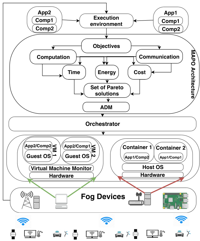
Refer to caption — Figure 1: MAPO overall architecture design.

Figure 1 describes MAPO architecture through specific case study, in which various application owners deploy their applications composed of multiple inter-connected components. The applications are deployed in the Fog through the MAPO execution environment, which acts as an interface to the MAPO architecture. Afterwards, it identifies the inter-connections among the application components following the transition function, and provides the placement constraints to the multi-objective optimization algorithm that searches for a Pareto set of tradeoff solutions considering the objectives described in Section III. The multi-objective optimization follows a relatively fast evolutionary Non-Dominated Sorting Genetic Algorithm (NSGA-II) [9] that searches for a set of non-dominated Pareto placements of the application components on a set of Fog devices. For this, it ranks the population according to a fast non-dominated sorting method to prepare elitism and good convergence near the true Pareto optimal set. An automated decision making module selects an appropriate placement based on a low latency strategy, which extends on a simple and computationally efficient a-priori method [17] assuming that all solutions on the Pareto frontier belong to a single cluster. Finally, MAPO delivers the selected placement to an orchestrator built on top of Docker Swarm [15] that operates as an execution controller that instantiates the containerized application components on the selected devices as defined in Section III-C.

V Application case studies

Table I: Application resource requirements.

Application	CPU	MEM	Storage
Application	[MI]	$\text{\,}\mathrm{\delimiter 67482370}\mathrm{\mathchar 29005}\mathrm{\mathchar 28994}\mathrm{\delimiter 84267779}$	$\text{\,}\mathrm{\delimiter 67482370}\mathrm{\mathchar 29005}\mathrm{\mathchar 28994}\mathrm{\delimiter 84267779}$
Augmented	100–	10–	256–
reality	2000	30	512
Insulin	200 –	10 –	256 –
pump	2000	60	1024
Mental	200 –	10 –	256 –
health care	2000	50	512

We selected three application case studies from the field of next generation medical applications with different computing and storage demands, summarized in Table I. We modeled every application as a state machine and labelled its transitions with the data items transferred between components, as presented in Section III-A.

Augmented reality

The medical augmented reality application broadens the surgeon’s perception of a surgical scene by merging the isolated information of the live endoscope [3]. The utilization of the Fog can significantly reduce the processing and communication latency, helping the medical professionals in close to real time scenarios. The application, divided in multiple components shown in Figure 2, fetches streamed endoscopic images²² 2 http://visurge.wp.itec.aau.at/ at specific rates (e.g., between 15 and 30 frames per second) and stitches them into a single large panorama view.

Figure 2: Augmented reality application.

Insulin pump

People who suffer from diabetes use a software-controlled system that must deliver the correct amount of insulin according to the current level of blood sugar. We modeled this software-based insulin pump [23] as a set of IoT micro-sensors embedded in the patient’s body that measure blood parameters proportional to the sugar level. In the Fog analytic layer, the system learns the patient state variation, computes the proper level of insulin upon abnormal state detection and sends it to the pump controller through eight components orchestrated as in Figure 3.

Figure 3: Insulin pump application.

Mental health care

This application [23] is used in a number of UK hospitals³³ 3 http://iansommerville.com/software-engineering-book/case-studies/the-mentcare-system/ for managing patient information suffering from a mental health disorder. As such patients may not always want to attend the same clinic, they must be helped and supported through prearranged appointments, and emergency services orchestrated in a Fog environment as illustrated in Figure 4.

Figure 4: IoT based mental health care application.

VI Experimental simulation

We implemented MAPO in the jMetal multi-objective optimization framework [10] and created elaborate scenarios based on a simulated Fog environment⁴⁴ 4 https://github.com/vindem/sleipnir, which extends the work in [6].

VI-A Experimental design

We investigate the benefits of MAPO for application placement compared to two state-of-the-art methods: Fog Service Placement Problem (FSPP) [22] based on linear integer programming and Edge-ward (EW) [13] that implements a hierarchical best fit algorithm. We consider that EW places the last component of every application on the ISP GW because of its higher computational resources. We evaluate MAPO considering the application completion time, energy consumption and economic cost required for executing an application, starting from the moment an IoT device or end-user provided the input data to the IoT application until another device or user collected the final output.

We designed two sets of experiments according to the characteristics of the low latency IoT applications described in [22]. The first experimental set investigates the impact to the objectives of the data size $\mathchar 28996\mathchar 29025\mathchar 29044\mathchar 29025_{\mathchar 29033}$ transferred between the application components set to $\{\mathchar 28720\mathchar 314\mathchar 28725\mathchar 24891\mathchar 28721\mathchar 24891\mathchar 28724\}\ $\text{\,}\mathrm{\mathchar 29005\mathchar 29026\mathchar 29033\mathchar 29044}$$ , with a fixed application CPU workload of $\mathchar 29001\mathchar 29006\mathchar 29011\mathchar 29012\mathchar 29010\left\delimiter 67273472\mathchar 29037_{\mathchar 29033}\right\delimiter 84054785\mathchar 12349\mathchar 28722\mathchar 28720\mathchar 28720\mathchar 28720$ MI. The second set of experiments evaluates the impact of the CPU workload $\mathchar 29001\mathchar 29006\mathchar 29011\mathchar 29012\mathchar 29010\left\delimiter 67273472\mathchar 29037_{\mathchar 29033}\right\delimiter 84054785\mathchar 12850\{\mathchar 28722\mathchar 28725\mathchar 28720\mathchar 24891\mathchar 28725\mathchar 28720\mathchar 28720\mathchar 24891\mathchar 28721\mathchar 28720\mathchar 28720\mathchar 28720\mathchar 24891\mathchar 28722\mathchar 28720\mathchar 28720\mathchar 28720\}$ MI by bounding the data size $\mathit{\mathchar 28996\mathchar 29025\mathchar 29044\mathchar 29025}_{\mathchar 29033}\mathchar 12349$\text{\,}\mathrm{\mathchar 29005\mathchar 29026\mathchar 29033\mathchar 29044}$$ . The objective results are then averaged over $\mathchar 28721\mathchar 28720\mathchar 28720\mathchar 28720$ runs for statistical significance.

VI-B Simulator setup

Table II and Table III display the computation and communication capabilities of the Fog devices divided in three hierarchical categories based on their computing and storage capabilities: ISP gateways (ISP GW), local WiFi gateways (WiFi GW) or cellular base transceiver station (BTS) and Mobile Edge (ME) devices. For the Cloud and ISP GW devices, we use a configuration equivalent to a system with Intel^® Xeon family (i.e. Xeon Platinum 8175). The WiFi GWs are based on an Intel^® Core^(TM) i7-8550U CPU equivalent configuration. The mobile edge devices are represented either as Raspberry Pi (RPi) single-board computers or mobile phones based on ARM Cortex-A75 architectures with Qualcomm^® Kryo^(TM) 385 equivalent cores. The devices are connected through Ethernet, Wireless LAN, or 4G/LTE network interfaces.

Table II: Fog infrastructure configuration.

	Cloud	Fog
Characteristic	CDC	ISP GW	WiFi GW/ Cellular BTS	ME
CPU [MIPS] $\mathchar 8705\mathchar 28721\mathchar 28720^{\mathchar 28723}$	250	65	[10,15]	[2,10]
RAM $\text{\,}\mathrm{\delimiter 67482370}\mathrm{\mathchar 28999}\mathrm{\mathchar 28994}\mathrm{\delimiter 84267779}$	32	16	[8,16]	[0.5,2]
Storage $\text{\,}\mathrm{\delimiter 67482370}\mathrm{\mathchar 28999}\mathrm{\mathchar 28994}\mathrm{\delimiter 84267779}$	512	250	128	16-64
$\mathchar 28965_{\mathchar 29034}^{\mathchar 29040}$ $\text{\,}\mathrm{\delimiter 67482370}\mathrm{\mathchar 29015}\mathrm{\delimiter 84267779}$	1650	530	[380,410]	[2.50,3.20]
$\mathchar 28995\mathchar 29008_{\mathchar 29034}$ [¢]	0.03	0.035	[0.04, 0.05]	[0.02,0.04]
$\mathchar 28995\mathchar 29011_{\mathchar 29034}$ [¢]	10E-7	15E-6	[10E-6,20E-6]	[20E-6, 30E-6]

Table III: Fog communication configuration.

	Cloud	Fog
Characteristic	CDC	ISP GW	WiFi GW/ Cellular BTS	ME
Connectivity	Wired	Wired	WiFi	WiFi	Cellular
Standard	IEEE 802.3a/v	IEEE 802.3a/b	IEEE 802.11a/c	IEEE 802.11a/c/n	4G/LTE
BW $\text{\,}\mathrm{\delimiter 67482370}\mathrm{\mathchar 29005}\mathrm{\mathchar 29026\mathchar 29033\mathchar 29044}\mathrm{\delimiter 68408078}\mathrm{\mathchar 29043}\mathrm{\delimiter 84267779}$	10000	[1000,2000]	[400,1000]	[250, 400]
$\mathchar 28965_{\mathchar 29034}^{\mathchar 29037}$ $\text{\,}\mathrm{\delimiter 67482370}\mathrm{\mathchar 29015}\mathrm{\delimiter 84267779}$	1300	410	[1.80,2.00]	[1.00,1.50]
$\mathchar 28995\mathchar 29010_{\mathchar 29034}$ [¢]	3E-6	35E-7	[3E-6,5E-6]	[3E-6, 5E-6]

⁴⁴footnotetext: system-on-a-chip

We simulated the Fog by considering a single geographically bounded cluster [16] with eleven ME devices connected to 90 cameras or biomedical sensors and 90 actuators. The Fog cluster is connected to a Cloud back-end infrastructure through a local proxy server. We assume that the end-users and the IoT devices are close to the MEs and experience a $\text{\,}\mathrm{\mathchar 29037\mathchar 29043}$ latency, while the latency between every ME and WiFi GW is $\text{\,}\mathrm{\mathchar 29037\mathchar 29043}$ . We set the latencies between the WiFi GW and ISP GW to $\text{\,}\mathrm{\mathchar 29037\mathchar 29043}$ , and between the ISP GW and CDC to $\text{\,}\mathrm{\mathchar 29037\mathchar 29043}$ , obtained using the Global Ping Statistics in WonderNetwork⁵⁵ 5 https://wondernetwork.com/pings.

VI-C Simulation results

We analyze the MAPO results based on three criteria: communication data size, component CPU workload, and multi-objective algorithm quality and scalability.

VI-C1 Data size

Table IV, Table V and Table VI demonstrate that the data size has marginal effect on the objective values for the augmented reality, insulin pump and mental health care applications.

More concretely, MAPO reduces the completion time by up to 70% compared to FSPP and EW, since they tend to place the application components on the ISP and WiFi GWs that are farther away from the IoT devices. This is not proper for deadline constrained applications such as the augmented reality, and results in higher communication latency. Unlike the related methods, MAPO searches for tradeoff placements by considering devices with low communication latency to the IoT layer and high computational speed and thus improves the total application completion time by reducing the communication latency and the components’ completion time locally close to the IoT devices. Lastly, the results show that the data size does not have significant effect on the completion time as the IoT applications exchange small data with low latency.

In terms of energy, EW consumes nearly 61% less than MAPO. Contrarily, MAPO reduces the energy consumption by 17% compared with FSPP. The only exception is the augmented reality application, for which MAPO provides more energy demanding solutions than FSPP. The energy consumption of MAPO is explained by the tradeoff between the increased computation time per application component and the reduced communication latency. Therefore, the higher computation time introduced by the Fog devices translates into higher energy consumption for time constrained applications.

Furthermore, MAPO reduces the economic cost by up to 77% compared to EW and by 45% compared to FSPP. The total cost is directly related to the cost for application computation and the cost for data communication among the executing components. The cost reductions provided by MAPO are due to the lower communication times which drastically reduce the completion times.

Table IV: Augmented reality application completion time, energy consumption, and economic cost vs. data size.

	Time[ $\text{\,}\mathrm{\mathchar 29043}$ ]			Energy[ $\text{\,}\mathrm{\mathchar 29035\mathchar 29002}$ ]			Cost[¢]
	$\mathchar 28720\mathchar 314\mathchar 28725$	$\mathchar 28721$	$\mathchar 28724$	$\mathchar 28720\mathchar 314\mathchar 28725$	$\mathchar 28721$	$\mathchar 28724$	$\mathchar 28720\mathchar 314\mathchar 28725$	$\mathchar 28721$	$\mathchar 28724$
FSPP	0.490	0.491	0.497	18.6	18.7	18.9	0.2	0.21	0.23
EW	0.489	0.490	0.50	18.4	18.5	19.3	0.21	0.21	0.2
MAPO	0.163	0.163	0.166	34.5	34.8	49	0.11	0.12	0.16

Table V: Insulin pump application completion time, energy consumption, and economic cost vs. data size.

	Time[ $\text{\,}\mathrm{\mathchar 29043}$ ]			Energy[ $\text{\,}\mathrm{\mathchar 29035\mathchar 29002}$ ]			Cost[¢]
	$\mathchar 28720\mathchar 314\mathchar 28725$	$\mathchar 28721$	$\mathchar 28724$	$\mathchar 28720\mathchar 314\mathchar 28725$	$\mathchar 28721$	$\mathchar 28724$	$\mathchar 28720\mathchar 314\mathchar 28725$	$\mathchar 28721$	$\mathchar 28724$
FSPP	1.276	1.279	1.296	58.5	58.8	61	0.3	0.3	0.4
EW	2.448	2.454	2.492	24	24	25	0.76	0.8	0.9
MAPO	0.76	0.79	0.6	50	46	64	0.4	0.4	0.2

Table VI: Mental health care application completion time, energy consumption, and economic cost vs. data size.

	Time[ $\text{\,}\mathrm{\mathchar 29043}$ ]			Energy[ $\text{\,}\mathrm{\mathchar 29035\mathchar 29002}$ ]			Cost[ $\text{\,}\cent$ ]
	$\mathchar 28720\mathchar 314\mathchar 28725$	$\mathchar 28721$	$\mathchar 28724$	$\mathchar 28720\mathchar 314\mathchar 28725$	$\mathchar 28721$	$\mathchar 28724$	$\mathchar 28720\mathchar 314\mathchar 28725$	$\mathchar 28721$	$\mathchar 28724$
FSPP	1.36	1.37	1.40	75	76	79	0.3	0.4	0.5
EW	2.95	2.96	3.1	25.1	25.2	26.3	1	1.1	1.4
MAPO	0.868	0.870	0.879	62.5	63	65	0.4	0.4	0.4

VI-C2 CPU workload

Table VII, Table VIII and Table IX demonstrate that although all methods scale similarly in relation to CPU workloads, there are substantial performance differences. We observe that MAPO reduces the completion time by up to 60% compared to both FSPP and EW, especially for applications with complex patterns and higher number of components, such as the insulin pump and the mental health care case studies. We explain the completion time improvements by the higher communication latency of the ISP and WiFi GWs extensively exploited by FSPP and EW. As observed, MAPO provides higher gains in terms of completion time for CPU workloads above 1000 MI.

Although MAPO outperforms FSPP and reduces the energy consumption by 23% for mental health care application, it provides more energy demanding solutions than FSPP, specifically for the augmented reality application. In addition, as the energy evaluations show, EW consumes nearly 55% less energy than MAPO. Whilst MAPO increases the computation time of the application components, it reduces the communication latency, therefore decreasing the completion time. In terms of the energy consumption, the higher computation time obtained by the execution through the Fog devices leads to higher energy consumption for a specific deadline constrained application.

Moreover, MAPO decreases the economic cost by up to 50% compared with EW and 50% with FSPP. MAPO performs better than EW in terms of economic cost, because it reduces the completion time, which translates into lower financial burden. However, FSPP incurs 22% lower costs than MAPO due to the use of cheaper Cloud resource compared to the more expensive Fog, especially for high CPU workloads.

Table VII: Augmented reality application completion time, energy consumption, and economic cost vs. CPU workload.

	Time[ $\text{\,}\mathrm{\mathchar 29043}$ ]				Energy[ $\text{\,}\mathrm{\mathchar 29035\mathchar 29002}$ ]				Cost[ $\text{\,}\cent$ ]
	$\mathchar 28722\mathchar 28725\mathchar 28720$	$\mathchar 28725\mathchar 28720\mathchar 28720$	$\mathchar 28721\mathchar 28720\mathchar 28720\mathchar 28720$	$\mathchar 28722\mathchar 28720\mathchar 28720\mathchar 28720$	$\mathchar 28722\mathchar 28725\mathchar 28720$	$\mathchar 28725\mathchar 28720\mathchar 28720$	$\mathchar 28721\mathchar 28720\mathchar 28720\mathchar 28720$	$\mathchar 28722\mathchar 28720\mathchar 28720\mathchar 28720$	$\mathchar 28722\mathchar 28725\mathchar 28720$	$\mathchar 28725\mathchar 28720\mathchar 28720$	$\mathchar 28721\mathchar 28720\mathchar 28720\mathchar 28720$	$\mathchar 28722\mathchar 28720\mathchar 28720\mathchar 28720$
FSPP	0.05	0.124	0.246	0.5	1.9	4.7	9.4	18.7	0.02	0.05	0.10	0.2
EW	0.05	0.123	0.245	0.5	2	4.7	9.3	18.4	0.03	0.06	0.11	0.2
MAPO	0.05	0.119	0.132	0.2	1.5	5	24	35	0.02	0.06	0.08	0.1

Table VIII: Insulin pump application completion time, energy consumption, and economic cost vs. CPU workload.

	Time[ $\text{\,}\mathrm{\mathchar 29043}$ ]				Energy[ $\text{\,}\mathrm{\mathchar 29035\mathchar 29002}$ ]				Cost[ $\text{\,}\cent$ ]
	$\mathchar 28722\mathchar 28725\mathchar 28720$	$\mathchar 28725\mathchar 28720\mathchar 28720$	$\mathchar 28721\mathchar 28720\mathchar 28720\mathchar 28720$	$\mathchar 28722\mathchar 28720\mathchar 28720\mathchar 28720$	$\mathchar 28722\mathchar 28725\mathchar 28720$	$\mathchar 28725\mathchar 28720\mathchar 28720$	$\mathchar 28721\mathchar 28720\mathchar 28720\mathchar 28720$	$\mathchar 28722\mathchar 28720\mathchar 28720\mathchar 28720$	$\mathchar 28722\mathchar 28725\mathchar 28720$	$\mathchar 28725\mathchar 28720\mathchar 28720$	$\mathchar 28721\mathchar 28720\mathchar 28720\mathchar 28720$	$\mathchar 28722\mathchar 28720\mathchar 28720\mathchar 28720$
FSPP	0.3	0.5	0.8	1.3	3	15	29	59	0.1	0.1	0.2	0.3
EW	0.4	0.6	1.2	2.5	6	6	12	24	0.04	0.2	0.4	0.8
MAPO	0.2	0.4	0.5	0.8	1	12	23	50	0.1	0.1	0.2	0.4

Table IX: Mental health care completion time, energy consumption and economic cost vs. CPU workload.

	Time[ $\text{\,}\mathrm{\mathchar 29043}$ ]				Energy[ $\text{\,}\mathrm{\mathchar 29035\mathchar 29002}$ ]				Cost[ $\text{\,}\cent$ ]
	$\mathchar 28722\mathchar 28725\mathchar 28720$	$\mathchar 28725\mathchar 28720\mathchar 28720$	$\mathchar 28721\mathchar 28720\mathchar 28720\mathchar 28720$	$\mathchar 28722\mathchar 28720\mathchar 28720\mathchar 28720$	$\mathchar 28722\mathchar 28725\mathchar 28720$	$\mathchar 28725\mathchar 28720\mathchar 28720$	$\mathchar 28721\mathchar 28720\mathchar 28720\mathchar 28720$	$\mathchar 28722\mathchar 28720\mathchar 28720\mathchar 28720$	$\mathchar 28722\mathchar 28725\mathchar 28720$	$\mathchar 28725\mathchar 28720\mathchar 28720$	$\mathchar 28721\mathchar 28720\mathchar 28720\mathchar 28720$	$\mathchar 28722\mathchar 28720\mathchar 28720\mathchar 28720$
FSPP	0.41	0.6	0.8	1.4	8	19	37	75	0.1	0.1	0.2	0.3
EW	0.31	0.8	1.5	2.9	3	6	13	25	0.2	0.3	0.5	0.9
MAPO	0.25	0.5	0.6	0.9	1	10	32	63	0.1	0.2	0.2	0.4

VI-C3 Multi-objective algorithm

As our research deals with an NP-complete multi-objective problem, we present experiments that demonstrates the ability of MAPO to provide high quality placements across a large set of Fog devices. Figure 5a presents the correlation between the number of evaluated placements, gradually increased from 1000 to 14000 with a population of 100 individuals, the quality of the solutions quantified by the hypervolume [25], and the execution time metrics. The results show that MAPO reaches the best solutions for around 12500 evaluations, and its execution time gradually increases with the number of evaluations, although it needs only $\text{\,}\mathrm{\mathchar 29037\mathchar 29043}$ for 14000 evaluations. In terms of scalability for finding placements with a hypervolume of $\mathchar 28720\mathchar 314\mathchar 28727$ , Figure 5b shows that MAPO’s execution time increases by 43% when the number of components increments from 5 to 30 while maintaining the quality of the solutions relatively constant.

(a)

(b)

Figure 5: MAPO hypervolume and execution time of Pareto-optimal placements with different: a) number of evaluations, b) number of application components.

VII Real-world evaluation

To validate the simulation results, we present in this section an analysis of MAPO on a real-world experimental testbed.

VII-A Experimental design

We evaluated MAPO using the mental health care application and compared it to the related FSPP and EW approaches.

We configured the components to generate a computational workload in the range $\mathchar 29001\mathchar 29006\mathchar 29011\mathchar 29012\mathchar 29010\left\delimiter 67273472\mathchar 29037_{\mathchar 29033}\right\delimiter 84054785\mathchar 12850\{\mathchar 28722\mathchar 28725\mathchar 28720\mathchar 24891\mathchar 28725\mathchar 28720\mathchar 28720\mathchar 24891\mathchar 28721\mathchar 28720\mathchar 28720\mathchar 28720\mathchar 24891\mathchar 28722\mathchar 28720\mathchar 28720\mathchar 28720\}$ (MI), with an input data set $\mathchar 28996\mathchar 29025\mathchar 29044\mathchar 29025_{\mathchar 29033}\mathchar 12850\{\mathchar 28720\mathchar 314\mathchar 28725\mathchar 24891\mathchar 28721\mathchar 24891\mathchar 28724\}$ ( $\text{\,}\mathrm{\mathchar 29005\mathchar 29026\mathchar 29033\mathchar 29044}$ ), according to the low latency IoT application characteristics described in [22].

Table X: Real-world testbed configuration.

	Cloud	Fog
Characteristic	CDC	GW	ME
CPU [MIPS] $\mathchar 8705\mathchar 28721\mathchar 28720^{\mathchar 28723}$	250	65	65
RAM $\text{\,}\mathrm{\delimiter 67482370}\mathrm{\mathchar 28999}\mathrm{\mathchar 28994}\mathrm{\delimiter 84267779}$	16	1	1
Storage $\text{\,}\mathrm{\delimiter 67482370}\mathrm{\mathchar 28999}\mathrm{\mathchar 28994}\mathrm{\delimiter 84267779}$	256	64	64
BW $\text{\,}\mathrm{\delimiter 67482370}\mathrm{\mathchar 29005}\mathrm{\mathchar 29026\mathchar 29033\mathchar 29044}\mathrm{\delimiter 68408078}\mathrm{\mathchar 29043}\mathrm{\delimiter 84267779}$	1000	1000	1000

VII-B Testbed setup

We design two sets of experiments. The first experimental set investigates the impact to the objectives of the data size $\mathchar 28996\mathchar 29025\mathchar 29044\mathchar 29025_{\mathchar 29033}$ transferred between the application components set to $\{\mathchar 28720\mathchar 314\mathchar 28725\mathchar 24891\mathchar 28721\mathchar 24891\mathchar 28724\}\ $\text{\,}\mathrm{\mathchar 29005\mathchar 29026\mathchar 29033\mathchar 29044}$$ , by considering a fixed application CPU workload of $\mathchar 29001\mathchar 29006\mathchar 29011\mathchar 29012\mathchar 29010\left\delimiter 67273472\mathchar 29037_{\mathchar 29033}\right\delimiter 84054785\mathchar 12349\mathchar 28722\mathchar 28720\mathchar 28720\mathchar 28720$ MI. The second set of experiments evaluates the impact of the CPU workload $\mathchar 29001\mathchar 29006\mathchar 29011\mathchar 29012\mathchar 29010\left\delimiter 67273472\mathchar 29037_{\mathchar 29033}\right\delimiter 84054785\mathchar 12850\{\mathchar 28722\mathchar 28720\mathchar 28720\mathchar 24891\mathchar 28725\mathchar 28720\mathchar 28720\mathchar 24891\mathchar 28721\mathchar 28720\mathchar 28720\mathchar 28720\mathchar 24891\mathchar 28722\mathchar 28720\mathchar 28720\mathchar 28720\}$ MI by bounding the data size $\mathit{\mathchar 28996\mathchar 29025\mathchar 29044\mathchar 29025}_{\mathchar 29033}\mathchar 12349$\text{\,}\mathrm{\mathchar 29005\mathchar 29026\mathchar 29033\mathchar 29044}$$ .

We prepared an in-lab experimental testbed consisting of four Raspberry Pi-3 B+ single-board computers (RPi), three of which act as ME and one acts as a GW. As a CDC device, we use a virtual machine running in a private Cloud with an eight-core Intel^® Core^(TM) i7-7700 CPU at $\text{\,}\mathrm{\mathchar 28999\mathchar 29000\mathchar 29050}$ and $\text{\,}\mathrm{\mathchar 28999\mathchar 28994}$ of RAM, running Ubuntu 16.04 LTS. The testbed components were interconnected with a dedicated Gigabit Ethernet switch and secured using the SSH protocol (see Table X). We assumed that the IoT devices are close to the MEs with an average latency of $\text{\,}\mathrm{\mathchar 29037\mathchar 29043}$ . The latency between ME and GW is $\text{\,}\mathrm{\mathchar 29037\mathchar 29043}$ , and between GW and CDC of $\text{\,}\mathrm{\mathchar 29037\mathchar 29043}$ , obtained using the Global Ping Statistics in WonderNetwork⁵. For emulating the latency between devices, we created artificial network delays using the Linux tc⁶⁶ 6 https://linux.die.net/man/8/tc command [11]. We used the nc command for data communication between containerized application components running on different devices.

We installed Raspbian GNU/Linux 9.8 (stretch)⁷⁷ 7 https://www.raspberrypi.org/downloads/raspbian/ and Docker version 18.09⁸⁸ 8 https://www.docker.com/ on all RPis and deployed a containerized virtualization environment [12]. We instantiate a Docker image on the CDC and the Fog devices by starting an Ubuntu:14.04 base image.

VII-C Real-world testbed results

We examine the real-world testbed results using two parameters as in the simulation experiments: communication data size, and component CPU workload. The results from this section confirm the general trends identified in the simulation testbed.

VII-C1 Data size

Figure 6 shows that the completion time and the energy consumption are marginally affected by the communication data sizes, regardless of the placement method. The only exception is FSPP, which induces up to 30% longer completion times for $\text{\,}\mathrm{\mathchar 29005\mathchar 29026\mathchar 29033\mathchar 29044}$ data size, as it optimizes a set of applications in a coarse-grained manner by giving priority to the CDC even for applications with small data sizes. On the other hand, there is an observable difference in the economic cost, which increases linearly with the data size. With respect to the evaluation objectives, MAPO reduces the completion time of the application case study by up to 6.9 times compared to EW, and by 3 times compared to FSPP, which in turn performs 2.3 times better than EW. The lower completion time is due to the tendency of MAPO to optimize not only the processing time, but also the communication latency, which in turn results in a reduction of the total application completion time. In terms of the energy consumption, MAPO provides an improvement of up to 35% compared to EW, and 68% compared to FSPP. Finally, MAPO provides placements up to 25% cheaper than EW, and 20% more expensive than FSPP, which provides the most economic placements due to the frequent Cloud utilization.

Figure 6: Mental health care application time, energy, and cost for different data sizes.

VII-C2 CPU workload

For a fixed data size of $\text{\,}\mathrm{\mathchar 29005\mathchar 29026\mathchar 29033\mathchar 29044}$ , Figure 7 shows that MAPO performs two, and three times, respectively, better than FSPP and EW for varying CPU workloads of up to 2000 MI. This is due to the multi-objective nature of MAPO, which considers the component execution locality, and the communication latency together with available resources. Furthermore, Figure 7 shows that MAPO provides up to 66% higher energy efficiency than FSPP. Nevertheless, MAPO is 54% less energy efficient than EW. For higher CPU workloads, MAPO gives preference to the energy consuming CDC device, thus achieving a tradeoff between the energy consumption and the completion time. Finally, MAPO provides a nearly equal economic cost to the Cloud-bounded FSPP, and 27%, on average, lower cost compared to EW as observed in the simulation.

Figure 7: Mental health care application time, energy, and cost for different CPU workloads.

VIII Conclusion and future work

We introduced MAPO, a multi-objective based application placement approach that considers both computation and communication aspects for executing IoT applications in a Fog infrastructure. MAPO employs a genetic multi-objective optimization algorithm considering three conflicting criteria: completion time, energy consumption and economic cost. To solve this problem, MAPO identifies the inter-connections among the application components, searches for a Pareto set of tradeoff solutions and selects an appropriate placement. We evaluated MAPO for three different medical applications on a simulated and a real-world testbed infrastructure, and provided a comparison with two related methods. Our results show that the MAPO placement is capable to reduce the application completion time 7.3 times while improving the energy efficiency, and decreasing the economic costs by up to 27%. The results also show that the Fog infrastructure is more energy efficient for small applications that do not require high computing resources. In addition, the communication latency has a larger impact on the completion time than the communicating data size itself.

In the future, we plan to extend MAPO to support fault tolerance for application deployment in a wide area Fog environment.

Acknowledgement

Austrian Research Promotion Agency (FFG), project 848448, Tiroler Cloud, funded this work.

References

[1] Mohammad Aazam and Eui-Nam Huh. Dynamic resource provisioning through fog micro datacenter. In Pervasive Computing and Communication Workshops (PerCom Workshops), International Conference on, pages 105–110. IEEE, 2015.
[2] Muhammad Alam, Joao Rufino, Joaquim Ferreira, Syed Hassan Ahmed, Nadir Shah, and Yuanfang Chen. Orchestration of microservices for iot using docker and edge computing. IEEE Communications Magazine, 56(9):118–123, 2018.
[3] Tobias Bergen and Thomas Wittenberg. Stitching and surface reconstruction from endoscopic image sequences: A review of applications and methods. IEEE J. Biomedical and Health Informatics, 20(1):304–321, 2016.
[4] Luiz F Bittencourt, Javier Diaz-Montes, Rajkumar Buyya, Omer F Rana, and Manish Parashar. Mobility-aware application scheduling in fog computing. IEEE Cloud Computing, 4(2):26–35, 2017.
[5] Flavio Bonomi, Rodolfo Milito, Jiang Zhu, and Sateesh Addepalli. Fog computing and its role in the internet of things. In Proceedings of the first edition of the MCC workshop on Mobile cloud computing, pages 13–16. ACM, 2012.
[6] A. Brogi, S. Forti, and A. Ibrahim. How to best deploy your fog applications, probably. In 1st IEEE International Conference on Fog and Edge Computing (ICFEC), pages 105–114, 2017.
[7] Jie Cao, Quan Zhang, and Weisong Shi. Challenges and opportunities in edge computing. In Edge Computing: A Primer, pages 59–70. Springer, 2018.
[8] Vincenzo De Maio and Ivona Brandic. First hop mobile offloading of dag computations. In 2018 18th IEEE/ACM International Symposium on Cluster, Cloud and Grid Computing (CCGRID), pages 83–92. IEEE, 2018.
[9] Kalyanmoy Deb, Amrit Pratap, Sameer Agarwal, and TAMT Meyarivan. A fast and elitist multiobjective genetic algorithm: Nsga-ii. IEEE transactions on evolutionary computation, 6(2):182–197, 2002.
[10] Juan J Durillo and Antonio J Nebro. jmetal: A java framework for multi-objective optimization. Advances in Engineering Software, 42(10):760–771, 2011.
[11] Ali Fahs and Guillaume Pierre. Proximity-aware traffic routing in distributed fog computing platforms. In IEEE/ACM International Symposium in Cluster, Cloud, and Grid Computing (CCGrid), 2019.
[12] Wes Felter, Alexandre Ferreira, Ram Rajamony, and Juan Rubio. An updated performance comparison of virtual machines and linux containers. In 2015 IEEE international symposium on performance analysis of systems and software (ISPASS), pages 171–172. IEEE, 2015.
[13] Harshit Gupta, Amir Vahid Dastjerdi, Soumya K Ghosh, and Rajkumar Buyya. ifogsim: A toolkit for modeling and simulation of resource management techniques in the internet of things, edge and fog computing environments. Software: Practice and Experience, 47(9):1275–1296, 2017.
[14] Majid Hajibaba and Saeid Gorgin. A review on modern distributed computing paradigms: Cloud computing, jungle computing and fog computing. Journal of computing and information technology, 22(2):69–84, 2014.
[15] Saiful Hoque, Mathias Santos de Brito, Alexander Willner, Oliver Keil, and Thomas Magedanz. Towards container orchestration in fog computing infrastructures. In 2017 IEEE 41st Annual Computer Software and Applications Conference (COMPSAC), volume 2, pages 294–299. IEEE, 2017.
[16] Dragi Kimovski, Humaira Ijaz, Nishant Saurabh, and Radu Prodan. Adaptive nature-inspired fog architecture. In Fog and Edge Computing (ICFEC), 2018 IEEE 2nd International Conference on, pages 1–8. IEEE, 2018.
[17] Dragi Kimovski, Sashko Ristov, Roland Mathá, and Radu Prodan. Multi-objective service oriented network provisioning in ultra-scale systems. In European Conference on Parallel Processing, pages 529–540. Springer, 2017.
[18] Redowan Mahmud, Kotagiri Ramamohanarao, and Rajkumar Buyya. Latency-aware application module management for fog computing environments. ACM Transactions on Internet Technology (TOIT), 2018.
[19] Matteo Nardelli, Stefan Nastic, Schahram Dustdar, Massimo Villari, and Rajiv Ranjan. Osmotic flow: Osmotic computing+ iot workflow. IEEE Cloud Computing, 4(2):68–75, 2017.
[20] Claus Pahl, Antonio Brogi, Jacopo Soldani, and Pooyan Jamshidi. Cloud container technologies: a state-of-the-art review. IEEE Transactions on Cloud Computing, 2017.
[21] Xuan-Qui Pham and Eui-Nam Huh. Towards task scheduling in a cloud-fog computing system. In Network Operations and Management Symposium (APNOMS), 2016 18th Asia-Pacific, pages 1–4. IEEE, 2016.
[22] Olena Skarlat, Matteo Nardelli, Stefan Schulte, and Schahram Dustdar. Towards qos-aware fog service placement. In Fog and Edge Computing (ICFEC), 2017 IEEE 1st International Conference on, pages 89–96. IEEE, 2017.
[23] Ian Sommerville. Software engineering 9th edition. ISBN-10, 137035152, 2011.
[24] Yan Sun, Fuhong Lin, and Haitao Xu. Multi-objective optimization of resource scheduling in fog computing using an improved nsga-ii. Wireless Personal Communications, pages 1–17, 2018.
[25] Lyndon While, Philip Hingston, Luigi Barone, and Simon Huband. A faster algorithm for calculating hypervolume. IEEE transactions on evolutionary computation, 10(1):29–38, 2006.
[26] Ye Xia, Xavier Etchevers, Loic Letondeur, Adrien Lebre, Thierry Coupaye, and Frédéric Desprez. Combining heuristics to optimize and scale the placement of iot applications in the fog. In 11th IEEE/ACM Conference on Utility and Cloud Computing, UCC 2018, 2018.