Spectral theory of imperfect diffusion-controlled reactions
on heterogeneous catalytic surfaces
Abstract
We propose a general theoretical description of chemical reactions occurring on a catalytic surface with heterogeneous reactivity. The propagator of a diffusion-reaction process with eventual absorption on the heterogeneous partially reactive surface is expressed in terms of a much simpler propagator toward a homogeneous perfectly reactive surface. In other words, the original problem with general Robin boundary condition that includes in particular mixed Robin-Neumann condition, is reduced to that with Dirichlet boundary condition. Chemical kinetics on the surface is incorporated as a matrix representation of the surface reactivity in the eigenbasis of the Dirichlet-to-Neumann operator. New spectral representations of important characteristics of diffusion-controlled reactions, such as the survival probability, the distribution of reaction times, and the reaction rate, are deduced. Theoretical and numerical advantages of this spectral approach are illustrated by solving interior and exterior problems for a spherical surface that may describe either an escape from a ball or hitting its surface from outside. The effect of continuously varying or piecewise constant surface reactivity (describing, e.g., many reactive patches) is analyzed.
Keywords:
Propagator; Mixed boundary condition; Partial reactivity; Heterogeneity; Reaction rate; Dirichlet-to-Neumann operatorpacs
02.50.-r, 05.60.-k, 05.10.-a, 02.70.RrI Introduction
Marian von Smoluchowski first emphasized the importance of diffusive dynamics of reactant molecules and thus laid the foundations for the modern theory of diffusion-controlled reactions Smoluchowski17. In the basic description, the concentration of molecules, diffusing toward a static catalytic surface with the diffusivity , obeys the diffusion equation in a bulk domain
| (1) |
(with being the Laplace operator), subject to the Dirichlet boundary condition on the surface :
| (2) |
This condition describes a perfect sink, i.e., any molecule hitting the surface reacts with infinite reaction rate upon the first encounter. Since that seminal paper by Smoluchowski, diffusion-controlled reactions to perfect sinks and the related first-passage phenomena have been thoroughly investigated Rice85; Redner; Levitz06; Condamin07; Benichou10b; Benichou14; Metzler.
The assumption of infinite reaction rate is not realistic for most chemical reactions because a molecule that approached a catalytic surface, needs to overcome an activation energy barrier to react that results in a finite reaction rate Weiss86; Hanggi90. This effect was first incorporated by Collins and Kimball Collins49 who replaced Dirichlet boundary condition (2) by Robin boundary condition (also known as Fourier, radiation, or third boundary condition):
| (3) |
where is the normal derivative oriented outward the bulk. This condition states that at each boundary point , the diffusive flux density, , in the unit direction orthogonal to the surface, is proportional to the concentration at this point. The proportionality coefficient, , is called the reactivity (with units m/s) and can in general depend on the point . In this formulation, Robin boundary condition is essentially a mass conservation law at each point of the boundary: the net influx of molecules diffusing toward the boundary is equal to the amount of reacted molecules. The limit (for all ) describes an inert surface without any reaction (i.e., the net diffusive flux at the surface is zero), whereas the limit reduces Eq. (3) to Eq. (2) and describes an immediate reaction upon the first encounter. The reactivity is thus related to the probability of reaction event at the encounter Filoche99; Grebenkov03; Grebenkov06a. Robin boundary condition with homogeneous (constant) reactivity was often employed to describe many chemical and biochemical reactions and permeation processes Lauffenburger; Sano79; Sano81; Shoup82; Sapoval94; Sapoval02; Grebenkov05; Qian06; Traytak07; Bressloff08; Galanti16; Grebenkov19b, to model stochastic gating Benichou00; Reingruber09; Lawley15; Bressloff17, or to approximate the effect of microscopic heterogeneities in a random distribution of reactive sites Berg77; Shoup81; Zwanzig91 (see a recent overview in Grebenkov19).
In spite of its practical importance, diffusion-controlled reactions with heterogeneous surface reactivity remain much less studied. In fact, when is not constant, the eigenfunctions of the Laplace operator with Robin boundary condition are not known explicitly even for simple domains (e.g. a ball) that prohibits using standard spectral decompositions Carslaw; Crank, on which most of classical solutions are based. One needs therefore to resort to numerical tools such as finite element or finite difference methods for solving the diffusion equation, or to Monte Carlo simulations. A notable exception is the case of piecewise constant reactivity that describes a target (or multiple targets ) with a constant reactivity on the otherwise inert surface. This situation corresponds to Robin-Neumann (for ) or Dirichlet-Neumann (for ) mixed boundary conditions Sneddon; Duffy. The Dirichlet-Neumann boundary value problem has been particularly well studied for the Poisson and Laplace equations determining the mean first-passage time to a small target and the reaction rate, respectively (see overviews in Holcman14; Schuss; Holcman and references therein). On one hand, matched asymptotic analysis, dual series technique, and conformal mapping were applied to establish the behavior of the mean first-passage time in both two- and three-dimensional domains Singer06a; Singer06b; Singer06c; Pillay10; Cheviakov10; Cheviakov12; Caginalp12; Marshall16; Grebenkov16c. On the other hand, homogenization techniques were used to substitute piecewise constant reactivity by an effective homogeneous reactivity Berg77; Shoup81; Zwanzig90; Zwanzig91; Berezhkovskii04; Berezhkovskii06; Muratov08; Bernoff18b; Dagdug16; Lindsay17; Bernoff18a. More recent works investigated how the mean reaction time is affected by a finite lifetime of diffusing particles Yuste13; Meerson15; Grebenkov17d, by partial reactivity and interactions Grebenkov17a; Agranov18, by target aspect ratio Grebenkov17b, by reversible target-binding kinetics Grebenkov17c; Lawley19 and surface-mediated diffusion Benichou10; Benichou11; Rupprecht12a; Rupprecht12b, by heterogeneous diffusivity Vaccario15, and by rapid re-arrangments of the medium Jain16; Lanoiselee18; Sposini19. Some of the related effects onto the whole distribution of reaction times were analyzed Godec16a; Godec16b; Grebenkov18; Grebenkov18c; Hartich18. However, the current understanding of diffusion-controlled reactions on catalytic surfaces with continuously varying heterogeneous reactivity remains episodic.
In this paper, we propose a mathematical description of diffusion-controlled reactions on catalytic surfaces, in which chemical kinetics, characterized by heterogeneous surface reactivity , is disentangled from the first-passage diffusive steps. In Sec. II, we express the propagator of the sophisticated diffusion-reaction process with multiple reflections on partially reactive surface in terms of a much simpler Dirichlet propagator toward a homogeneous perfectly reactive surface with Dirichlet boundary condition. Chemical kinetics is incorporated via a matrix representation of the heterogeneous surface reactivity in the eigenbasis of the Dirichlet-to-Neumann operator, which is also tightly related to the Dirichlet propagator. From the propagator, we deduce other important characteristics of diffusion-controlled reactions such as the survival probability, the distribution of reaction times and the reaction rate. This formalism provides a general description of such processes and brings conceptually new tools for its investigation. In Sec. III, this spectral approach is applied to an important example of a spherical surface for which the Dirichlet propagator and the Dirichlet-to-Neumann operator are known explicitly. We study both the interior and exterior problems that may describe either an escape from a ball or hitting its surface from outside. Semi-analytical solutions for the probability density of reaction times and for the reaction rate are derived. In Sec. IV, we discuss the advantages and limitations of the spectral approach, its possible extensions, and further applications, in particular, for analytical and numerical studies of mixed boundary value problems. Technical derivations are reported in Appendices.
II General spectral description
We consider a molecule diffusing with the diffusion coefficient in an Euclidean domain toward a partially reactive catalytic boundary characterized by a prescribed heterogeneous (space-dependent) reactivity . Once the molecule hits the boundary at some point , it may either react or be reflected back to resume its diffusion until the next encounter, and so on. The reaction probability at each encounter is characterized by the reactivity at the encounter point. In this way, the molecule performs multiple diffusive excursions in the bulk until reaction occurs. The finite reactivity results therefore in a very sophisticated diffusive dynamics near the catalytic surface, which is much more intricate than just the first arrival to a homogeneous perfectly reactive surface. A probabilistic construction of this diffusive process (called partially reflected Brownian motion) was discussed in Grebenkov03; Grebenkov06a; Papanicolaou90; Bass08; Grebenkov07a; Singer08; Grebenkov09 (see an overview in Grebenkov19).
Without dwelling on the probabilistic aspects of the problem, we aim at characterizing such diffusion-reaction processes via the propagator (also known as heat kernel or Green’s function). This is the probability density for a molecule that has not reacted until time on the partially reactive boundary , to be in a vicinity of a point at time , given that it was started at a point at time . For any fixed starting point , the propagator satisfies the following boundary value problem
| (4a) | |||||
| (4b) | |||||
| (4c) | |||||
where is the Dirac distribution, and the Laplace operator acts on . If the domain is unbounded, these equations are completed by the regularity condition at infinity: as . To avoid technicalities, we assume that the boundary is smooth. The following discussion extends our former results Grebenkov06a; Grebenkov06; Grebenkov07a; Grebenkov19 to heterogeneous reactivity and time-dependent diffusion equation.
We consider the Laplace-transformed propagator,
| (5) |
which satisfies the modified Helmholtz equation for each fixed :
| (6a) | |||||
| (6b) | |||||
(tilde will denote Laplace-transformed quantities).
Our goal is to express the propagator describing diffusion toward heterogeneous partially reactive surface in terms of the much simpler Dirichlet propagator that characterizes diffusion toward the homogeneous perfectly reactive surface and satisfies for each fixed :
| (7a) | |||||
| (7b) | |||||
Due to the linearity of the problem (6), one can search its solution in the form
| (8) |
where the unknown regular part satisfies
| (9a) | |||||
| (9b) | |||||
for , where
| (10) |
is the Laplace transform of the diffusive flux density at time in a point of the homogeneous perfectly reactive surface (i.e., the probability density of the first arrival in a vicinity of at time after starting from at time ).
II.1 Dirichlet-to-Neumann operator
The solution of the boundary value problem (9) can be obtained with the help of the Dirichlet-to-Neumann operator (also known as Poincaré-Steklov operator) Egorov; Jacob; Taylor. This is a pseudo-differential self-adjoint operator that associates to a function on the boundary another function on that boundary:
| (11) |
where is the solution of the Dirichlet boundary value problem:
| (12a) | |||||
| (12b) | |||||
(here we skip the usual regularity assumptions on , as well as the explicit description of the functional spaces involved in the rigorous definition of , see Egorov; Jacob; Taylor; Marletta04; Arendt07; Arendt15; Hassell17 for details). For instance, if is understood as a source of molecules on the boundary emitted into the reactive bulk, then the operator gives their flux density on that boundary. Note that there is a family of operators parameterized by (or ).
As the solution of the Dirichlet boundary value problem (12) can be expressed in terms of the Dirichlet propagator in a standard way,
the Dirichlet-to-Neumann propagator acts formally as
| (13) |
and thus the Dirichlet propagator determines the Dirichlet-to-Neumann operator . In Appendix A, it is also shown how the Dirichlet propagator can be constructed from the operator . As a consequence, these two important objects are equivalent. As discussed in Grebenkov06a for the case , the Dirichlet-to-Neumann operator can also be interpreted as the continuous limit of the Brownian self-transport operator which was introduced in Filoche99; Grebenkov03 to describe the probability of the first arrival to a site of a discretized boundary from another site via bulk diffusion.
Let us now return to the boundary value problem (9). Suppose that we have solved this problem and found that the solution on the boundary is equal to some function . Applying then the Dirichlet-to-Neumann operator to , one can express the normal derivative of , from which
| (14) |
where is the operator of multiplication by . Knowing the restriction of on the boundary , one can reconstruct this function in the bulk as the solution of the corresponding Dirichlet problem:
| (15) |
In this way, we obtain the desired representation of the propagator in the form of a scalar product between two functions on the boundary
| (16) | |||
where denotes the standard scalar product between functions and on the boundary :
and asterisk denotes the complex conjugate. Equation (16) is the first main result of the paper. Remarkably, all the “ingredients” of this formula correspond to the Dirichlet condition on a homogeneous perfectly reactive boundary, except for the operator that keeps track of heterogeneous surface reactivity . We outline that Eq. (16) does not solve the original problem but reduces it to a much simpler and more thoroughly studied Dirichlet problem.
When and are boundary points, the identity reduces Eq. (16) to
| (17) |
i.e., is the kernel of the operator . One can therefore rewrite Eq. (16) as
| (18) | |||||
while its inverse Laplace transform reads
| (19) |
This relation expresses the propagator in the whole domain in terms of the propagator from one boundary point to another boundary point via bulk diffusion. The first term represents the contribution of direct trajectories from to that do not touch the boundary . The second term also has a simple probabilistic interpretation: a molecule reaches the boundary for the first time at , performs partially reflected Brownian motion over time (with eventual failed attempts of reaction at each encounter with the surface), and diffuses to the bulk point during time without hitting the reactive surface.
When is a boundary point, one has and , so that the integrals over and are removed, reducing Eq. (19) to
| (20) |
This relation justifies the qualitative separation of the diffusion-reaction process into two steps: the first arrival step (described by ) and the reaction step (described by ). We stress, however, that the reaction step involves intricate diffusion process near the partially reactive catalytic surface. In addition to the new conceptual view onto partially reflected Brownian motion, the representations (19, 20) can be helpful for a numerical computation of the propagator because only the boundary-to-boundary transport via needs to be determined. This kernel significantly extends the Brownian self-transport operator introduced in Filoche99; Grebenkov03 (see below).
II.2 Other common diffusion characteristics
The propagator determines many quantities often considered in the context of diffusion-controlled reactions such as the survival probability up to time , the reaction time distribution, the distribution of reaction points (at which reaction occurs), and the reaction rate. For instance, the diffusive flux density at a partially reactive point is
| (21) |
where we used the Robin boundary condition (4c). This is the joint probability density for the reaction time and the reaction point on the catalytic surface. The integral over yields the marginal probability density of reaction times,
| (22) |
whereas the integral over gives the marginal probability density of reaction points:
| (23) |
The latter was called the spread harmonic measure density Grebenkov06a; Grebenkov06; Grebenkov06b; Grebenkov15. This is a natural extension of the harmonic measure density that characterizes the first arrival onto the perfectly reactive surface Garnett; Grebenkov05a; Grebenkov05b. As the probability density can be interpreted as the probability flux onto the surface for a molecule started from , its integral with the initial concentration of molecules, , yields the overall diffusive flux onto the surface, i.e., the reaction rate:
| (24) |
In turn, the integral of from to infinity gives the survival probability up to time :
| (25) |
while is the probability of reaction up to time . All these quantities are expressed in terms of the propagator and thus determined from Eq. (16).
II.3 Spectral decompositions
When the boundary is bounded, the Dirichlet-to-Neumann operator has a discrete spectrum, with a set of nonnegative eigenvalues and -normalized eigenfunctions forming a complete orthogonal basis in :
| (26) |
We emphasize that both and depend in general on as a parameter. Expanding the scalar product in Eq. (16) over this basis, one gets
| (27) | |||
where
| (28) |
is the projection of the Laplace-transformed flux density onto the eigenfunction , and
| (29a) | |||||
| (29b) | |||||
are infinite-dimensional matrices that represent the Dirichlet-to-Neumann operator and the reactivity multiplication operator in the basis of eigenfunctions .
From the spectral representation (27) and Eq. (21), we deduce
| (30) |
where we used the completeness of eigenfunctions to represent as multiplication by the matrix . According to Eqs. (22, 23), the spectral decomposition (30) yields immediately
| (31) |
and
| (32) |
where
| (33) |
are dimensionless coefficients. In particular, is the reaction probability (in Appendix B.1, we prove the expected identity for any bounded domain). According to Eq. (24), the Laplace-transformed reaction rate is then
| (34) |
In Appendix B.2, we show how this expression can be further simplified in the case of the uniform initial concentration.
While we mainly focus on Laplace-transformed quantities, their representations in time domain can be obtained via Laplace transform inversion either analytically or numerically. For instance, the inversion in the case of bounded domains can be performed via the residue theorem by computing the poles of functions in Eqs. (27, 32, 34), which are determined by the condition
| (35) |
In general, the spectral representation (27) is not simpler than Eq. (16) because all , and depend on as a parameter. However, in some domains, these “ingredients” can be evaluated explicitly, providing a semi-analytical form of the Laplace-transformed propagator and related quantities. We will illustrate this point in Sec. III for a spherical boundary.
II.4 Homogeneous partial reactivity
In the particular case of homogeneous reactivity, , the operator is proportional to the identity operator, and Eq. (17) implies that is the resolvent of the Dirichlet-to-Neumann operator . Moreover, as
| (36) |
Eq. (27) is reduced to
| (37) |
In turn, the condition (35) on the poles is reduced to a set of decoupled equations
| (38) |
showing how the eigenvalues of the Dirichlet-to-Neumann operator determine the eigenvalues of the associated Laplace operator with Robin boundary condition.
The other spectral decompositions are also simplified:
| (39) |
| (40) |
and
| (41) |
where we used Eq. (75) for the uniform initial concentration . In the limit , one recovers the formula for the total steady-state flux derived in Ref. Grebenkov06; Eq. (41) is therefore its extension to time-dependent diffusion. To our knowledge, Eqs. (37, 39, 40, 41) that are fully explicit in terms of the eigenvalues and eigenfunctions of the Dirichlet-to-Neumann operator, have not been earlier reported. While alternative spectral decompositions on the Laplace operator eigenfunctions are known for bounded domains, there is no such expansion for unbounded domains, for which the spectrum of the Laplace operator is continuous. The spectral formulation in terms of the eigenfunctions of the Dirichlet-to-Neumann operator opens therefore new perspectives for studying diffusion-reaction processes even for homogeneous reactivity. From the numerical point of view, the computation of the eigenfunctions of the Dirichlet-to-Neumann operator could in general be simpler due to the reduced dimensionality: need to be found on the boundary , whereas the Laplace operator eigenfunctions have to be computed in the whole domain .
III Spherical boundary
In this section, we apply our general spectral decompositions to the case of a spherical boundary for which the eigenbasis of the Dirichlet-to-Neumann operator is known explicitly. We first discuss in Sec. III.1 the interior problem that may describe, for instance, an escape from a ball, and then in Sec. III.2 we dwell on the exterior problem and related chemical kinetics. In both cases, we provide semi-analytical solutions for an arbitrary heterogeneous surface reactivity and then discuss some particular cases, e.g., a piecewise constant reactivity that describes single or multiple reactive targets on the otherwise inert boundary. Technical details of calculations are reported in Appendices C, D, and E.
III.1 Diffusion inside a ball
We consider a diffusion-reaction process inside a ball of radius , , with a prescribed heterogeneous surface reactivity . For this domain, the eigenvalues and eigenfunctions of the Dirichlet-to-Neumann operator are known explicitly (Appendix C),
| (42a) | |||||
| (42b) | |||||
where are the modified spherical Bessel functions of the first kind, are the -normalized spherical harmonics, prime denotes the derivative with respect to the argument, and we used spherical coordinates . Here we employ the double index to enumerate the eigenfunctions as well as the elements of the matrices and . Note that the eigenvalues do not depend on the index and thus are of multiplicity , whereas the eigenfunctions do not depend on the parameter . The eigenvalues determine the matrix via Eq. (29a), while Eq. (29b) for the matrix reads
| (43) |
The calculation of the matrix in Eq. (43) involves integrals with spherical harmonics that can often be evaluated explicitly. In Appendix D, we discuss several common situations such as a single target, multiple non-overlapping targets of circular shape or multiple latitudinal stripes, axisymmetric reactivity , and an expansion of into a finite sum over spherical harmonics. Although cumbersome, resulting expressions for the matrix are exact and do not involve numerical quadrature, providing a powerful computational tool. These cases can further be extended by adding another concentric surface with reflecting or absorbing boundary condition. This modification does not change the matrix but affects the eigenvalues of the Dirichlet-to-Neumann operator and thus the matrix .
As the Dirichlet propagator is also known, we deduce in Appendix C
| (44) |
so that the Laplace-transformed propagator is determined in the semi-analytical form (27), in which the dependence on points and is fully explicit, whereas the computation of the coefficients involves a numerical inversion of the matrix . Similarly, one gets semi-analytical expressions for the Laplace-transformed probability density of reaction times and the spread harmonic measure (see Appendix C), e.g.,
| (45) |
with
| (46) |
The Laplace-transformed survival probability is related to as
| (47) |
whereas the mean reaction time is simply .
Figures 1(b,c) illustrate how the mean reaction time depends on the starting point for a particular choice of a continuously varying heterogeneous surface reactivity shown in Fig. 1(a). When the mean reactivity is weak (, Fig. 1(b)), is close to the mean reaction time corresponding to homogeneous reactivity . Here, multiple failed reaction attempts homogenize the mean reaction time, even though the starting point lies on the catalytic boundary. In turn, significant deviations from are observed at a larger mean reactivity . In this case, the mean reactivity is not representative and heterogeneities start to be more and more important.


III.2 Diffusion outside a ball
For diffusion in the unbounded domain outside the spherical surface of radius , the eigenfunctions of the Dirichlet-to-Neumann operator are still given by Eq. (42b), so that the matrix remains unchanged. In turn, the matrix is now determined by the eigenvalues
| (48) |
where are the modified spherical Bessel function of the second kind. From the known Dirichlet propagator, we compute in Appendix E
| (49) |
As a consequence, our spectral decomposition (27) fully determines the Laplace-transformed propagator . The Laplace-transformed probability density of reaction times is again obtained from Eq. (32):
| (50) |
with given by Eq. (46), in which the matrices and are determined by Eqs. (43, 48). The Laplace-transformed survival probability is still given by Eq. (47), while the mean reaction time is infinite.
According to Eq. (34), the Laplace-transformed reaction rate can be obtained by integrating with the initial concentration of molecules, which for the uniform concentration, , yields
| (51) |
(note that the same formula with the appropriate matrix holds for diffusion inside the ball). The prefactor is the Smoluchowski rate to a homogeneous perfectly reactive ball of radius , whereas the second factor describes the effect of heterogeneous surface reactivity. In the limit , this expression yields the steady-state reaction rate
| (52) |
For the homogeneous reactivity, our formulas are reduced to that of Collins and Kimball Collins49, see Appendix E, with
| (53) |
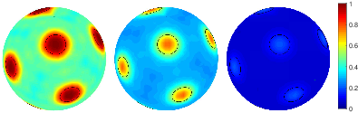
Figure 2 shows the reaction probability from Eq. (50) (see also Eq. (127)) on the inert spherical surface covered by ten evenly distributed circular partially reactive targets of angular size . Even though the starting point lies on the surface (), the reaction probability is not equal to due to the partial reactivity and eventual failed attempts to react. When the reactivity is large (, left panel), the reaction probability is close to when the molecule starts at any target, and drops to in between two targets. At intermediate reactivity (, middle panel), the reaction probability is expectedly reduced, as more frequent failed reaction attempts give more chances for the molecule to escape to infinity. This effect is further enhanced at even smaller reactivity (right panel). In this regime, there is almost no distinction between weakly reactive targets and the remaining inert surface.
IV Discussion
We developed a general mathematical description of diffusion-controlled reactions on catalytic surfaces with heterogeneous reactivity . We showed how the propagator of the diffusion equation with Robin boundary condition can be expressed in terms of the Dirichlet propagator for homogeneous perfectly reactive surface. The latter involves much simpler and more studied Dirichlet boundary condition and thus describes exclusively the first-passage events to the boundary that are independent of the surface reactivity. In other words, the diffusive exploration of the bulk is disentangled from the chemical kinetics on the boundary. As a consequence, the Dirichlet propagator needs to be computed only once for a given geometric configuration, offering a powerful theoretical and numerical tool for investigating the effects of heterogeneous surface reactivity.
Numerical or eventually analytical inversion of the Laplace transform allows one to recover the propagator in time domain. Moreover, the Laplace-transformed propagator itself is important as it describes the steady-state diffusion of molecules which may spontaneously disappear in the bulk with the rate Yuste13; Meerson15; Grebenkov17d. Such “mortal walkers” may represent radioactive nuclei, photobleaching fluorophores, molecules in an excited state, metastable complexes, spermatozoa, and other particles subject to spontaneous decay, disintegration, ground state recovery, or death.
When the boundary of the domain is bounded, our general representation yields the spectral decompositions of the propagator and of other important quantities such as the survival probability, the probability density of reaction times, the spread harmonic measure, and the reaction rate. These decompositions involve the eigenvalues and eigenfunctions of the Dirichlet-to-Neumann operator, as well as the associated basis elements of the surface reactivity . This spectral description brings new insights onto imperfect diffusion-controlled reactions and creates a mathematical basis for formulating and solving optimization and inverse problems on surface reactivity (see, e.g., Nguyen10; Filoche08).
We highlight a similarity between the representation of surface reactivity in the eigenbasis of the Dirichlet-to-Neumann operator and the representation of the bulk reactivity in the Laplace operator eigenbasis studied in Nguyen10. Such matrix representations have proved to be efficient for solving numerically the Bloch-Torrey equation that describes diffusion magnetic resonance imaging (see Grebenkov07; Grebenkov08; Grebenkov16d and references therein). Note that the surface reactivity could also be incorporated via the Laplacian eigenbasis by introducing an infinitely thin reactive boundary layer as discussed in Grebenkov07a; Grebenkov09. However, the eigenbasis of the Dirichlet-to-Neumann operator acting on the boundary seems to be more natural for dealing with surface reactivity. Most importantly, our spectral description is also valid for exterior problems, for which the spectrum of the Laplace operator is continuous and thus not suitable for such representations; in turn, the spectrum of the Dirichlet-to-Neumann operator on a bounded boundary remains discrete.
We applied the spectral approach to an important example of a spherical surface, for which both the Dirichlet propagator and the eigenbasis of the Dirichlet-to-Neumann operator are known explicitly. In this case, the Robin propagator and the related quantities (such as the probability density of reaction times) are obtained in a semi-analytical form, in which the dependence on the starting and arrival points is fully explicit, whereas the coefficients need to be computed by truncating and inverting an explicitly known matrix. However, the proposed approach is not limited to the spherical boundary. For instance, the case of a hyperplane was partly studied in Sapoval05; Grebenkov19; apart from straightforward extensions to disks and cylinders, one can consider more complicated catalytic surfaces formed by multiple non-overlapping spheres, for which the Dirichlet propagator in the steady-state regime was recently investigated in Grebenkov19b. In general, the eigenbasis of the Dirichlet-to-Neumann operator can be constructed numerically; since is independent of the surface reactivity, this construction has to be performed only once for a given catalytic surface.
As mentioned earlier, most former studies focused on the mixed Dirichlet-Neumann boundary value problem describing perfectly reactive targets on an otherwise inert boundary. In spite of its oversimplified character from the chemical point of view, this problem may look simpler from the mathematical point of view. For instance, as both Dirichlet and Neumann boundary conditions are conformally invariant, conformal mapping results in a universal integral representation of the mean first-passage time for planar domains Grebenkov16c. In addition, the technique of dual series is more developed for this case Sneddon; Duffy. At the same time, mixed Dirichlet-Neumann condition is the most problematic from the perspective of the present work. Even though the Dirichlet boundary condition can be formally implemented by setting on the target and then letting go to infinity, an infinitely large jump of reactivity at the border of the target requires elaborate asymptotic analysis. In fact, this limit is in general highly nontrivial because the unbounded Dirichlet-to-Neumann operator cannot be neglected as compared to the bounded operator (representing the reactivity) even as . This situation resembles the asymptotic analysis of the Schrödinger operator in the semi-classical limit , where is a bounded potential. While the application of asymptotic techniques from spectral theory and quantum mechanics to our setting presents an interesting mathematical perspective for future research, our spectral approach is not well suited for studying mixed Dirichlet-Neumann boundary value problems.
Similarly, in the narrow escape limit (when targets are very small), a large number of eigenfunctions of the Dirichlet-to-Neumann operator is needed to accurately represent the multiplication operator by a truncated matrix , making numerical computations time-consuming. More generally, when the shape of the boundary is rather complex or not smooth enough (e.g., containing corners or cusps), the computation of the Dirichlet-to-Neumann eigenfunctions becomes difficult, whereas a large number of eigenfunctions may be needed to project even a smooth surface reactivity. In other words, when the surface reactivity has a substantial projection on a large number of eigenfunctions, the “effective” dimensionality of the matrix can be large, making the proposed spectral approach less efficient from the numerical point of view. Nevertheless, the present approach can still be advantageous for exterior problems, which are particularly difficult to deal with by other numerical techniques. In this light, the present approach does not substitute conventional techniques but aims to complement them by addressing imperfect diffusion-controlled reactions on catalytic surfaces with finite continuously varying heterogeneous reactivity.
Appendix A Alternative representation based on the fundamental solution
In this Appendix, we describe an alternative scheme for representing the propagator in terms of the fundamental solution of the modified Helmholtz equation.
A.1 Dirichlet propagator and the Dirichlet-to-Neumann operator
The Laplace-transformed Dirichlet propagator and the Dirichlet-to-Neumann operator are closely related. On one hand, the action of onto a given function can be expressed via Eq. (13) in terms of the propagator by solving the corresponding Dirichlet boundary value problem. On the other hand, the Dirichlet propagator can be constructed explicitly from the Dirichlet-to-Neumann operator. For this purpose, one can first represent the propagator as
| (54) |
where
| (55) |
is the fundamental solution of the modified Helmholtz equation in three dimensions,
| (56) |
whereas is the regular part of the propagator satisfying, for any fixed ,
| (57a) | |||||
| (57b) | |||||
Here we use hat instead of tilde in order to distinguish the involved quantities from those in Sec. II.3.
The above problem can be solved in a standard way by using the Dirichlet propagator :
Using the boundary condition (57b) and substituting the representation (54), one gets
| (58) | |||||
where
| (59) |
is also a fully explicit function, and we used the Dirichlet-to-Neumann operator , acting on as a function of a boundary point , to represent the normal derivative of . Combining Eqs. (54, 58), we get the representation of the Dirichlet propagator in terms of the Dirichlet-to-Neumann operator and fully explicit functions and .
A.2 General Robin boundary value problem
Similarly, for a given function on the boundary , the solution of a general Robin boundary value problem
| (60a) | |||||
| (60b) | |||||
can be obtained by multiplying Eqs. (56, 60a) by and respectively, subtracting them, integrating over , and applying the Green’s formula:
| (61) | |||||
This is a standard representation of a solution of the modified Helmholtz equation in terms of the surface integral with the potential and its normal derivative . Here, in a bulk point is determined by its values and its normal derivative on the boundary. In turn, the Robin boundary condition (60b) can be expressed in terms of the Dirichlet-to-Neumann operator and the operator of multiplication by as , from which Eq. (61) yields
| (62) |
Since the operator is self-adjoint, this solution can also be written as
| (63) |
If the boundary is bounded, the spectrum of is discrete, and this solution can be written as a spectral decomposition:
| (64) | |||||
where
| (65) |
and the matrices and are defined in Eq. (29a). In particular, the Laplace-transformed propagator for the Robin boundary value problem (6) can be written as
| (66) |
where
| (67) |
In contrast to Eq. (27), this representation is based on the explicitly known fundamental solution and does not involve the Dirichlet propagator . As a consequence, all the deduced spectral decompositions rely uniquely on the eigenbasis of the Dirichlet-to-Neumann operator. While the representations (27) and (66) are equivalent and complementary to each other, we keep using the former one due to its simpler form and clearer probabilistic interpretation.
Appendix B Technical derivations
B.1 Reaction probability
The reaction probability can be obtained by integrating the probability density of reaction times over from to infinity, giving . For any bounded domain, a diffusing molecule cannot avoid the reaction event so that , ensuring the correct normalization of the probability density . This property can be checked directly from our spectral representation (32). Setting yields the reaction probability
| (68) | |||||
For any bounded domain, the Laplace equation with on the boundary has the constant solution, , so that a constant function on the boundary is an eigenfunction of the Dirichlet-to-Neumann operator, , corresponding to . As a consequence, the second sum over in Eq. (68) vanishes due to the orthogonality of eigenfunctions, yielding
| (69) |
Rewriting as and using the diagonal structure of , one gets
| (70) | |||||
where the last integral reflects the normalization of the harmonic measure density for a bounded domain.
For an unbounded domain, a nonzero constant cannot be a solution of the Laplace equation with due to the regularity condition as . The function is thus not zero, and the smallest eigenvalue is strictly positive. As a consequence, the second term in Eq. (70) does not vanish, while the first term is not equal to . In other words, the reaction probability is in general less than due to the possibility for a molecule to escape at infinity. In this case, should be renormalized by to get the conditional probability density of reaction times.
B.2 Laplace-transformed reaction rate
We briefly discuss how Eq. (34) for the Laplace-transformed reaction rate can be further simplified when the initial concentration is uniform: .
Integrating Eq. (6a) for the propagator over yields
| (71) |
where we exchanged and due to the symmetry of the propagator. Applying the normal derivative at a boundary point and multiplying by , we get
| (72) |
Multiplying this relation by a function and integrating over , we have
where the order of integrals was exchanged. As it is satisfied for any , we conclude that
| (73) |
Setting , we also deduce
| (74) |
This expression allows us to compute the integral in Eq. (34), yielding
| (75) | |||||
Appendix C Diffusion inside a ball
Solutions of Dirichlet boundary value problems for the modified Helmholtz equation in a ball and the related operators are well known. For the sake of clarify and completeness, we summarize the main “ingredients” involved in our spectral decompositions.
To determine the eigenbasis of the Dirichlet-to-Neumann operator in a ball of radius , , one simply notes that a general solution of the modified Helmholtz equation can be written in spherical coordinates as
| (76) |
where are unknown coefficients,
| (77) |
are the modified spherical Bessel functions of the first kind, and
| (78) |
are the spherical harmonics, with being the associated Legendre functions and the normalization coefficients:
| (79) |
As the normal derivative of on the boundary involves only the radial coordinate and does not affect , the eigenvalues and eigenfunctions of the Dirichlet-to-Neumann operator are
| (80a) | |||||
| (80b) | |||||
where prime denotes the derivative with respect to the argument. As stated in the main text, the double index is employed to enumerate the eigenfunctions as well as the elements of the matrices and . Note that the eigenvalues that determine the matrix in Eq. (29a), do not depend on the index and thus are of multiplicity . In turn, the eigenfunctions do not depend on the parameter that will simplify further expressions. The explicit computation of the matrix from Eq. (43) is discussed in Appendix D.
For a ball, the Dirichlet propagator is known explicitly
| (81) | |||||
where are the positive zeros (enumerated by the index ) of the spherical Bessel functions of the first kind, and we used the addition theorem for spherical harmonics to evaluate the sum over the index :
| (82) | |||||
where are the Legendre polynomials. The Laplace transform of Eq. (81) reads
| (83) | |||||
As is the cosine of the angle between the vectors and , it does not depend on the radial coordinates and . We get thus
| (84) | |||||
from which
| (85) | |||||
where we used the summation formula over zeros (see Eq. (S9) from Table 3 of Ref. Grebenkov19c). Expressions (83, 84, 85) determine the Laplace-transformed propagator of the Robin boundary value problem in the semi-analytical form (27), in which the dependence on points and is fully explicit, whereas the computation of the coefficients involves a numerical inversion of the matrix . Similarly, we deduce semi-analytical expressions for the Laplace-transformed probability density of reaction times and the spread harmonic measure presented in the main text. For instance, as the eigenfunctions are orthogonal to , the sum in Eq. (33) is reduced to a single term, yielding Eq. (46).
We also compute the mean reaction time by evaluating the limit of the Laplace-transformed survival probability from Eq. (47). In this limit, one gets
| (86) |
so that
| (87) |
The last term can be evaluated explicitly as
| (88) |
where and are diagonal matrices obtained by expanding the elements of into powers : and .
For a homogeneous reactivity, , Eqs. (36, 45) imply
| (89) |
(since , one can further simplify this expression). In turn, Eq. (51) gives
| (90) |
and its inverse Laplace transform yields an infinite sum of exponentially decaying functions with the rates determined by the poles of this expression (see Carslaw; Crank; Redner). Finally, Eq. (87) yields the classical result
| (91) |
Numerical validation
To illustrate the quality of our semi-analytical solution, we look at the Laplace-transformed probability density that satisfies the boundary value problem
with acting on . We set to describe a single partially reactive circular target of angular size and reactivity , located at the North pole (here is the Heaviside function). The axial symmetry of this geometric setting allows one to reduce the original three-dimensional problem to a two-dimensional one on the rectangle in the coordinates . We solve this problem by using a finite element method implemented in Matlab PDE toolbox. The computational domain was meshed with the constraint on the largest mesh size to be . For the sake of simplicity, we fix the starting point at the origin, in which case Eq. (45) is reduced to
| (92) |
where is given by Eq. (46) and computed with the matrices and truncated to the size and constructed from Eqs. (108, 29a). Figure 3 shows an excellent agreement between this semi-analytical form and the FEM solution for both a small target of angular size (with the surface fraction ) and a large target of angular size (with ), and different reactivities.


Appendix D Computation of the matrix
The key element of the spectral approach is the possibility to disentangle first-passage diffusive steps from the heterogeneous reactivity which is incorporated via the matrix . In this Appendix, we compute this matrix for several most common settings on the spherical boundary.
D.1 General setting
In general, the reactivity can be expanded over the complete basis of spherical harmonics,
| (93) |
with coefficients . When this expansion can be truncated at a low order , one can compute the elements of the matrix explicitly, without numerical quadrature in Eq. (43), by using the following identity
where is the Wigner 3j symbol. We note that the truncation order should significantly exceed to ensure accurate computations.
D.2 Axially symmetric problems
When the reactivity is axially symmetric, , the integral over in Eq. (43) yields , and the matrix has a block structure. If in addition one is interested in axially symmetric quantities (e.g., which does not depend on due to the axial symmetry), it is sufficient to construct a reduced version of the matrix by eliminating repeated lines and rows and keeping only the elements with :
| (99) | |||||
From the numerical point of view, this drastically speeds up computations because the size of the matrix , truncated to the order , becomes instead of in the general setting. Semi-analytical expressions also become simpler, e.g., Eqs. (45) and (50) read respectively
| (100) |
and
| (101) |
with given by Eq. (46).
If an expansion of the reactivity over the complete basis of Legendre polynomials is known,
| (102) |
then the elements of the matrix can be computed by using the identity
| (103) |
which follows from Eq. (D.1). As the selection rule for Wigner 3j-symbols requires that , the truncation of the expansion (102) at the order implies that the matrix has at most subdiagonals above and below the main diagonal that simplifies the construction of this matrix. One advantage of the representation (102) is that the average reactivity is equal to and is independent of with due to the orthogonality of Legendre polynomials.
We emphasize however that the above simplified construction is not sufficient for computing the Laplace-transformed propagator which is not axially symmetric. In fact, Eq. (27) involves the coefficients , whose computation requires all the elements even for axially symmetric reactivity, and it is not reducible to that with the elements . In this case, the general scheme from Sec. D.1 should be used.
D.3 Single circular target
To model a single circular partially reactive target of angular size at the North pole (with the remaining inert boundary), one sets
| (104) |
so that Eq. (99) yields
| (105) |
To compute explicitly the matrix , one can use the Adams-Neumann’s product formula (see Al-Salam57):
| (106) |
where
| (107) |
with (with ). We get thus
| (108) | |||
where we used the identity for
| (109) |
(with the convention ).
An explicit formula for is also easily deducible for multiple latitudinal stripes. The domain is still axially symmetric and one just needs to sum up contributions from each stripe, relying on the explicit integral of in Eq. (109).
D.4 Multiple targets of circular shape
The matrix can also be computed explicitly for multiple partially reactive non-overlapping targets of circular shape. In fact, the additivity of the integral in Eq. (43) implies that contributions for all targets are just summed up. We consider thus the contribution of the -th target of angle , reactivity , and the angular coordinates for its center. It is convenient to apply the rotational addition theorem for spherical harmonics to rotate the coordinate system Steinborn73:
| (110) |
where is the Wigner D-matrix describing the rotation by Euler angles . As a consequence, the -th contribution to the matrix reads
where is the -th target rotated to be centered around the North pole. To proceed, one can express the product of two spherical harmonics as
| (111) | |||
(which follows from Eq. (D.1)), where
| (112) | |||
with being again the Wigner 3-j symbols Brink, and we employ the convention that if . Using the identity
the above formula yields
| (118) | |||
from which
| (119) |
where the integral over yielded that removed one sum, while the integral of was evaluated from Eq. (109). We get therefore a fully explicit expression for the contribution of the -th target to the matrix . One can thus compute the Laplace-transformed propagator in the semi-analytical form, as for a single target.
Appendix E Diffusion outside a ball
For diffusion in the unbounded domain outside a ball of radius , the eigenfunctions of the Dirichlet-to-Neumann operator are still given by Eq. (42b), whereas the eigenvalues are
| (120) |
where are the modified spherical Bessel functions of the second kind:
| (121) |
As for the interior problem, the eigenvalue does not depend on and has thus the multiplicity . Note that are just polynomials of , e.g., .
The Laplace-transformed Dirichlet propagator is known:
Note that the fundamental solution (the first term) also admits the decomposition:
| (122) | |||||
for (and is exchanged with for ), where we applied the addition theorem (82) for spherical harmonics. One gets then
| (123) | |||
for . In particular, one deduces
| (124) |
where we used the Wronskian . We compute then
| (125) |
According to our spectral decomposition (27), Eqs. (123, 125), together with the matrices and , fully determine the Laplace-transformed propagator . Similarly, we deduce the Laplace-transformed probability density of reaction times and the reaction time presented in the main text.
In the limit , one has
| (126) |
from which
| (127) |
is the probability of reaction on the ball, and are defined by Eq. (46). In contrast to bounded domains, for which this probability was equal to (see Eq. (70)), the transient character of Brownian motion in three dimensions makes this probability less than . Rewriting Eq. (46) as
| (128) |
one can split into two terms, in which the first term is the hitting probability to a perfectly reactive ball, while the second term accounts for partial heterogeneous reactivity. The limit also determines the long-time behavior of Eq. (51) that yields Eq. (52) for the steady-state reaction rate .
For homogeneous reactivity, , is a diagonal matrix and thus only the term with survives in Eq. (127), yielding the classical result for the hitting probability of a homogeneous partially reactive ball:
| (129) |
More generally, Eq. (50) yields
| (130) |
where we used . The Laplace inversion recovers the result by Collins and Kimball Collins49
| (131) | |||
where is the scaled complementary error function (see also discussion in Grebenkov18c). In the limit , this expression reduces to
| (132) |
Finally, Eq. (51) gives after simplifications
| (133) |
from which one retrieves in time domain the reaction rate derived by Collins and Kimball Collins49
| (134a) | |||||
| (134b) | |||||
In the short-time limit , the reaction rate approaches a constant, , which corresponds to reaction-limited kinetics (note that ). In the limit , one retrieves the Smoluchowski result:
| (135) |
We note that the above analysis can be easily extended to the case when the spherical target of radius is surrounded by an outer reflecting concentric sphere of radius . The eigenfunctions of the Dirichlet-to-Neumann operator remain unchanged, whereas the eigenvalues become
| (136) |
In the limit , one retrieves Eq. (120) for the exterior of a ball. As , one also gets
| (137) |
As a consequence, one can easily extend the former results to this setting.
References
- (1) M. Smoluchowski, “Versuch einer Mathematischen Theorie der Koagulations Kinetic Kolloider Lösungen”, Z. Phys. Chem. 129, 129-168 (1917).
- (2) S. Rice, Diffusion-Limited Reactions (Elsevier, Amsterdam, 1985).
- (3) S. Redner, A Guide to First Passage Processes (Cambridge University press, 2001).
- (4) P. Levitz, D. S. Grebenkov, M. Zinsmeister, K. Kolwankar, and B. Sapoval, “Brownian flights over a fractal nest and first passage statistics on irregular surfaces”, Phys. Rev. Lett. 96, 180601 (2006).
- (5) S. Condamin, O. Bénichou, V. Tejedor, R. Voituriez, and J. Klafter, “First-passage time in complex scale-invariant media”, Nature 450, 77-80 (2007).
- (6) O. Bénichou, C. Chevalier, J. Klafter, B. Meyer, and R. Voituriez, “Geometry-controlled kinetics”, Nature Chem. 2, 472-477 (2010).
- (7) O. Bénichou and R. Voituriez “From first-passage times of random walks in confinement to geometry-controlled kinetics”, Phys. Rep. 539, 225-284 (2014).
- (8) R. Metzler, G. Oshanin, S. Redner (Eds.) First-Passage Phenomena and Their Applications (World Scientific Press, 2014).
- (9) G. H. Weiss, “Overview of theoretical models for reaction rates”, J. Stat. Phys. 42, 3-36 (1986).
- (10) P. Hänggi, P. Talkner, and M. Borkovec, “Reaction-rate theory: fifty years after Kramers”, Rev. Mod. Phys. 62, 251-341 (1990).
- (11) F. C. Collins and G. E. Kimball, “Diffusion-controlled reaction rates”, J. Colloid Sci. 4, 425-437 (1949).
- (12) M. Filoche and B. Sapoval, “Can One Hear the Shape of an Electrode? II. Theoretical Study of the Laplacian Transfer”, Eur. Phys. J. B 9, 755-763 (1999).
- (13) D. S. Grebenkov, M. Filoche, and B. Sapoval, “Spectral Properties of the Brownian Self-Transport Operator”, Eur. Phys. J. B 36, 221-231 (2003).
- (14) D. S. Grebenkov, “Partially Reflected Brownian Motion: A Stochastic Approach to Transport Phenomena”, in Focus on Probability Theory, Ed. L. R. Velle, pp. 135-169 (Hauppauge: Nova Science Publishers, 2006).
- (15) D. A. Lauffenburger and J. Linderman, Receptors: Models for Binding, Trafficking, and Signaling (Oxford University Press, 1993).
- (16) H. Sano and M. Tachiya, “Partially diffusion-controlled recombination”, J. Chem. Phys. 71, 1276-1282 (1979).
- (17) H. Sano and M. Tachiya, “Theory of diffusion-controlled reactions on spherical surfaces and its application to reactions on micellar surfaces”, J. Chem. Phys. 75, 2870-2878 (1981).
- (18) D. Shoup and A. Szabo, “Role of diffusion in ligand binding to macromolecules and cell-bound receptors”, Biophys. J. 40, 33-39 (1982).
- (19) B. Sapoval, “General Formulation of Laplacian Transfer Across Irregular Surfaces”, Phys. Rev. Lett. 73, 3314-3317 (1994).
- (20) B. Sapoval, M. Filoche, and E. Weibel, “Smaller is better – but not too small: A physical scale for the design of the mammalian pulmonary acinus”, Proc. Nat. Ac. Sci. USA 99, 10411-10416 (2002).
- (21) D. S. Grebenkov, M. Filoche, B. Sapoval, and M. Felici, “Diffusion-Reaction in Branched Structures: Theory and Application to the Lung Acinus”, Phys. Rev. Lett. 94, 050602 (2005).
- (22) J. Qian and P. N. Sen, “Time dependent diffusion in a disordered medium with partially absorbing walls: A perturbative approach”, J. Chem. Phys. 125, 194508 (2006).
- (23) S. D. Traytak and W. Price, “Exact solution for anisotropic diffusion-controlled reactions with partially reflecting conditions”, J. Chem. Phys. 127, 184508 (2007).
- (24) P. C. Bressloff, B. A. Earnshaw, and M. J. Ward, “Diffusion of protein receptors on a cylindrical dendritic membrane with partially absorbing traps”, SIAM J. Appl. Math. 68, 1223-1246 (2008).
- (25) M. Galanti, D. Fanelli, S. D. Traytak, and F. Piazza, “Theory of diffusion-influenced reactions in complex geometries”, Phys. Chem. Chem. Phys. 18, 15950-15954 (2016).
- (26) D. S. Grebenkov and S. D. Traytak, “Semi-analytical computation of Laplacian Green functions in three-dimensional domains with disconnected spherical boundaries”‘ J. Comput. Phys. 379, 91-117 (2019).
- (27) O. Bénichou, M. Moreau, and G. Oshanin, “Kinetics of stochastically gated diffusion-limited reactions and geometry of random walk trajectories”, Phys. Rev. E 61, 3388-3406 (2000).
- (28) J. Reingruber and D. Holcman, “Gated Narrow Escape Time for Molecular Signaling”, Phys. Rev. Lett. 103, 148102 (2009).
- (29) S. D. Lawley and J. P. Keener, “A New Derivation of Robin Boundary Conditions through Homogenization of a Stochastically Switching Boundary”, SIAM J. Appl. Dyn. Sys. 14, 1845-1867 (2015).
- (30) P. C. Bressloff, “Stochastic switching in biology: from genotype to phenotype”, J. Phys. A. 50, 133001 (2017).
- (31) H. C. Berg and E. M. Purcell, “Physics of chemoreception”, Biophys. J. 20, 193-239 (1977).
- (32) D. Shoup, G. Lipari, and A. Szabo, “Diffusion-controlled bimolecular reaction rates. The effect of rotational diffusion and orientation constraints”, Biophys. J. 36, 697-714 (1981).
- (33) R. Zwanzig and A. Szabo, “Time dependent rate of diffusion-influenced ligand binding to receptors on cell surfaces”, Biophys. J. 60, 671-678 (1991).
- (34) D. S. Grebenkov, “Imperfect Diffusion-Controlled Reactions”, in Chemical Kinetics: Beyond the Textbook, Eds. K. Lindenberg, R. Metzler, and G. Oshanin (World Scientific, 2019; available online as ArXiv: 1806.11471).
- (35) H. S. Carslaw and J. C. Jaeger, Conduction of Heat in Solids, 2nd Ed. (Oxford University Press, 1959).
- (36) J. Crank, The Mathematics of Diffusion (Oxford University Press, 1956).
- (37) I. N. Sneddon, Mixed Boundary Value Problems in Potential Theory (Wiley, NY, 1966).
- (38) D. G. Duffy, Mixed boundary value problems (CRC, 2008).
- (39) D. Holcman and Z. Schuss, “The Narrow Escape Problem”, SIAM Rev. 56, 213-257 (2014).
- (40) Z. Schuss, Brownian Dynamics at Boundaries and Interfaces in Physics, Chemistry and Biology (Springer, New York, 2013).
- (41) D. Holcman and Z. Schuss, Stochastic Narrow Escape in Molecular and Cellular Biology (Springer, New York, 2015).
- (42) A. Singer, Z. Schuss, D. Holcman, and R. S. Eisenberg, “Narrow Escape, Part I”, J. Stat. Phys. 122, 437-463 (2006).
- (43) A. Singer, Z. Schuss, and D. Holcman, “Narrow Escape, Part II The circular disk”, J. Stat. Phys. 122, 465 (2006).
- (44) A. Singer, Z. Schuss, and D. Holcman, “Narrow Escape, Part III Riemann surfaces and non-smooth domains”, J. Stat. Phys. 122, 491 (2006).
- (45) S. Pillay, M. J. Ward, A. Peirce, and T. Kolokolnikov, “An Asymptotic Analysis of the Mean First Passage Time for Narrow Escape Problems: Part I: Two-Dimensional Domains”, SIAM Multi. Model. Simul. 8, 803-835 (2010).
- (46) A. F. Cheviakov, M. J. Ward, and R. Straube, “An Asymptotic Analysis of the Mean First Passage Time for Narrow Escape Problems: Part II: The Sphere”, SIAM Multi. Model. Simul. 8, 836-870 (2010).
- (47) A. F. Cheviakov, A. S. Reimer, and M. J. Ward, “Mathematical modeling and numerical computation of narrow escape problems”, Phys. Rev. E 85, 021131 (2012).
- (48) C. Caginalp and X. Chen, “Analytical and Numerical Results for an Escape Problem”, Arch. Rational. Mech. Anal. 203, 329-342 (2012).
- (49) J. S. Marshall, “Analytical Solutions for an Escape Problem in a Disc with an Arbitrary Distribution of Exit Holes Along Its Boundary”, J. Stat. Phys. 165, 920-952 (2016).
- (50) D. S. Grebenkov, “Universal formula for the mean first passage time in planar domains”, Phys. Rev. Lett. 117, 260201 (2016).
- (51) R. Zwanzig, “Diffusion-controlled ligand binding to spheres partially covered by receptors: an effective medium treatment”, Proc. Natl. Acad. Sci. USA 87, 5856 (1990).
- (52) A. Berezhkovskii, Y. Makhnovskii, M. Monine, V. Zitserman, and S. Shvartsman, “Boundary homogenization for trapping by patchy surfaces”, J. Chem. Phys. 121, 11390 (2004).
- (53) A. M. Berezhkovskii, M. I. Monine, C. B. Muratov, and S. Y. Shvartsman, “Homogenization of boundary conditions for surfaces with regular arrays of traps”, J. Chem. Phys. 124, 036103 (2006).
- (54) C. Muratov and S. Shvartsman, “Boundary homogenization for periodic arrays of absorbers”, Multiscale Model. Simul. 7, 44-61 (2008).
- (55) A. Bernoff, A. Lindsay, and D. Schmidt, “Boundary Homogenization and Capture Time Distributions of Semipermeable Membranes with Periodic Patterns of Reactive Sites”, Multiscale Model. Simul. 16, 1411-1447 (2018).
- (56) L. Dagdug, M. Vázquez, A. Berezhkovskii, and V. Zitserman, “Boundary homogenization for a sphere with an absorbing cap of arbitrary size”, J. Chem. Phys. 145, 214101 (2016).
- (57) A. E. Lindsay, A. J. Bernoff, and M. J. Ward, “First Passage Statistics for the Capture of a Brownian Particle by a Structured Spherical Target with Multiple Surface Traps”, Multiscale Model. Simul. 15, 74-109 (2017).
- (58) A. J. Bernoff and A. E. Lindsay, “Numerical approximation of diffusive capture rates by planar and spherical surfaces with absorbing pores”, SIAM J. Appl. Math. 78, 266-290 (2018).
- (59) S. B. Yuste, E. Abad, and K. Lindenberg, “Exploration and trapping of mortal random walkers”, Phys. Rev. Lett. 110, 220603 (2013).
- (60) B. Meerson and S. Redner, “Mortality, redundancy, and diversity in stochastic search”, Phys. Rev. Lett. 114, 198101 (2015).
- (61) D. S. Grebenkov and J.-F. Rupprecht, “The escape problem for mortal walkers”, J. Chem. Phys. 146, 084106 (2017).
- (62) J.-F. Rupprecht, O. Bénichou, D. S. Grebenkov, and R. Voituriez, “Exit time distribution in spherically symmetric two-dimensional domains”, J. Stat. Phys. 158, 192-230 (2015).
- (63) D. S. Grebenkov and G. Oshanin, “Diffusive escape through a narrow opening: new insights into a classic problem”, Phys. Chem. Chem. Phys. 19, 2723-2739 (2017).
- (64) T. Agranov and B. Meerson, “Narrow Escape of Interacting Diffusing Particles”, Phys. Rev. Lett. 120, 120601 (2018).
- (65) D. S. Grebenkov, R. Metzler, and G. Oshanin, “Effects of the target aspect ratio and intrinsic reactivity onto diffusive search in bounded domains”, New J. Phys. 19, 103025 (2017).
- (66) D. S. Grebenkov, “First passage times for multiple particles with reversible target-binding kinetics”, J. Chem. Phys. 147, 134112 (2017).
- (67) S. D. Lawley and J. B. Madrid, “First passage time distribution of multiple impatient particles with reversible binding”, J. Chem. Phys. 150, 214113 (2019).
- (68) O. Bénichou, D. S. Grebenkov, P. Levitz, C. Loverdo, and R. Voituriez, “Optimal Reaction Time for Surface-Mediated Diffusion”, Phys. Rev. Lett. 105, 150606 (2010).
- (69) O. Bénichou, D. S. Grebenkov, P. Levitz, C. Loverdo, and R. Voituriez, “Mean First-Passage Time of Surface-Mediated Diffusion in Spherical Domains”, J. Stat. Phys. 142, 657-685 (2011).
- (70) J.-F. Rupprecht, O. Bénichou, D. S. Grebenkov, and R. Voituriez, “Kinetics of Active Surface-Mediated Diffusion in Spherically Symmetric Domains”, J. Stat. Phys. 147, 891-918 (2012).
- (71) J.-F. Rupprecht, O. Bénichou, D. S. Grebenkov, and R. Voituriez, “Exact mean exit time for surface-mediated diffusion”, Phys. Rev. E 86, 041135 (2012).
- (72) G. Vaccario, C. Antoine, and J. Talbot, “First-Passage Times in d-Dimensional Heterogeneous Media”, Phys. Rev. Lett. 115, 240601 (2015).
- (73) R. Jain and K. L. Sebastian, “Diffusing Diffusivity: Survival in a Crowded Rearranging and Bounded Domain”, J. Phys. Chem. B 120, 9215-9222 (2016).
- (74) Y. Lanoiselée, N. Moutal, and D. S. Grebenkov, “Diffusion-limited reactions in dynamic heterogeneous media”, Nature Commun. 9, 4398 (2018).
- (75) V. Sposini, A. Chechkin and R. Metzler, “First passage statistics for diffusing diffusivity”, J. Phys. A: Math. Theor. 52, 04LT01 (2019).
- (76) A. Godec and R. Metzler, “Universal Proximity Effect in Target Search Kinetics in the Few-Encounter Limit”, Phys. Rev. X 6, 041037 (2016).
- (77) A. Godec and R. Metzler, “First passage time distribution in heterogeneity controlled kinetics: going beyond the mean first passage time”, Sci. Rep. 6, 20349 (2016).
- (78) D. S. Grebenkov, R. Metzler, and G. Oshanin, “Towards a full quantitative description of single-molecule reaction kinetics in biological cells”, Phys. Chem. Chem. Phys. 20, 16393-16401 (2018).
- (79) D. S. Grebenkov, R. Metzler, and G. Oshanin, “Strong defocusing of molecular reaction times results from an interplay of geometry and reaction control”, Commun. Chem. 1, 96 (2018).
- (80) D. Hartich and A. Godec, “Duality between relaxation and first passage in reversible Markov dynamics: rugged energy landscapes disentangled”, New J. Phys. 20, 112002 (2018).
- (81) V. G. Papanicolaou, “The probabilistic solution of the third boundary value problem for second order elliptic equations”, Probab. Th. Rel. Fields 87, 27-77 (1990).
- (82) R. F. Bass, K. Burdzy, and Z.-Q. Chen, “On the Robin problem in Fractal Domains”, Proc. London Math. Soc. 96, 273-311 (2008).
- (83) D. S. Grebenkov, “Residence times and other functionals of reflected Brownian motion”, Phys. Rev. E 76, 041139 (2007).
- (84) A. Singer, Z. Schuss, A. Osipov, and D. Holcman, “Partially reflected diffusion”, SIAM J. Appl. Math. 68, 844-868 (2008).
- (85) D. S. Grebenkov, “Laplacian Eigenfunctions in NMR. II Theoretical Advances”, Conc. Magn. Reson. 34A, 264-296 (2009).
- (86) D. S. Grebenkov, M. Filoche, and B. Sapoval, “Mathematical Basis for a General Theory of Laplacian Transport towards Irregular Interfaces”, Phys. Rev. E 73, 021103 (2006).
- (87) Yu. Egorov, Pseudo-differential Operators, Singularities, Applications (Berlin: Birkhauser, Basel, Boston, 1997).
- (88) N. Jacob, Pseudo-differential Operators and Markov Processes (Berlin: Akademie-Verlag, 1996).
- (89) M. E. Taylor, Pseudodifferential Operators (Princeton, New Jersey: Prince-ton University Press, 1981).
- (90) M. Marletta, “Eigenvalue problems on exterior domains and Dirichlet to Neumann maps”, J. Comput. Appl. Math. 171, 367-391 (2004).
- (91) W. Arendt, R. Mazzeo, “Spectral properties of the Dirichlet-to-Neumann operator on Lipschitz domains”, Ulmer Seminare 12, 23-37 (2007).
- (92) W. Arendt and A. F. M. ter Elst, “The Dirichlet-to-Neumann Operator on Exterior Domains”, Potential Anal. 43, 313-340 (2015).
- (93) A. Hassell and V. Ivrii, “Spectral asymptotics for the semiclassical Dirichlet to Neumann operator”, J. Spectr. Theory 7, 881-905 (2017).
- (94) D. S. Grebenkov, “Scaling Properties of the Spread Harmonic Measures”, Fractals 14, 231-243 (2006).
- (95) D. S. Grebenkov, “Analytical representations of the spread harmonic measure”, Phys. Rev. E 91, 052108 (2015).
- (96) J. B. Garnett and D. E. Marshall, Harmonic Measure (Cambridge University Press, 2005).
- (97) D. S. Grebenkov, A. A. Lebedev, M. Filoche, and B. Sapoval, “Multifractal Properties of the Harmonic Measure on Koch Boundaries in Two and Three Dimensions”, Phys. Rev. E 71, 056121 (2005).
- (98) D. S. Grebenkov, “What Makes a Boundary Less Accessible”, Phys. Rev. Lett. 95, 200602 (2005).
- (99) B. T. Nguyen, D. S. Grebenkov, “A Spectral Approach to Survival Probability in Porous Media”, J. Stat. Phys. 141, 532-554 (2010).
- (100) M. Filoche and D. S. Grebenkov, “The toposcopy, a new tool to probe the geometry of an irregular interface by measuring its transfer impedance”, Eur. Phys. Lett. 81, 40008 (2008).
- (101) B. Sapoval, J. S. Andrade Jr, A. Baldassari, A. Desolneux, F. Devreux, M. Filoche, D. S. Grebenkov, and S. Russ, “New Simple Properties of a Few Irregular Systems”, Physica A 357, 1-17 (2005).
- (102) D. S. Grebenkov, “Laplacian Eigenfunctions in NMR I. A Numerical Tool”, Conc. Magn. Reson. 32A, 277-301 (2008).
- (103) D. S. Grebenkov, “NMR Survey of Reflected Brownian Motion”, Rev. Mod. Phys. 79, 1077-1137 (2007).
- (104) D. S. Grebenkov, “From the microstructure to diffusion NMR, and back”, in Diffusion NMR of confined systems, Ed. R. Valiullin (RSC Publishing, Cambridge, 2016).
- (105) D. S. Grebenkov, “A physicist’s guide to explicit summation formulas involving zeros of Bessel functions and related spectral sums” (submitted; available online as arXiv:1904.11190).
- (106) W. A. Al-Salam, “On the product of two Legendre polynomials”, Math. Scand 4, 239-242 (1957).
- (107) E. O. Steinborn and K. Ruedenberg, “Rotation and Translation of Regular and Irregular Solid Spherical Harmonics”, Adv. Quantum. Chem. 7, 1-81 (1973).
- (108) D. M. Brink and G. R. Satchler, Angular Momentum, 2nd Ed. (Oxford: Clarendon Press, 1968)