Linkages and systemic risk in the European insurance sector: Some new evidence based on dynamic spanning trees
Abstract.
This paper is part of the research on the interlinkages between insurers and their contribution to systemic risk on the insurance market. Its main purpose is to present the results of the analysis of linkage dynamics and systemic risk in the European insurance sector which are obtained using correlation networks. These networks are based on dynamic dependence structures modelled using a copula. Then, we determine minimum spanning trees (MST). Finally, the linkage dynamics is described by means of selected topological network measures.
1. Introduction
This article is devoted to the dynamics of the interconnectedness of some among the largest European insurers. Our main tool are the minimum spanning trees. The results obtained are presented in the context of systemic risk on the European insurance market. It should be pointed out that after the financial crisis during the years 2007-2009 and the European public debt crisis during the period 2010-2012, both the academic community and the supervisory authorities have started to pay more attention to the role played by insurance institutions in creating systemic risk. Before that, researchers seemed to be convinced that the insurance market is systemically irrelevant. After the crisis, some of them upheld their point of view: [11], [3], [10], [2], while others published papers indicating that systemic risk may be created by the insurance sector: [5], [26],[1], [7], [6], [8]. In [4] basing on the study of a large number of insurers in a long timescale, the authors come to the conclusion that the contribution of the insurance sector to systemic risk is relatively small and its peak was reached during the financial crisis of the years 2007-2008. They also indicate the four L’s: linkages between large insurance companies, leverage, losses, liquidity, as important factors for the insurers’ exposure to systemic risk.
After the crisis, the supervisory authorities, too, reached the conclusion that systemic risk may be generated on the insurance market. As a result they developed a method allowing to distinguish the insurance institutions that have a particular impact on financial stability11 1 This list is published by FSB (Financial Stability Board) (see https://www.fsb.org/work-of-the-fsb/policy-development/addressing-sifis/ global-systemically-important-financial-institutions-g-sifis/). Currently it consists of: Aegon, Allianz, AIG, Aviva, AXA, MetLife, Ping An Insurance (Group) Company of China, Prudential Financial Inc., Prudential plc.. This method takes into account the following five dimensions cf. [12]22 2 The brackets contain the weight associated to each quantity when computing in the general index.:
- •
the size of the insurance institution (5%),
- •
its range of activities of global character (5%),
- •
assessment of the degree of direct and indirect linkages between institutions in the financial system (40%),
- •
non-traditional activities of the insurer outside the insurance sector (45%),
- •
product substitutability -– the institution’s significance grows together with the lack of real possibilities of substitution for the services rendered by the insurer (5%).
Therefore, we can say that both theoreticians and practitioners are convinced that insurance institutions have a potential of creating systemic risk and that the interconnectedness of insurance companies is one of the major factors influencing risk exposure.
The report [9] indicates that in order to assess potential systemic risk one needs to consider the build-up of risks, including the risks that are built up over time, as well as the interconnectedness within the financial sector and the wider economy. In the same report it was remarked that linkages in the insurance sector and between the latter and other parts of the financial sector, most notably the banking one, need to be addressed and analyzed. Our present article is an attempt to respond to these challenges. We concentrate on the study of the dynamics of the interconnectedness structure of the insurers in the propagation of systemic risk on the insurance market. This dynamics has been studied using properly chosen topological indices of minimum spanning trees built using conditional correlations of returns of European insurers. Indeed, we believe that a higher correlation of insurers’ stock prices implies that more insurers are exposed to the same kind of turmoil at the same time and they will tend to react more similarly when hit by a shock.
The contribution of our article is two-fold. Firstly, it is the application of two-dimensional copula-DCC-GARCH models to estimate the conditional correlation coefficients, crucial for the analysis. Secondly, we present the result of the analysis of the interconnectedness structure dynamics in the European insurance sector obtained using selected topological indicators for minimum spanning trees and we check, if during high turbulence periods on the financial market the network’s structure is different from the structure observed during the periods when the market was in its ‘normal state’. To the best of our knowledge, this approach is novel and has not been used in the literature yet.
The paper is organized as follows. In the second chapter we discuss briefly the topological indicators or indices we shall be using. In the third — we present the empirical strategy, while the fourth one is devoted to the data and the results obtained. Finally, we draw our conclusions in the fifth and last chapter.
2. Methodology — topological indices of networks
One of the newest mainstreams of research in interconnectedness on the insurance market makes use of graph theory. The Minimum Spanning Tree, which we will abbreviate MST, is a major tool taken from this theory. The MSTs are widely used due to their good filtering and compression properties in the case of complex systems having a network structure, which simplifies the description and analysis of the processes that take place, see [14], [15]. At the same time, in order to study the structure of the network of linkages when this structure evolves in time, researchers avail themselves of time series of adequate topological indices of the network found thanks to the MST constructed for each period studied. In practice, the most used time series involve the following indices:
- •
The Average Path Length – APL. This index is defined as the average number of steps taken along all the shortest paths connecting all possible pairs of network nodes. It measures the effectivity of information flow or mass transport of a network. The APL is one of the most robust measures of network topology (alongside with the clustering coefficient and the degree distribution). It is clear that APL will tell an easily negotiable network from an inefficient or complex one. However, although the smaller the APL, the better the diffusion of information, we should keep in mind that as we use an average quantity, we can get a small APL also for a network that has several very distant nodes and many neighbouring ones.
If we consider a network as an unweighted directed graph with a set of vertices and put for the length of the shortest path connecting the two distinct vertices (with the convention that it reduces to zero in case they cannot be connected), then the APL is given by the formula
- •
The Maximum Degree: in graph theory it is defined as the maximal number of edges coming out from a vertex (where each loop counts for two). In other words, it measures the number of connections to the central vertex.
- •
The Betweenness Centrality – abbreviated BC. It measures the centrality of a vertex: we consider the ratio between the number of shortest paths connecting two vertices and passing through the given one, and the number of all the shortest paths between pairs of distinct vertices. It indicates thus the most important nodes of a network based on shortest paths (e.g. the most influential insurer). For each pair of vertices of a connected graph there always exists at least one path connecting them and such that either the number of edges it passes through (for unweighted graphs), or the sum of the weights (for weighted graphs) is minimized. In plain words, BC gives the number of the shortest paths passing through a fixed vertex and therefore it specifies to what extent a given node serves as an intermediary for other nodes of the network. In particular, a node with high BC has more control over the network.
- •
The parameter from the degree distribution required to follow (asymptotically) a power law – i.e. it concerns scale-free networks. This parameter measures the scale-free behaviour of the network. To be more precise, if we denote by the degree distribution where is the number of vertices of the graph having degree and the total number of vertices, then we require that , where is a parameter specific to the given network. The power law followed by results in the network having some (fractal) self-similarity properties which accounts for the name scale-free. Such networks have typically a small number of nodes having many connections (such nodes are called hubs) and a large number of nodes with only a single connection. From the point of view of our analysis this kind of network is considered as favorable to the diffusion of information (systemic risk) and the hubs it contains are systemically relevant.
We should add that in the literature MSTs that evolve in time are monitored also through many other topological indices such as e.g. the normalized tree length, the mean occupation layer, the tree half-life [20]; survival ratio of the edges [21], [23]; node degree, strength [23]; eigenvector [24]; closeness centrality [23] and agglomerative coefficient [17].
3. Empiric strategy
The empiric strategy we use in the present paper consists essentially of two stages:
- •
first we construct the minimum spanning tree for each period under consideration;
- •
then, using we define the time series of the chosen topological indices of the network.
The first stage is based on the usual procedure well-known from the literature (cf. [16] and the references therein):
- (1)
We determine the logarithmic return rates , , , based on the stock quotes of insurers.
- (2)
Using the logarithmic return rates we estimate the conditional linear correlation coefficients for each pair of insurers and each period .
- (3)
For each period we determine the matrix of distances between the insurers, making use of the following metric from [14]:
where is the correlation coefficient between the -th and -th insurers, , for .
- (4)
Next, using the distance matrices we construct the minimum spanning trees () with vertices and edges, thanks to the Kruskal algorithm, cf. [15]. The obtained graph is a model of the network of connections between insurers for the period . Its vertices represent the different insurers, whereas the edges connect those pairs of them that share the most of similarities (connection with an edge means that the distance, as defined above, between the two vertices is relatively small). In some sense, this construction amounts to finding the most convenient connections among all the connections available. In the case that we analyze, the ’s can be seen as filtered networks that allow the identification of the most probable and the shortest path of crisis transmission (of systemic risk).
The correlation coefficients , crucial for that procedure, are obtained using two-dimensional copula-DCC-GARCH models estimated for each pair of insurers. To the authors’ best knowledge, this approach has never been applied to construct dynamic minimum spanning trees before.
In the copula-DCC-GARCH model, the distribution of the vector of return rates, conditional w.r.t. the set of information available up to the time period , is modeled using the conditional copulæ proposed by Patton in [22]. It takes the following form:
where stands for the copula, while and denote the distribution function of the multivariate distribution and the the distribution function of the marginal distributions at time , respectively. In the general case, one-dimensional return rates can be modeled using various specifications of the mean model (e.g. the ARIMA process) as well as various specifications of the variance model (e.g. sGARCH, fGARCH, eGARCH, gjrGARCH, apARCH, iGARCH, csGARCH). In our study, we used the following ARIMA process for all the average return rates series:
whereas for the variance we applied the exponential GARCH (eGARCH) [18]:
where are identically distributed independent random variables (in the empirical study we consider the normal distribution, the skew normal distribution, t-Student, skew t-Student and GED).
In order to describe the dependances between reutrn rates we use t-Student copulæ with the conditional correlations obtained from the model as parameters:
Here is the unconditional covariance matrix of the standardized residuals , () are scalars describing the influence of precedent shocks on the current correlations while the scalars () represent the influence of the precedent conditional correlations.
In the second stage we determine, using the minimum spanning trees obtained, the time series for the following topological network indices:
- •
the average path length APL,
- •
the maximum degree,
- •
the parameters of the power law of the degree distribution,
- •
the betweenness centrality BC.
4. Data and analysis results
As a a basis for our study we took the stock quotes of 28 European insurance institutions chosen among 50 largest such institutions33 3 From the 50 largest we chose the companies that were listed during the period studied i.e. 07.01.2005-26.04.2019. according to https://www.relbanks.com/top-insurance-companies/europe (see Table 1). We analyzed weekly logarithmic return rates for the time period from January 7th 2005 to April 26th 2019.
| No. | Insurer | Abbreviation | Country | Total assets in bil. USD (balance sheet 12/31/2016) | Place in the ranking |
| 1 | AXA | AXA | France | 944,145 | 1 |
| 2 | Allianz | Alli | Germany | 934,654 | 2 |
| 3 | Prudential plc | Prud | Great Britain | 578,149 | 3 |
| 4 | Legal & General | Lega | Great Britain | 574,901 | 4 |
| 5 | Generali | Gene | Italy | 551,168 | 5 |
| 6 | Aviva | Aviv | Great Britain | 541,188 | 6 |
| 7 | Aegon | Aego | Netherlands | 450,439 | 7 |
| 8 | CNP Assurances | CNP | France | 443,242 | 8 |
| 9 | Zurich Insurance | Zuri | Switzerland | 382,679 | 9 |
| 10 | Munich Re | Mu.Re | Germany | 283,206 | 10 |
| 11 | Old Mutual | Ol.Mu | Great Britain | 210,823 | 13 |
| 12 | Swiss Life | Swiss | Switzerland | 196,373 | 14 |
| 13 | Chubb Ltd | Chub | Switzerland | 159,786 | 17 |
| 14 | Ageas | Agea | Belgium | 110,294 | 19 |
| 15 | Phoenix | Phoen | Great Britain | 105,676 | 20 |
| 16 | Unipol Gruppo | Unip | Italy | 97,184 | 23 |
| 17 | Mapfre | Mapf | Spain | 71,787 | 26 |
| 18 | Hannover Re | Hann | Germany | 67,184 | 28 |
| 19 | Storebrand | Stor | Norway | 60,508 | 29 |
| 20 | XL.Group | XL.Gr | Bermuda | 58,434 | 30 |
| 21 | Helvetia Holding | Helv | Switzerland | 54,299 | 31 |
| 22 | Vienna Insurance | Vien | Austria | 52,981 | 32 |
| 23 | SCOR SE | SCOR | France | 45,784 | 33 |
| 24 | Mediolanum | Medi | Italy | 44,386 | 34 |
| 25 | Sampo Oyj | Samp | Finland | 40,139 | 35 |
| 26 | RSA Insurance Group | RSA | Great Britain | 25,976 | 39 |
| 27 | Società Cattolica di Assicurazione | So.Ca | Italy | 25,627 | 40 |
| 28 | Topdanmark A/S | Topd | Denmark | 10,451 | 47 |
Proceeding to construct the minimum spanning tree, we computed the correlation coefficients from the two-dimensional copula-DCC-GARCH models estimates for each pair of insurers. During this analysis we used different specifications ARMA-GARCH of one-dimensional models. Eventually, basing on information criteria and adequacy tests, we chose for all the returns the ARMA(1,1)-eGARCH(2,2) model with the skew t-Student distribution. In the analysis of the dependances’ dynamics we considered the Gauss and Student Copulæ togehter with various specifications of the DCC model. As earlier, from information criteria we chose the Student copula with correlation conditionals obtained from the DCC(1,1) model and a constant shape parameter (estimation results for all the 372 models available on demand). On the basis of the correlation coefficients obtained in this way for each period studied we determined the distance matrices. Then, using the Kruskal algorithm, we constructed the minimum spanning tree. Four such trees for the beginning and the end of two periods when the network was shrinking (clear drop in the APL), i.e. 02.06.2006–17.08.2007 and 05.12.2008–17.09.2010, can be seen on Figure 1.

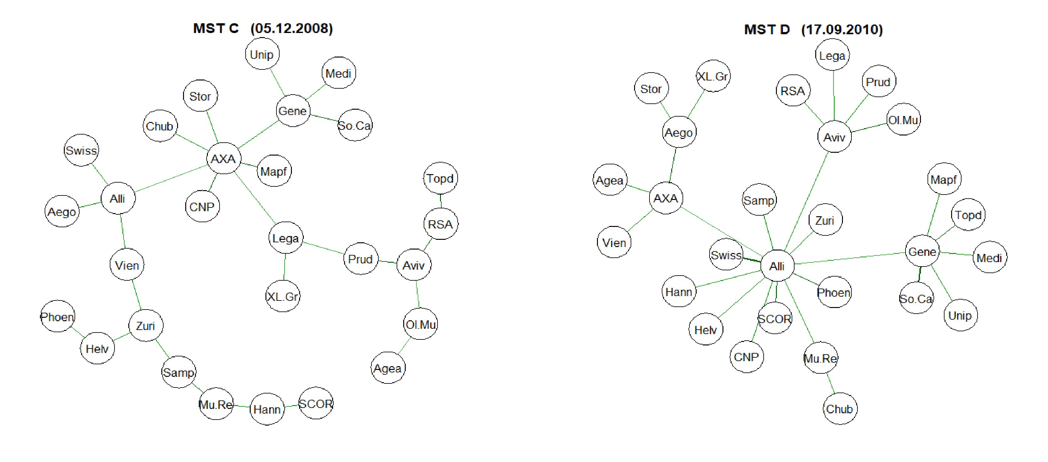
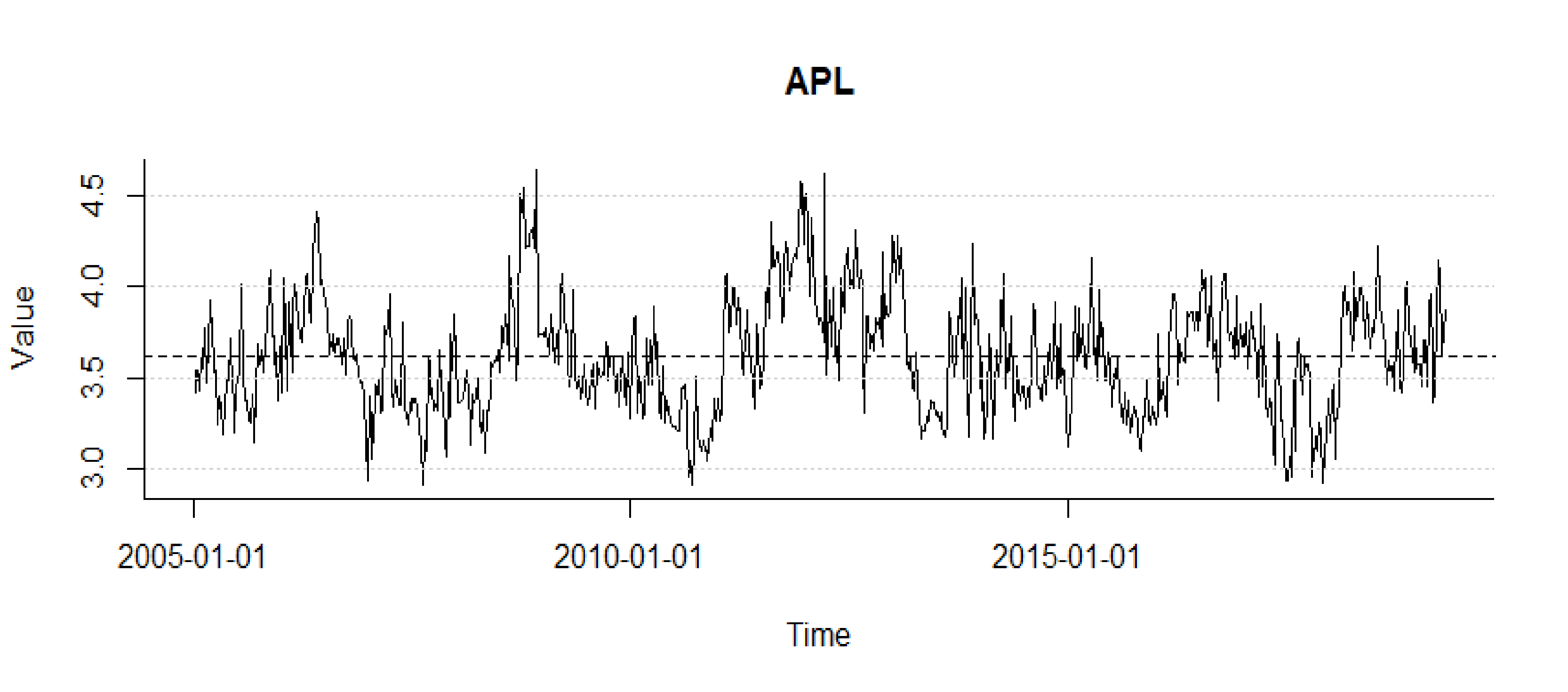
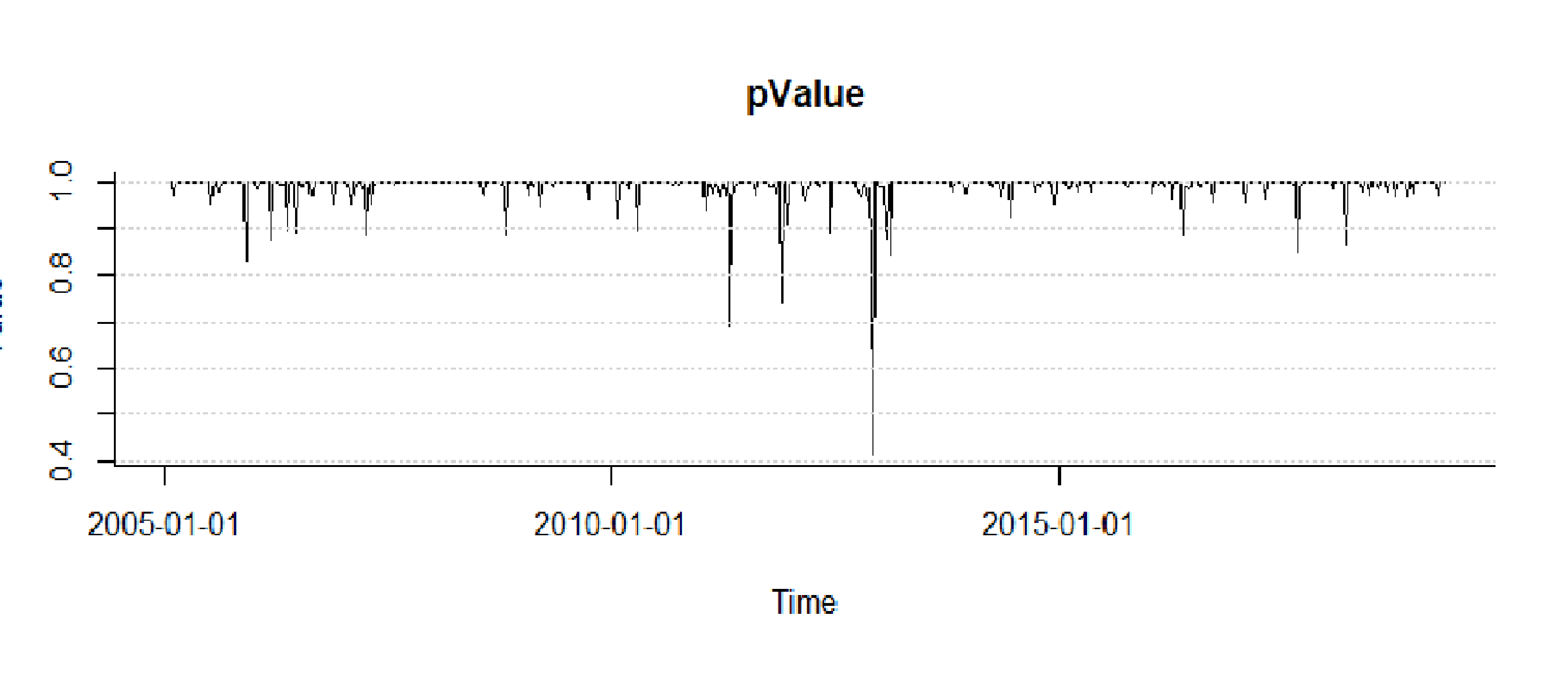
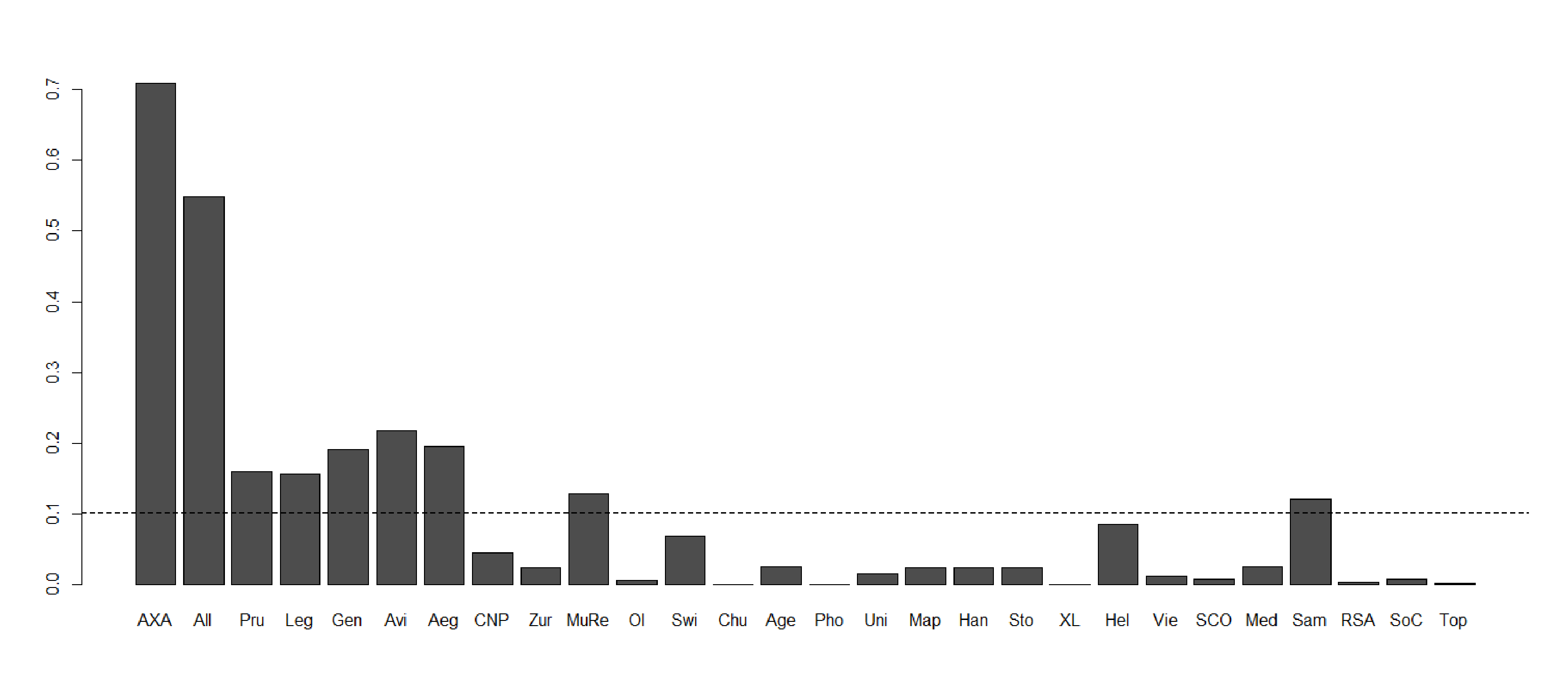
In the second stage the miminum spanning trees obtained were used to determine the time series for: the average path legth (Fig. 2), the maximum degree (Fig. 3), the parameters of the power law of the degree distribution and the corresponding values of pValue (Fig. 4) and the betweeness centrality. The average values of BC for the studied period 07.01.2005–26.04.2019 obtained for the different insurers is shown on Fig. 5. Finally, Figure 6 presents the BC times series only for selected insurers, i.e. for the two having the highest, lowest and ‘average’ mean values of the indicator. The highest values and were obtained for AXA and Allianz, respectively, the lowest (0,000) – for Phoenix, Chubb Ltd and XL.Group, and the ‘average’ mean value of BC is represented by Munich Re.




5. Conclusions
Our aim was to study the dependance and linkage structure, together with its dynamics during the period 07.01.2005–26.04.2019 enclosing the financial crisis of the years 2007–2009 as well as the European public debt crisis of 2010–2012, in the case of the largest European insurance companies and making use of the minimum spanning trees. The correlation coefficients, crucial for the analysis made, were obtained using the estimated two-dimensional copula-DCC-GARCH models, whilst the minimum spanning trees were constructed by means of the Kruskal algorithm. The dependance structure dynamics was studied with the aid of time series for suitably chosen topological indices of the network.
The results lead to the conclusion that the analyzed time series of the topological indices for the minimum spanning trees () constructed using the distances obtained from the dynamical correlations, do not show any trend, but at the same time they show a significant variability.
Looking on the average path length and the maximum degree (cf. Figures 2 and 3) we can determine the periods during which these two indicators are clearly below the average (shown as the dotted line on the two figures), and the periods during which their values are distinctly above average. Moreover, it is apparent that a drop in the APL goes together with a soar of the maximum degree. When the mean distance tends to get smaller, it signalizes a shrinking of the dependances network, i.e. an uplift of the interdependances between the insurance companies which implies also a higher ability of information transfer. A clear shrinking of the network can be seen for the period 02.06.2006--17.08.2007, i.e. precisely just before the subprime crisis and during its first phase44 4 The crisis phases and the developmentsl inked to them are described in details in [10], Appendix A. Timeline of crisis., as well as for the period 05.12.2008–17.09.2010, i.e. just before and at the very beginnning of the European public debt crisis. The minimum spanning trees at the beginning and at the end of these two periods are shown on Fig. 1 (MST A, MST B, MST C, MST D, respectively). On that basis, analyzing the minimum spanning trees structure for the remaining weeks (the corresponding results are available on demand) we can come to the conclusion that during the time of the largest turbulences on global markets, the average distance for the trees is low, while their degree is high. In this kind of trees we can distinguish several crucial insurance companies with a high value of betweenness centrality, i.e. having an important control over the network. As it is apparent from the graphics shown on Fig. 6, during the subprime crisis, the network was controlled essentially by AXA alone, whereas during the European public debt crisis, Allianz took over the control. In general, we can also remark that during the period studied, these are the two companies that gain in turn control over the network.
On the other hand, from the analysis of the time series for the parameters and the corresponding values pValue we can see that in each period studied the degree distribution of follows a power law (see Fig. 4), i.e. the networks are scale-free. Typically, such networks have a small number of vertices with a large number of edges starting from them — these are the hubs — and many vertices with only one edge. From our point of view, this kind of network is seen as ‘favourable’ to the propagation of information (systemic risk) and the companies-hubs are systemically relevant.
In conclusion, we can claim that the scale-free character of the network of relations between the insurers, observed in each period under study, favours the propagation of potential systemic risk in the European insurance sector for which our source is the G-SIIs list of companies. Moreover, due to the shrinkage of the networks during the periods of strong turbulences on financial markets, the ability to propagate significantly increases.
6. Acknowledgements
This article was supported by funds subsided to the Faculty of Finance and Law of the Cracow University of Economics as a support for the research potential.
References
- [1] Baluch F., Mutenga S., Parsons C. Insurance, Systemic Risk and the Financial Crisis, The Geneva Papers on Risk and Insurance - Issues and Practice, Vol. 36(1) (2011), 126-163. doi:10.1057/gpp.2010.40
- [2] Bednarczyk T., Czy sektor ubezpieczeniowy kreuje ryzyko systemowe? (in Polish, Does the insurance sector generate systemic risk?), Studia Oeconomica Posnaniensia, Vol. 11 (260) (2013), 7-17
- [3] Bell M., Keller B., Insurance and Stability: The Reform of Insurance Regulation, Zurich Financial Services Group Working Paper (2009).
- [4] Bierth C., Irresberger F., Weiß G. N.,Systemic risk of insurers around the globe, Journal of Banking & Finance, 55, (2015), 232-245. doi:10.1016/j.jbankfin.2015.02.014
- [5] Billio M., Getmansky M., Lo A. W., Pelizzon L., Econometric measures of connectedness and systemic risk in the finance and insurance sectors, Journal of Financial Economics, Vol. 104(3) (2012), 535-559, doi:10.1016/j.jfineco.2011.12.010
- [6] Chen H., Cummins J. D., Viswanathan K. S., Weiss M. A., Systemic Risk and the Interconnectedness Between Banks and Insurers: An Econometric Analysis, Journal of Risk and Insurance, Vol. 81(3), (2013), 623-652. doi:10.1111/j.1539-6975.2012.01503.x
- [7] Cummins J. D., Weiss M. A., Systemic Risk and The U.S. Insurance Sector, Journal of Risk and Insurance, Vol. 81(3), (2014), 489-528. doi:10.1111/jori.12039
- [8] Czerwińska T., Systemic risk in the insurance sector, Problemy Zarządzania, Vol. 12(48), (2014), 41-63. doi:10.7172/1644-9584.48.3
- [9] EIOPA, Systemic risk and macroprudential policy in insurance, Publications Office of the European Union (2017),
- [10] Geneva Association, Systemic risk in insurance: an analysis of insurance and financial stability, Technical report, Special Report of The Geneva Association Systemic Risk Working Group, Switzerland (2010),
- [11] Harrington S. E., The Financial Crisis, Systemic Risk, and the Future of Insurance Regulation, Journal of Risk and Insurance, Vol. 76(4), (2009), 785-819. doi:10.1111/j.1539-6975.2009.01330.x
- [12] IAIS, Global Systemically Important Insurers: Final Initial Assessment Methodology, International Association of Insurance Supervisors, July 18, Bank for International Settlements, Basel (2013),
- [13] Johnson N. F., McDonald M., Suleman M., Williams S., Howison S., What shakes the FX tree? understanding currency dominance, dependence, and dynamics (keynote address), SPIE Third International Symposium on Fluctuations and Noise, International Society for Optics and Photonics, (2005), 86–99.
- [14] Mantegna R. N., Hierarchical structure in financial markets, The European Physical Journal B-Condensed Matter and Complex Systems, Vol. 11, (1999), 193–197.
- [15] Mantegna R. N., Stanley H. E.,Introduction to econophysics: correlations and complexity in finance, Cambridge university press (1999).
- [16] Marti G., Nielsen, F., Bińkowski M., Donnat P. A review of two decades of correlations, hierarchies, networks and clustering in financial markets, (2017), arXiv preprint arXiv:1703.00485
- [17] Matesanz D., Ortega G. J., Sovereign public debt crisis in europe. a network analysis, Physica A: Statistical Mechanics and its Applications Vol.436, (2015), 756–766.
- [18] Nelson D. B., Conditional Heteroskedasticity in Asset Returns: A New Approach, Econometrica, Vol. 59, (1991), 347–370
- [19] nnela J. P., Chakraborti A., Kaski K., Kertesz J.,Dynamic asset trees and black Monday, Physica A: Statistical Mechanics and its Applications, Vol. 324, (2003) , 247–252.
- [20] Onnela J. P., Chakraborti A., Kaski K., Kertesz J., Kanto A., Dynamics of market correlations: Taxonomy and portfolio analysis, Physical Review E, Vol.68 (2003) , 056-110.
- [21] Onnela J. P., Chakraborti A., Kaski K., Kertesz J., Dynamic asset trees and portfolio analysis, The European Physical Journal B-Condensed Matter and Complex Systems, Vol. 30, (2002), 285–288,
- [22] Patton, A.J.,Modelling asymmetric exchange rate, International Economic Review 47 (2) (2006), 527-556,
- [23] Sensoy A., Tabak B. M., Dynamic spanning trees in stock market networks: The case of Asia-Pacific, Physica A: Statistical Mechanics and its Applications, Vol. 414, (2014), 387–402.
- [24] Tang Y., Xiong J. J., Jia Z.Y., Zhang Y.C., Complexities in financial network topological dynamics: Modeling of emerging and developed stock markets, Complexity Vol. 2018, (2018), article ID 4680140.
- [25] Wanat S., Denkowska A., Measuring systemic risk in the European insurance sector using copula-DCC-GARCH model and selected clustering methods, Conference Proceedings, 36th International Conference Mathematical Methods in Economics, Jindřichův Hradec, September 12-14, 2018, Faculty of Mathematics and Physics Charles University, Praha, ISBN: 978-80-7378-371-6, (2018), 630-635.
- [26] Weiß G. N., Mühlnickel J., Why do some insurers become systemically relevant?, Journal of Financial Stability, Vol. 13, (2014), 95-117.