跳到论文正文
W Papers独立论文阅读器 arXiv:1908.01095 论文正文 计算阅读时间 · 0%
引用这篇论文根据当前论文元数据生成,正式投稿前建议核对。


License: CC BY 4.0
arXiv:1908.01095v2 [quant-ph] 30 Jan 2020

Completely positive master equation for arbitrary driving and small level spacing

Evgeny Mozgunov Affiliation: Center for Quantum Information Science & Technology, University of Southern California, Los Angeles, California 90089, USA    Daniel Lidar Affiliation: Center for Quantum Information Science & Technology, University of Southern California, Los Angeles, California 90089, USA Affiliation: Department of Electrical and Computer Engineering, University of Southern California, Los Angeles, California 90089, USA Affiliation: Department of Chemistry, University of Southern California, Los Angeles, California 90089, USA Affiliation: Department of Physics and Astronomy, University of Southern California, Los Angeles, California 90089, USA
Abstract

Markovian master equations are a ubiquitous tool in the study of open quantum systems, but deriving them from first principles involves a series of compromises. On the one hand, the Redfield equation is valid for fast environments (whose correlation function decays much faster than the system relaxation time) regardless of the relative strength of the coupling to the system Hamiltonian, but is notoriously non-completely-positive. On the other hand, the Davies equation preserves complete positivity but is valid only in the ultra-weak coupling limit and for systems with a finite level spacing, which makes it incompatible with arbitrarily fast time-dependent driving. Here we show that a recently derived Markovian coarse-grained master equation (CGME), already known to be completely positive, has a much expanded range of applicability compared to the Davies equation, and moreover, is locally generated and can be generalized to accommodate arbitrarily fast driving. This generalization, which we refer to as the time-dependent CGME, is thus suitable for the analysis of fast operations in gate-model quantum computing, such as quantum error correction and dynamical decoupling. Our derivation proceeds directly from the Redfield equation and allows us to place rigorous error bounds on all three equations: Redfield, Davies, and coarse-grained. Our main result is thus a completely positive Markovian master equation that is a controlled approximation to the true evolution for any time-dependence of the system Hamiltonian, and works for systems with arbitrarily small level spacing. We illustrate this with an analysis showing that dynamical decoupling can extend coherence times even in a strictly Markovian setting.

1 Introduction

Modeling experiments requires taking into account that physical systems are open, i.e., not ideally isolated from their environments. Usually an environment contains many more degrees of freedom than the system itself, but is not in any interesting phase of matter where the detailed modeling of each of those degrees of freedom is required. This makes the problem of modeling open systems tractable. More precisely, the problem is tractable under a list of assumptions on the parameters of the bath (environment) and its interaction with the system [1, 2, 3].

One natural approach is to consider the case when this interaction is weak compared to all other energy scales in the problem. In this limit, Davies showed [4] that the dynamics of the system are given by a Markovian master equation with what is now called Davies generators. Rigorous bounds on the error between the solution of this equation and the true evolution can be obtained [presented here in Eq. (264)]. The largest contribution to the error comes from making the rotating wave approximation (RWA).11 1 This approximation is stated explicitly in Ref. [3], page 87, around Eq. (3.6.67). After the system evolves for a time set by a relevant relaxation timescale, the error in its density matrix is given by:

system-bath coupling strength×bath correlation time/system level-spacing.\textrm{system-bath coupling strength}\times\penalty\ \sqrt{\textrm{bath correlation time}/\textrm{system level-spacing}}\ . (1)

This quantity, in general, becomes exponentially large in the system size due its denominator, so that the coupling strength or the bath correlation time need to be sufficiently small for the use of Davies generators to be justified, up to some upper system size limit. In practice, for convenience and also because it may apply in a range that is larger than the rigorous but conservative bounds imply, the Lindblad master equation [5] with Davies generators is often used outside its formal range of applicability in modeling of experiments (e.g., Ref. [6, 7, 8, 9]). In such cases it should be understood as a semi-empirical model of open system dynamics, that possesses all the physical properties of the dynamics without reproducing them exactly. Unfortunately, since we naturally wish to apply modeling tools to problems for which we do not know a priori what the correct answer is, this approach cannot provide correctness guarantees. However, other methods are even more susceptible to this problem, e.g., a path-integral (non-master equation) approach based on integrating out the bath [10, 11, 12]: this involves integration over a very high-dimensional space, so methods [13] that bring it back into the realm of numerical feasibility usually involve uncontrollable approximations.

One of the important requirements of open system dynamics is complete positivity [14], under which density matrices whose eigenvalues are by definition non-negative are mapped to other such matrices, even when applied to a subsystem of a larger system.22 2 It should be noted that complete positivity can be relaxed without losing physicality; see, e.g., Ref. [15]. This property is equivalent to the Markovian master equation being in Lindblad canonical form [5, 16]. There are numerous other master equations (e.g., Refs. [17, 18, 19, 20, 21, 22, 23, 24, 25, 26, 27, 28, 29, 30, 31, 32, 33, 34, 35, 36, 37, 38, 39]), some in Lindblad form and some not, whose domains of validity and ranges of applicability were not always studied in detail. One promising candidate is a coarse-grained master equation (CGME) [40], which is in Lindblad form and thus automatically completely positive (CP). In this work we show that a suitably generalized variant of this equation, that includes an arbitrarily time-dependent system Hamiltonian (hence called the “time-dependent CGME”), has a much milder error than (1):

system-bath coupling strength×bath correlation time,\textrm{system-bath coupling strength}\times\textrm{bath correlation time}\ , (2)

which does not diverge with the system size nn for local observables, and has only a polynomial [O⁡(nα)O(n^{\alpha}) with 1/2≤α≤11/2\leq\alpha\leq 1] prefactor for nonlocal observables. We note that the full form of the error estimate (2) is not uniform over the evolution time, unlike some of the error bounds developed elsewhere [39, 41]. We also show that this new master equation is an improvement over the Lindblad equation with Davies generators in that it has a local structure, compatible with approximate simulation methods with asymptotically smaller costs [O⁡(n)O(n) vs. O⁡(exp⁡(n))O(\exp(n))], and that the error estimate (2) is valid for an arbitrary time-dependence of the system Hamiltonian. In particular, the time-dependent CGME is compatible with the assumption of arbitrarily fast gates, often made in the circuit model of quantum computing, e.g., in the analysis of fault-tolerant quantum error correction [42]. This assumption was shown to be incompatible with the derivation of the Davies master equation [43].

This paper is structured as follows. We summarize our main results in Sec. 2, where we present the main master equations involved in this work: Redfield and Davies-Lindblad (well known), and coarse-grained, both time-independent and time-dependent (new). We also present bounds that provide the range of applicability of each type of master equation (new). We show that these bounds can be expressed entirely in terms of only two timescales, namely the fastest system decoherence timescale, and the characteristic timescale of the decay of the bath correlation function. The reader interested only in the results and not in the details of derivations can safely read only this section and then skip to the conclusions in Sec. 7. Derivations begin in Sec. 3, where we present a simple, new derivation of the time-independent CGME. We express the equation in CP (Lindblad) form, state the range of validity for different approximations made in the derivation, and thus for the equation itself. We also compare the range of applicability with other master equations, and note the spatial locality of the Lindblad generators of the CGME. At this point we are ready to address the case of time-dependent Hamiltonians. The derivation of the equation for this case (which happens to result in exactly the same form) is given in Sec. 4. In particular, this equation is well suited for the simulation of open system adiabatic quantum computation, but also for dynamical decoupling, which involves the opposite limit of very fast system dynamics. We note that while we will sometimes refer to qubits, none of the results we discuss in this work are limited to qubits, and in fact any finite multi-level system, or interacting set of such systems, is captured by the formalism. We study some applications and examples in Sec. 5, including error suppression using a dynamical decoupling protocol, and numerical results of the comparison of our master equation with the Redfield and Lindblad-Davies master equations. In the remainder of the paper we derive the range of validity of the various master equations we study. We give a detailed treatment of the Born approximation and the other approximations involved, in terms of rigorous bounds presented in Sec. 6, where we also discuss the generalization to multiple coupling terms and analyze the scaling of the error bounds for large system sizes. Conclusions are presented in Sec. 7. Various additional technical details are given in the Appendix.

2 Three master equations

This section provides a summary of our main results. We first present a brief background to define basic concepts and notation, followed by the definition and properties of the two main timescales we use later to provide bounds and ranges of applicability. We then summarize the three master equations we focus on in this work, followed by upper bounds on the distance of their solutions from the true state.

2.1 Background

Consider a system interacting with its environment as described by the total Hamiltonian

Htot=H⊗Ib+A⊗B+I⊗Hb.H_{\textrm{tot}}=H\otimes I_{\text{b}}+A\otimes B+I\otimes H_{\text{b}}\ . (3)

Here HH is the time-independent system Hamiltonian (we treat the time-dependent case in Sec. 4), HbH_{\text{b}} is the bath Hamiltonian, and AA and BB are, respectively, Hermitian system and bath operators. The more general situation, with V=A⊗BV=A\otimes B replaced by ∑iAi⊗Bi\sum_{i}A_{i}\otimes B_{i}, is easily treated as well (see Sec. 3.7), but we avoid it here to simplify the notation. We choose AA to be dimensionless with ‖A‖=1\|A\|=1 [the operator norm is defined in Eq. (36)] and BB to have energy units, but we deliberately do not set ‖B‖=1\|B\|=1, since we wish to account for baths (such as harmonic oscillator baths) for which ‖B‖\|B\| can be infinite. We also set ℏ≡1\hbar\equiv 1 throughout, so that energy and frequency have identical units.

Let the eigenstates of HH be {|n⟩}\{|n\rangle\} , and the corresponding eigenvalues {En}\{E_{n}\}. Equivalently, H=∑nEn​ΠnH=\sum_{n}E_{n}\Pi_{n}, where Πn\Pi_{n} is a projector onto the eigenspace with eigenvalue EnE_{n}, and Πm​Πn=δm​n​Πn\Pi_{m}\Pi_{n}=\delta_{mn}\Pi_{n}. Note that in the interaction picture A⁡(t)=U†​(t)​A​U​(t)=∑n​mAn​m​e−i​Em​n​t​|n⟩​⟨m|A(t)=U^{\dagger}(t)AU(t)=\sum_{nm}A_{nm}e^{-iE_{mn}t}|n\rangle\langle m| where Em​n=Em−EnE_{mn}=E_{m}-E_{n}, An​m=⟨n|​A​|m⟩A_{nm}=\bra{n}A\ket{m}, and UU is the solution of U˙=−i​H​U\dot{U}=-iHU. Let

Aω=∑m​n:Em​n=ωAn​m|n⟩⟨m|=∑m​n:Em​n=ωΠnAΠm=A−ω†,A_{\omega}=\sum_{mn:E_{mn}=\omega}A_{nm}|n\rangle\langle m|=\sum_{mn:E_{mn}=\omega}\Pi_{n}A\Pi_{m}=A_{-\omega}^{\dagger}\ , (4)

so that33 3 The choice of the sign for this notation, as well as other notation choices, follow the textbook [2], p.133-134.

A⁡(t)=∑ωAω​e−i​ω​t.A(t)=\sum_{\omega}A_{\omega}e^{-i\omega t}\ . (5)

Here ω\omega runs over all the energy differences (Bohr frequencies) between the eigenvalues of HH.

We assume henceforth that the bath is stationary — [ρb,Hb]=0[\rho_{\text{b}},H_{\text{b}}]=0 where ρb\rho_{\text{b}} is the bath state — and introduce the bath correlation function 𝒞⁡(t)\mathcal{C}(t) and its Fourier transform γ⁡(ω)\gamma(\omega), known as the bath spectral density:

𝒞⁡(t)\displaystyle\mathcal{C}(t) =Tr⁡[ρb​B​(t)​B]=𝒞∗​(−t)=12​π​∫−∞∞e−i​ω​t​γ​(ω)​𝑑ω\displaystyle=\mathrm{Tr}[\rho_{\text{b}}B(t)B]=\mathcal{C}^{*}(-t)=\frac{1}{2\pi}\int_{-\infty}^{\infty}e^{-i\omega t}\gamma(\omega)d\omega (6a)
γ⁡(ω)\displaystyle\gamma(\omega) =∫−∞∞𝒞⁡(t)​ei​ω​t​𝑑t=f⁡(ω)+f∗​(ω),\displaystyle=\int_{-\infty}^{\infty}\mathcal{C}(t)e^{i\omega t}dt=f(\omega)+f^{*}(\omega)\ , (6b)

where B⁡(t)=ei​Hb​t​B​e−i​Hb​tB(t)=e^{iH_{\text{b}}t}Be^{-iH_{\text{b}}t} and

f⁡(ω)=∫0∞C⁡(t)​ei​ω​t​𝑑t=12​γ​(ω)+i​S​(ω),S⁡(ω)=12​i​[f⁡(ω)−f∗​(ω)]=S∗​(ω).f(\omega)=\int_{0}^{\infty}C(t)e^{i\omega t}dt=\frac{1}{2}\gamma(\omega)+iS(\omega)\ ,\quad S(\omega)=\frac{1}{2i}\left[f(\omega)-f^{*}(\omega)\right]=S^{*}(\omega)\ . (7)

Note that the real-valued functions S⁡(ω)S(\omega) and γ⁡(ω)\gamma(\omega) are related via a Kramers-Kronig transform

S⁡(ω)=12​π​∫−∞∞𝒫⁡(1ω−ω′)​[γ⁡(ω′)]​d​ω′,S(\omega)=\frac{1}{2\pi}\int_{-\infty}^{\infty}\mathcal{P}\left(\frac{1}{\omega-\omega^{\prime}}\right)[\gamma(\omega^{\prime})]d\omega^{\prime}\ , (8)

where 𝒫⁡(1x)​[f]=limϵ→0∫−ϵϵf⁡(x)x​𝑑x\mathcal{P}\left(\frac{1}{x}\right)[f]=\lim_{\epsilon\to 0}\int_{-\epsilon}^{\epsilon}\frac{f(x)}{x}dx is the Cauchy principal value.44 4 This follows from the identity ∫0∞d​τ​ei​x​τ=π​δ​(x)+i​𝒫​(1x)\int_{0}^{\infty}d\tau e^{ix\tau}=\pi\delta(x)+i\mathcal{P}\left(\frac{1}{x}\right). When A⊗BA\otimes B is replaced by ∑iAi⊗Bi\sum_{i}A_{i}\otimes B_{i}, we note the positivity of γi​j​(ω)=∫d​t​ei​ω​t​Tr​[ρb​Bi​(t)​Bj]\gamma_{ij}(\omega)=\int dte^{i\omega t}\mathrm{Tr}[\rho_{\text{b}}B_{i}(t)B_{j}] as a matrix in the indices i,ji,j (of course this reduces to γ⁡(ω)≥0\gamma(\omega)\geq 0 in the scalar case). This is a non-trivial fact that is usually associated with Bochner’s theorem, as e.g., in the textbook [2]. In Appendix A we give two different proofs, one using Bochner’s theorem and another that is direct. If we assume not only that the bath state is stationary, but that it is also in thermal equilibrium at inverse temperature β\beta, i.e., ρb=e−β​Hb/𝒵\rho_{\text{b}}=e^{-\beta H_{\text{b}}}/\mathcal{Z}, 𝒵=Tr​e−β​Hb\mathcal{Z}=\mathrm{Tr}e^{-\beta H_{\text{b}}}, then it follows that the correlation function satisfies the time-domain Kubo-Martin-Schwinger (KMS) condition [2, 44]:

C⁡(t)=Tr⁡[ρb​B​(0)​B​(t+i​β)].C(t)=\mathrm{Tr}[\rho_{\text{b}}B(0)B(t+i\beta)]\ . (9)

If in addition the correlation function is analytic in the strip between t=−i​βt=-i\beta and t=0t=0, then it follows that the Fourier transform of the bath correlation function satisfies the frequency domain KMS condition [2, 44]:

γ⁡(−ω)=e−β​ω​γ​(ω)​∀ω≥0.\gamma(-\omega)=e^{-\beta\omega}\gamma(\omega)\ \forall\omega\geq 0\ . (10)

We note that the thermal equilibrium assumption is not necessary for the results we derive in this work, and we never use it in our proofs. We mention it here for completeness, and also since we use it in one of our dynamical decoupling examples later on. Finally, note that 𝒞⁡(t)\mathcal{C}(t) has units of frequency squared.

2.2 The bath correlation time τB\tau_{B} and the fastest system decoherence timescale τS​B\tau_{SB}

We define the two key quantities

1τS​B\displaystyle\frac{1}{\tau_{SB}} =∫0∞|𝒞⁡(t)|​𝑑t\displaystyle=\int_{0}^{\infty}|\mathcal{C}(t)|dt (11a)
τB\displaystyle\tau_{B} =∫0Tt​|𝒞⁡(t)|​𝑑t∫0∞|𝒞⁡(t)|​𝑑t\displaystyle=\frac{\int_{0}^{T}t|\mathcal{C}(t)|dt}{\int_{0}^{\infty}|\mathcal{C}(t)|dt} (11b)

Here TT is the total evolution time, used as a cutoff which can often be taken as ∞\infty. We show later that in the interaction picture ‖ρ˙‖1≤4​‖ρ‖1/τS​B\|\dot{\rho}\|_{1}\leq 4\|\rho\|_{1}/\tau_{SB}, where ρ\rho is the system density matrix and the trace norm defined in Eq. (35), so that we can interpret τS​B\tau_{SB} as the fastest system decoherence timescale, or timescale over which ρ\rho changes due to the coupling to the bath, in the interaction picture (i.e., every other system decay timescale, including the standard T1T_{1} and T2T_{2} relaxation and dephasing times, must be longer). The quantity τB\tau_{B} is the characteristic timescale of the decay of 𝒞⁡(t)\mathcal{C}(t). We return in Sec. 6 to why we define these timescales in this manner, but note that Eq. (11b) becomes an identity if we choose |𝒞(t)|∝e−t/τB|\mathcal{C}(t)|\propto e^{-t/\tau_{B}} and take the limit T→∞T\to\infty.

We further note that τS​B\tau_{SB} and τB\tau_{B} are the only two parameters relevant for determining the range of applicability of the various master equations; in particular, nothing about the norm or time-dependence of HtotH_{\text{tot}} affects the accuracy of our time-dependent CGME, given below. In particular, HtotH_{\text{tot}} can be arbitrarily large or small in the operator norm (strong coupling, unbounded bath), or have an arbitrarily large derivative (non-adiabatic regime). This remark is important in light of previous approaches, so we expand on it some more.

In previous work it was common to extract a dimensionful coupling parameter gg, i.e., to replace BB by g​B~g\tilde{B}, where ‖B~‖=1\|\tilde{B}\|=1. One then defines τB=∫0∞|C~​(t)|​𝑑t\tau_{B}=\int_{0}^{\infty}|\tilde{C}(t)|dt in terms of a dimensionless correlation function C~​(t)=C⁡(t)/g2\tilde{C}(t)=C(t)/g^{2} [31]. One problem with this approach is the arbitrariness of distributing the numerical factors between gg and B~\tilde{B}. Another is that it precludes unbounded baths, such as oscillator baths, for which ‖B‖=∞\|B\|=\infty. In contrast, the formalism we present here is applicable even when ‖B‖\|B\| diverges. Furthermore, ‖B‖\|B\| contains an extra scale that does not carry any new information about the range of applicability of the master equations we discuss and derive. By not introducing this extra scale we highlight that there are only two free parameters in our analysis of the error: τB\tau_{B} and τS​B\tau_{SB}, and no other information about the bath is needed. I.e., even though different baths will lead to different equations, our results are universal for any bath with the same values of these two parameters (in fact only their dimensionless ratio matters).

Note that we can relate τB\tau_{B} and τS​B\tau_{SB} to the spectral density. First, using γ⁡(ω)>0\gamma(\omega)>0 and C​(t)=C∗​(−t)C(t)=C^{*}(-t):

γ⁡(ω)=|γ⁡(ω)|≤∫−∞∞|C⁡(t)|​𝑑t=2​∫0∞|C⁡(t)|​𝑑t=2τS​B.\gamma(\omega)=|\gamma(\omega)|\leq\int_{-\infty}^{\infty}|C(t)|dt=2\int_{0}^{\infty}|C(t)|dt=\frac{2}{\tau_{SB}}\ . (12)

The dephasing time T2T_{2} and relaxation time T1T_{1} for a single qubit are usually defined as ∝1/γ⁡(0)\propto 1/\gamma(0) and ∝1/γ⁡(ω)\propto 1/\gamma(\omega) respectively, where ω\omega is the qubit operating frequency (e.g., see Ref. [45]), so we see that τS​B≲T1,T2\tau_{SB}\lesssim T_{1},T_{2}, which illustrates our earlier comment that τS​B\tau_{SB} is the fastest system decoherence time-scale. Second, γ′​(ω)=i​∫−∞∞t​C​(t)​ei​ω​t​𝑑t\gamma^{\prime}(\omega)=i\int_{-\infty}^{\infty}tC(t)e^{i\omega t}dt, so that

|γ′​(ω)|≤∫−∞∞|t|​|C⁡(t)|​𝑑t=2​∫0∞t|C⁡(t)|𝑑t=T→∞2​τBτS​B,|\gamma^{\prime}(\omega)|\leq\int_{-\infty}^{\infty}|t||C(t)|dt=2\int_{0}^{\infty}t|C(t)|dt\stackrel{{\scriptstyle\tiny{T\to\infty}}}{{=}}2\frac{\tau_{B}}{\tau_{SB}}\ , (13)

where the limit is taken in Eq. (11b). And lastly, d​γ​(−ω)d​ω=−d​γ​(ω)d​ω|−ω\frac{d\gamma(-\omega)}{d\omega}=-\frac{d\gamma(\omega)}{d\omega}|_{-\omega}, while differentiating the KMS condition yields d​γ​(−ω)d​ω=−β​e−β​ω​γ​(ω)+e−β​ω​d​γ​(ω)d​ω\frac{d\gamma(-\omega)}{d\omega}=-\beta e^{-\beta\omega}\gamma(\omega)+e^{-\beta\omega}\frac{d\gamma(\omega)}{d\omega}, so that:

γ′​(0)=12​β​γ​(0).\gamma^{\prime}(0)=\frac{1}{2}\beta\gamma(0)\ . (14)

This implies that γ′​(0)>0\gamma^{\prime}(0)>0, so that under the KMS condition (10) we can replace Eq. (13) by

β​γ​(0)≤4​τBτS​B.\beta\gamma(0)\leq 4\frac{\tau_{B}}{\tau_{SB}}\ . (15)

The upper bounds on the approximation errors of all the master equations we present below involves the ratio τB/τS​B\tau_{B}/\tau_{SB} [see, e.g., Eqs. (26)-(28)]. The smallness of this ratio is sufficient for the CGME to be useful, while additional assumptions are required for the Davies-Lindblad equation and some versions of the Redfield equation. It follows from Eq. (15) that for our bound to be small it is necessary that the temperature β−1\beta^{-1} is not too low and/or the spectral density at ω=0\omega=0 (roughly the same as the dephasing rate T2−1T_{2}^{-1}) is not too large. The simple condition β​γ​(0)≪1\beta\gamma(0)\ll 1 already rules out diverging spectral densities such as the case of 1/f1/f noise, though this can be ameliorated by introducing a low-frequency cutoff.

We now present the three master equations, in the Schrödinger picture.

2.3 Redfield master equation

For the derivation see Sec. 3.2. This equation was known earlier than the Davies-Lindblad equation [19], and is often used in quantum chemistry. It is not CP and hence cannot be put in Lindblad form:

ρ˙R​(t)=−i⁡[H,ρR​(t)]+(A​ρR​Af−ρR​Af​A+h.c.),{\dot{\rho}}_{R}(t)=-i[H,\rho_{R}(t)]+(A\rho_{R}A_{f}-\rho_{R}A_{f}A+\textrm{h.c.})\ , (16)

where we defined the “filtered" operator:

Af=∫0∞𝒞⁡(−t)​A​(−t)​𝑑t=∑ωAω​∫0∞𝒞⁡(−t)​ei​ω​t​𝑑t=∑ωf∗​(−ω)​Aω,A_{f}=\int_{0}^{\infty}\mathcal{C}(-t)A(-t)dt=\sum_{\omega}A_{\omega}\int^{\infty}_{0}\mathcal{C}(-t)e^{i\omega t}dt=\sum_{\omega}f^{*}(-\omega)A_{\omega}\ , (17)

where f⁡(ω)f(\omega) is defined in Eq. (7), and we used the subscript RR to denote that the density matrix satisfies the Redfield equation (we use a similar subscript notation below to distinguish the solutions of different master equations). There is no natural way to separate the Lamb shift. One of the benefits of the Redfield equation is that there is only one generator AfA_{f} per interaction with the environment A⊗BA\otimes B. We will show that as long as it preserves positivity, the Redfield equation is more accurate than the Davies-Lindblad master equation.

2.4 Davies-Lindblad master equation

For the derivation see Sec. 3.3. This is the familiar result [4]

ρ˙D​(t)\displaystyle{\dot{\rho}}_{D}(t) =−i⁡[H+HLS,ρD]+∑ωγ⁡(ω)​(Aω​ρD​Aω†−12​{ρD,Aω†​Aω}),\displaystyle=-i[H+H_{\mathrm{LS}},\rho_{D}]+\sum_{\omega}\gamma(\omega)(A_{\omega}\rho_{D}A^{\dagger}_{\omega}-\frac{1}{2}\{\rho_{D},A^{\dagger}_{\omega}A_{\omega}\})\ , (18a)
HLS\displaystyle H_{\mathrm{LS}} =−∑ωS(ω)Aω†Aω,S(ω)=12​i∫−∞∞sgn(t)𝒞(t)ei​ω​tdt,\displaystyle=-\sum_{\omega}S(\omega)A^{\dagger}_{\omega}A_{\omega}\ ,\quad S(\omega)=\frac{1}{2i}\int_{-\infty}^{\infty}\sgn(t)\mathcal{C}(t)e^{i\omega t}dt\ , (18b)

where HLSH_{\mathrm{LS}} is the Lamb shift. We note that ad hoc forms of the Lindblad equation are often written down and used without justification, e.g., with just one Lindblad term per qubit (e.g., σ−\sigma_{-} or I−σzI-\sigma_{z} [46, 47]). In reality the Davies generators are derived from first principles, i.e., from the description of the total Hamiltonian of the system and bath. The number of Davies generators is unfortunately exponential in the number of qubits nn: ∑ω\sum_{\omega} is over all 4n4^{n} energy differences.

2.5 Coarse-grained master equation (CGME) for time-independent or time-dependent system Hamiltonians

This is our main new set of results, generalizing Ref. [40] to the time-dependent case.

2.5.1 The time-independent case

For the derivation see Sec. 3.4. First, considering time-independent system Hamiltonians, we obtain:

ρ˙C​(t)=−i⁡[H+HLS,ρC​(t)]+∫−∞∞d​ϵ​(Aϵ​ρC​(t)​Aϵ†−12​{ρC​(t),Aϵ†​Aϵ}),{\dot{\rho}}_{C}(t)=-i[H+H_{\mathrm{LS}},\rho_{C}(t)]+\int_{-\infty}^{\infty}d\epsilon\left(A_{\epsilon}\rho_{C}(t)A_{\epsilon}^{\dagger}-\frac{1}{2}\left\{\rho_{C}(t),A_{\epsilon}^{\dagger}A_{\epsilon}\right\}\right)\ , (19)

where the Lindblad operators are

Aϵ\displaystyle A_{\epsilon} =γ⁡(ϵ)2​π​Ta∫−Ta/2Ta/2ei​ϵ​tA(t)dt\displaystyle=\sqrt{\frac{\gamma(\epsilon)}{2\pi T_{a}}}\int_{-T_{a}/2}^{T_{a}/2}e^{i\epsilon t}A(t)dt (20a)
=∑ωf⁡(ϵ,ω)​Aω,f⁡(ϵ,ω)=γ⁡(ϵ)​Ta2​π​sinc​[Ta​(ϵ−ω)/2],\displaystyle=\sum_{\omega}f(\epsilon,\omega)A_{\omega}\ ,\quad f(\epsilon,\omega)=\sqrt{\frac{\gamma(\epsilon)T_{a}}{2\pi}}\textrm{sinc}[T_{a}(\epsilon-\omega)/2]\ , (20b)

with sinc⁡(x)≡sin⁡(x)/x\sinc(x)\equiv\sin(x)/x, and where TaT_{a} is the averaging, or coarse-graining time, discussed below. The continuous family of terms labeled by ϵ\epsilon is an unusual form of the Lindblad equation, but is manifestly CP. The more standard form in terms of a discrete sum over transition frequencies is equivalent to this one, and is given in Eq. (71) below. The range of applicability of the CGME is only slightly smaller than that of the Redfield ME, as we discuss in Sec. 3.5. Much like for Davies generators, there are exponentially many frequency differences, but unlike the Davies case the discretization of the continuous integral ∫𝑑ϵ\int d\epsilon makes it possible to keep the number of generators constant in the system size for each A⊗BA\otimes B term. These results are presented in Sec. 3.6.

The same applies for the Lamb shift, which is

HLS\displaystyle H_{\mathrm{LS}} =∑ω​ω′Fω​ω′​Aω′​Aω\displaystyle=\sum_{\omega\omega^{\prime}}F_{\omega\omega^{\prime}}A_{\omega^{\prime}}A_{\omega} (21a)
Fω​ω′\displaystyle F_{\omega\omega^{\prime}} =12​Ta​ω+​Re​∫0Tad​θ​(ei⁡(ω​θ−Ta​ω+)−e−i⁡(ω′​θ−Ta​ω+))​𝒞​(θ)=Fω​ω′∗=F−ω′,−ω,\displaystyle=\frac{1}{2T_{a}\omega_{+}}\textrm{Re}\int_{0}^{T_{a}}d\theta\left(e^{i(\omega\theta-T_{a}\omega_{+})}-e^{-i(\omega^{\prime}\theta-T_{a}\omega_{+})}\right)\mathcal{C}(\theta)=F_{\omega\omega^{\prime}}^{*}=F_{-\omega^{\prime},-\omega}\ , (21b)

where ω+=ω+ω′2\omega_{+}=\frac{\omega+\omega^{\prime}}{2}. Note that Fω​ω′F_{\omega\omega^{\prime}} is well defined in the limit ω+→0\omega_{+}\to 0. The results above are generalized to the nn-qubit setting in Sec. 3.7.

2.5.2 The time-dependent case

For the derivation see Sec. 4. In the case of a time-dependent system Hamiltonian H⁡(t)H(t) we obtain the same form, and even the same range of applicability, except that all the operators are now time-dependent:

ρ˙C​(t)=−i⁡[H⁡(t)+HLS​(t),ρC]+∫−∞∞d​ϵ​(Aϵ​(t)​ρC​Aϵ†​(t)−12​{ρC,Aϵ†​(t)​Aϵ​(t)}),{\dot{\rho}}_{C}(t)=-i[H(t)+H_{\mathrm{LS}}(t),\rho_{C}]+\int_{-\infty}^{\infty}d\epsilon\left(A_{\epsilon}(t)\rho_{C}A_{\epsilon}^{\dagger}(t)-\frac{1}{2}\left\{\rho_{C},A_{\epsilon}^{\dagger}(t)A_{\epsilon}(t)\right\}\right)\ , (22)

where the time-dependent Lindblad operators are

Aϵ(t)=γ⁡(ϵ)2​π​Ta∫−Ta/2Ta/2ei​ϵ​t1A(t+t1,t)dt1,A_{\epsilon}(t)=\sqrt{\frac{\gamma(\epsilon)}{2\pi T_{a}}}\int_{-T_{a}/2}^{T_{a}/2}e^{i\epsilon t_{1}}A(t+t_{1},t)dt_{1}\ , (23)

where A⁡(t′,t)=U†​(t′,t)​A​U​(t′,t)A(t^{\prime},t)=U^{\dagger}(t^{\prime},t)AU(t^{\prime},t) with U(t′,t)=𝒯exp[−i∫tt′H(s)ds]U(t^{\prime},t)=\mathcal{T}\exp[-i\int_{t}^{t^{\prime}}H(s)ds] (the forward time-ordered exponential, from t′t^{\prime} on the left to tt on the right), and the time-dependent Lamb shift is

HLS(t)=i2​Ta∫−Ta/2Ta/2dt1∫−Ta/2Ta/2dt2sgn(t1−t2)𝒞(t2−t1)A(t+t2,t)A(t+t1,t).H_{\mathrm{LS}}(t)=\frac{i}{2T_{a}}\int_{-T_{a}/2}^{T_{a}/2}dt_{1}\int_{-T_{a}/2}^{T_{a}/2}dt_{2}\sgn(t_{1}-t_{2})\mathcal{C}(t_{2}-t_{1})A(t+t_{2},t)A(t+t_{1},t)\ . (24)

Although the coarse-graining time TaT_{a} is a free parameter, we show that to minimize the upper bound we derive on the distance between the solutions of the Redfield and coarse-grained master equations it is nearly optimal to choose

Ta=τS​B​τB/5.T_{a}=\sqrt{\tau_{SB}\tau_{B}/5}\ . (25)

2.6 Error bounds and range of applicability

The error bound of the Redfield master equation is

‖ρtrue​(t)−ρR​(t)‖1≤O⁡(τBτS​B​e12​t/τS​B)​ln​(τS​BτB),\|\rho_{\text{true}}(t)-\rho_{R}(t)\|_{1}\leq O\left(\frac{\tau_{B}}{\tau_{SB}}e^{12t/\tau_{SB}}\right)\text{ln}\left(\frac{\tau_{SB}}{\tau_{B}}\right)\ , (26)

where ρtrue​(t)\rho_{\text{true}}(t) denotes the true (approximation-free) state.

The error bound of the Davies-Lindblad master equation is

‖ρtrue​(t)−ρD​(t)‖1≤O⁡((τBτS​B+1τS​B​δ​E)​e12​t/τS​B),\|\rho_{\text{true}}(t)-\rho_{D}(t)\|_{1}\leq O\left(\left(\frac{\tau_{B}}{\tau_{SB}}+\frac{1}{\sqrt{\tau_{SB}\delta E}}\right)e^{12t/\tau_{SB}}\right)\ , (27)

where δ​E=\delta E=mini≠j|Ei−Ej|{}_{i\neq j}|E_{i}-E_{j}| is the level spacing, with EiE_{i} the eigenenergies of the system Hamiltonian HH.

The error bound of both the time-independent and time-dependent coarse-grained master equation is:55 5 Strictly, our proof is only for the time-independent case, but there do not seem to be any obstacles for its generalization to the time-dependent case.

‖ρtrue​(t)−ρC​(t)‖1≤O⁡(τBτS​B​e6​t/τS​B).\displaystyle\|\rho_{\text{true}}(t)-\rho_{C}(t)\|_{1}\leq O\left(\sqrt{\frac{\tau_{B}}{\tau_{SB}}}e^{6t/\tau_{SB}}\right)\ . (28)

In the above expressions, O⁡(X)O(X) is understood for X→0X\to 0, specifically for CGME X=τB/τS​B​e6​t/τS​BX=\sqrt{\tau_{B}/\tau_{SB}}e^{6t/\tau_{SB}}. There is a subtlety in the definition of big-OO notation that we would like to emphasize. By definition, “f⁡(X)=O⁡(X)f(X)=O(X) at X→0X\to 0” means there exist X0,MX_{0},M s.t. for any X≤X0X\leq X_{0} we have f⁡(X)≤M​Xf(X)\leq MX. Applying this to Eq. (28), we have the following unpacking of the above statement: there exist universal constants x0,Mx_{0},M such that if τB/τS​B≤X0\sqrt{\tau_{B}/\tau_{SB}}\leq X_{0} and t≤(τS​B/6)​ln​(X0/τB/τS​B)t\leq(\tau_{SB}/6)\text{ln}(X_{0}/\sqrt{\tau_{B}/\tau_{SB}}), then ‖ρtrue​(t)−ρC​(t)‖1≤M​τB/τS​B​e6​t/τS​B\|\rho_{\text{true}}(t)-\rho_{C}(t)\|_{1}\leq M\sqrt{\tau_{B}/\tau_{SB}}e^{6t/\tau_{SB}} holds. Note that for sufficiently small τB/τS​B\tau_{B}/\tau_{SB}, a dimensionless quantity t/τS​Bt/\tau_{SB} can have an arbitrarily large constant value in this bound. The error can be made arbitrarily small at any fixed value of t/τS​Bt/\tau_{SB} just by choosing a sufficiently small τB/τS​B\tau_{B}/\tau_{SB}. This is what is commonly referred to as the weak coupling limit. We emphasize that the constants X0,MX_{0},M involved in this statement are universal, i.e. independent of the parameters of the equation such as the Hamiltonian and the initial state. In that sense, our bound is uniform. It does depend on time tt as explicitly stated, so it is not uniform in time.66 6 Note that in both the Davies-Lindblad and CGME cases the l.h.s. is bounded above by 22 due to the positivity of the density matrices; this is not necessarily true in the Redfield case. Thus, comparing these bounds, we observe that the Redfield bound is the tightest, which is natural given that it involves the fewest approximations. However, recall that the Redfield master equation is not CP. When comparing the bounds on the solutions of the two CP master equations, we observe that unlike the Davies-Lindblad equation the CGME does not involve the energy gap, which means that the CGME in principle has a much larger range of applicability, in particular for systems whose gap shrinks with growing system size.77 7 By range of applicability we mean the range of parameters over which the approximation is accurate. This range can be defined formally in terms of an upper bound on the right-hand side (r.h.s.), e.g., τB/τS​B​e6​t/τS​B<ϵ\sqrt{{\tau_{B}}/{\tau_{SB}}}e^{6t/\tau_{SB}}<\epsilon for some fixed ϵ<1\epsilon<1.

While the equations and inequalities can be derived for any bath, we made some extra assumptions to prove the error bounds as presented above. Specifically, we assumed a Gaussian bath and the convergence of our series expansion for the Born error, as defined and discussed in detail in Sec. 6.2. For a non-Gaussian bath, extra time scales relating to higher correlation functions generally appear, and the error bound can be derived by a straightforward generalization of our approach. It will contain, besides τB\tau_{B} and τS​B\tau_{SB}, additional terms involving those time scales.

3 (Re-)Derivation of the coarse-grained master equation

Our goal in this section is to present a compact and simplified derivation of the CGME found in Ref. [40]. This master equation is in Lindblad form but avoids making use of the RWA, which contributes the largest approximation error. Instead, the key idea is to introduce a coarse-graining (averaging) timescale, first exploited in this context in Refs. [20, 22]. In this section we consider the case of a time-independent system Hamiltonian, and later generalize our derivation to the time-dependent case, which includes adiabatic evolution as a special case.

Along the way we also derive the Redfield and Davies-Lindblad master equations.

3.1 Setting up

We start from the total Hamiltonian given in Eq. (3), and let V=A⊗BV=A\otimes B. Recall that AA is dimensionless and BB has units of energy. The first few steps in our derivation are standard [2]. In the double system-bath interaction picture V⁡(t)=U0†​(t)​V​U0​(t)V(t)=U_{\textrm{0}}^{\dagger}(t)VU_{\textrm{0}}(t) [where U0U_{\textrm{0}} is the solution of U˙0=−i⁡(H⊗Ib+I⊗Hb)​U0,U0​(0)=1\dot{U}_{\textrm{0}}=-i(H\otimes I_{\text{b}}+I\otimes H_{\text{b}})U_{\textrm{0}},\penalty\ U_{0}(0)=1], and the state satisfies

ρ˙tot​(t)\displaystyle{\dot{\rho}}_{\text{tot}}(t) =−i⁡[V⁡(t),ρtot​(t)]\displaystyle=-i[V(t),\rho_{\text{tot}}(t)] (29a)
ρtot​(t)\displaystyle\rho_{\text{tot}}(t) =ρtot​(0)−i​∫0t[V⁡(τ),ρtot​(τ)]​𝑑τ.\displaystyle=\rho_{\text{tot}}(0)-i\int_{0}^{t}[V(\tau),\rho_{\text{tot}}(\tau)]d\tau. (29b)

Substituting this back into the original equation yields:

ρ˙tot​(t)=−i⁡[V⁡(t),ρtot​(0)]−[V⁡(t),∫0t[V⁡(τ),ρtot​(τ)]]​𝑑τ.{\dot{\rho}}_{\text{tot}}(t)=-i[V(t),\rho_{\text{tot}}(0)]-[V(t),\int_{0}^{t}[V(\tau),\rho_{\text{tot}}(\tau)]]d\tau. (30)

The reduced system state in the interaction picture is defined as ρtrue,I​(t)=Trb​[ρtot​(t)]\rho_{\textrm{true},I}(t)=\mathrm{Tr}_{\text{b}}[\rho_{\text{tot}}(t)], where the subscript “true" denotes that this is the correct, completely approximation-free state. The corresponding true system state in the Schrödinger picture is ρtrue=U0​(t)​ρtrue,I​U0†​(t)\rho_{\textrm{true}}=U_{0}(t)\rho_{\textrm{true},I}U^{\dagger}_{0}(t). The Born approximation,

ρtot​(t)=ρtrue,I​(t)⊗ρb+δ​ρtot,\rho_{\text{tot}}(t)=\rho_{\textrm{true,I}}(t)\otimes\rho_{\text{b}}+\delta\rho_{\text{tot}}, (31)

together with the shift of BB such that Tr⁡[ρb​B]=0\mathrm{Tr}[\rho_{\text{b}}B]=0 allows one to write:

ρ˙true,I​(t)=−Trb​[A⁡(t)⊗B⁡(t),∫0t[A⁡(τ)⊗B⁡(τ),ρtrue,I​(τ)⊗ρb]]​𝑑τ+ℰB,{\dot{\rho}}_{\textrm{true},I}(t)=-\mathrm{Tr}_{\text{b}}[A(t)\otimes B(t),\int_{0}^{t}[A(\tau)\otimes B(\tau),\rho_{\textrm{true,I}}(\tau)\otimes\rho_{\text{b}}]]d\tau+\mathcal{E}_{B}\ , (32)

which can be understood as the definition of the Born approximation error ℰB\mathcal{E}_{B}:

ℰB≡ρ˙true,I​(t)+Trb​[A⁡(t)⊗B⁡(t),∫0t[A⁡(τ)⊗B⁡(τ),ρtrue,I​(τ)⊗ρb]]​𝑑τ,‖ℰB‖1=O⁡(τBτS​B2).\mathcal{E}_{B}\equiv{\dot{\rho}}_{\textrm{true},I}(t)+\mathrm{Tr}_{\text{b}}[A(t)\otimes B(t),\int_{0}^{t}[A(\tau)\otimes B(\tau),\rho_{\textrm{true,I}}(\tau)\otimes\rho_{\text{b}}]]d\tau,\quad\|\mathcal{E}_{B}\|_{1}=O\left(\frac{\tau_{B}}{\tau_{SB}^{2}}\right)\ . (33)

Henceforth we assume that the bath correlation function decays rapidly, namely that τB≪τS​B\tau_{B}\ll\tau_{SB}, where τS​B\tau_{SB} and τB\tau_{B} were defined in Eq. (11).

Now, let ρB,I\rho_{B,I} denote the solution of the master equation after the Born approximation:

ρ˙B,I​(t)=−Trb​[A⁡(t)⊗B⁡(t),∫0t[A⁡(τ)⊗B⁡(τ),ρB​(τ)⊗ρb]]​𝑑τ.{\dot{\rho}}_{B,I}(t)=-\mathrm{Tr}_{\text{b}}[A(t)\otimes B(t),\int_{0}^{t}[A(\tau)\otimes B(\tau),\rho_{B}(\tau)\otimes\rho_{\text{b}}]]d\tau\ . (34)

Later we collect other errors as letters next to BB. The error estimate given in Eq. (33) for ‖ℰB‖1\|\mathcal{E}_{B}\|_{1} is derived in Sec. 6.2 [Eq. (198b)].

We digress briefly to carefully explain the meaning of the norms and big-OO notation used here, since this is important for the remainder of this work. ℰB\mathcal{E}_{B} is an operator acting on the system Hilbert space. The trace norm ‖A‖1\|A\|_{1} is:

‖A‖1≡Tr​A†​A\|A\|_{1}\equiv\mathrm{Tr}\sqrt{A^{\dagger}A} (35)

The operator norm ‖X‖\|X\| is defined as follows:

‖X‖=maxi⁡λX,i\|X\|=\max_{i}\lambda_{X,i} (36)

where λX,i\lambda_{X,i} are the eigenvalues of |X|≡X†​X|X|\equiv\sqrt{X^{\dagger}X} (singular values of XX) indexed by ii. The big-OO notation ℰ=O⁡(x)\mathcal{E}=O(x) is taken for times such that t/τS​B≤Mt/\tau_{SB}\leq M and x→0x\to 0, i.e., there exist an MM-dependent number ϵM\epsilon_{M} and an MM-dependent constant CMC_{M} such that for any x<ϵMx<\epsilon_{M} the error ‖ℰ‖1≤CM​x\|\mathcal{E}\|_{1}\leq C_{M}x.

It is natural to use the trace norm for density matrices. Indeed, if we want to find the deviation in an observable OO relative to the difference between two states, δ​ρ=ρ1−ρ2\delta\rho=\rho_{1}-\rho_{2}, then

|Tr​O​δ​ρ|≤2n​‖O‖​‖δ​ρ‖,|Tr​O​δ​ρ|≤‖O‖​‖δ​ρ‖1.|\mathrm{Tr}O\delta\rho|\leq 2^{n}\|O\|\|\delta\rho\|,\quad|\mathrm{Tr}O\delta\rho|\leq\|O\|\|\delta\rho\|_{1}\ . (37)

The second expression gives a tighter bound, if we manage to have the same bound on ‖δ​ρ‖1\|\delta\rho\|_{1} as on ‖δ​ρ‖\|\delta\rho\|. Fortunately, this will turn out to be the case in this work, and was already observed for the Markov error in Ref. [31]. The key property used to prove the inequality above is submultiplicativity, valid for any unitarily invariant norm [48]:

‖A​B‖1≤‖A‖​‖B‖1.\|AB\|_{1}\leq\|A\|\|B\|_{1}\ . (38)

For simplicity, we assume the bath state to be stationary, such that 𝒞⁡(t,t′)=Tr⁡[ρB​B​(t)​B​(t′)]\mathcal{C}(t,t^{\prime})=\mathrm{Tr}[\rho_{B}B(t)B(t^{\prime})] is invariant with respect to shifts in time of both arguments.88 8 The derivation can potentially be extended to the general case of a two-time correlation function, i.e., without assuming translational invariance; indeed the derivation in [40] does not. We can then replace 𝒞⁡(t,t′)\mathcal{C}(t,t^{\prime}) by 𝒞⁡(t)=Tr⁡[ρB​B​(t)​B]\mathcal{C}(t)=\mathrm{Tr}[\rho_{B}B(t)B], as in Eq. (6a). Recall that 𝒞∗​(t)=𝒞​(−t)\mathcal{C}^{*}(t)=\mathcal{C}(-t). After expanding the commutators, one arrives at

ρ˙B,I​(t)=∫0t𝒞⁡(τ−t)​[A⁡(t)​ρB,I​(τ)​A​(τ)−ρB,I​(τ)​A​(τ)​A​(t)]​𝑑τ+h.c.≡∫0tKt−τB,2​(ρB,I​(τ))​𝑑τ,{\dot{\rho}}_{B,I}(t)=\int_{0}^{t}\mathcal{C}(\tau-t)[A(t)\rho_{B,I}(\tau)A(\tau)-\rho_{B,I}(\tau)A(\tau)A(t)]d\tau+\textrm{h.c.}\equiv\int_{0}^{t}K^{B,2}_{t-\tau}(\rho_{B,I}(\tau))d\tau\ , (39)

where Kt−τB,2K^{B,2}_{t-\tau} is a superoperator. Taking the trace norm, we note that:

‖ρ˙B,I‖1≤4​cB​∫0∞|𝒞⁡(t)|​𝑑t=4​cB/τS​B,\|\dot{\rho}_{B,I}\|_{1}\leq 4c_{B}\int_{0}^{\infty}|\mathcal{C}(t)|dt=4c_{B}/\tau_{SB}, (40)

where we used our earlier choice of setting ‖A‖=1\|A\|=1, and the constant cBc_{B} is chosen as an upper bound on ‖ρB,I‖1\|\rho_{B,I}\|_{1} (if this were a CP map, cB=1c_{B}=1 would hold). Under the condition ∀t,‖ρtest​(t)‖1=1\forall t,\penalty\ \|\rho_{\text{test}}(t)\|_{1}=1 we have

‖∫0tKt−τB,2​(ρtest​(t))​𝑑τ‖1≤4/τS​B.\left\|\int_{0}^{t}K^{B,2}_{t-\tau}(\rho_{\text{test}}(t))d\tau\right\|_{1}\leq 4/\tau_{SB}\ . (41)

We next introduce the Markov approximation ρB,I​(τ)↦ρB,I​(t)\rho_{B,I}(\tau)\mapsto\rho_{B,I}(t):

ρ˙B,I​(t)\displaystyle{\dot{\rho}}_{B,I}(t) =∫0t𝒞⁡(τ−t)​[A⁡(t)​ρB,I​(t)​A​(τ)−ρB,I​(t)​A​(τ)​A​(t)]​𝑑τ+h.c.+ℰM,‖ℰM‖1=O⁡(τBτS​B2)\displaystyle=\int_{0}^{t}\mathcal{C}(\tau-t)[A(t)\rho_{B,I}(t)A(\tau)-\rho_{B,I}(t)A(\tau)A(t)]d\tau+\textrm{h.c.}+\mathcal{E}_{M},\quad\|\mathcal{E}_{M}\|_{1}=O\left(\frac{\tau_{B}}{\tau_{SB}^{2}}\right) (42a)
ρ˙B​M,I​(t)\displaystyle{\dot{\rho}}_{BM,I}(t) =∫0t𝒞⁡(τ−t)​[A⁡(t)​ρB​M,I​(t)​A​(τ)−ρB​M,I​(t)​A​(τ)​A​(t)]​𝑑τ+h.c.=ℒtB​M,I​(ρB​M,I​(t))\displaystyle=\int_{0}^{t}\mathcal{C}(\tau-t)[A(t)\rho_{BM,I}(t)A(\tau)-\rho_{BM,I}(t)A(\tau)A(t)]d\tau+\textrm{h.c.}=\mathcal{L}^{BM,I}_{t}(\rho_{BM,I}(t)) (42b)
∀t,‖ρtest‖1=1:‖ℒtB​M,I​(ρtest)‖1≤4/τS​B\displaystyle\qquad\qquad\qquad\qquad\qquad\qquad\qquad\qquad\forall t,\penalty\ \|\rho_{\text{test}}\|_{1}=1:\penalty\ \|\mathcal{L}^{BM,I}_{t}(\rho_{\text{test}})\|_{1}\leq 4/\tau_{SB} (42c)

Equation (42b) is the Redfield equation [2], which is notoriously non-CP (though various fixes have been proposed [49, 28]). The Markov approximation error ℰM\mathcal{E}_{M} is of same order as the Born approximation error given in Eq. (33) (for more detail see Sec. 6).

We note that the errors on the r.h.s. are not generally additive: if we try to write a Markovian master equation for the true (approximation-free) evolution ρtrue,I\rho_{\text{true},I}, then the error on the r.h.s. will, besides ℰB+ℰM\mathcal{E}_{B}+\mathcal{E}_{M}, contain a correction to the Markov error from the Born error:

ρ˙true,I​(t)=∫0t𝒞⁡(τ−t)​[A⁡(t)​ρtrue,I​(t)​A​(τ)−ρtrue,I​(t)​A​(τ)​A​(t)]​𝑑τ+h.c.+ℰB+ℰM​(ρtrue),\displaystyle{\dot{\rho}}_{\text{true},I}(t)=\int_{0}^{t}\mathcal{C}(\tau-t)[A(t)\rho_{\text{true},I}(t)A(\tau)-\rho_{\text{true},I}(t)A(\tau)A(t)]d\tau+\textrm{h.c.}+\mathcal{E}_{B}+\mathcal{E}_{M}(\rho_{\text{true}}), (43a)
ℰM​(ρtrue)≠ℰM\displaystyle\mathcal{E}_{M}(\rho_{\text{true}})\neq\mathcal{E}_{M} (43b)

In this particular case, using methods from Section 6 the difference between bounds on ‖ℰM​(ρtrue)‖1\|\mathcal{E}_{M}(\rho_{\text{true}})\|_{1} and ‖ℰM‖1\|\mathcal{E}_{M}\|_{1} can be found to be subleading in τB/τS​B\tau_{B}/\tau_{SB}. Since we wish to present higher orders of the error, we do not attempt to collect errors as in Eq. (43a). Instead, our derivation will present a sequence of equations, e.g., ρtrue,ρB,ρB​M\rho_{\text{true}},\rho_{B},\rho_{BM}, and an error estimate for each step.

After using Eq. (5), i.e., in the frequency representation, Eq. (42b) takes the following form:

ρ˙B​M,I​(t)=∑ω,ω′∫0td​τ​𝒞​(τ−t)​e−i⁡(ω​t+ω′​τ)​(Aω​ρB​M,I​Aω′−ρB​M,I​Aω′​Aω)+h.c.{\dot{\rho}}_{BM,I}(t)=\sum_{\omega,\omega^{\prime}}\int_{0}^{t}d\tau\mathcal{C}(\tau-t)e^{-i(\omega t+\omega^{\prime}\tau)}(A_{\omega}\rho_{BM,I}A_{\omega^{\prime}}-\rho_{BM,I}A_{\omega^{\prime}}A_{\omega})+\textrm{h.c.} (44)

We sometimes omit the explicit time dependence of ρ\rho on the r.h.s. since it is always ρ⁡(t)\rho(t) from hereon.

3.2 Redfield master equation

Let us digress briefly in order to establish the form of the Redfield equation presented in Sec. 2. Rotating Eq. (42b) back to the Schrödinger picture we obtain:

ρ˙B​M​(t)=−i⁡[H,ρB​M​(t)]+∫0t𝒞⁡(τ−t)​[A​ρB​M​(t)​A​(τ−t)−ρB​M​(t)​A​(τ−t)​A]​𝑑τ+h.c.{\dot{\rho}}_{BM}(t)=-i[H,\rho_{BM}(t)]+\int_{0}^{t}\mathcal{C}(\tau-t)[A\rho_{BM}(t)A(\tau-t)-\rho_{BM}(t)A(\tau-t)A]d\tau+\textrm{h.c.} (45)

Introducing a new integration variable t′=t−τt^{\prime}=t-\tau:

ρ˙B​M​(t)=−i⁡[H,ρB​M​(t)]+∫0t𝒞⁡(−t′)​[A​ρB​M​(t)​A​(−t′)−ρB​M​(t)​A​(−t′)​A]​d​t′+h.c.{\dot{\rho}}_{BM}(t)=-i[H,\rho_{BM}(t)]+\int_{0}^{t}\mathcal{C}(-t^{\prime})[A\rho_{BM}(t)A(-t^{\prime})-\rho_{BM}(t)A(-t^{\prime})A]dt^{\prime}+\textrm{h.c.} (46)

We extend the upper integration limit from tt to ∞\infty, which introduces an additional error:

ρ˙B​M​(t)\displaystyle{\dot{\rho}}_{BM}(t) =−i⁡[H,ρB​M​(t)]+∫0∞𝒞⁡(−t′)​[A​ρB​M​(t)​A​(−t′)−ρB​M​(t)​A​(−t′)​A]​d​t′+h.c.+ℰl\displaystyle=-i[H,\rho_{BM}(t)]+\int_{0}^{\infty}\mathcal{C}(-t^{\prime})[A\rho_{BM}(t)A(-t^{\prime})-\rho_{BM}(t)A(-t^{\prime})A]dt^{\prime}+\textrm{h.c.}+\mathcal{E}_{l} (47a)
‖ℰl‖1\displaystyle\|\mathcal{E}_{l}\|_{1} ≤4​cB​M​∫t∞|𝒞⁡(t′)|​d​t′≤4​cB​Mt​∫tTt′​|𝒞⁡(t′)|​d​t′+4​cB​M​∫T∞|𝒞⁡(t′)|​d​t′=O⁡(τBτS​B2+ϵTτS​B),\displaystyle\leq 4c_{BM}\int_{t}^{\infty}|\mathcal{C}(t^{\prime})|dt^{\prime}\leq\frac{4c_{BM}}{t}\int_{t}^{T}t^{\prime}|\mathcal{C}(t^{\prime})|dt^{\prime}+4c_{BM}\int_{T}^{\infty}|\mathcal{C}(t^{\prime})|dt^{\prime}=O\left(\frac{\tau_{B}}{\tau_{SB}^{2}}+\frac{\epsilon_{T}}{\tau_{SB}}\right), (47b)

where for the first summand in Eq. (47b) we assumed a lower cutoff on the evolution time t>τS​B​δ>0t>\tau_{SB}\delta>0 where δ\delta is a small constant number which we absorbed in the big-OO notation [i.e., 1/t=O⁡(1/τS​B)1/t=O(1/\tau_{SB})]. We analyze the transients happening for t<τS​B​δt<\tau_{SB}\delta in Sec. 6.6. The constant cB​Mc_{BM} is chosen as an upper bound on ‖ρB​M,I‖1\|\rho_{BM,I}\|_{1} (again, if this were a CP map, cB​M=1c_{BM}=1 would hold). We will see in Sec. 6 that cB​M=O⁡(1)c_{BM}=O(1) in terms of our big-OO notation, specified in Eq. (49). For the second summand, we introduced a new bath parameter

ϵT≡τS​B​∫T∞|𝒞⁡(t)|​𝑑t.\epsilon_{T}\equiv\tau_{SB}\int_{T}^{\infty}|\mathcal{C}(t)|dt\ . (48)

For most physically motivated choices of bath correlation functions ∫0∞t​|𝒞⁡(t)|​𝑑t\int_{0}^{\infty}t|\mathcal{C}(t)|dt converges, so we may replace the total evolution time T→∞T\to\infty and then ϵT=0\epsilon_{T}=0. But, in case τB/τS​B\tau_{B}/\tau_{SB} diverges as a function of TT [Eq. (11b)], the above bound should be used.

The big-OO notation in terms of all of these parameters τS​B​δ≤t≤τS​B​M,ϵT,τB/τS​B,cB​M\tau_{SB}\delta\leq t\leq\tau_{SB}M,\epsilon_{T},\tau_{B}/\tau_{SB},c_{BM} should be understood as follows: there exist constants C⁡(M,δ),ϵ⁡(M,δ)C(M,\delta),\epsilon(M,\delta) such that for τB/τS​B+ϵT≤ϵ⁡(M,δ)\tau_{B}/\tau_{SB}+\epsilon_{T}\leq\epsilon(M,\delta)

‖ℰl‖1≤C⁡(M,δ,ϵ)​(τBτS​B2+ϵTτS​B).\|\mathcal{E}_{l}\|_{1}\leq C(M,\delta,\epsilon)\left(\frac{\tau_{B}}{\tau_{SB}^{2}}+\frac{\epsilon_{T}}{\tau_{SB}}\right)\ . (49)

As seen in the derivation above, C⁡(δ,ϵ)=max⁡(4​cB​M/δ,4​cB​M)C(\delta,\epsilon)=\max(4c_{BM}/\delta,4c_{BM}) in fact does not depend on ϵ\epsilon.

Note that the change of integration limit t→∞t\to\infty is optional: the Redfield equation can be used without it, but the change does simplify its form. Eq. (47a) without the error gives:

ρ˙B​M​l​(t)=−i⁡[H,ρB​M​l​(t)]+∫0∞𝒞⁡(−t′)​[A​ρB​M​l​(t)​A​(−t′)−ρB​M​l​(t)​A​(−t′)​A]​d​t′+h.c.{\dot{\rho}}_{BMl}(t)=-i[H,\rho_{BMl}(t)]+\int_{0}^{\infty}\mathcal{C}(-t^{\prime})[A\rho_{BMl}(t)A(-t^{\prime})-\rho_{BMl}(t)A(-t^{\prime})A]dt^{\prime}+\textrm{h.c.} (50)

Introducing the “filtered" operator Af=∫0∞𝒞⁡(−t′)​A​(−t′)​d​t′A_{f}=\int_{0}^{\infty}\mathcal{C}(-t^{\prime})A(-t^{\prime})dt^{\prime} immediately yields Eq. (16), so that in fact ρB​M​l=ρR\rho_{BMl}=\rho_{R}. Replacing A⁡(−t′)A(-t^{\prime}) in AfA_{f} by its Fourier decomposition [Eq. (5)] gives Eq. (17), for which the integral can be expressed in multiple ways:

∫0∞𝒞⁡(−t′)​ei​ω​t′​d​t′=θ=-t′12​∫−∞∞(𝒞⁡(θ)−𝒞⁡(θ)​sgn⁡(θ))​e−i​ω​θ​𝑑θ=12​γ​(−ω)−i​S​(−ω)=f∗​(−ω).\int_{0}^{\infty}\mathcal{C}(-t^{\prime})e^{i\omega t^{\prime}}dt^{\prime}\penalty\ \penalty\ \stackrel{{\scriptstyle\mathclap{\mbox{\tiny{$\theta$=-$t^{\prime}$}}}}}{{=}}\penalty\ \penalty\ \frac{1}{2}\int_{-\infty}^{\infty}(\mathcal{C}(\theta)-\mathcal{C}(\theta)\sgn(\theta))e^{-i\omega\theta}d\theta=\frac{1}{2}\gamma(-\omega)-iS(-\omega)=f^{*}(-\omega)\ . (51)

3.3 Davies-Lindblad master equation

As a second digression let us establish the form of the Davies-Lindblad equation presented in Sec. 2. We start from the form given in Eq. (44), and use ω​t+ω′​τ=ω⁡(t−τ)+(ω+ω′)​τ\omega t+\omega^{\prime}\tau=\omega(t-\tau)+(\omega+\omega^{\prime})\tau and a change of variables to t′=τ−tt^{\prime}=\tau-t to write it as

ρ˙B​M,I​(t)=∑ω,ω′∫−t0d​t′​𝒞​(t′)​ei⁡[ω​t′−(ω+ω′)​(t+t′)]​(Aω​ρB​M,I​Aω′−ρB​M,I​Aω′​Aω)+h.c.{\dot{\rho}}_{BM,I}(t)=\sum_{\omega,\omega^{\prime}}\int_{-t}^{0}dt^{\prime}\mathcal{C}(t^{\prime})e^{i[\omega t^{\prime}-(\omega+\omega^{\prime})(t+t^{\prime})]}(A_{\omega}\rho_{BM,I}A_{\omega^{\prime}}-\rho_{BM,I}A_{\omega^{\prime}}A_{\omega})+\textrm{h.c.} (52)

Next we apply the RWA, in which one considers the term e−i⁡(ω+ω′)​(t+t′)e^{-i(\omega+\omega^{\prime})(t+t^{\prime})} to be rapidly oscillating and hence self-cancelling, so the non-negligible contribution is only due to the terms with ω′=−ω\omega^{\prime}=-\omega. This allows us to write:

ρ˙D,I​(t)=∑ω∫−∞0d​t′​𝒞​(t′)​ei​ω​t′​(Aω​ρD,I​A−ω−ρD,I​A−ω​Aω)+h.c.,{\dot{\rho}}_{D,I}(t)=\sum_{\omega}\int_{-\infty}^{0}dt^{\prime}\mathcal{C}(t^{\prime})e^{i\omega t^{\prime}}(A_{\omega}\rho_{D,I}A_{-\omega}-\rho_{D,I}A_{-\omega}A_{\omega})+\textrm{h.c.}, (53)

where we replaced ρB​M,I\rho_{BM,I} by ρD,I\rho_{D,I} and ω′\omega^{\prime} by −ω-\omega. The error ℰ∼O⁡(1/τS​B)\mathcal{E}\sim O(1/\tau_{SB}) between the right-hand sides of Eqs. (52) and (53) is large but rapidly oscillating, so the solutions ρB​M,I​(t)\rho_{BM,I}(t) and ρD,I​(t)\rho_{D,I}(t) remain close (see Sec. 3.5).

We now transform back to the Schrödinger picture (recall that this requires multiplying each AωA_{\omega} by ei​ω​te^{i\omega t}, but these cancel now due to the corresponding A−ωA_{-\omega}):

ρ˙D​(t)\displaystyle{\dot{\rho}}_{D}(t) =−i⁡[H,ρD]+∑ω∫−∞0(𝒞⁡(t′)​ei​ω​t′​(Aω​ρD​Aω†−ρD​Aω†​Aω)+𝒞∗​(t′)​e−i​ω​t′​(Aω​ρD​Aω†−Aω†​Aω​ρD))​d​t′.\displaystyle=-i[H,\rho_{D}]+\sum_{\omega}\int_{-\infty}^{0}\left(\mathcal{C}(t^{\prime})e^{i\omega t^{\prime}}(A_{\omega}\rho_{D}A_{\omega}^{\dagger}-\rho_{D}A_{\omega}^{\dagger}A_{\omega})+\mathcal{C}^{*}(t^{\prime})e^{-i\omega t^{\prime}}(A_{\omega}\rho_{D}A_{\omega}^{\dagger}-A_{\omega}^{\dagger}A_{\omega}\rho_{D})\right)dt^{\prime}. (54)

It is convenient to separate the real and imaginary parts, using 𝒞∗​(t)=𝒞​(−t)\mathcal{C}^{*}(t)=\mathcal{C}(-t):

∫−∞0d​t′​𝒞​(t′)​ei​ω​t′\displaystyle\int_{-\infty}^{0}dt^{\prime}\mathcal{C}(t^{\prime})e^{i\omega t^{\prime}} =12​γ​(ω)−12​∫−∞∞d​t′​sgn⁡(t′)​𝒞​(t′)​ei​ω​t′\displaystyle=\frac{1}{2}\gamma(\omega)-\frac{1}{2}\int_{-\infty}^{\infty}dt^{\prime}\sgn(t^{\prime})\mathcal{C}(t^{\prime})e^{i\omega t^{\prime}} (55a)
∫−∞0d​t′​𝒞∗​(t′)​e−i​ω​t′\displaystyle\int_{-\infty}^{0}dt^{\prime}\mathcal{C}^{*}(t^{\prime})e^{-i\omega t^{\prime}} =12​γ​(ω)+12​∫−∞∞d​t′​sgn⁡(t′)​𝒞​(t′)​ei​ω​t′.\displaystyle=\frac{1}{2}\gamma(\omega)+\frac{1}{2}\int_{-\infty}^{\infty}dt^{\prime}\sgn(t^{\prime})\mathcal{C}(t^{\prime})e^{i\omega t^{\prime}}\ . (55b)

Using the decomposition given by Eq. (55) in Eq. (54) directly yields the form of the Davies-Lindblad master equation presented in Eq. (18). We note that versions of the Davies-Lindblad master equation that allow a time-dependent drive have been derived before (see, e.g., Refs. [43, 31]), but such derivations must always assume that the driving is adiabatic.

3.4 Coarse-grained master equation

Let us now return to our main goal in this section, the derivation of the CGME. At this point we deviate from the standard derivations and instead follow the coarse-graining approach [20, 22, 40]. There are two main steps: (i) Time-averaging of the state, which is done in lieu of the RWA (and reduces to the RWA in the limit of large time-averaging scale; see Appendix C), (ii) removal of a small part of the integration domain, which restores complete positivity (new in this work). We describe each in turn, along with the associated error.

3.4.1 Time-averaging of the state

Before we leave the interaction picture, we coarse-grain, or time-average over TaT_{a} such that τB≪Ta≪τS​B\tau_{B}\ll T_{a}\ll\tau_{SB}. Specifically, we consider another equation satisfied by a new state ρB​M​T,I​(t)\rho_{BMT,I}(t), where the time-averaging operation 1Ta​∫t−Ta/2t+Ta/2d​t′\frac{1}{T_{a}}\int_{t-T_{a}/2}^{t+T_{a}/2}dt^{\prime} is applied to the r.h.s. of Eq. (44) taken at time t′t^{\prime}, except that the state is still at time tt on the l.h.s.:

ρ˙B​M​T,I​(t)=∑ω,ω′1Ta​∫t−Ta/2t+Ta/2d​t′​∫0t′d​τ​𝒞​(τ−t′)​e−i⁡(ω​t′+ω′​τ)​(Aω​ρB​M​T,I​(t)​Aω′−ρB​M​T,I​(t)​Aω′​Aω)+h.c.{\dot{\rho}}_{BMT,I}(t)=\sum_{\omega,\omega^{\prime}}\frac{1}{T_{a}}\int_{t-T_{a}/2}^{t+T_{a}/2}dt^{\prime}\int_{0}^{t^{\prime}}d\tau\mathcal{C}(\tau-t^{\prime})e^{-i(\omega t^{\prime}+\omega^{\prime}\tau)}(A_{\omega}\rho_{BMT,I}(t)A_{\omega^{\prime}}-\rho_{BMT,I}(t)A_{\omega^{\prime}}A_{\omega})+\textrm{h.c.} (56)

Alas, the associated error ℰT\mathcal{E}_{T} has ‖ℰT‖1=O⁡(1/τS​B)\|\mathcal{E}_{T}\|_{1}=O(1/\tau_{SB}), which is not small. The reason is that the fast-rotating terms may have a large derivative. What can be proven is that the solutions of Eqs. (44) and (56) remain close:

‖ρB​M,I​(t)−ρB​M​T,I​(t)‖1=O⁡(Ta/τS​B),\|\rho_{BM,I}(t)-\rho_{BMT,I}(t)\|_{1}=O(T_{a}/\tau_{SB})\ , (57)

where t≤c​τS​Bt\leq c\tau_{SB}, and the r.h.s. O⁡(Ta/τS​B)O(T_{a}/\tau_{SB}) does not depend on tt, only on cc, which is considered a constant for the purposes of big-OO notation. The proof is given in Sec. 6.4, in Lemma 2 (this analysis first appeared in Ref. [32]). The error we track is now the error of the solution, not its derivative.

We use the following fact about time-local (Markovian) and time-nonlocal (non-Markovian) differential equations:

Lemma 1.

Assume that

x˙​(t)=ℒ⁡(x⁡(t))+ℰ,y˙​(t)=ℒ⁡(y⁡(t)),x⁡(0)=y⁡(0),\dot{x}(t)=\mathcal{L}(x(t))+\mathcal{E},\quad\dot{y}(t)=\mathcal{L}(y(t)),\quad x(0)=y(0)\ , (58)

where ℒ\mathcal{L} is a linear superoperator and Λ\Lambda is a positive constant such that supτ,x:‖x‖1=1∥ℒτ(x)∥1≤Λ\sup_{\tau,x:\|x\|_{1}=1}\|\mathcal{L}_{\tau}(x)\|_{1}\leq\Lambda. Or, assume that

x˙​(t)=∫0tKt−τ​(x⁡(τ))​𝑑τ+ℰ,y˙​(t)=∫0tKt−τ​(y⁡(τ))​𝑑τ,x⁡(0)=y⁡(0),\dot{x}(t)=\int_{0}^{t}K_{t-\tau}(x(\tau))d\tau+\mathcal{E},\quad\dot{y}(t)=\int_{0}^{t}K_{t-\tau}(y(\tau))d\tau,\quad x(0)=y(0)\ , (59)

where Kt−τ​(x)K_{t-\tau}(x) is a linear superoperator and Λ\Lambda is a positive constant such that supt,x⁡(τ):‖x⁡(τ)‖1=1∫0t∥Kt−τ(x(τ))∥1dτ≤Λ\sup_{t,x(\tau):\|x(\tau)\|_{1}=1}\int_{0}^{t}\|K_{t-\tau}(x(\tau))\|_{1}d\tau\leq\Lambda. Then:

∀t≤cΛ:‖x⁡(t)−y⁡(t)‖1≤(ec−1)​‖ℰ‖1Λ.\forall t\leq\frac{c}{\Lambda}:\penalty\ \|x(t)-y(t)\|_{1}\leq(e^{c}-1)\frac{\|\mathcal{E}\|_{1}}{\Lambda}\ . (60)

For the proof see Sec. 6.1. We can take Λ=4/τS​B\Lambda=4/\tau_{SB} because of Eq. (41, 42c). Using this, we rewrite the result of the Lemma as follows, for brevity: if t≤c/Λ=c​τS​B/4t\leq c/\Lambda=c\tau_{SB}/4, then ‖x−y‖1=O⁡(τS​B​‖ℰ‖1)\|x-y\|_{1}=O(\tau_{SB}\|\mathcal{E}\|_{1}). Thus, using the previously noted results that ‖ℰB‖1,‖ℰM‖1=O⁡(τB/τS​B2)\|\mathcal{E}_{B}\|_{1},\|\mathcal{E}_{M}\|_{1}=O\left({\tau_{B}}/{\tau_{SB}^{2}}\right):

‖ρtrue,I​(t)−ρB​M​T,I​(t)‖1\displaystyle\|\rho_{\text{true},I}(t)-\rho_{BMT,I}(t)\|_{1} ≤‖ρtrue,I​(t)−ρB,I​(t)‖1+‖ρB,I​(t)−ρB​M,I​(t)‖1+‖ρB​M,I​(t)−ρB​M​T,I​(t)‖1\displaystyle\leq\|\rho_{\text{true},I}(t)-\rho_{B,I}(t)\|_{1}+\|\rho_{B,I}(t)-\rho_{BM,I}(t)\|_{1}+\|\rho_{BM,I}(t)-\rho_{BMT,I}(t)\|_{1} (61a)
=O⁡(τS​B​‖ℰB‖1)+O⁡(τS​B​‖ℰM‖1)+O⁡(Ta/τS​B)=O⁡(τB+TaτS​B).\displaystyle=O(\tau_{SB}\|\mathcal{E}_{B}\|_{1})+O(\tau_{SB}\|\mathcal{E}_{M}\|_{1})+O(T_{a}/\tau_{SB})=O\left(\frac{\tau_{B}+T_{a}}{\tau_{SB}}\right). (61b)

3.4.2 Neglecting part of the integration domain to regain complete positivity

Upon changing variables to s=t′−ts=t^{\prime}-t, and renaming ss as t′t^{\prime}, Eq. (56) becomes:

ρ˙B​M​T,I(t)=∑ω,ω′1Ta∫−Ta/2Ta/2dt′∫0t+t′dτ𝒞(τ−t−t′)e−i​ω​(t+t′)−i​ω′​τ(AωρB​M​T,IAω′−ρB​M​T,IAω′Aω)+h.c.{\dot{\rho}}_{BMT,I}(t)=\sum_{\omega,\omega^{\prime}}\frac{1}{T_{a}}\int_{-T_{a}/2}^{T_{a}/2}dt^{\prime}\int_{0}^{t+t^{\prime}}d\tau\mathcal{C}(\tau-t-t^{\prime})e^{-i\omega(t+t^{\prime})-i\omega^{\prime}\tau}(A_{\omega}\rho_{BMT,I}A_{\omega^{\prime}}-\rho_{BMT,I}A_{\omega^{\prime}}A_{\omega})+\textrm{h.c.} (62)

We rotate out of the system interaction picture into the system Schrödinger picture by defining the coarse-grained state ρB​M​T=U⁡(t)​ρB​M​T,I​U†​(t)=e−i​H​t​ρB​M​T,I​ei​H​t\rho_{BMT}=U(t)\rho_{BMT,I}U^{\dagger}(t)=e^{-iHt}\rho_{BMT,I}e^{iHt}, leaving only the bath interaction picture, by multiplying each summand by a ei⁡(ω+ω′)​te^{i(\omega+\omega^{\prime})t} factor:99 9 Note that the transformation back from the interaction picture is U​ρ˙I​U†U\dot{\rho}_{I}U^{\dagger}. Thus, e.g., Aω​ρI​Aω′↦U​Aω​ρI​Aω′​U†=U​Aω​U†​ρ​U​Aω′​U†A_{\omega}\rho_{I}A_{\omega^{\prime}}\mapsto UA_{\omega}\rho_{I}A_{\omega^{\prime}}U^{\dagger}=UA_{\omega}U^{\dagger}\rho UA_{\omega^{\prime}}U^{\dagger}, where U=∑ke−i​Ek​t​ΠkU=\sum_{k}e^{-iE_{k}t}\Pi_{k}. Using Eqs. (4) and (5), we have UAωU†=∑k​l∑m​n:Em​n=ωe−i⁡(Ek−El)​tΠkΠnAΠmΠl=∑m​n:Em​n=ωe−i⁡(En−Em)​tΠnAΠm=ei​ω​tAωUA_{\omega}U^{\dagger}=\sum_{kl}\sum_{mn:E_{mn}=\omega}e^{-i(E_{k}-E_{l})t}\Pi_{k}\Pi_{n}A\Pi_{m}\Pi_{l}=\sum_{mn:E_{mn}=\omega}e^{-i(E_{n}-E_{m})t}\Pi_{n}A\Pi_{m}=e^{i\omega t}A_{\omega}, with the last equality holding due to the fact that En−EmE_{n}-E_{m} is fixed at ω\omega for all combinations of mm and nn. The claim now follows.

ρ˙B​M​T(t)=−i[H,ρB​M​T]+∑ω,ω′1Ta∫−Ta/2Ta/2dt′∫0t+t′dτ𝒞(τ−t−t′)e−i​ω​t′−i​ω′​(τ−t)(AωρB​M​TAω′−ρB​M​TAω′Aω)+h.c.{\dot{\rho}}_{BMT}(t)=-i[H,\rho_{BMT}]+\sum_{\omega,\omega^{\prime}}\frac{1}{T_{a}}\int_{-T_{a}/2}^{T_{a}/2}dt^{\prime}\int_{0}^{t+t^{\prime}}d\tau\mathcal{C}(\tau-t-t^{\prime})e^{-i\omega t^{\prime}-i\omega^{\prime}(\tau-t)}(A_{\omega}\rho_{BMT}A_{\omega^{\prime}}-\rho_{BMT}A_{\omega^{\prime}}A_{\omega})+\textrm{h.c.} (63)

Next, we change variables to τ′=τ−t\tau^{\prime}=\tau-t, so that

ρ˙B​M​T(t)=−i[H,ρB​M​T]+∑ω,ω′1Ta∫−Ta/2Ta/2dt′∫−tt′dτ′𝒞(τ′−t′)e−i⁡(ω​t′+ω′​τ′)(AωρB​M​TAω′−ρB​M​TAω′Aω)+h.c.{\dot{\rho}}_{BMT}(t)=-i[H,\rho_{BMT}]+\sum_{\omega,\omega^{\prime}}\frac{1}{T_{a}}\int_{-T_{a}/2}^{T_{a}/2}dt^{\prime}\int_{-t}^{t^{\prime}}d\tau^{\prime}\mathcal{C}(\tau^{\prime}-t^{\prime})e^{-i(\omega t^{\prime}+\omega^{\prime}\tau^{\prime})}(A_{\omega}\rho_{BMT}A_{\omega^{\prime}}-\rho_{BMT}A_{\omega^{\prime}}A_{\omega})+\textrm{h.c.} (64)
Refer to caption
Figure 1: (a) The box outside the green line is neglected in the integration, which restores complete positivity. The area of the non-negligible part (yellow) is ∼τB​Ta\sim\tau_{B}T_{a} while the area we nevertheless neglect is ∼τB2\sim\tau_{B}^{2}. (b) Illustration of the interchange of the order of integration limits used to prove Eq. (67b).

We define ℒtB​M​T​(ρB​M​T)\mathcal{L}^{BMT}_{t}(\rho_{BMT}) to be the superoperator on the r.h.s. The key trick now is to replace −t-t by −Ta/2-T_{a}/2, which lets us write (note that Lemma 1 will work for ℰp\mathcal{E}_{p} either in the initial or in the resulting equation, like we do here):

ρ˙C​(t)\displaystyle{\dot{\rho}}_{C}(t) =ℒtB​M​T​(ρC)−ℰp=−i⁡[H,ρC]+∑ω,ω′xω​ω′​(Aω​ρC​Aω′−ρC​Aω′​Aω)+h.c.\displaystyle=\mathcal{L}^{BMT}_{t}(\rho_{C})-\mathcal{E}_{p}=-i[H,\rho_{C}]+\sum_{\omega,\omega^{\prime}}x_{\omega\omega^{\prime}}(A_{\omega}\rho_{C}A_{\omega^{\prime}}-\rho_{C}A_{\omega^{\prime}}A_{\omega})+\textrm{h.c.} (65a)
xω​ω′\displaystyle x_{\omega\omega^{\prime}} ≡1Ta∫−Ta/2Ta/2dt′∫−Ta/2t′dτ′𝒞(τ′−t′)e−i⁡(ω​t′+ω′​τ′),\displaystyle\equiv\frac{1}{T_{a}}\int_{-T_{a}/2}^{T_{a}/2}dt^{\prime}\int_{-T_{a}/2}^{t^{\prime}}d\tau^{\prime}\ \mathcal{C}(\tau^{\prime}-t^{\prime})e^{-i(\omega t^{\prime}+\omega^{\prime}\tau^{\prime})}\ , (65b)

This replacement cuts a corner of area ∼τB2\sim\tau_{B}^{2} out of the integration domain with non-vanishing 𝒞⁡(t)\mathcal{C}(t), itself of area ∼Ta​τB\sim T_{a}\tau_{B}, as illustrated in Fig. 1(a) for t>Ta/2t>T_{a}/2 (times t<Ta/2t<T_{a}/2 introduce a transient, as discussed in more detail in Sec. 6.4). Thus, the corner being cut for t>Ta/2t>T_{a}/2 is just a τB/Ta\tau_{B}/T_{a} fraction of the whole integral in Eq. (65b) (ignoring factors of 2\sqrt{2}), which [using Eq. (11a)] is itself upper bounded by 1/τS​B1/\tau_{SB} in absolute value. Thus, the error introduced by the corner removal is

‖ℰp‖1=O⁡(τB/(Ta​τS​B))fort>Ta/2\|\mathcal{E}_{p}\|_{1}=O(\tau_{B}/(T_{a}\tau_{SB}))\ \ \mathrm{for}\ \ t>T_{a}/2 (66)

[for t<Ta/2t<T_{a}/2 it can be O⁡(1/τS​B)O(1/\tau_{SB}) for a short transient]. The constant in big-OO notation here is independent of τS​B,τB,Ta\tau_{SB},\tau_{B},T_{a}. As we show below, ℰp\mathcal{E}_{p} is the cost of recovering complete positivity, in the sense that the master equation after subtraction of ℰp\mathcal{E}_{p} is in canonical Lindblad form.

Eq. (65a) is the coarse-grained master equation from Ref. [40]. To see this we need some properties of the coefficient xω​ω′x_{\omega\omega^{\prime}}. In particular, we need the properties

xω​ω′∗\displaystyle x_{\omega\omega^{\prime}}^{*} =1Ta∫−Ta/2Ta/2dt′∫t′Ta/2dτ′𝒞(τ′−t′)e−i⁡(ω​t′+ω′​τ′)\displaystyle=\frac{1}{T_{a}}\int_{-T_{a}/2}^{T_{a}/2}dt^{\prime}\int_{t^{\prime}}^{T_{a}/2}d\tau^{\prime}\ \mathcal{C}(\tau^{\prime}-t^{\prime})e^{-i(\omega t^{\prime}+\omega^{\prime}\tau^{\prime})} (67a)
xω​ω′\displaystyle x_{\omega\omega^{\prime}} =x−ω′−ω,\displaystyle=x_{-\omega^{\prime}-\omega}\ , (67b)

with the first following from 𝒞∗​(t)=𝒞​(−t)\mathcal{C}^{*}(t)=\mathcal{C}(-t), and the second from interchanging integration limits after a reflection w.r.t. the τ′=−t′\tau^{\prime}=-t^{\prime} axis, as illustrated in Fig. 1(b). This allows us to reshuffle the h.c. part of Eq. (65a), taking the −ω′,−ω-\omega^{\prime},-\omega term in the sum for the ω,ω′\omega,\omega^{\prime} term in the original part. The resulting equation is:

ρ˙C​(t)=−i⁡[H,ρC]+∑ω,ω′xω​ω′​(Aω​ρC​Aω′−ρC​Aω′​Aω)+xω​ω′∗​(Aω​ρC​Aω′−Aω′​Aω​ρC).{\dot{\rho}}_{C}(t)=-i[H,\rho_{C}]+\sum_{\omega,\omega^{\prime}}x_{\omega\omega^{\prime}}(A_{\omega}\rho_{C}A_{\omega^{\prime}}-\rho_{C}A_{\omega^{\prime}}A_{\omega})+x_{\omega\omega^{\prime}}^{*}(A_{\omega}\rho_{C}A_{\omega^{\prime}}-A_{\omega^{\prime}}A_{\omega}\rho_{C})\ . (68)

The Im​xω​ω′\textrm{Im}x_{\omega\omega^{\prime}} part cancels for Aω​ρ​Aω′A_{\omega}\rho A_{\omega^{\prime}} and sends Aω′​AωA_{\omega^{\prime}}A_{\omega} into the Lamb shift:

HLS≡−∑ω​ω′Im(xω​ω′)Aω′Aω=i2​Ta∫−Ta/2Ta/2dt1∫−Ta/2Ta/2dt2sgn(t1−t2)𝒞(t2−t1)A(t2)A(t1),H_{\mathrm{LS}}\equiv-\sum_{\omega\omega^{\prime}}\textrm{Im}(x_{\omega\omega^{\prime}})A_{\omega^{\prime}}A_{\omega}=\frac{i}{2T_{a}}\int_{-T_{a}/2}^{T_{a}/2}dt_{1}\int_{-T_{a}/2}^{T_{a}/2}dt_{2}\ \sgn(t_{1}-t_{2})\mathcal{C}(t_{2}-t_{1})A(t_{2})A(t_{1})\ , (69)

where to get the second form we used Im​(xω​ω′)=12​i​(xω​ω′−xω​ω′∗)\textrm{Im}(x_{\omega\omega^{\prime}})=\frac{1}{2i}(x_{\omega\omega^{\prime}}-x^{*}_{\omega\omega^{\prime}}), combined Eqs. (65b), (67a) into a single integral using the sgn⁡(t1−t2)\sgn(t_{1}-t_{2}) function, and used Eq. (5). The Lamb shift can be further simplified as shown in Appendix B. The simplified form is the one we presented as a part of our main result [Eq. (21)] in Sec. 2.

We define γω​ω′≡xω​ω′∗+xω​ω′=2​Re​xω​ω′\gamma_{\omega\omega^{\prime}}\equiv x_{\omega\omega^{\prime}}^{*}+x_{\omega\omega^{\prime}}=2\textrm{Re}x_{\omega\omega^{\prime}} and obtain:

γω​ω′=1Ta∫−Ta/2Ta/2dt′∫−Ta/2Ta/2dτ′𝒞(τ′−t′)e−i⁡(ω​t′+ω′​τ′).\gamma_{\omega\omega^{\prime}}=\frac{1}{T_{a}}\int_{-T_{a}/2}^{T_{a}/2}dt^{\prime}\int_{-T_{a}/2}^{T_{a}/2}d\tau^{\prime}\mathcal{C}(\tau^{\prime}-t^{\prime})e^{-i(\omega t^{\prime}+\omega^{\prime}\tau^{\prime})}\ . (70)

Therefore

ρ˙C​(t)=−i⁡[H+HLS,ρC]+∑ω,ω′γω​ω′​(Aω​ρC​Aω′−12​{ρC,Aω′​Aω}),{\dot{\rho}_{C}}(t)=-i[H+H_{\mathrm{LS}},\rho_{C}]+\sum_{\omega,\omega^{\prime}}\gamma_{\omega\omega^{\prime}}(A_{\omega}\rho_{C}A_{\omega^{\prime}}-\frac{1}{2}\left\{\rho_{C},A_{\omega^{\prime}}A_{\omega}\right\})\ , (71)

which is Eq. (50) from [40] up to a shift in the center of averaging and changing variables Aω′→Aω′†,ω′→−ω′A_{\omega^{\prime}}\to A_{\omega^{\prime}}^{\dagger},\penalty\ \omega^{\prime}\to-\omega^{\prime}.

3.4.3 Complete positivity

Complete positivity is not immediately apparent from Eq. (71). Let us demonstrate it next. Substituting 𝒞⁡(t)=12​π​∫−∞∞e−i​ϵ​t​γ​(ϵ)​𝑑ϵ\mathcal{C}(t)=\frac{1}{2\pi}\int_{-\infty}^{\infty}e^{-i\epsilon t}\gamma(\epsilon)d\epsilon [Eq. (6a)], where γ⁡(ϵ)≥0\gamma(\epsilon)\geq 0 (see Appendix A), into Eq. (70), we have:

γω​ω′=∫−∞∞dϵγ⁡(ϵ)2​π​Ta∫−Ta/2Ta/2dt′∫−Ta/2Ta/2dτ′e−i​ϵ​(τ′−t′)e−i​ω​t′−i​ω′​τ′=∫−∞∞dϵf(ϵ,ω)f∗(ϵ,−ω′),\gamma_{\omega\omega^{\prime}}=\int_{-\infty}^{\infty}d\epsilon\frac{\gamma(\epsilon)}{2\pi T_{a}}\int_{-T_{a}/2}^{T_{a}/2}dt^{\prime}\int_{-T_{a}/2}^{T_{a}/2}d\tau^{\prime}e^{-i\epsilon(\tau^{\prime}-t^{\prime})}e^{-i\omega t^{\prime}-i\omega^{\prime}\tau^{\prime}}=\int_{-\infty}^{\infty}d\epsilon f(\epsilon,\omega)f^{*}(\epsilon,-\omega^{\prime})\ , (72)

where

f(ϵ,ω)≡γ⁡(ϵ)2​π​Ta∫−Ta/2Ta/2dtei⁡(ϵ−ω)​tf(\epsilon,\omega)\equiv\sqrt{\frac{\gamma(\epsilon)}{2\pi T_{a}}}\int_{-T_{a}/2}^{T_{a}/2}dte^{i(\epsilon-\omega)t} (73)

is a filter function whose integrated form is given in Eq. (20). By using the above decomposition for γω​ω′\gamma_{\omega\omega^{\prime}} in Eq. (71), we obtain the manifestly CP Lindblad form given in Eq. (19).

Note further that it was shown in Ref. [40] that the Davies-Lindblad equation [Eq. (18)] arises as the Ta→∞T_{a}\to\infty limit of the CGME. Similar ideas have appeared in [37, 38]. We provide this proof for completeness in Appendix C. This derivation has the advantage that it arrives at the Davies-Lindblad equation without invoking the (uncontrolled) RWA, and instead shows that the Davies-Lindblad equation is the limit of infinite coarse graining time of the CGME. One of our new results is to show how the error of the Davies-Lindblad equation can be controlled for a sufficiently large (but not infinite) coarse graining time; see Sec. 6.5.

3.5 Ranges of applicability of the three master equations

We now discuss the ranges of applicability of the master equations derived above in more rigor than in Sec. 2.6, while postponing the derivations to Sec. 6. Recall that the ranges are dependent on the timescales τS​B\tau_{SB} and τB\tau_{B} defined in Eq. (11).

Errors are incurred from different approximations made along the way. The very first approximation made in the derivation of all three master equations is the Born approximation (see Sec. 3.1). Unlike the other approximations, we do not prove a rigorous error bound for the Born approximation error; we just provide a bound on the first order contribution to this error. However, under the assumption that the error converges in the first place, the Born error will turn out to be subleading. Therefore we settle for an estimate of this error for the sake of simplicity, but we note that a rigorous bound can be obtained [4].

We first collect all the errors introduced in the derivation of the CGME: the difference in solutions ‖ρtrue,I​(t)−ρB​M​T,I​(t)‖1\|\rho_{\text{true},I}(t)-\rho_{BMT,I}(t)\|_{1} [Eq. (61b), which includes the error due to time-averaging], and the error due to enforcing complete positivity, ‖ℰp‖1=O⁡(τB/(Ta​τS​B))\|\mathcal{E}_{p}\|_{1}=O(\tau_{B}/(T_{a}\tau_{SB})) [Eq. (66)]. The difference between the solution of the CGME ρC​(t)\rho_{C}(t) and the true time evolved state ρtrue​(t)\rho_{\text{true}}(t) thus satisfies (note that the norm is unitarily invariant and hence unaffected by transformation to or out of the interaction picture):

‖ρtrue​(t)−ρC​(t)‖1≤‖ρtrue,I​(t)−ρB​M​T,I​(t)‖1+‖ρB​M​T​(t)−ρC​(t)‖1\displaystyle\|\rho_{\text{true}}(t)-\rho_{C}(t)\|_{1}\leq\|\rho_{\text{true},I}(t)-\rho_{BMT,I}(t)\|_{1}+\|\rho_{BMT}(t)-\rho_{C}(t)\|_{1} =O⁡(Ta+τBτS​B)+O⁡(τS​B​‖ℰp‖1)\displaystyle=O\left(\frac{T_{a}+\tau_{B}}{\tau_{SB}}\right)+O(\tau_{SB}\|\mathcal{E}_{p}\|_{1}) (74a)
=O⁡(τBTa+Ta+τBτS​B)\displaystyle=O\left(\frac{\tau_{B}}{T_{a}}+\frac{T_{a}+\tau_{B}}{\tau_{SB}}\right) (74b)

Here we used Lemma 1 to multiply ‖ℰp‖1\|\mathcal{E}_{p}\|_{1} by τS​B\tau_{SB}. Optimizing TaT_{a} to minimize this error, we obtain Ta=τS​B​τBT_{a}=\sqrt{\tau_{SB}\tau_{B}}, and:

‖ρtrue​(t)−ρC​(t)‖1=O⁡(2​τBτS​B+τBτS​B)=O⁡(τBτS​B)for​t>Ta/2.\|\rho_{\text{true}}(t)-\rho_{C}(t)\|_{1}=O\left(2\sqrt{\frac{\tau_{B}}{\tau_{SB}}}+\frac{\tau_{B}}{\tau_{SB}}\right)=O\left(\sqrt{\frac{\tau_{B}}{\tau_{SB}}}\right)\quad\text{for}\ t>T_{a}/2\ . (75)

Note that if we define the coupling gg strength via 1/τS​B=g2​τB1/\tau_{SB}=g^{2}\tau_{B} (recall the discussion in Sec. 2.2), then the error bound of Eq. (75) is O⁡(g​τB)O(g\tau_{B}).

We can in fact improve on the result presented in Eq. (75). A careful derivation presented in Sec. 6 generalizes the above result from the t>Ta/2t>T_{a}/2 case discussed here [recall Eq. (66)] to t>0t>0. The big-OO notation in Eq. (75) means that there exist numbers (C,δ,c)(C,\delta,c) such that for all 0<t<c​τS​B0<t<c\tau_{SB} and τB/τS​B<δ\tau_{B}/\tau_{SB}<\delta the error is ‖ρtrue​(t)−ρC​(t)‖1≤C⁡(c,δ)​τB/τS​B\|\rho_{\text{true}}(t)-\rho_{C}(t)\|_{1}\leq C(c,\delta)\sqrt{\tau_{B}/\tau_{SB}}. We do not know the function C⁡(c,δ)C(c,\delta) explicitly, because we do not keep track of it in our analysis of the Born error [the details of which are given in Sec. 6.2]. The contributions from all the other errors are known explicitly. Our derivation also allows us to state a stronger result exhibiting the coefficients and the tt-dependence of the first few leading terms of the error as a series in τB/τS​B\tau_{B}/\tau_{SB}, since the unknown Born contributions start with O⁡(τB2/τS​B2)O(\tau_{B}^{2}/\tau_{SB}^{2}). The improved bound is:

‖ρtrue​(t)−ρC​(t)‖1≤13​e4​tτS​B​τB​(1+29​τB​e8​tτS​BτS​B)τS​B+(e4​tτS​B−1)​e8​tτS​B​τB​(12+O⁡(e4​tτS​B​τBτS​B))τS​B.\|{\rho}_{\text{true}}(t)-\rho_{C}(t)\|_{1}\leq\frac{13e^{\frac{4t}{\tau_{SB}}}\sqrt{\tau_{B}}\left(1+\frac{29\tau_{B}e^{\frac{8t}{\tau_{SB}}}}{\tau_{SB}}\right)}{\sqrt{\tau_{SB}}}+\frac{\left(e^{\frac{4t}{\tau_{SB}}}-1\right)e^{\frac{8t}{\tau_{SB}}}\tau_{B}\left(12+O\left(e^{\frac{4t}{\tau_{SB}}}\frac{\tau_{B}}{\tau_{SB}}\right)\right)}{\tau_{SB}}\ . (76)

The time tt can now be arbitrarily large, as long as the combination e4​tτS​B​τBτS​Be^{\frac{4t}{\tau_{SB}}}\frac{\tau_{B}}{\tau_{SB}} is small. Specifically, the big-OO notation in Eq. (76) means that there exist constants C,ϵC,\epsilon such that for all e4​tτS​B​τBτS​B≤ϵe^{\frac{4t}{\tau_{SB}}}\frac{\tau_{B}}{\tau_{SB}}\leq\epsilon, O⁡(e4​tτS​B​τBτS​B)≤C​e4​tτS​B​τBτS​BO\left(e^{\frac{4t}{\tau_{SB}}}\frac{\tau_{B}}{\tau_{SB}}\right)\leq Ce^{\frac{4t}{\tau_{SB}}}\frac{\tau_{B}}{\tau_{SB}}.

The time-averaging window leading to Eq. (75) was chosen sub-optimally, as the more careful analysis yielding Eq. (76) uses Ta=τB​τS​B/5T_{a}=\sqrt{\tau_{B}\tau_{SB}/5}. Including higher order corrections in τB/τS​B\tau_{B}/\tau_{SB} leads to a minor improvement in the subleading terms in the bound, but does not affect the leading term (see Section 6.4.4).

Let us now discuss the time-dependence of the error. From the above expression it follows that for any tt, ‖ρtrue​(t)−ρC​(t)‖1=O⁡(τB/τS​B​e6​t/τS​B)\|\rho_{\text{true}}(t)-\rho_{C}(t)\|_{1}=O(\sqrt{\tau_{B}/\tau_{SB}}e^{6t/\tau_{SB}}), which is Eq. (28). For the sake of completeness, we present the errors of the Redfield equation (for ϵT=0\epsilon_{T}=0 [recall Eq. (48)]; for the general case, see Sec. 6.6): ‖ρtrue​(t)−ρR​(t)‖1=O⁡(τBτS​B​ln​τS​BτB​e12​t/τS​B)\|\rho_{\text{true}}(t)-\rho_{R}(t)\|_{1}=O\left(\frac{\tau_{B}}{\tau_{SB}}\text{ln}\frac{\tau_{SB}}{\tau_{B}}e^{12t/\tau_{SB}}\right), which is Eq. (26), and the Davies-Lindblad equation: ‖ρtrue​(t)−ρD​(t)‖1=O⁡((τBτS​B+1τS​B​δ​E)​e12​t/τS​B)\|\rho_{\text{true}}(t)-\rho_{D}(t)\|_{1}=O\left(\left(\frac{\tau_{B}}{\tau_{SB}}+\sqrt{\frac{1}{\tau_{SB}\delta E}}\right)e^{12t/\tau_{SB}}\right), which is Eq. (27).

We note that for Eq. (46) there is no transient before the introduction of ℰl\mathcal{E}_{l}:

‖ρtrue​(t)−ρB​M​(t)‖1=(e4​t/τS​B−1)​O​(τBτS​B​e8​t/τS​B),\|\rho_{\text{true}}(t)-\rho_{BM}(t)\|_{1}=(e^{4t/\tau_{SB}}-1)O\left(\frac{\tau_{B}}{\tau_{SB}}e^{8t/\tau_{SB}}\right)\ , (77)

thus the error grows from zero linearly at small times, and the slope of the upper bound is O⁡(τB/τS​B2)O(\tau_{B}/\tau_{SB}^{2}). In contrast, for the Redfield, CGME and Davies-Lindblad equations, there is a nonzero transient error bound at t→0t\to 0. The error itself starts at zero (our bounds are not tight), but the slope is O⁡(1/τS​B)O(1/\tau_{SB}) instead.

It is important to emphasize that the solutions of open system master equations do not actually grow exponentially. In fact, for time-independent system Hamiltonians all of the equations presented have steady states to which they converge in the operator and trace norm at some rate. If that rate is sufficiently fast, one can prove a much stronger result [41] than our error bounds: a stability of the open system dynamics to small perturbations. The stability can be expressed in terms of a time-independent error bound on the difference in solutions.

We remark that the coefficients we presented and the time-dependence of the error are explicit, while other work hides them in big-OO notation. Our results allow one to put error bars on the numerical solution of the above equations.

3.6 Discretization, spatial locality, and the Lieb-Robinson bound

Different forms of the CGME are preferred depending on the application. The form given in Eq. (71) with a discrete sum ∑ω,ω′\sum_{\omega,\omega^{\prime}} is ready for numerical implementation but at exponential cost, since for a Hilbert space of dimension 2n2^{n} the number of terms in the sum is 24​n2^{4n}. Numerical solution of the equation already requires at least 22​n2^{2n} numbers just to store the density matrix. It is therefore desirable to reduce the number of terms on the r.h.s. to a constant in nn (or polynomial in nn for the general case of multiple interaction terms; see Sec. 5). We first present a discretization that achieves this goal. It is also desirable to have each term locally supported, instead of acting on the whole system. This speeds up the numerics, and also allows one to meaningfully use the equation with methods that use resources that are polynomial in nn to store the density matrix, e.g., matrix product states (MPS) [50, 51]. For a recent implementation of these methods see [46, 47]. We present a way to write down a local equation at the end of this subsection.

In Eq. (19), the number of terms is infinite because of the integration over ϵ\epsilon. In Appendix D we explain how a discrete approximation can be derived. The result is:

ρ˙C​(t)=−i⁡[H+HLS,ρC]+Δ​ϵ​∑−k∗<k<k∗∑ϵ=k​Δ​ϵ(Aϵ​ρC​Aϵ†−12​{ρC,Aϵ†​Aϵ})+ℰk{\dot{\rho}}_{C}(t)=-i[H+H_{\mathrm{LS}},\rho_{C}]+\Delta\epsilon\sum_{-k^{*}<k<k^{*}}\sum_{\epsilon=k\Delta\epsilon}(A_{\epsilon}\rho_{C}A_{\epsilon}^{\dagger}-\frac{1}{2}\left\{\rho_{C},A_{\epsilon}^{\dagger}A_{\epsilon}\right\})+\mathcal{E}_{k} (78)

where AϵA_{\epsilon} is given by Eq. (20) and the values of Δ​ϵ\Delta\epsilon, k∗k^{*} and ‖ℰk‖1\|\mathcal{E}_{k}\|_{1} are given in Appendix D, and are system-size-independent as long as [H,A]=O⁡(1)[H,A]=O(1). We do not present a similar discrete approximation for the Lamb shift, leaving it to future work.

We now proceed to show that storing the Lindblad operators AϵA_{\epsilon} does not require resources exponential in the system size nn. Recall that Aϵ=γ⁡(ϵ)2​π​Ta∫−Ta/2Ta/2ei​ϵ​tA(t)dtA_{\epsilon}=\sqrt{\frac{\gamma(\epsilon)}{2\pi T_{a}}}\int_{-T_{a}/2}^{T_{a}/2}e^{i\epsilon t}A(t)dt. This form is interesting because A⁡(t)A(t) is evaluated over the interval [−Ta/2,Ta/2][-T_{a}/2,T_{a}/2]. An operator A⁡(t)A(t) at those times is local (with exponentially decaying tails) with a locality radius v​Ta/2vT_{a}/2, where vv is the Lieb-Robinson velocity (v∼‖Hlocal‖v\sim\|H_{\textrm{local}}\|, the coupling strength in the Hamiltonian) [52]. More rigorously, we consider a system defined on a graph. Each vertex of the graph supports a finite-dimensional Hilbert space, and the system Hilbert space is a tensor product of vertex Hilbert spaces. The edges of the graph are present if there are nontrivial interactions between the corresponding vertices in the Hamiltonian. That is, for vertices i,ji,j we can define a trace over the degrees of freedom at other vertices, denoted Tri,j¯​H−Tri¯​H−Trj¯​H\mathrm{Tr}_{\overline{i,j}}H-\mathrm{Tr}_{\overline{i}}H-\mathrm{Tr}_{\overline{j}}H. If this operator is nonzero (for traceless HH), then there is a nontrivial interaction and the edge (i,j)(i,j) is present in the graph. The Lieb-Robinson bound can be used (see, e.g., Lemma 5 in Ref. [53]) to derive the following decomposition of the operator AϵA_{\epsilon} into its local and small nonlocal part:

Aϵ=Aϵ(v​Ta/2+δ​r)+δ​A,‖δ​A‖≤γ⁡(ϵ)​Ta2​π​‖A‖​e−c​δ​r,A_{\epsilon}=A_{\epsilon}^{(vT_{a}/2+\delta r)}+\delta A,\quad\|\delta A\|\leq\sqrt{\frac{\gamma(\epsilon)T_{a}}{2\pi}}\|A\|e^{-c\delta r}\ , (79)

where cc is a universal (system-independent and ϵ\epsilon-independent) constant, and

Aϵ(x)=γ⁡(ϵ)2​π​Ta∫−Ta/2Ta/2ei​ϵ​tei​H(x)​tAe−i​H(x)​tdtA_{\epsilon}^{(x)}=\sqrt{\frac{\gamma(\epsilon)}{2\pi T_{a}}}\int_{-T_{a}/2}^{T_{a}/2}e^{i\epsilon t}e^{iH^{(x)}t}Ae^{-iH^{(x)}t}dt (80)

is an operator strictly local within the graph distance xx from the original location of AA. We define the graph distance as the length (number of edges) of the smallest connected path of edges between two vertices. Here H(x)=Trx¯​HH^{(x)}=\mathrm{Tr}_{\overline{x}}H is composed of those Hamiltonian terms which involve vertices within graph distance xx from the original location of AA. If we drop δ​A\delta A from Eq. (79), we can control the resulting error similarly to what is described in Sec. 6 below:

ρ˙C(x)(t)=−i[H+HLS(x),ρC(x)]+Δϵ∑−k∗<k<k∗∑ϵ=k​Δ​ϵ(Aϵ(x)ρC(x)Aϵ(x)†−12{ρC(x),Aϵ(x)†Aϵ(x)}).{\dot{\rho}}^{(x)}_{C}(t)=-i[H+H^{(x)}_{\mathrm{LS}},\rho^{(x)}_{C}]+\Delta\epsilon\sum_{-k^{*}<k<k^{*}}\sum_{\epsilon=k\Delta\epsilon}\left(A^{(x)}_{\epsilon}\rho^{(x)}_{C}A_{\epsilon}^{(x){\dagger}}-\frac{1}{2}\left\{\rho^{(x)}_{C},A_{\epsilon}^{(x){\dagger}}A^{(x)}_{\epsilon}\right\}\right)\ . (81)

This master equation has local generators Aϵ(x)A^{(x)}_{\epsilon} with x=v​Ta/2+δ​rx=vT_{a}/2+\delta r. We also assumed that some truncation method is applied to the Lamb shift HLS→HLS(x)H_{\mathrm{LS}}\to H^{(x)}_{\mathrm{LS}}, although we do not present it in this work. One can now use standard methods [54] to recast Eq. (81)) as a stochastic Schrödinger equation, with those operators corresponding to jumps:

dd​t​|ψ⁡(t,r)⟩=G⁡(t,r)​|ψ⁡(t)⟩,ρC(x)​(t)=Avr​|ψ⁡(t,r)⟩​⟨ψ⁡(t,r)|\frac{d}{dt}|\psi(t,r)\rangle=G(t,r)|\psi(t)\rangle,\quad\rho^{(x)}_{C}(t)=\text{Av}_{r}|\psi(t,r)\rangle\langle\psi(t,r)| (82)

here rr represents a random number used to generate trajectories. We will not present the explicit form of GG, but note that:

G=∑i=1nGi,G=\sum_{i=1}^{n}G_{i}\ , (83)

where the sum is over qubits and each GiG_{i} is a local operator of radius x=v​Ta/2+δ​rx=vT_{a}/2+\delta r and can be computed in O⁡(1)O(1) time in the system size nn. The time evolution is then given by a trotterization UTrotter​(r)U^{\text{Trotter}}(r) of

U(r)=𝒯e−i∫0tG(τ,r)dτ.U(r)=\mathcal{T}e^{-i\int_{0}^{t}G(\tau,r)d\tau}\ . (84)

UTrotter​(r)U^{\text{Trotter}}(r) is a geometrically local circuit of depth O⁡(t)O(t) where each gate takes O⁡(1)O(1) time to compute. Contraction of such a circuit |ψ⁡(t,r)⟩=UTrotter​(r)​|ψ⁡(0)⟩|\psi(t,r)\rangle=U^{\text{Trotter}}(r)|\psi(0)\rangle does not necessarily have a local structure, even if the initial condition |ψ⁡(0)⟩|\psi(0)\rangle is a product state. However, note that in 1d |ψ⁡(t,r)⟩|\psi(t,r)\rangle has the structure of a MPS [50]:

|ψ⁡(t,r)⟩=∑s1​…​sn∏iMisi​|s1​…​sn⟩|\psi(t,r)\rangle=\sum_{s_{1}\dots s_{n}}\prod_{i}M_{i}^{s_{i}}|s_{1}\dots s_{n}\rangle (85)

Where MisiM_{i}^{s_{i}} are χ×χ\chi\times\chi matrices for each i,sii,s_{i}, and χ\chi is called a bond dimension. A portion of the time evolution of a MPS is illustrated in Fig. 2 for 2-local GiG_{i}, for which UTrotter=∏t(∏i=2​kUi,i+1​∏i=2​k−1Ui,i+1)U^{\text{Trotter}}=\prod_{t}(\prod_{i=2k}U_{i,i+1}\prod_{i=2k-1}U_{i,i+1}) and Ui,i+1=e−i​Gi​d​tU_{i,i+1}=e^{-iG_{i}dt}. Iterating the time step naively grows the bond dimension as χ=eO⁡(t)\chi=e^{O(t)}.

Refer to caption
Figure 2: Definition of a MPS |ψ⁡(t,r)⟩=UTrotter​(r)​|ψ⁡(0)⟩|\psi(t,r)\rangle=U^{\text{Trotter}}(r)|\psi(0)\rangle.

The computation of any observable in |ψ⁡(t,r)⟩|\psi(t,r)\rangle requires a contraction of such a tensor network, which takes O⁡(n)​eO⁡(t)O(n)e^{O(t)} computational time, and eO⁡(t)e^{O(t)} memory. In practice, MPS calculations employ a truncation scheme for the bond dimension after every time step, which fixes the bond dimension to a constant and leads to O⁡(n,t)O(n,t) computational time, O⁡(n)O(n) memory. Such a method is generally not a controlled approximation, but it may be possible to develop a special version with an error estimate. Averaging over randomness adds an extra computational cost to either method. We leave the development of further details to a future publication.

The simultaneous locality and positivity of Eq. (81) is a new result: previously, the Davies generators were only local for commuting Hamiltonians, and the Redfield master equation leads to completely positive evolution only for flat spectral densities. Thus, this is the first method for ab initio completely positive open system evolution of MPSs.

3.7 Scaling with size

Here we discuss the system-size dependence. So far we assumed that there is only one term V=A⊗BV=A\otimes B describing the interaction with the bath. In reality, there are nn terms like this, one for each qubit. If qubits are coupled to the same bath V=∑inAi⊗BV=\sum_{i}^{n}A_{i}\otimes B, it will lead to correlated noise (collective decoherence [55]). If the qubits are coupled to different baths V=∑inAi⊗BiV=\sum_{i}^{n}A_{i}\otimes B_{i}, it can lead to uncorrelated noise if Tr⁡[ρB​Bi​(t)​Bj]=0\mathrm{Tr}[\rho_{B}B_{i}(t)B_{j}]=0. We will consider the latter case since it contains the former case if one sets Bi=BB_{i}=B (though distinctly different phenomena such as decoherence-free subspaces appear in this special case [56, 57]). The form of the Davies-Lindblad and Redfield equations can be found elsewhere; here we present only the form of the CGME. The sum is carried through to the frequency form of the equation — Eq. (71):

ρ˙C​(t)\displaystyle{\dot{\rho}_{C}}(t) =−i⁡[H+HLS,ρC]+∑ω,ω′,i,jγω​ω′i​j​(Aωj​ρC​Aω′i−12​{ρC,Aω′i​Aωj}),\displaystyle=-i[H+H_{\mathrm{LS}},\rho_{C}]+\sum_{\omega,\omega^{\prime},i,j}\gamma^{ij}_{\omega\omega^{\prime}}(A_{\omega}^{j}\rho_{C}A_{\omega^{\prime}}^{i}-\frac{1}{2}\{\rho_{C},A_{\omega^{\prime}}^{i}A_{\omega}^{j}\})\ , (86a)
γω​ω′i​j\displaystyle\gamma^{ij}_{\omega\omega^{\prime}} =1Ta∫−Ta/2Ta/2dt′∫−Ta/2Ta/2dτ′𝒞i​j(τ′−t′)e−i⁡(ω​t′+ω′​τ′),\displaystyle=\frac{1}{T_{a}}\int_{-T_{a}/2}^{T_{a}/2}dt^{\prime}\int_{-T_{a}/2}^{T_{a}/2}d\tau^{\prime}\mathcal{C}_{ij}(\tau^{\prime}-t^{\prime})e^{-i(\omega t^{\prime}+\omega^{\prime}\tau^{\prime})}\ , (86b)
HLS\displaystyle H_{\mathrm{LS}} =i2​Ta∑i​j∫−Ta/2Ta/2dt1∫−Ta/2Ta/2dt2sgn(t1−t2)𝒞i​j(t2−t1)Ai(t2)Aj(t1),\displaystyle=\frac{i}{2T_{a}}\sum_{ij}\int_{-T_{a}/2}^{T_{a}/2}dt_{1}\int_{-T_{a}/2}^{T_{a}/2}dt_{2}\ \sgn(t_{1}-t_{2})\mathcal{C}_{ij}(t_{2}-t_{1})A^{i}(t_{2})A^{j}(t_{1})\ , (86c)
𝒞i​j​(t)\displaystyle\mathcal{C}_{ij}(t) =Tr⁡[ρB​Bi​(t)​Bj].\displaystyle=\mathrm{Tr}[\rho_{B}B^{i}(t)B^{j}]\ . (86d)

The theoretically optimal Ta=τS​B​τB/5T_{a}=\sqrt{\tau_{SB}\tau_{B}/5} is given by the same expression in terms of time scales τB\tau_{B} and τS​B\tau_{SB}, which are now defined using ∫|𝒞|↦maxi​j​∫|𝒞i​j|\int|\mathcal{C}|\mapsto\text{max}_{ij}\int|\mathcal{C}_{ij}|. Such a definition keeps τB\tau_{B} and τS​B\tau_{SB} consistent with the single qubit quantities. The locality of the equation is now also dependent on the decay of 𝒞i​j\mathcal{C}_{ij} with the distance between ii and jj. If it can be approximated by zero outside some radius (“strong locality”), the equation remains locally generated in the sense that every term on the r.h.s. contains local terms around some qubit ii conjugating the density matrix, and there are polynomially many of them. If we use a weaker sense of locality, when the operators on the right and left of the density matrix are allowed to be local around different i,ji,j, and neglect the Lamb shift, then no assumption on 𝒞i​j\mathcal{C}_{ij} is needed.

Let us present an explicitly Lindblad form. Let μ\mu index the positive (see Appendix A) eigenvalues of γi​j​(ω)=∫−∞∞ei​ω​s​𝒞i​j​(s)​𝑑s\gamma_{ij}(\omega)=\int_{-\infty}^{\infty}e^{i\omega s}\mathcal{C}_{ij}(s)ds:

γi​j​(ω)=∑μUμ​i∗​(ω)​Dμ​(ω)​Uμ​j​(ω).\gamma_{ij}(\omega)=\sum_{\mu}U_{\mu i}^{*}(\omega)D_{\mu}(\omega)U_{\mu j}(\omega)\ . (87)

This allows one to write:

γω​ω′i​j\displaystyle\gamma^{ij}_{\omega\omega^{\prime}} =∫d​ϵ​∑μUμ​i∗​(ϵ)​γ~ω​ω′​(Dμ​(ϵ),ϵ)​Uμ​j​(ϵ)\displaystyle=\int d\epsilon\sum_{\mu}U_{\mu i}^{*}(\epsilon){\tilde{\gamma}}_{\omega\omega^{\prime}}(D_{\mu}(\epsilon),\epsilon)U_{\mu j}(\epsilon) (88a)
γ~ω​ω′​(Dμ​(ϵ),ϵ)\displaystyle{\tilde{\gamma}}_{\omega\omega^{\prime}}(D_{\mu}(\epsilon),\epsilon) =12​π​Ta∫−Ta/2Ta/2dt′∫−Ta/2Ta/2dτ′Dμ(ϵ)e−i⁡(ϵ⁡(τ′−t′)+ω​t′+ω′​τ′).\displaystyle=\frac{1}{2\pi T_{a}}\int_{-T_{a}/2}^{T_{a}/2}dt^{\prime}\int_{-T_{a}/2}^{T_{a}/2}d\tau^{\prime}D_{\mu}(\epsilon)e^{-i(\epsilon(\tau^{\prime}-t^{\prime})+\omega t^{\prime}+\omega^{\prime}\tau^{\prime})}\ . (88b)

Next, note that if we let A~=∑jUμ​j​(ϵ)​Aj\tilde{A}=\sum_{j}U_{\mu j}(\epsilon)A_{j}, the previous derivation goes through.

ρ˙C​(t)=−i⁡[H+HLS,ρC​(t)]+∫−∞∞d​ϵ​∑μ=1n(Aϵ,μ​ρC​(t)​Aϵ,μ†−12​{ρC​(t),Aϵ,μ†​Aϵ,μ}),{\dot{\rho}}_{C}(t)=-i[H+H_{\mathrm{LS}},\rho_{C}(t)]+\int_{-\infty}^{\infty}d\epsilon\sum_{\mu=1}^{n}\left(A_{\epsilon,\mu}\rho_{C}(t)A_{\epsilon,\mu}^{\dagger}-\frac{1}{2}\left\{\rho_{C}(t),A_{\epsilon,\mu}^{\dagger}A_{\epsilon,\mu}\right\}\right)\ , (89)

where the Lindblad operators are

Aϵ,μ\displaystyle A_{\epsilon,\mu} =γ⁡(ϵ)2​π​Ta∫−Ta/2Ta/2∑jei​ϵ​tUμ​j(ϵ)Aj(t)dt\displaystyle=\sqrt{\frac{\gamma(\epsilon)}{2\pi T_{a}}}\int_{-T_{a}/2}^{T_{a}/2}\sum_{j}e^{i\epsilon t}U_{\mu j}(\epsilon)A^{j}(t)dt (90a)
=∑ω,jf⁡(ϵ,μ,j,ω)​Aωj,f⁡(ϵ,μ,j,ω)=Dμ​(ϵ)​Ta2​π​sinc​[Ta​(ϵ−ω)/2]​Uμ​j​(ϵ).\displaystyle=\sum_{\omega,j}f(\epsilon,\mu,j,\omega)A^{j}_{\omega}\ ,\quad f(\epsilon,\mu,j,\omega)=\sqrt{\frac{D_{\mu}(\epsilon)T_{a}}{2\pi}}\textrm{sinc}[T_{a}(\epsilon-\omega)/2]U_{\mu j}(\epsilon)\ . (90b)

These results generalize Eqs. (19)-(20) to the nn-qubit setting. Now the locality is more directly defined: if the operators Aϵ,μA_{\epsilon,\mu} can be approximately truncated to a ball around some point for each μ\mu, then the CGME for nn qubits is local in the strong sense described above; otherwise it is local in a weak sense. In any case, it has nn times more generator terms than the single-qubit CGME. The latter has a constant number of terms after the discretization described in Appendix D.

Let us now discuss the range of applicability of the nn-qubit CGME. In the case of correlated noise, the norm of each AA effectively grows by a factor of nn. Thus the bound on the relaxation time becomes Λ∼n2/τS​B\Lambda\sim n^{2}/\tau_{SB} with τS​B\tau_{SB} taken from the single qubit case. For uncorrelated noise, the bound is Λ∼n/τS​B\Lambda\sim n/\tau_{SB}. In both cases, the range of applicability can be derived by directly repeating the derivation given in Sec. 6:

‖ρC​(t)−ρtrue​(t)‖1≤O⁡(Λ​τB​e1.5​Λ​t),\|\rho_{C}(t)-\rho_{\text{true}}(t)\|_{1}\leq O(\sqrt{\Lambda\tau_{B}}e^{1.5\Lambda t})\ , (91)

where τB\tau_{B} is system-independent, and thus is the same as the single qubit quantity. The apparently shrinking range with nn should not discourage us, since it can be mitigated under the assumption of locality. Namely, one can prove that the error in local density matrices obeys a stronger bound consistent with the isolated qubit result. Let us note that in an nn-qubit system there are in fact nonlocal modes that relax with the rate n/τS​Bn/\tau_{SB}, or n2/τS​Bn^{2}/\tau_{SB} for correlated noise (e.g., superradiance), as well as modes whose relaxation is completely suppressed (e.g., subradiance, or decoherence-free subspaces, as mentioned above). These phenomena are well known [58] and experimentally documented [59, 60, 61, 62].

The benefit expressed by Eq. (91) is that the requirement on the single qubit τB/τS​B\tau_{B}/\tau_{SB} value switches from being exponential in the system size for the Davies-Lindblad case to polynomial for the CGME and the Redfield master equation. In terms of the coupling strength, we found these ranges of applicability at the relevant times of Λ−1\Lambda^{-1} to be between n​g​τB≪1\sqrt{n}g\tau_{B}\ll 1 and n​g​τB≪1ng\tau_{B}\ll 1 depending on the correlations in the noise. For local observables the earlier range g​τB≪1g\tau_{B}\ll 1 for times ∼τS​B\sim\tau_{SB} is expected to hold. Here the inequality notation (≪\ll) guarantees that the error ‖δ​ρ‖1\|\delta\rho\|_{1} or ‖δ​ρloc‖1\|\delta\rho_{\text{loc}}\|_{1} is small.

4 The CGME with a time-dependent system Hamiltonian

We start again from the total Hamiltonian (3), but this time we let the system Hamiltonian be time-dependent: H⁡(t)H(t). We denote the interaction term A⊗BA\otimes B by VV. To go to the interaction picture, we now need to specify both the start time tit_{i} and the final time t≤tft\leq t_{f}. The unitary propagator Ut​tiU_{tt_{i}} satisfies

d​Ut​tid​t=−i​H​(t)​Ut​ti,Uti​ti=I.\frac{dU_{tt_{i}}}{dt}=-iH(t)U_{tt_{i}},\quad U_{t_{i}t_{i}}=I\ . (92)

The formal solution is

Utf​ti=𝒯exp(−i∫titfH(t)dt),U_{t_{f}t_{i}}=\mathcal{T}\textrm{exp}\left(-i\int_{t_{i}}^{t_{f}}H(t)dt\right)\ , (93)

where 𝒯\mathcal{T} represents forward time-ordering. Some basic additional facts are:

Ut3​t1=Ut3​t2​Ut2​t1,d​Ut​tid​ti=i​Ut​ti​H​(t),Ut1​t2†=Ut2​t1.U_{t_{3}t_{1}}=U_{t_{3}t_{2}}U_{t_{2}t_{1}}\ ,\quad\frac{dU_{tt_{i}}}{dt_{i}}=iU_{tt_{i}}H(t)\ ,\quad U_{t_{1}t_{2}}^{\dagger}=U_{t_{2}t_{1}}\ . (94)

The relation between the Schrödinger picture and the interaction picture is:

ρ⁡(t)=Ut​0​ρI​(t)​U0​t,VI=V⁡(t)=A⁡(t,0)⊗B⁡(t)=U0​t​A​Ut​0⊗B⁡(t).\rho(t)=U_{t0}\rho_{I}(t)U_{0t},\quad V_{I}=V(t)=A(t,0)\otimes B(t)=U_{0t}AU_{t0}\otimes B(t)\ . (95)

Here B⁡(t)B(t) is given by the bath Hamiltonian in the same way as in the previous derivation. We again assume the bath state to be stationary for simplicity, although the derivation will go through without it. At this point we repeat the steps involved in Eqs. (29)-(42b), with the only change being that the A⁡(t)A(t) operators now acquire a second time variable. Namely, Eq. (42b) — the Redfield equation in the interaction picture — is replaced by

ρ˙B,I​(t)\displaystyle{\dot{\rho}}_{B,I}(t) =∫0t𝒞⁡(τ−t)​(A⁡(t,0)​ρB,I​(t)​A​(τ,0)−ρB,I​(t)​A​(τ,0)​A​(t,0))​𝑑τ+h.c.+ℰM\displaystyle=\int_{0}^{t}\mathcal{C}(\tau-t)(A(t,0)\rho_{B,I}(t)A(\tau,0)-\rho_{B,I}(t)A(\tau,0)A(t,0))d\tau+\textrm{h.c.}+\mathcal{E}_{M} (96a)
=∫0tdτ[𝒞(τ−t)(A(t,0)ρB,I(t)A(τ,0)−ρB,I(t)A(τ,0)A(t,0))\displaystyle=\int_{0}^{t}d\tau\left[\mathcal{C}(\tau-t)(A(t,0)\rho_{B,I}(t)A(\tau,0)-\rho_{B,I}(t)A(\tau,0)A(t,0))\right.
+𝒞(t−τ)(A(τ,0)ρB,I(t)A(t,0)−A(t,0)A(τ,0)ρB,I(t))]+ℰM,\displaystyle\left.\qquad\qquad+\mathcal{C}(t-\tau)(A(\tau,0)\rho_{B,I}(t)A(t,0)-A(t,0)A(\tau,0)\rho_{B,I}(t))\right]+\mathcal{E}_{M}\ , (96b)

where we again introduced the Markov approximation ρB,I​(τ)↦ρB,I​(t)\rho_{B,I}(\tau)\mapsto\rho_{B,I}(t).

Let us digress briefly to derive the time-dependent Redfield equation. To do so, we transform Eq. (96) out of the interaction picture:

ρ˙B​M​(t)=−i⁡[H⁡(t),ρB​M]+∫0t𝒞⁡(τ−t)​(A​ρB​(t)​A​(τ,t)−ρB​(t)​A​(τ,t)​A+h.c.)​𝑑τ.{\dot{\rho}}_{BM}(t)=-i[H(t),\rho_{BM}]+\int_{0}^{t}\mathcal{C}(\tau-t)(A\rho_{B}(t)A(\tau,t)-\rho_{B}(t)A(\tau,t)A+\textrm{h.c.})d\tau\ . (97)

Changing variables t−τ=t′t-\tau=t^{\prime} and switching the d​t′dt^{\prime} integration limit to t→∞t\to\infty we obtain:

ρ˙R​(t)=−i⁡[H⁡(t),ρR]+(A​ρB​(t)​Af​(t)−ρB​(t)​Af​(t)​A​𝑑τ+h.c.),Af​(t)=∫0∞𝒞⁡(−t′)​A​(t−t′,t)​d​t′,{\dot{\rho}}_{R}(t)=-i[H(t),\rho_{R}]+(A\rho_{B}(t)A_{f}(t)-\rho_{B}(t)A_{f}(t)Ad\tau+\textrm{h.c.}),\quad A_{f}(t)=\int_{0}^{\infty}\mathcal{C}(-t^{\prime})A(t-t^{\prime},t)dt^{\prime}\ , (98)

which is the time-dependent Redfield equation.

We now proceed with essentially the same series of transformations we used in the derivation for the time-independent Hamiltonian in Sec. 3.1. The main difference is that there are now additional time variables. Similarly as in the transition to Eq. (56), we time-average the r.h.s. by shifting t↦t+t1t\mapsto t+t_{1} and applying 1Ta∫−Ta/2Ta/2dt1\frac{1}{T_{a}}\int_{-T_{a}/2}^{T_{a}/2}dt_{1}. The new equation is:

ρ˙B​M​T,I(t)=1Ta∫−Ta/2Ta/2dt1∫0t+t1dτ[𝒞(τ−t−t1)(A(t+t1,0)ρB​M​T,I(t)A(τ,0)−ρB​M​T,I(t)A(τ,0)A(t+t1,0))\displaystyle{\dot{\rho}}_{BMT,I}(t)=\frac{1}{T_{a}}\int_{-T_{a}/2}^{T_{a}/2}dt_{1}\int_{0}^{t+t_{1}}d\tau\left[\mathcal{C}(\tau-t-t_{1})(A(t+t_{1},0)\rho_{BMT,I}(t)A(\tau,0)-\rho_{BMT,I}(t)A(\tau,0)A(t+t_{1},0))\right.
+𝒞(t+t1−τ)(A(τ,0)ρB​M​T,I(t)A(t+t1,0)−A(t+t1,0)A(τ,0)ρB​M​T,I(t))],\displaystyle\left.+\mathcal{C}(t+t_{1}-\tau)(A(\tau,0)\rho_{BMT,I}(t)A(t+t_{1},0)-A(t+t_{1},0)A(\tau,0)\rho_{BMT,I}(t))\right]\ , (99)

and as long as TaT_{a} is small compared to the fastest timescale over which ρI​(t)\rho_{I}(t) changes, the associated error ‖ρB​M​(t)−ρB​M​T​(t)‖1\|\rho_{BM}(t)-\rho_{BMT}(t)\|_{1} is small (see Sec. 6.4 for a detailed analysis of the time-independent case). We now rotate out of the interaction picture using Eq. (95):

ρ˙B​M​T​(t)\displaystyle{\dot{\rho}}_{BMT}(t) =−i⁡[H⁡(t),ρB​M​T​(t)]\displaystyle=-i[H(t),\rho_{BMT}(t)]
+1Ta∫−Ta/2Ta/2dt1∫0t+t1dτ[𝒞(τ−t−t1)(A(t+t1,t)ρB​M​T(t)A(τ,t)−ρB​M​T(t)A(τ,t)A(t+t1,t))\displaystyle\quad+\frac{1}{T_{a}}\int_{-T_{a}/2}^{T_{a}/2}dt_{1}\int_{0}^{t+t_{1}}d\tau\left[\mathcal{C}(\tau-t-t_{1})(A(t+t_{1},t)\rho_{BMT}(t)A(\tau,t)-\rho_{BMT}(t)A(\tau,t)A(t+t_{1},t))\right.
+𝒞(t+t1−τ)(A(τ,t)ρB​M​T(t)A(t+t1,t)−A(t+t1,t)A(τ,t)ρB​M​T(t))].\displaystyle\quad\left.+\mathcal{C}(t+t_{1}-\tau)(A(\tau,t)\rho_{BMT}(t)A(t+t_{1},t)-A(t+t_{1},t)A(\tau,t)\rho_{BMT}(t))\right]\ . (100)

Next, we change variables to t2=τ−tt_{2}=\tau-t:

ρ˙B​M​T​(t)\displaystyle{\dot{\rho}}_{BMT}(t) =−i⁡[H⁡(t),ρ⁡(t)]\displaystyle=-i[H(t),\rho(t)]
+1Ta∫−Ta/2Ta/2dt1∫−tt1dt2[𝒞(t2−t1)(A(t+t1,t)ρB​M​T(t)A(t+t2,t)−ρB​M​T(t)A(t+t2,t)A(t+t1,t))\displaystyle\quad+\frac{1}{T_{a}}\int_{-T_{a}/2}^{T_{a}/2}dt_{1}\int_{-t}^{t_{1}}dt_{2}\left[\mathcal{C}(t_{2}-t_{1})(A(t+t_{1},t)\rho_{BMT}(t)A(t+t_{2},t)-\rho_{BMT}(t)A(t+t_{2},t)A(t+t_{1},t))\right.
+𝒞(t1−t2)(A(t+t2,t)ρB​M​T(t)A(t+t1,t)−A(t+t1,t)A(t+t2,t)ρB​M​T(t))].\displaystyle\quad\left.+\mathcal{C}(t_{1}-t_{2})(A(t+t_{2},t)\rho_{BMT}(t)A(t+t_{1},t)-A(t+t_{1},t)A(t+t_{2},t)\rho_{BMT}(t))\right]\ . (101)

The transformations we performed after coarse graining of the Redfield equation (96) were exact. We know what to do to recover complete positivity: as in the transition to Eq. (65a) in the time-independent case, we need to neglect a part of the integral by changing the lower limit from −t-t to −Ta/2-T_{a}/2:

ρ˙B​M​T​(t)=−i⁡[H⁡(t),ρB​M​T​(t)]+P1+P2−ρB​M​T​(t)​Q1−Q2​ρB​M​T​(t)+ℰp,\displaystyle{\dot{\rho}}_{BMT}(t)=-i[H(t),\rho_{BMT}(t)]+P_{1}+P_{2}-\rho_{BMT}(t)Q_{1}-Q_{2}\rho_{BMT}(t)+\mathcal{E}_{p}, (102)

where we defined

P1\displaystyle P_{1} ≡1Ta∫−Ta/2Ta/2dt1∫−Ta/2t1dt2𝒞(t2−t1)A(t+t1,t)ρB​M​T(t)A(t+t2,t)\displaystyle\equiv\frac{1}{T_{a}}\int_{-T_{a}/2}^{T_{a}/2}dt_{1}\int_{-T_{a}/2}^{t_{1}}dt_{2}\mathcal{C}(t_{2}-t_{1})A(t+t_{1},t)\rho_{BMT}(t)A(t+t_{2},t) (103a)
P2\displaystyle P_{2} ≡1Ta∫−Ta/2Ta/2dt1∫−Ta/2t1dt2𝒞(t1−t2)A(t+t2,t)ρB​M​T(t)A(t+t1,t)\displaystyle\equiv\frac{1}{T_{a}}\int_{-T_{a}/2}^{T_{a}/2}dt_{1}\int_{-T_{a}/2}^{t_{1}}dt_{2}\mathcal{C}(t_{1}-t_{2})A(t+t_{2},t)\rho_{BMT}(t)A(t+t_{1},t) (103b)
Q1\displaystyle Q_{1} ≡1Ta∫−Ta/2Ta/2dt1∫−Ta/2t1dt2𝒞(t2−t1)A(t+t2,t)A(t+t1,t)\displaystyle\equiv\frac{1}{T_{a}}\int_{-T_{a}/2}^{T_{a}/2}dt_{1}\int_{-T_{a}/2}^{t_{1}}dt_{2}\mathcal{C}(t_{2}-t_{1})A(t+t_{2},t)A(t+t_{1},t) (103c)
Q2\displaystyle Q_{2} ≡1Ta∫−Ta/2Ta/2dt1∫−Ta/2t1dt2𝒞(t1−t2)A(t+t1,t)A(t+t2,t).\displaystyle\equiv\frac{1}{T_{a}}\int_{-T_{a}/2}^{T_{a}/2}dt_{1}\int_{-T_{a}/2}^{t_{1}}dt_{2}\mathcal{C}(t_{1}-t_{2})A(t+t_{1},t)A(t+t_{2},t)\ . (103d)

The same estimates on the error incurred by doing this apply, i.e., this introduces an error of order ‖ℰp​(const⋅τS​B)‖=O⁡(τB/Ta)\|\mathcal{E}_{p}(\text{const}\cdot\tau_{SB})\|=O(\tau_{B}/T_{a}). Complete positivity yet remains to be demonstrated. To do so, we first note that we may interchange the order of integration since ∫−Ta/2Ta/2dt1∫−Ta/2t1dt2=∫−Ta/2Ta/2dt2∫t2Ta/2dt1\int_{-T_{a}/2}^{T_{a}/2}dt_{1}\int_{-T_{a}/2}^{t_{1}}dt_{2}=\int_{-T_{a}/2}^{T_{a}/2}dt_{2}\int_{t_{2}}^{T_{a}/2}dt_{1}. We then swap the integration variables t1t_{1} and t2t_{2} and obtain:

P2\displaystyle P_{2} =1Ta∫−Ta/2Ta/2dt1∫t1Ta/2dt2𝒞(t2−t1)A(t+t1,t)ρB​M​T(t)A(t+t2,t)\displaystyle=\frac{1}{T_{a}}\int_{-T_{a}/2}^{T_{a}/2}dt_{1}\int_{t_{1}}^{T_{a}/2}dt_{2}\mathcal{C}(t_{2}-t_{1})A(t+t_{1},t)\rho_{BMT}(t)A(t+t_{2},t) (104a)
Q2\displaystyle Q_{2} =1Ta∫−Ta/2Ta/2dt1∫t1Ta/2dt2𝒞(t2−t1)A(t+t2,t)ρB​M​T(t)A(t+t1,t),\displaystyle=\frac{1}{T_{a}}\int_{-T_{a}/2}^{T_{a}/2}dt_{1}\int_{t_{1}}^{T_{a}/2}dt_{2}\mathcal{C}(t_{2}-t_{1})A(t+t_{2},t)\rho_{BMT}(t)A(t+t_{1},t)\ , (104b)

so that:

P1+P2\displaystyle P_{1}+P_{2} =1Ta∫−Ta/2Ta/2dt1∫−Ta/2Ta/2dt2𝒞(t2−t1)A(t+t1,t)ρB​M​T(t)A(t+t2,t)\displaystyle=\frac{1}{T_{a}}\int_{-T_{a}/2}^{T_{a}/2}dt_{1}\int_{-T_{a}/2}^{T_{a}/2}dt_{2}\mathcal{C}(t_{2}-t_{1})A(t+t_{1},t)\rho_{BMT}(t)A(t+t_{2},t) (105a)
X\displaystyle X ≡Q1+Q2=1Ta∫−Ta/2Ta/2dt1∫−Ta/2Ta/2dt2𝒞(t2−t1)A(t+t2,t)A(t+t1,t)\displaystyle\equiv Q_{1}+Q_{2}=\frac{1}{T_{a}}\int_{-T_{a}/2}^{T_{a}/2}dt_{1}\int_{-T_{a}/2}^{T_{a}/2}dt_{2}\mathcal{C}(t_{2}-t_{1})A(t+t_{2},t)A(t+t_{1},t) (105b)
Y\displaystyle Y ≡−i(Q1−Q2)=1i​Ta∫−Ta/2Ta/2dt1∫−Ta/2Ta/2dt2sgn(t1−t2)𝒞(t2−t1)A(t+t2,t)A(t+t1,t),\displaystyle\equiv-i(Q_{1}-Q_{2})=\frac{1}{iT_{a}}\int_{-T_{a}/2}^{T_{a}/2}dt_{1}\int_{-T_{a}/2}^{T_{a}/2}dt_{2}\sgn(t_{1}-t_{2})\mathcal{C}(t_{2}-t_{1})A(t+t_{2},t)A(t+t_{1},t)\ , (105c)

and note that XX and YY are both Hermitian. Also, Q1=12​(X+i​Y)Q_{1}=\frac{1}{2}(X+iY) and Q2=12​(X−i​Y)Q_{2}=\frac{1}{2}(X-iY), so that

ρB​M​T​Q1+Q2​ρB​M​T=−i2​[Y,ρB​M​T]+12​{X,ρB​M​T}.\rho_{BMT}Q_{1}+Q_{2}\rho_{BMT}=-\frac{i}{2}[Y,\rho_{BMT}]+\frac{1}{2}\{X,\rho_{BMT}\}\ . (106)

Combining Eq. (102) with the expressions in Eqs. (105)-(106), we thus find

ρ˙C(t)=−i[H(t)+HLS(t),ρC(t)]+1Ta∫−Ta/2Ta/2dt1∫−Ta/2Ta/2dt2C(t2−t1)[A(t+t1,t)ρC(t)A(t+t2,t)\displaystyle{\dot{\rho}}_{C}(t)=-i[H(t)+H_{\mathrm{LS}}(t),\rho_{C}(t)]+\frac{1}{T_{a}}\int_{-T_{a}/2}^{T_{a}/2}dt_{1}\int_{-T_{a}/2}^{T_{a}/2}dt_{2}C(t_{2}-t_{1})[A(t+t_{1},t)\rho_{C}(t)A(t+t_{2},t)
−12{A(t+t2,t)A(t+t1,t),ρC(t)}],\displaystyle-\frac{1}{2}\{A(t+t_{2},t)A(t+t_{1},t),\rho_{C}(t)\}]\ , (107)

where

HLS(t)≡−12Y=i2​Ta∫−Ta/2Ta/2dt1∫−Ta/2Ta/2dt2sgn(t1−t2)𝒞(t2−t1)A(t+t2,t)A(t+t1,t).H_{\mathrm{LS}}(t)\equiv-\frac{1}{2}Y=\frac{i}{2T_{a}}\int_{-T_{a}/2}^{T_{a}/2}dt_{1}\int_{-T_{a}/2}^{T_{a}/2}dt_{2}\sgn(t_{1}-t_{2})\mathcal{C}(t_{2}-t_{1})A(t+t_{2},t)A(t+t_{1},t)\ . (108)

Finally, we establish complete positivity by again introducing the Fourier transform C⁡(t)=12​π​∫−∞∞e−i​ϵ​t​γ​(ϵ)​𝑑ϵC(t)=\frac{1}{2\pi}\int_{-\infty}^{\infty}e^{-i\epsilon t}\gamma(\epsilon)d\epsilon [Eq. (6a)], where γ⁡(ϵ)>0\gamma(\epsilon)>0 (Appendix A). In analogy with Eq. (20) for the time-independent case, let us also define

Aϵ(t)≡γ⁡(ϵ)2​π​Ta∫−Ta/2Ta/2ei​ϵ​t1A(t+t1,t)dt1.A_{\epsilon}(t)\equiv\sqrt{\frac{\gamma(\epsilon)}{2\pi T_{a}}}\int_{-T_{a}/2}^{T_{a}/2}e^{i\epsilon t_{1}}A(t+t_{1},t)dt_{1}\ . (109)

We then obtain from Eq. (107) a master equation in exactly the same form as the time-independent CGME [Eq. (19)], except that all the operators now depend on time:

ρ˙C​(t)=−i⁡[H⁡(t)+HLS​(t),ρC]+∫−∞∞d​ϵ​(Aϵ​(t)​ρC​Aϵ†​(t)−12​{ρC,Aϵ†​(t)​Aϵ​(t)}).{\dot{\rho}}_{C}(t)=-i[H(t)+H_{\mathrm{LS}}(t),\rho_{C}]+\int_{-\infty}^{\infty}d\epsilon\left(A_{\epsilon}(t)\rho_{C}A_{\epsilon}^{\dagger}(t)-\frac{1}{2}\left\{\rho_{C},A_{\epsilon}^{\dagger}(t)A_{\epsilon}(t)\right\}\right)\ . (110)

This result, which is in a manifestly completely positive form, establishes that the CGME is valid also for arbitrary time-dependent system Hamiltonians. The time-dependent CGME, Eq. (110) [also stated earlier as Eq. (22)], is one of the main new results of this work.

5 Applications and Examples

5.1 Application: dynamical decoupling

One interesting application of our time-dependent CGME is to study methods to reduce decoherence. One such method is dynamical decoupling (DD) [63, 64] — the use of pulse sequences to cancel out the system-bath interaction (for reviews see [65, 66]). Even though the master equation has a Markovian appearance, the underlying bath can have a nonzero correlation time, and can therefore describe the effects of DD. At one level this might appear to be a counterintuitive result since it is widely accepted that in the limit 𝒞⁡(t)=δ⁡(t)\mathcal{C}(t)=\delta(t) DD is useless, and hence one might naively expect that one needs to use non-Markovian methods (e.g., the Magnus expansion to second order or higher [67]) to describe the benefits of DD. However, it has recently been recognized that DD can in fact work in the Markovian setting as well, specifically the Davies-Lindblad master equation [68], and a more abstract semigroup framework [69] (see also Refs. [70, 71]). Our contribution here is to establish this in the framework of the Redfield master equation and, more importantly, the CGME. This ensures a wider range of applicability than the Davies-Lindblad master equation result. Since our result is obtained in a strictly Markovian setting, we differ with the conclusion reported in Ref. [72], that “success, however limited, of DD is a meaningful concept of non-Markovianity".

We consider two examples, both for a qubit with H=0H=0 coupled to a purely dephasing environment:

Htot=Z⊗B+I⊗Hb,H_{\textrm{tot}}=Z\otimes B+I\otimes H_{\text{b}}\ , (111)

where Z≡σzZ\equiv\sigma^{z} is the Pauli zz-matrix. The noise model (111) can be decoupled with a sequence of XX pulses spaced by Δ​t\Delta t. Here by a pulse we mean an instantaneous unitary being applied to the qubit, through the action of an externally controlled, time-dependent qubit Hamiltonian: instead of H=0H=0 we have a time-dependent system Hamiltonian H⁡(t)=π2​∑jδ⁡(t−j​Δ​t)​XH(t)=\frac{\pi}{2}\sum_{j}\delta(t-j\Delta t)X, where the prefactor of π/2\pi/2 is chosen so that XX-pulses are generated.

5.1.1 Example 1: time-dependent Redfield master equation with a rectangle bath correlation function

Consider the rectangle bath correlation function

𝒞⁡(t)=g2​θ​(τc−|t|),\mathcal{C}(t)=g^{2}\theta(\tau_{c}-|t|)\ , (112)

where we have explicitly introduced the coupling strength gg. To analyze this problem it will suffice to use the time-dependent version of the Redfield equation, Eq. (98). We thus need to compute

Af​(t)=∫0∞𝒞⁡(t′)​A​(t−t′,t)​d​t′,A_{f}(t)=\int_{0}^{\infty}\mathcal{C}(t^{\prime})A(t-t^{\prime},t)dt^{\prime}\ , (113)

and note that the time-evolution of the operator A=ZA=Z under XX pulses results in A⁡(t−t′,t)=±ZA(t-t^{\prime},t)=\pm Z with the sign alternating every Δ​t\Delta t:

A⁡(t−t′,t)=(−1)⌈t/Δ​t⌉−⌈(t−t′)/Δ​t⌉​Z,A(t-t^{\prime},t)=(-1)^{\lceil t/\Delta t\rceil-\lceil(t-t^{\prime})/\Delta t\rceil}Z\ , (114)

Taking the integral, we find:

Af​(t)=g2​Z​∫0τc(−1)⌈t/Δ​t⌉−⌈(t−t′)/Δ​t⌉​d​t′=g2​c​(t)​Z,|c⁡(t)|≤Δ​t,A_{f}(t)=g^{2}Z\int_{0}^{\tau_{c}}(-1)^{\lceil t/\Delta t\rceil-\lceil(t-t^{\prime})/\Delta t\rceil}dt^{\prime}=g^{2}c(t)Z,\quad|c(t)|\leq\Delta t\ , (115)

where c⁡(t)c(t) is the remainder after the cancellation of different signs. To show why |c⁡(t)|≤Δ​t|c(t)|\leq\Delta t, note that there is no way to accumulate >Δ​t>\Delta t by integrating any interval of the function (−1)⌈x/Δ​t⌉(-1)^{\lceil x/\Delta t\rceil}

∀a,b:|∫ab(−1)⌈x/Δ​t⌉​𝑑x|≤Δ​t\forall\penalty\ a,b:\penalty\ \left|\int_{a}^{b}(-1)^{\lceil x/\Delta t\rceil}dx\right|\leq\Delta t (116)

To see this, we note that a translation a,b→a+Δ​t,b+Δ​ta,b\to a+\Delta t,b+\Delta t changes the sign of the integral. We then split the integration interval [a,b][a,b] into three subsets: {[a+2​n​Δ​t,a+(2​n+1)​Δ​t]},{[a+(2​n+1)​Δ​t,a+2​(n+1)​Δ​t]},[a+2​Δ​t​(nmax+1),b]\{[a+2n\Delta t,a+(2n+1)\Delta t]\},\penalty\ \{[a+(2n+1)\Delta t,a+2(n+1)\Delta t]\},\penalty\ [a+2\Delta t(n_{\text{max}}+1),b] where nmaxn_{\text{max}} has been chosen closest to bb: nmax=⌈(b−a)/2​Δ​t⌉−2n_{\text{max}}=\lceil(b-a)/2\Delta t\rceil-2. The integrals over the first two subsets cancel due to the translation property, and the remaining subset [a+2​Δ​t​(nmax+1),b][a+2\Delta t(n_{\text{max}}+1),b] has length L<2​Δ​tL<2\Delta t. Note that for L=0L=0 and L=2​Δ​tL=2\Delta t the integral vanishes. Also note that the derivative of the integral with respect to bb is (−1)⌈b/Δ​t⌉(-1)^{\lceil b/\Delta t\rceil}, and its absolute value is 11. Any function with such a derivative, up to two inflection points and zeros at the end of the interval [0,2​L][0,2L] stays within [−Δ​t,+Δ​t][-\Delta t,+\Delta t], and the bound is saturated when b=m​Δ​tb=m\Delta t.

We compare this with the case without pulses:

Af​(t)=g2​τc​Z,A_{f}(t)=g^{2}\tau_{c}Z\ , (117)

Here τc\tau_{c} enters the correlation function [see Eq. (112)]. Thus the decoherence rate is reduced by a factor of at least Δ​t/τc\Delta t/\tau_{c}. For (g​τc)2≪1(g\tau_{c})^{2}\ll 1 our analysis is accurate with the error bounds discussed above.

However, we note that the bath correlation function 𝒞⁡(t)=g2​θ​(τc−|t|)\mathcal{C}(t)=g^{2}\theta(\tau_{c}-|t|) used here for simplicity is not physically permissible since its Fourier transform γ⁡(ω)<0\gamma(\omega)<0 for some ω\omega. This leads to possibly nonpositive c⁡(t)c(t) for some tt, and then the equation does not describe a CP map. To address this we next perform a more careful calculation with a realistic bath.

5.1.2 Example 2: time-dependent CGME with an Ohmic spectral density

Now consider a physically permissible environment with a spectral density that satisfies the KMS condition (10). We specify γ⁡(ω)\gamma(\omega) below. We wish to use the time-dependent CGME [Eq. (22)] to study the same dynamical decoupling protocol as in the previous example. We first need to compute A⁡(t+t1,t)=U†​(t+t1,t)​Z​U​(t+t1,t)A(t+t_{1},t)=U^{\dagger}(t+t_{1},t)ZU(t+t_{1},t), where U(t+t1,t)=exp[−i∫tt+t1H(s)ds]U(t+t_{1},t)=\exp[-i\int_{t}^{t+t_{1}}H(s)ds]. This unitary is a product of as many XX-pulses as fit in the interval [t,t+t1][t,t+t_{1}], which we can express as

U⁡(t+t1,t)=Xmf−mi,mi=⌈t/Δ​t⌉,mf=⌈(t+t1)/Δ​t⌉,U(t+t_{1},t)=X^{m_{f}-m_{i}}\ ,\quad m_{i}=\lceil t/\Delta t\rceil\ ,\quad m_{f}=\lceil(t+t_{1})/\Delta t\rceil\ , (118)

where mim_{i} and mf−1m_{f}-1 respectively count the number of pulses in the intervals [0,t][0,t] and [0,t+t1][0,t+t_{1}]. Conjugating ZZ by these pulses results in alternating signs, depending on the parity of mf−mim_{f}-m_{i}:

A⁡(t+t1,t)=(−1)Δ​m​Z,Δ​m=mf−mi.A(t+t_{1},t)=(-1)^{\Delta m}Z\ ,\quad\Delta m=m_{f}-m_{i}\ . (119)

This yields the time-dependent Lindblad operators Aϵ​(t)A_{\epsilon}(t) via Eq. (23):

AϵDD(t)=fϵDD(t)Z,fϵDD=γ⁡(ϵ)​Ta2​π∫−1/21/2ei​ϵ​ζ​Ta(−1)⌈(t+ζ​Ta)/Δ​t⌉−⌈t/Δ​t⌉dζ.A^{\text{DD}}_{\epsilon}(t)=f^{\text{DD}}_{\epsilon}(t)Z\ ,\quad f^{\text{DD}}_{\epsilon}=\sqrt{\frac{\gamma(\epsilon)T_{a}}{2\pi}}\int_{-1/2}^{1/2}e^{i\epsilon\zeta T_{a}}(-1)^{\lceil(t+\zeta T_{a})/\Delta t\rceil-\lceil t/\Delta t\rceil}d\zeta\ . (120)

Note that the Lamb shift [Eq. (24)] is proportional to Z2=𝟙Z^{2}=\mathbbm{1}, so it drops out. The Lindblad operators without DD are simply

AϵnoDD(t)=fϵnoDD(t)Z,fϵnoDD(t)=γ⁡(ϵ)2​π​Ta∫−Ta/2Ta/2ei​ϵ​t1dt1=γ⁡(ϵ)​Ta2​πsinc(ϵTa/2).A^{\text{noDD}}_{\epsilon}(t)=f^{\text{noDD}}_{\epsilon}(t)Z\ ,\quad f^{\text{noDD}}_{\epsilon}(t)=\sqrt{\frac{\gamma(\epsilon)}{2\pi T_{a}}}\int_{-T_{a}/2}^{T_{a}/2}e^{i\epsilon t_{1}}dt_{1}=\sqrt{\frac{\gamma(\epsilon)T_{a}}{2\pi}}\sinc(\epsilon T_{a}/2)\ . (121)

We may thus write the time-dependent CGME as:

ρ˙C​(t)=−i⁡[H⁡(t),ρC]+rx​(t)​(Z​ρC​Z−ρC),{\dot{\rho}}_{C}(t)=-i[H(t),\rho_{C}]+r^{x}(t)\left(Z\rho_{C}Z-\rho_{C}\right)\ , (122)

where

rx​(t)=∫−∞∞d​ϵ​|fϵx|2,r^{x}(t)=\int_{-\infty}^{\infty}d\epsilon\left|f^{x}_{\epsilon}\right|^{2}\ , (123)

with x=DDx=\text{DD} or x=noDDx=\text{noDD}. The decoherence rate is thus suppressed by the factor

ξ⁡(t)≡rDD​(t)rnoDD​(t)=∫−∞∞dϵγ(ϵ)|∫−1/21/2ei​ϵ​ζ​Ta(−1)⌈(t+ζ​Ta)/Δ​t⌉−⌈t/Δ​t⌉dζ|2∫−∞∞d​ϵ​γ​(ϵ)​|sinc⁡(ϵ​Ta2)|2.\xi(t)\equiv\frac{r^{\text{DD}}(t)}{r^{\text{noDD}}(t)}=\frac{\int_{-\infty}^{\infty}d\epsilon{\gamma(\epsilon)}\left|\int_{-1/2}^{1/2}e^{i\epsilon\zeta T_{a}}(-1)^{\lceil(t+\zeta T_{a})/\Delta t\rceil-\lceil t/\Delta t\rceil}d\zeta\right|^{2}}{\int_{-\infty}^{\infty}d\epsilon{\gamma(\epsilon)}\left|\sinc\left(\frac{\epsilon T_{a}}{2}\right)\right|^{2}}\ . (124)

The inner integral can be evaluated under certain simplifying assumptions. For example, let us assume that TaT_{a} is an even integer multiple of Δ​t\Delta t: Ta=2​k​Δ​tT_{a}=2k\Delta t, and let us consider only times tt which are integer multiples of Δ​t\Delta t: t=ℓ​Δ​tt=\ell\Delta t. Then ⌈(t+ζ​Ta)/Δ​t⌉−⌈t/Δ​t⌉=⌈2​k​ζ⌉\lceil(t+\zeta T_{a})/\Delta t\rceil-\lceil t/\Delta t\rceil=\lceil 2k\zeta\rceil, and the dependence on tt cancels out, i.e., the suppression factor ξ⁡(t)\xi(t) is time-independent. We can then rewrite the inner integral as:

|∫−1/21/2ei​ϵ​ζ​Ta(−1)⌈(t+ζ​Ta)/Δ​t⌉−⌈t/Δ​t⌉dζ|2\displaystyle\left|\int_{-1/2}^{1/2}e^{i\epsilon\zeta T_{a}}(-1)^{\lceil(t+\zeta T_{a})/\Delta t\rceil-\lceil t/\Delta t\rceil}d\zeta\right|^{2} =|∑j=0k−1(−1)j∫−12+jk−12+j+1kei​ϵ​ζ​Tadζ|2(Ta=2kΔt,t=ℓΔt)\displaystyle=\left|\sum_{j=0}^{k-1}(-1)^{j}\int_{-\frac{1}{2}+\frac{j}{k}}^{-\frac{1}{2}+\frac{j+1}{k}}e^{i\epsilon\zeta T_{a}}d\zeta\right|^{2}\quad(T_{a}=2k\Delta t,\ t=\ell\Delta t) (125a)
=|∑j=0k−1(−1)j​ei​ϵ​Ta​[2​(j−k)+1]/(2​k)k​sinc⁡(ϵ​Ta2​k)|2\displaystyle=\left|\sum_{j=0}^{k-1}(-1)^{j}\frac{e^{i\epsilon T_{a}[2(j-k)+1]/(2k)}}{k}\sinc\left(\frac{\epsilon T_{a}}{2k}\right)\right|^{2} (125b)
=|2ϵ​Ta​sin⁡(k​π2+ϵ​Ta2)​tan⁡(ϵ​Ta2​k)|2\displaystyle=\left|\frac{2}{\epsilon T_{a}}\sin\left(\frac{k\pi}{2}+\frac{\epsilon T_{a}}{2}\right)\tan\left(\frac{\epsilon T_{a}}{2k}\right)\right|^{2} (125c)
=|sinc(ϵ​Ta2)tan(ϵ​Ta2​k)|2(k even),\displaystyle=\left|\sinc\left(\frac{\epsilon T_{a}}{2}\right)\tan\left(\frac{\epsilon T_{a}}{2k}\right)\right|^{2}\quad(k\text{ even})\ , (125d)

where in the last line we assumed for further simplicity assume that kk is even (k=2​k′k=2k^{\prime}), so that sin⁡(k​π2+ϵ​Ta2)=±sin⁡(ϵ​Ta2)\sin\left(\frac{k\pi}{2}+\frac{\epsilon T_{a}}{2}\right)=\pm\sin\left(\frac{\epsilon T_{a}}{2}\right). Writing t=ℓ​Δ​tt=\ell\Delta t and Ta=4​k′​Δ​tT_{a}={4k^{\prime}}\Delta t, we thus have:

ξ⁡(ℓ​Δ​t)=∫−∞∞d​ω​γ​(ω)​|sinc⁡(2​k′​ω​Δ​t)​tan⁡(ω​Δ​t)|2∫−∞∞d​ω​γ​(ω)​|sinc⁡(2​k′​ω​Δ​t)|2(k′∈ℕ).\xi(\ell\Delta t)=\frac{\int_{-\infty}^{\infty}d\omega{\gamma(\omega)}\left|\sinc\left({2k^{\prime}}\omega\Delta t\right)\tan\left(\omega\Delta t\right)\right|^{2}}{\int_{-\infty}^{\infty}d\omega{\gamma(\omega)}\left|\sinc\left({2k^{\prime}}\omega\Delta t\right)\right|^{2}}\quad({k^{\prime}}\in\mathbb{N})\ . (126)

To guarantee that DD will cause suppression [ξ⁡(ℓ​Δ​t)<1\xi(\ell\Delta t)<1] it is sufficient for the spectral density to have a high-frequency cutoff ωc\omega_{c} such that |tan⁡(ω​Δ​t)|<1|\tan\left(\omega\Delta t\right)|<1, i.e.,

ωc​Δ​t<π4,\omega_{c}\Delta t<\frac{\pi}{4}\ , (127)

in agreement with well established results [63].

An important physical example is a bath with an Ohmic spectral density

γ⁡(ω)=2​π​κ​ωe−|ω|/ωc1−e−β​ω,\gamma(\omega)=2\pi\kappa\frac{\omega e^{-|\omega|/\omega_{c}}}{1-e^{-\beta\omega}}\ , (128)

where ωc\omega_{c} is a high-frequency cutoff and κ\kappa is a positive dimensionless constant. This spectral density satisfies the KMS condition. The associated bath correlation function can be expressed in terms of the Polygamma function (see Appendix I of Ref. [31]), but unfortunately evaluating τS​B\tau_{SB} and τB\tau_{B} analytically using Eq. (11) is not possible in this case, so we simply pick a convenient value of TaT_{a} (=4​k′​Δ​t=4k^{\prime}\Delta t) rather than its optimal value τB​τS​B/5\sqrt{\tau_{B}\tau_{SB}/5}. The suppression factor is plotted in Fig. 3 for a variety of parameter settings, including for Δ​t>π/(4​ωc)\Delta t>{\pi}/(4\omega_{c}). It can be seen that the CGME correctly and consistently predicts that DD will result in the suppression of dephasing when Eq. (127) is satisfied. Thus, the CGME can be used to study DD protocols despite its Markovian appearance.

(a) β=0.2\beta=0.2
(b) β=5\beta=5
Figure 3: The DD suppression factor ξ\xi [Eq. (126)] as a function of the pulse interval Δ​t\Delta t for different high-frequency cutoffs ωc\omega_{c}, at two different inverse temperatures (a) β=0.2\beta=0.2 and (b) β=5\beta=5. We have set Ta=4​Δ​tT_{a}={4\Delta t} and κ=1\kappa=1. The sufficient condition (127) is satisfied everywhere, except for the case ωc=2×π/4\omega_{c}=2\times\pi/4 (purple line) for Δ​t≲1\Delta t\lesssim 1, where indeed for the β=5\beta=5 case the suppression factor is slightly >1>1.

5.2 Lambless master equations

It turns out that the Lamb shift terms containing sgn⁡(t)\sgn(t), such as Eq. (18b), are more demanding to compute numerically, but at the same time the interesting dynamics is often given by the other, relaxation terms. Therefore it is convenient to have a version of the equations in the “Lambless" regime. Even though these equations do not have any correctness guarantees, one can still use them as toy models, and their numerical solution is often significantly faster than their complete counterparts. Let us list the resulting equations:

  • •

    Lambless Davies-Lindblad [replacing Eq. (18)]:

    ρ˙L​D​(t)=−i⁡[H,ρ]+12​∑ωγ⁡(ω)​(Aω​ρL​D​A−ω−ρL​D​A−ω​Aω)+h.c.{\dot{\rho}}_{LD}(t)=-i[H,\rho]+\frac{1}{2}\sum_{\omega}\gamma(\omega)(A_{\omega}\rho_{LD}A_{-\omega}-\rho_{LD}A_{-\omega}A_{\omega})+\textrm{h.c.} (129)
  • •

    Lambless Redfield [replacing Eq. (16)]:

    ρ˙L​R​(t)=−i⁡[H,ρL​R​(t)]+(A​ρL​R​Af−ρL​R​Af​A+h.c.),{\dot{\rho}}_{LR}(t)=-i[H,\rho_{LR}(t)]+(A\rho_{LR}A_{f}-\rho_{LR}A_{f}A+\textrm{h.c.})\ , (130)

    where

    Af=12​∑ωγ⁡(−ω)​Aω.A_{f}=\frac{1}{2}\sum_{\omega}\gamma(-\omega)A_{\omega}\ . (131)

    This simplified form of AfA_{f} follows from Eqs. (7) and (17) by substituting S⁡(ω)=0S(\omega)=0 (vanishing Lamb shift). When the KMS condition holds we may write Af=12​∑ωe−β​ω​γ​(ω)​AωA_{f}=\frac{1}{2}\sum_{\omega}e^{-\beta\omega}\gamma(\omega)A_{\omega}.

  • •

    Lambless CGME [replacing Eq. (19)]:

    ρ˙L​C​(t)=−i⁡[H,ρL​C]+Δ​ϵ​∑k,ϵ=Δ​ϵ​k,|k|<k∗(Aϵ​ρL​C​Aϵ†−12​{ρL​C,Aϵ†​Aϵ}){\dot{\rho}}_{LC}(t)=-i[H,\rho_{LC}]+\Delta\epsilon\sum_{k,\epsilon=\Delta\epsilon k,|k|<k^{*}}(A_{\epsilon}\rho_{LC}A_{\epsilon}^{\dagger}-\frac{1}{2}\left\{\rho_{LC},A_{\epsilon}^{\dagger}A_{\epsilon}\right\}) (132)

    where

    Aϵ=∑ωAω​γ⁡(ϵ)​Ta2​π​sinc⁡[Ta​(ϵ−ω)/2],A_{\epsilon}=\sum_{\omega}A_{\omega}\sqrt{\frac{\gamma(\epsilon)T_{a}}{2\pi}}\sinc\left[T_{a}(\epsilon-\omega)/2\right]\ , (133)

    and we choose Ta,opt=τB​τS​B/5T_{a,\text{opt}}=\sqrt{\tau_{B}\tau_{SB}/5}, Δ​ϵ\Delta\epsilon, and k∗k^{*} as prescribed in Appendix D. We study this case numerically in Sec. 5.4.

The importance of the Lamb shift in open system dynamics has been analyzed before, e.g., in Refs. [31, 73]

5.3 Toy example of a slow bath at the boundary of the range of applicability, with explicit correlation function and spectral density

Another way to speed up numerical simulations is to have a spectral density that leads to an explicit, analytically computable form of the bath correlation function 𝒞⁡(t)\mathcal{C}(t). Note that in the “Lambless" CGME case discussed in Sec. 5.2 the only direct role played by 𝒞⁡(t)\mathcal{C}(t) is in the determination of τB\tau_{B} and τS​B\tau_{SB} [via Eq. (11)], and apart from this it suffices to specify only γ⁡(ω)\gamma(\omega). The complete equations are more complicated: the Lamb terms contain 𝒞⁡(t)\mathcal{C}(t), or a Cauchy principal value integral of γ⁡(ω)\gamma(\omega) [Eq. (8)].

We present such a toy example with the property of having a bath almost at the boundary of the slowest correlation functions allowed within the range of applicability of the CGME. Baths with the same τB\tau_{B} can have a different time decay of |𝒞⁡(t)||\mathcal{C}(t)| at large times t≫τBt\gg\tau_{B}. A bath with |𝒞⁡(t)|∼1/t2|\mathcal{C}(t)|\sim 1/t^{2} will have a logarithmically divergent τB\tau_{B}, which is undesirable for a toy example.1010 10 |𝒞⁡(t)|∼1/t2|\mathcal{C}(t)|\sim 1/t^{2} is actually the borderline case realized by an Ohmic bath, for which the divergence has a cutoff depending on the total time of the experiment TT in Eq. (11b). Consider a bath with the following spectral density, which satisfies the KMS condition, such that |𝒞⁡(t)|∼1/t4|\mathcal{C}(t)|\sim 1/t^{4}—almost as slow as we are allowed:

γ⁡(ω)=𝒩​eβ​ω/2τS​B​(e−b​β​|ω|−a−1​e−a​b​β​|ω|),\gamma(\omega)=\mathcal{N}\frac{e^{\beta\omega/2}}{\tau_{SB}}(e^{-b\beta|\omega|}-a^{-1}e^{-ab\beta|\omega|})\ , (134)

where a>1a>1, b>1/2b>1/2. Since 1τS​B=∫0∞|12​π​∫−∞∞e−i​ω​t​γ​(ω)​𝑑ω|​𝑑t\frac{1}{\tau_{SB}}=\int_{0}^{\infty}|\frac{1}{2\pi}\int_{-\infty}^{\infty}e^{-i\omega t}\gamma(\omega)d\omega|dt [Eqs. (6b), (11a)], the normalization factor is

𝒩−1=12​π​∫0∞|∫−∞∞e−i​ω​t+β​ω/2​(e−b​|β​ω|−a−1​e−a​b​|β​ω|)​𝑑ω|​𝑑t.\mathcal{N}^{-1}=\frac{1}{2\pi}\int_{0}^{\infty}\left|\int_{-\infty}^{\infty}e^{-i\omega t+\beta\omega/2}(e^{-b|\beta\omega|}-a^{-1}e^{-ab|\beta\omega|})d\omega\right|dt\ . (135)

The difference between the two exponentials in Eq. (134) is such that for small ω\omega the term linear in |ω||\omega| cancels, and there is no inflection in γ⁡(ω)\gamma(\omega). Note that for a single e−β​|ω|e^{-\beta|\omega|} we would have |𝒞⁡(t)|∼1/t2|\mathcal{C}(t)|\sim 1/t^{2}, but after this cancellation we get |𝒞⁡(t)|∼1/t4|\mathcal{C}(t)|\sim 1/t^{4}.

Our goal is now to use this example to compare the actual numerical errors to the theoretical bounds derived in this work. These bounds involve many relaxations and inequalities, so we do not expect them to be particularly tight. Also of interest is to compare the predicted optimal averaging time Ta,theory optT_{a,\text{theory opt}} to the numerically optimal TaT_{a}. To be specific we set a=1.01a=1.01, b=0.6b=0.6, β=4\beta=4, and find the normalization factor to be 𝒩≈21.0\mathcal{N}\approx 21.0. This choice of parameters gives rise to a maximum of γ⁡(ω)\gamma(\omega) at ω∗≈2.0\omega^{*}\approx 2.0, and the peak is wide: for 0.15≤ω≤6.08,γ⁡(ω)≥0.5​γ​(ω∗)0.15\leq\omega\leq 6.08,\penalty\ \gamma(\omega)\geq 0.5\gamma(\omega^{*}). This frequency range is where we will choose system transitions to lie; see Fig. 4.

For this choice of parameters we obtain:

𝒞⁡(t)=325620​𝒩τS​B​π​(22​i+5​t)​(553​i+125​t)​(−106−515​i​t+625​t2),\mathcal{C}(t)=\frac{325620\mathcal{N}}{\tau_{SB}\pi(22i+5t)(553i+125t)(-106-515it+625t^{2})}\ , (136)

so that indeed 𝒞⁡(t)∼1/t4\mathcal{C}(t)\sim 1/t^{4}. Integrals of 𝒞⁡(t)​ei​ω​t\mathcal{C}(t)e^{i\omega t} over various intervals can be expressed via the Meijer G-function. Its evaluation is a part of the numerical simulation of master equations discussed in this paper, so their computational cost is sensitive to any shortcuts we can find, and the analytic form above is helpful. We will comment on the specific runtimes below.

Refer to caption
Refer to caption
Figure 4: (a) The spectral density γ⁡(ω)\gamma(\omega) for a=1.01a=1.01, b=0.6b=0.6, β=4\beta=4 and τS​B=10.0\tau_{SB}=10.0. The position of the transition frequencies of the Hamiltonian defined by Eq. (137) is shown by the red tickmarks. (b) Populations, i.e., the probabilities of eigenstates (labeled by energy in the figure) pn​(t)p_{n}(t) for the solution ρO​R​(t)\rho_{OR}(t) in the region of its positivity: 0≤t≤2.56​τS​B0\leq t\leq 2.56\tau_{SB}.

The bath parameter τS​B\tau_{SB} can be chosen freely, while τB≈0.69\tau_{B}\approx 0.69 is determined by the choice of a,b,βa,b,\beta. Note that it has dimensions of β\beta.

We choose τS​B=10\tau_{SB}=10 so that τB/τS​B=0.1≪1\tau_{B}/\tau_{SB}=0.1\ll 1, a necessary condition for our error bounds to be small. We find Ta,theory opt=τB​τS​B/5=0.97T_{a,\text{theory opt}}=\sqrt{\tau_{B}\tau_{SB}/5}=0.97. To compare different equations, we pick an arbitrary two-qubit Hamiltonian:

H=0.5​σ1z−0.7​σ2z+0.3​σ1z​σ2z+σ1x+σ2x,H=0.5\sigma^{z}_{1}-0.7\sigma^{z}_{2}+0.3\sigma^{z}_{1}\sigma^{z}_{2}+\sigma^{x}_{1}+\sigma^{x}_{2}\ , (137)

and choose |11⟩|11\rangle as the initial state. We let the coupling to the bath be given by V=σ1z⊗BV=\sigma_{1}^{z}\otimes B.

For all of our results, there will be no way to know what the true state ρtrue​(t)\rho_{\text{true}}(t) is. The differences found will be within the error bounds (growing at least linearly with time) of all equations. However we can simulate Eq. (46), which is presumably closest to the true solution since only the Born and Markov approximations were made:

ρ˙O​R​(t)=−i⁡[H,ρO​R​(t)]+∫0t𝒞⁡(τ−t)​[A​ρO​R​(t)​A​(τ−t)−ρO​R​(t)​A​(τ−t)​A]​𝑑τ+h.c.{\dot{\rho}}_{OR}(t)=-i[H,\rho_{OR}(t)]+\int_{0}^{t}\mathcal{C}(\tau-t)[A\rho_{OR}(t)A(\tau-t)-\rho_{OR}(t)A(\tau-t)A]d\tau+\textrm{h.c.} (138)
Refer to caption
Refer to caption
Figure 5: (a) Histogram of the norm of the right-hand side ‖ℒtB​M,I​(ρtest)‖1\|\mathcal{L}^{BM,I}_{t}(\rho_{\text{test}})\|_{1} sampled uniformly over time and over normalized matrices from the Gaussian unitary ensemble. The upper bound 4/τS​B4/\tau_{SB} is shown as a dashed green line. Dotted: the numerically computed maximum of the norm. Solid vertical line: typical value of the norm. Dash-dotted: a value of the norm that would have explained the optimum, for comparison. (b) Thick: the average error 1T​∫0T‖ρC​(t)−ρO​R​(t)‖1​𝑑t\frac{1}{T}\int_{0}^{T}\|\rho_{C}(t)-\rho_{OR}(t)\|_{1}dt. Thick dotted: same for Davies 1T​∫0T‖ρD​(t)−ρO​R​(t)‖1​𝑑t\frac{1}{T}\int_{0}^{T}\|\rho_{D}(t)-\rho_{OR}(t)\|_{1}dt. Dashed: position of Ta,theory optT_{a,\text{theory opt}}, which does not lead to an advantage over Davies, in contrast to the following two. Dotted: Ta,adjT_{a,\text{adj}}. Dash-Dotted: Ta,num. optT_{a,\text{num. opt}}. Solid vertical line: TaT_{a} adjusted by the typical value of the norm.

We call this the “Original Redfield" equation (ORE). It is in fact possible that the CGME returns solutions closer to the true solution than this non-CP equation, but we note that in our derivation all the equations appeared as subsequent approximations to the ORE. Therefore we may characterize how good those approximations are by studying the difference ρC−ρO​R\rho_{C}-\rho_{OR}. We first investigate the solution ρO​R​(t)\rho_{OR}(t), and find that it becomes negative (and hence unphysical) at t≈2.57​τS​Bt\approx 2.57\tau_{SB}. Thus, we choose to compare the solutions of the CGME and ORE in the interval 0≤t≤2.56​τS​B0\leq t\leq 2.56\tau_{SB}, where ρO​R≥0\rho_{OR}\geq 0 [see Fig. 4, and hence we can assume that cB​M=1c_{BM}=1 [recall that this is always true for a CP master equation; see the discussion following Eq. (47b)]. We note that the computational cost of the ORE is the largest (by at least on order of magnitude) among our equations.1111 11 Precomputing the analytic form of the r.h.s. takes about 1414 minutes on a contemporary desktop computer, and the solution of the differential equation itself — about a minute. In contrast, the CGME takes 2020 seconds total, and the Davies and Redfield equations — even less. These numbers are for the implementation in Mathematica, where precomputing the symbolic form of the r.h.s. is possible. Faster implementations in other programming languages are certainly possible. The Mathematica code for obtaining the plots of this section are available [74].

The second observation we make is about the norm of the r.h.s. of Eq. (138). In Fig. 5 we present a probability distribution of the norms of the right hand side ‖ℒtB​M,I​(ρtest)‖1\|\mathcal{L}^{BM,I}_{t}(\rho_{\text{test}})\|_{1}, where ρtest\rho_{\text{test}} is taken from the Gaussian unitary ensemble (Hermitian matrices XX sampled from a probability distribution ∼e−2n−1​Tr​X2\sim e^{-2^{n-1}\mathrm{Tr}X^{2}}, where n=2n=2 is the number of qubits), and subsequently normalized such that ‖ρtest‖1=1\|\rho_{\text{test}}\|_{1}=1. We also combine the data for different times, as if the time was sampled uniformly in [0,2.56​τS​B][0,2.56\tau_{SB}]. We find numerically that the maximum value of the norm that can be achieved is 0.44±0.010.44\pm 0.01. It would suggest a higher effective τS​B\tau_{SB} than our definition:

maxt,ρtest,‖ρtest‖1=1⁡‖ℒtB​M,I​(ρtest)‖1=4τS​Beff≈0.44<0.58≈4τS​B.\max_{t,\rho_{\text{test}},\|\rho_{\text{test}}\|_{1}=1}\|\mathcal{L}^{BM,I}_{t}(\rho_{\text{test}})\|_{1}=\frac{4}{\tau_{SB}^{\text{eff}}}\approx 0.44<0.58\approx\frac{4}{\tau_{SB}}\ . (139)

Such an adjusted τS​Beff≈9.14=1.33​τS​B\tau_{SB}^{\text{eff}}\approx 9.14=1.33\tau_{SB} can be used to choose an adjusted Ta,adj=τS​Beff/τS​B​Ta,theory opt=1.12=1.15​Ta,theory optT_{a,\text{adj}}=\sqrt{\tau_{SB}^{\text{eff}}/\tau_{SB}}T_{a,\text{theory opt}}=1.12=1.15T_{a,\text{theory opt}}. We could non-rigorously use the typical value of the norm instead, leading to Ta,typ.≈1.7​Ta,theory optT_{a,\text{typ.}}\approx 1.7T_{a,\text{theory opt}}. To see if this adjustment is justified, we vary TaT_{a} in Fig. 5 and plot the average of the trace norm of the difference in the solutions over t∈[0,2.56​τS​B]t\in[0,2.56\tau_{SB}], i.e., 1T​∫0T‖ρC​(t)−ρO​R​(t)‖1​𝑑t\frac{1}{T}\int_{0}^{T}\|\rho_{C}(t)-\rho_{OR}(t)\|_{1}dt. We see that the true optimum is at even higher Ta,num. opt≈2.87≈3​Ta,theory optT_{a,\text{num. opt}}\approx 2.87\approx 3T_{a,\text{theory opt}}, and the equation matches Davies in the limit Ta→∞T_{a}\to\infty [Fig. 5], as formally expected (see Appendix C). Even though our adjustments of TaT_{a} are not very large, the error is very sensitive to them and improves significantly.

Refer to caption
Refer to caption
Figure 6: (a) Thick: the error ‖ρC​(t)−ρO​R​(t)‖1\|\rho_{C}(t)-\rho_{OR}(t)\|_{1} for Ta,adjT_{a,\text{adj}}. Thin: same for Davies ‖ρD​(t)−ρO​R​(t)‖1\|\rho_{D}(t)-\rho_{OR}(t)\|_{1}. Dashed: The change in the solution ‖ρO​R,I​(t)−ρO​R,I​(0)‖1\|\rho_{OR,I}(t)-\rho_{OR,I}(0)\|_{1} induced by relaxation (our error should be small w.r.t. it). Dotted: the tightest upper bound derived in this paper [Eq. (240)], bounding the thick line. Dash-Dotted: the error ‖ρC​(t)−ρO​R​(t)‖1\|\rho_{C}(t)-\rho_{OR}(t)\|_{1} for Ta,num. optT_{a,\text{num. opt}}. (b) The average error 1T​∫0T‖ρC​(t)−ρO​R​(t)‖1​𝑑t\frac{1}{T}\int_{0}^{T}\|\rho_{C}(t)-\rho_{OR}(t)\|_{1}dt as a function of varying τS​B\tau_{SB}, holding τB\tau_{B} fixed, for Ta,adjT_{a,\text{adj}} (thick) and Ta,num. optT_{a,\text{num. opt}} (dash-dotted). The thin line shows the average error 1T​∫0T‖ρD​(t)−ρO​R​(t)‖1​𝑑t\frac{1}{T}\int_{0}^{T}\|\rho_{D}(t)-\rho_{OR}(t)\|_{1}dt for Davies.

We illustrate the error in more detail in Fig. 6 by plotting the differences

‖ρC,adj​(t)−ρO​R​(t)‖1,‖ρC,num. opt​(t)−ρO​R​(t)‖1,‖ρD​(t)−ρO​R​(t)‖1,‖ρO​R,I​(t)−ρO​R,I​(0)‖1,\|\rho_{C,\text{adj}}(t)-\rho_{OR}(t)\|_{1},\quad\|\rho_{C,\text{num. opt}}(t)-\rho_{OR}(t)\|_{1},\quad\|\rho_{D}(t)-\rho_{OR}(t)\|_{1},\quad\|\rho_{OR,I}(t)-\rho_{OR,I}(0)\|_{1}\ , (140)

as a function of tt, where the CGME is taken for Ta,adjT_{a,\text{adj}} and Ta,num. optT_{a,\text{num. opt}}. Also in Fig. 6 we plot our strongest upper bound on ‖ρC,adj​(t)−ρO​R​(t)‖1\|\rho_{C,\text{adj}}(t)-\rho_{OR}(t)\|_{1} [Eq. (240), derived in Sec. 6 below]. We use Ta→Ta,adjT_{a}\to T_{a,\text{adj}} and Λ→4/τS​Beff\Lambda\to 4/\tau_{SB}^{\text{eff}} Comparing this bound to the observed error in Fig. 6, we see that even after this adjustment, the bound is still not tight. Nonetheless, the adjustment helps to match the optimum in Fig. 5 better, and we believe the bounds can be improved by future work in this direction.

In Fig. 6 we vary τS​B\tau_{SB}, and evaluate

1T​∫0T‖ρC,adj​(t)−ρO​R​(t)‖1​𝑑t,1T​∫0T‖ρC,num. opt​(t)−ρO​R​(t)‖1​𝑑t,1T​∫0T‖ρD​(t)−ρO​R​(t)‖1​𝑑t,\frac{1}{T}\int_{0}^{T}\|\rho_{C,\text{adj}}(t)-\rho_{OR}(t)\|_{1}dt,\quad\frac{1}{T}\int_{0}^{T}\|\rho_{C,\text{num. opt}}(t)-\rho_{OR}(t)\|_{1}dt,\quad\frac{1}{T}\int_{0}^{T}\|\rho_{D}(t)-\rho_{OR}(t)\|_{1}dt\ , (141)

for T=2.56​τS​BT=2.56\tau_{SB}. To find Ta,num. optT_{a,\text{num. opt}}, we vary TaT_{a} for each value of τS​B\tau_{SB} and choose the one that gives the smallest values for the corresponding expression in Eq. (141). We again add the similar average error of Davies to the plot. Since our family of CGMEs with different TaT_{a} includes Davies as a Ta→∞T_{a}\to\infty limit, numerical optimization will always give an improvement over Davies. A simpler adjusted TaT_{a} that does not require optimization still outperforms Davies at moderate τB/τS​B\tau_{B}/\tau_{SB}. We also note that the τB/τS​B\sqrt{\tau_{B}/\tau_{SB}} dependence of its error at moderate τB/τS​B\tau_{B}/\tau_{SB} is consistent with the intuition from our bounds, while the linear portion suggests that our bounds are not tight in some parameter regime.

5.4 Role of the Lamb shift in the CGME

We perform another test, where we drop the Lamb shift HL​SH_{LS} of the CGME and obtain a corresponding solution ρC​L​(t)\rho_{CL}(t), as prescribed by Eqs. (132) and (133). We then plot ‖ρC,adj​(t)−ρC​L,adj​(t)‖1\|\rho_{C,\text{adj}}(t)-\rho_{CL,\text{adj}}(t)\|_{1} as a function of time, as shown in Fig. 7. We again pick Ta,adj=1.15​Ta,optT_{a,\text{adj}}=1.15T_{a,\text{opt}}. We observe in Fig. 7 that the Lamb shift has the same role as in the Davies equation: it affects the phases of the off-diagonal matrix elements of ρC​(t)\rho_{C}(t) in the eigenbasis. Since off-diagonal elements decay to zero for the Davies case, the effect of their phase on the norm difference first grows proportional to the phase, then disappears with the magnitude of those elements.
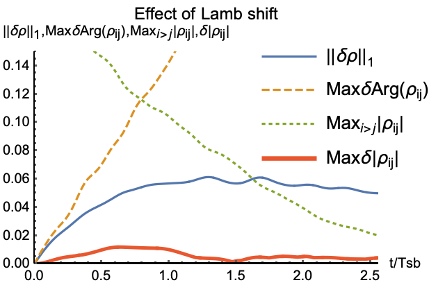
Refer to caption
Figure 7: Thin: the error ‖ρC​(t)−ρC​L​(t)‖1\|\rho_{C}(t)-\rho_{CL}(t)\|_{1} of dropping the Lamb shift HL​SH_{LS} for Ta,adjT_{a,\text{adj}}. Thick: the maximum difference in the magnitude of the matrix elements maxi​j⁡δ​|ρC,i​j|\max_{ij}\delta|\rho_{C,ij}|. Dashed: the maximum difference in the phase of the matrix elements. Dotted: the decay of the off-diagonal matrix elements.

6 Error bounds and estimates

In this section we give the details of the various error bounds and estimates mentioned without proof in our derivation of the CGME in Sec. 3. Our strategy is to derive the error terms successively, and then add them up using the triangle inequality. We work our way up through the various approximations, starting from Born in Sec. 6.2, followed by Markov in Sec. 6.3, then time-averaging (or coarse-graining) in Sec. 6.4. In the course of the latter, we bound the error due to dropping part of the integration domain to achieve complete positivity, and analyze the optimization of TaT_{a}. But we start with a proof of Lemma 1, which plays a central role in our analysis.

6.1 Bound on the difference of solutions of differential equations differing by a bounded operator

We first present a proof of Lemma 1.

Proof.

The first part of the Lemma is concerned with the pair of differential equations x˙=ℒt​x+ℰ\dot{x}=\mathcal{L}_{t}x+\mathcal{E} and y˙=ℒt​y\dot{y}=\mathcal{L}_{t}y. Their formal solution is:

x⁡(t)=x⁡(0)+∫0tℒτ​(x⁡(τ))​𝑑τ+∫0tℰ​𝑑τ,y⁡(t)=y⁡(0)+∫0tℒτ​(y⁡(τ))​𝑑τ.x(t)=x(0)+\int_{0}^{t}\mathcal{L}_{\tau}(x(\tau))d\tau+\int_{0}^{t}\mathcal{E}d\tau,\quad y(t)=y(0)+\int_{0}^{t}\mathcal{L}_{\tau}(y(\tau))d\tau\ . (142)

Let Λ>0\Lambda>0 be a constant defined as follows: supτ,x‖ℒτ​(x)‖1≤Λ\sup_{\tau,x}\|\mathcal{L}_{\tau}(x)\|_{1}\leq\Lambda for all xx such that ‖x‖1=1\|x\|_{1}=1. Since ℒ\mathcal{L} is linear, and writing x=δ/‖δ‖1x=\delta/\|\delta\|_{1}, it follows that ∀δ\forall\delta: ‖ℒτ​(δ)‖1=‖δ‖1​‖ℒτ​(x)‖1≤‖δ‖1​Λ\|\mathcal{L}_{\tau}(\delta)\|_{1}=\|\delta\|_{1}\|\mathcal{L}_{\tau}(x)\|_{1}\leq\|\delta\|_{1}\Lambda. Then, assuming x⁡(0)=y⁡(0)x(0)=y(0), and taking the operator norm of the difference yields, for δ=x⁡(t)−y⁡(t)\delta=x(t)-y(t):

‖x⁡(t)−y⁡(t)‖1≤Λ​∫0t‖x⁡(τ)−y⁡(τ)‖1​𝑑τ+t​‖ℰ‖1,\|x(t)-y(t)\|_{1}\leq\Lambda\int_{0}^{t}\|x(\tau)-y(\tau)\|_{1}d\tau+t\|\mathcal{E}\|_{1}\ , (143)

Many different functions f⁡(t)≡‖x⁡(t)−y⁡(t)‖1f(t)\equiv\|x(t)-y(t)\|_{1} satisfy this inequality for all tt, but they are all upper-bounded by the function b1​(t)=max⁡‖x⁡(t)−y⁡(t)‖1b_{1}(t)=\max\|x(t)-y(t)\|_{1} that saturates the inequality:

b˙1=Λ​b1+‖ℰ‖1,b1​(0)=0.\dot{b}_{1}=\Lambda b_{1}+\|\mathcal{E}\|_{1},\quad b_{1}(0)=0\ . (144)

The solution is

b1​(t)\displaystyle b_{1}(t) =(eΛ​t−1)​‖ℰ‖1Λ\displaystyle=(e^{\Lambda t}-1)\frac{\|\mathcal{E}\|_{1}}{\Lambda} (145a)
≤(ec−1)​‖ℰ‖1Λ∀t≤cΛ.\displaystyle\leq(e^{c}-1)\frac{\|\mathcal{E}\|_{1}}{\Lambda}\quad\forall t\leq\frac{c}{\Lambda}\ . (145b)

This proves the desired bound on ‖x⁡(t)−y⁡(t)‖1≤b1​(t)\|x(t)-y(t)\|_{1}\leq b_{1}(t).

The second part of the Lemma is concerned with the more general, non-Markovian pair of differential equations x˙​(t)=∫0tKt−τ​(x⁡(τ))​𝑑τ+ℰ\dot{x}(t)=\int_{0}^{t}K_{t-\tau}(x(\tau))d\tau+\mathcal{E} and y˙​(t)=∫0tKt−τ​(y⁡(τ))​𝑑τ\dot{y}(t)=\int_{0}^{t}K_{t-\tau}(y(\tau))d\tau. The first part of the Lemma in fact follows from this case as a corollary, but we presented it for clarity. We again subtract the formal solutions:

x⁡(t)−y⁡(t)=∫0t∫0τKτ−θ​(x⁡(θ)−y⁡(θ))​𝑑τ​𝑑θ+∫0tℰ​𝑑τ.x(t)-y(t)=\int_{0}^{t}\int_{0}^{\tau}K_{\tau-\theta}(x(\theta)-y(\theta))d\tau d\theta+\int_{0}^{t}\mathcal{E}d\tau\ . (146)

Define Λt=supx‖Kt​(x)‖1\Lambda_{t}=\sup_{x}\|K_{t}(x)\|_{1} for all xx such that ‖x‖1=1\|x\|_{1}=1. By linearity of KtK_{t} it follows as above that ∀δ\forall\delta: ‖Kt​(δ)‖1≤Λt​‖δ‖1\|K_{t}(\delta)\|_{1}\leq\Lambda_{t}\|\delta\|_{1}. Therefore:

‖x⁡(t)−y⁡(t)‖1≤∫0t∫0τΛτ−θ​‖x⁡(θ)−y⁡(θ)‖1​𝑑τ​𝑑θ+∫0t‖ℰ‖1​𝑑τ.\|x(t)-y(t)\|_{1}\leq\int_{0}^{t}\int_{0}^{\tau}\Lambda_{\tau-\theta}\|x(\theta)-y(\theta)\|_{1}d\tau d\theta+\int_{0}^{t}\|\mathcal{E}\|_{1}d\tau\ . (147)

The upper bound bK​(t)b_{K}(t) on ‖x⁡(t)−y⁡(t)‖1\|x(t)-y(t)\|_{1} satisfies the equation:

bK​(t)=∫0t∫0τΛτ−θ​bK​(θ)​𝑑τ​𝑑θ+‖ℰ‖1​t.b_{K}(t)=\int_{0}^{t}\int_{0}^{\tau}\Lambda_{\tau-\theta}b_{K}(\theta)d\tau d\theta+\|\mathcal{E}\|_{1}t\ . (148)

Taking the derivative once, we obtain:

b˙K​(t)=∫0tΛt−τ​bK​(τ)​𝑑τ+‖ℰ‖1.\dot{b}_{K}(t)=\int_{0}^{t}\Lambda_{t-\tau}b_{K}(\tau)d\tau+\|\mathcal{E}\|_{1}\ . (149)

Since the r.h.s. is positive, bK​(t)b_{K}(t) is a monotonic function. So bK​(τ)≤bK​(t)b_{K}(\tau)\leq b_{K}(t), and it follows that:

b˙K​(t)≤∫0tΛt−τ​bK​(t)​𝑑τ+‖ℰ‖1.\dot{b}_{K}(t)\leq\int_{0}^{t}\Lambda_{t-\tau}b_{K}(t)d\tau+\|\mathcal{E}\|_{1}\ . (150)

In other words, we can again upper-bound bK​(t)≤bK′​(t)b_{K}(t)\leq b_{K}^{\prime}(t), such that

b˙K′​(t)=∫0tΛt−τ​𝑑τ​bK′​(t)+‖ℰ‖1.\dot{b}_{K}^{\prime}(t)=\int_{0}^{t}\Lambda_{t-\tau}d\tau b_{K}^{\prime}(t)+\|\mathcal{E}\|_{1}\ . (151)

Now let Λ\Lambda be a positive constant such that ∫0tΛτ​𝑑τ≤Λ\int_{0}^{t}\Lambda_{\tau}d\tau\leq\Lambda for all tt. We thus arrive at

bK˙′′​(t)=Λ​bK′′​(t)+‖ℰ‖1,\dot{b_{K}}^{\prime\prime}(t)=\Lambda b_{K}^{\prime\prime}(t)+\|\mathcal{E}\|_{1}\ , (152)

for a new upper-bound bK′′​(t)≥bK′​(t)b_{K}^{\prime\prime}(t)\geq b_{K}^{\prime}(t). This is exactly the same as Eq. (144), and hence the Lemma still holds for non-Markovian equations. ∎

Note that for our purposes Λ=4/τS​B\Lambda=4/\tau_{SB} is usually taken, thanks to Eq. (41, 42c), and that the non-Markovian bound will be generalized in Sec. 6.2. The exponential on the r.h.s. of Eq. (145b) may be troublesome. Under additional assumptions we can prove a much tighter linear in tt bound presented in Appendix E, yet we did not find a way to recast all of our results in that tighter form.

6.2 Born approximation error

We start with an estimate of the error associated with making the Born approximation, which we presented as the estimate ‖ℰB‖1=O⁡(τBτS​B2)\|\mathcal{E}_{B}\|_{1}=O\left(\frac{\tau_{B}}{\tau_{SB}^{2}}\right) in Eq. (33). I.e., we would like to bound the error ℰB=ρ˙true,I​(t)−∫0tKt−τ2,B​(ρtrue,I​(τ))​𝑑τ\mathcal{E}_{B}=\dot{\rho}_{\text{true},I}(t)-\int_{0}^{t}K_{t-\tau}^{2,B}(\rho_{\text{true},I}(\tau))d\tau. It is difficult to do so directly since ρtrue,I​(t)\rho_{\text{true},I}(t) is unknown, so instead we will first use a proxy for ρtrue,I​(t)\rho_{\text{true},I}(t), which we call ρB​4,I​(t)\rho_{B4,I}(t). The latter is the solution of the master equation obtained by iterating the substitution of ρtot=ρtot​(0)−i​∫0t[V⁡(τ),ρtot​(τ)]​𝑑τ\rho_{\text{tot}}=\rho_{\text{tot}}(0)-i\int_{0}^{t}[V(\tau),\rho_{\text{tot}}(\tau)]d\tau [Eq. (29b)] into ρ˙tot​(t)=−i⁡[V⁡(t),ρtot​(t)]{\dot{\rho}}_{\text{tot}}(t)=-i[V(t),\rho_{\text{tot}}(t)] [Eq. (29a)] to 4th order, and only then applying the Born approximation. After developing an understanding of the 4th order we proceed to the infinite series. We make certain assumptions about its convergence, and comment below on their compatibility with the known convergence radius of the Dyson series. Let us first define the type of bath for which we can carry out this procedure in order to arrive at a bound.

We refer to a bath as exponential if its correlation function 𝒞⁡(t)\mathcal{C}(t) decays exponentially. This type of assumption is both common and convenient. For example, as we will see in more detail below, for a Gaussian bath (one which satisfies Wick’s theorem) the times t1<t2<t3<t4t_{1}<t_{2}<t_{3}<t_{4} appear in the estimate of the Born error [they enter terms such as 𝒞⁡(t1−t3)​𝒞​(t2−t4)\mathcal{C}(t_{1}-t_{3})\mathcal{C}(t_{2}-t_{4})]. If 𝒞⁡(t)\mathcal{C}(t) is exponentially decaying with a characteristic time τB\tau_{B}, that immediately lets us conclude that only t1,t2,t3,t4t_{1},t_{2},t_{3},t_{4} that are all within ∼τB\sim\tau_{B} of each other contribute to the estimate, and the bound on the Born error acquires a small factor of τB/τS​B\tau_{B}/\tau_{SB}. However, an exponentially decaying 𝒞⁡(t)\mathcal{C}(t) may be an unrealistically strong assumption (e.g., it is hard to satisfy at low temperatures). Therefore it is desirable to introduce a condition weaker than exponential decay, which we refer to as a non-exponential bath. Specifically, we consider the convergence of integrals such as ∫0∞|𝒞⁡(t)|​tn​𝑑t\int_{0}^{\infty}|\mathcal{C}(t)|t^{n}dt for some integer n≥0n\geq 0. Such a condition was used in Ref. [31] to control the error of the subsequent Markov approximation. Here we show how these integrals for n=0,1n=0,1 control our estimate of the Born error for a Gaussian bath. The physical meaning of these integrals was defined in Eq. (11). A more general requirement on a non-Gaussian bath can be derived in the same way. However, that requirement will involve a higher-order correlation function that does not have a straightforward and concise interpretation.

Recall the steps of the derivation where we make the Born approximation, leading to Eq. (39). For brevity, we drop the interaction picture subscript, replace the time argument by a subscript, and place the approximation level BB in the superscript: ρB,I​(t)=ρtB\rho_{B,I}(t)=\rho_{t}^{B}. Written out explicitly, Eq. (39) in terms of ρtB\rho_{t}^{B} is:

ρ˙tB=∫0tKt−τ2,B​(ρτB)​𝑑τ=∫0t𝒞⁡(τ−t)​(At​ρτB​Aτ−ρτB​Aτ​At)+𝒞⁡(t−τ)​(Aτ​ρτB​At−At​Aτ​ρτB)​𝑑τ.{\dot{\rho}}^{B}_{t}=\int_{0}^{t}K_{t-\tau}^{2,B}(\rho_{\tau}^{B})d\tau=\int_{0}^{t}\mathcal{C}(\tau-t)(A_{t}\rho^{B}_{\tau}A_{\tau}-\rho^{B}_{\tau}A_{\tau}A_{t})+\mathcal{C}(t-\tau)(A_{\tau}\rho^{B}_{\tau}A_{t}-A_{t}A_{\tau}\rho^{B}_{\tau})d\tau\ . (153)

The formal solution is:

ρτB=ρ0+∫0τd​θ​∫0θd​m​𝒞​(m−θ)​(Aθ​ρmB​Am−ρmB​Am​Aθ)+𝒞⁡(θ−m)​(Am​ρmB​Aθ−Aθ​Am​ρmB).{\rho}^{B}_{\tau}=\rho_{0}+\int_{0}^{\tau}d\theta\int_{0}^{\theta}dm\mathcal{C}(m-\theta)(A_{\theta}\rho^{B}_{m}A_{m}-\rho^{B}_{m}A_{m}A_{\theta})+\mathcal{C}(\theta-m)(A_{m}\rho^{B}_{m}A_{\theta}-A_{\theta}A_{m}\rho^{B}_{m}). (154)

We substitute this solution back into Eq. (153), a necessary step because our estimate of the Born error will come from the 4th order terms, so we need to subtract the original solution. The full expression to be subtracted is:

ρ˙tB\displaystyle{\dot{\rho}}^{B}_{t} =∫0tKt−τ2,B​(∫0τ∫0θKθ−m2,B​(ρmB)​𝑑m​𝑑θ)​𝑑τ=∫0tKt−m4,B​(ρmB)​𝑑τ\displaystyle=\int_{0}^{t}K_{t-\tau}^{2,B}\left(\int_{0}^{\tau}\int_{0}^{\theta}K_{\theta-m}^{2,B}(\rho_{m}^{B})dmd\theta\right)d\tau=\int_{0}^{t}K_{t-m}^{4,B}(\rho_{m}^{B})d\tau (155a)
=∫0t𝒞⁡(τ−t)​(At​ρ0​Aτ−ρ0​Aτ​At)+𝒞⁡(t−τ)​(Aτ​ρ0​At−At​Aτ​ρ0)​𝑑τ\displaystyle=\int_{0}^{t}\mathcal{C}(\tau-t)(A_{t}\rho_{0}A_{\tau}-\rho_{0}A_{\tau}A_{t})+\mathcal{C}(t-\tau)(A_{\tau}\rho_{0}A_{t}-A_{t}A_{\tau}\rho_{0})d\tau (155b)
+∫0tdτ∫0τdθ∫0θdm\displaystyle+\int_{0}^{t}d\tau\int_{0}^{\tau}d\theta\int_{0}^{\theta}dm (155c)
[\displaystyle[ 𝒞⁡(τ−t)​𝒞​(m−θ)​At​(Aθ​ρmB​Am−ρmB​Am​Aθ)​Aτ+𝒞⁡(τ−t)​𝒞​(θ−m)​At​(Am​ρmB​Aθ−Aθ​Am​ρmB)​Aτ\displaystyle\mathcal{C}(\tau-t)\mathcal{C}(m-\theta)A_{t}(A_{\theta}\rho^{B}_{m}A_{m}-\rho^{B}_{m}A_{m}A_{\theta})A_{\tau}+\mathcal{C}(\tau-t)\mathcal{C}(\theta-m)A_{t}(A_{m}\rho^{B}_{m}A_{\theta}-A_{\theta}A_{m}\rho^{B}_{m})A_{\tau} (155d)
−\displaystyle- 𝒞⁡(τ−t)​𝒞​(m−θ)​(Aθ​ρmB​Am−ρmB​Am​Aθ)​Aτ​At−𝒞⁡(τ−t)​𝒞​(θ−m)​(Am​ρmB​Aθ−Aθ​Am​ρmB)​Aτ​At\displaystyle\mathcal{C}(\tau-t)\mathcal{C}(m-\theta)(A_{\theta}\rho^{B}_{m}A_{m}-\rho^{B}_{m}A_{m}A_{\theta})A_{\tau}A_{t}-\mathcal{C}(\tau-t)\mathcal{C}(\theta-m)(A_{m}\rho^{B}_{m}A_{\theta}-A_{\theta}A_{m}\rho^{B}_{m})A_{\tau}A_{t} (155e)
+\displaystyle+ 𝒞⁡(t−τ)​𝒞​(m−θ)​Aτ​(Aθ​ρmB​Am−ρmB​Am​Aθ)​At+𝒞⁡(t−τ)​𝒞​(θ−m)​Aτ​(Am​ρmB​Aθ−Aθ​Am​ρmB)​At\displaystyle\mathcal{C}(t-\tau)\mathcal{C}(m-\theta)A_{\tau}(A_{\theta}\rho^{B}_{m}A_{m}-\rho^{B}_{m}A_{m}A_{\theta})A_{t}+\mathcal{C}(t-\tau)\mathcal{C}(\theta-m)A_{\tau}(A_{m}\rho^{B}_{m}A_{\theta}-A_{\theta}A_{m}\rho^{B}_{m})A_{t} (155f)
−\displaystyle- 𝒞(t−τ)𝒞(m−θ)AtAτ(AθρmBAm−ρmBAmAθ)−𝒞(t−τ)𝒞(θ−m)AtAτ(AmρmBAθ−AθAmρmB)].\displaystyle\mathcal{C}(t-\tau)\mathcal{C}(m-\theta)A_{t}A_{\tau}(A_{\theta}\rho^{B}_{m}A_{m}-\rho^{B}_{m}A_{m}A_{\theta})-\mathcal{C}(t-\tau)\mathcal{C}(\theta-m)A_{t}A_{\tau}(A_{m}\rho^{B}_{m}A_{\theta}-A_{\theta}A_{m}\rho^{B}_{m})]\ . (155g)

Now, these terms constitute only a part of the expression for the derivative of the true density matrix ρ˙ttrue{\dot{\rho}}^{\text{true}}_{t} to the 44th order in the system-bath interaction. The full 44th order expression can be obtained, as mentioned above, by substituting the solution of the total evolution, ρtot=ρtot​(0)−i​∫0t[V⁡(τ),ρtot​(τ)]​𝑑τ\rho_{\text{tot}}=\rho_{\text{tot}}(0)-i\int_{0}^{t}[V(\tau),\rho_{\text{tot}}(\tau)]d\tau into ρ˙tot​(t)=−i⁡[V⁡(t),ρtot​(t)]{\dot{\rho}}_{\text{tot}}(t)=-i[V(t),\rho_{\text{tot}}(t)] three consecutive times (to generate a 4th order commutator), and only then applying the Born approximation. We call this ρtB​4\rho_{t}^{B4} since it will differ from ρtB\rho_{t}^{B} in the 4th order in the interaction V⁡(t)V(t). Doing so, we obtain:

ρ˙tB​4\displaystyle{\dot{\rho}}^{B4}_{t} =∫0t𝒞⁡(τ−t)​(At​ρ0​Aτ−ρ0​Aτ​At)+𝒞⁡(t−τ)​(Aτ​ρ0​At−At​Aτ​ρ0)​𝑑τ\displaystyle=\int_{0}^{t}\mathcal{C}(\tau-t)(A_{t}\rho_{0}A_{\tau}-\rho_{0}A_{\tau}A_{t})+\mathcal{C}(t-\tau)(A_{\tau}\rho_{0}A_{t}-A_{t}A_{\tau}\rho_{0})d\tau (156a)
+Trb​[At⊗Bt,∫0td​τ​[Aτ⊗Bτ,∫0τd​θ​[Aθ⊗Bθ,∫0θd​m​[Am⊗Bm,ρmB​4⊗ρb]]]].\displaystyle+\mathrm{Tr}_{\text{b}}[A_{t}\otimes B_{t},\int_{0}^{t}d\tau[A_{\tau}\otimes B_{\tau},\int_{0}^{\tau}d\theta[A_{\theta}\otimes B_{\theta},\int_{0}^{\theta}dm[A_{m}\otimes B_{m},\rho^{B4}_{m}\otimes\rho_{\text{b}}]]]]\ . (156b)

Defined in this way, ρtB​4{\rho}^{B4}_{t} is close to the 44th order of the true state ρttrue{\rho}^{\text{true}}_{t} up to terms of 66th order and higher, so we use ρtB​4−ρtB\rho^{B4}_{t}-\rho^{B}_{t} to estimate the actual leading order error ρttrue−ρtB\rho^{\text{true}}_{t}-\rho^{B}_{t}. We proceed to expand all the commutators:

ρ˙tB​4=∫0tKt−τ4,B​4​(ρτB​4)​𝑑τ=∫0tKt−τ2,B​(ρ0)​𝑑τ\displaystyle{\dot{\rho}}^{B4}_{t}=\int_{0}^{t}K_{t-\tau}^{4,B4}(\rho_{\tau}^{B4})d\tau=\int_{0}^{t}K_{t-\tau}^{2,B}(\rho_{0})d\tau (157a)
+∫0tdτ∫0τdθ∫0θdmTrbBtBτBθBmρbAtAτAθAmρB​4m−TrbBtBτBθρbBmAtAτAθρB​4mAm−…\displaystyle+\int_{0}^{t}d\tau\int_{0}^{\tau}d\theta\int_{0}^{\theta}dm\mathrm{Tr}_{\text{b}}B_{t}B_{\tau}B_{\theta}B_{m}\rho_{\text{b}}A_{t}A_{\tau}A_{\theta}A_{m}\rho^{B4}_{m}-\mathrm{Tr}_{\text{b}}B_{t}B_{\tau}B_{\theta}\rho_{\text{b}}B_{m}A_{t}A_{\tau}A_{\theta}\rho^{B4}_{m}A_{m}-\dots (157b)

There are 16 terms total in the last line, and the order of Bt,Bτ,Bθ,BmB_{t},B_{\tau},B_{\theta},B_{m} and ρb\rho_{\text{b}} is exactly the same as the order of At,Aτ,Aθ,AmA_{t},A_{\tau},A_{\theta},A_{m} and ρmB\rho^{B}_{m}.

Let us now assume that the bath is Gaussian. By definition, a Gaussian bath obeys Wick’s theorem (or Isserlis’ theorem [75]), which states that at all orders the higher order correlation functions decouple into products of two-point correlation functions. For example, for the 4-point correlation function:

Trb​Bt​Bτ​Bθ​Bm​ρb=Trb​Bt​Bτ​ρb​Trb​Bθ​Bm​ρb+Trb​Bt​Bθ​ρb​Trb​Bτ​Bm​ρb+Trb​Bt​Bm​ρb​Trb​Bτ​Bθ​ρb.\mathrm{Tr}_{\text{b}}B_{t}B_{\tau}B_{\theta}B_{m}\rho_{\text{b}}=\mathrm{Tr}_{\text{b}}B_{t}B_{\tau}\rho_{\text{b}}\mathrm{Tr}_{\text{b}}B_{\theta}B_{m}\rho_{\text{b}}+\mathrm{Tr}_{\text{b}}B_{t}B_{\theta}\rho_{\text{b}}\mathrm{Tr}_{\text{b}}B_{\tau}B_{m}\rho_{\text{b}}+\mathrm{Tr}_{\text{b}}B_{t}B_{m}\rho_{\text{b}}\mathrm{Tr}_{\text{b}}B_{\tau}B_{\theta}\rho_{\text{b}}\ . (158)

By definition, 𝒞⁡(t−τ)=Trb​Bt​Bτ​ρb\mathcal{C}(t-\tau)=\mathrm{Tr}_{\text{b}}B_{t}B_{\tau}\rho_{\text{b}}. Thus:

Trb​Bt​Bτ​Bθ​Bm​ρb=𝒞⁡(t−τ)​𝒞​(θ−m)+𝒞⁡(t−θ)​𝒞​(τ−m)+𝒞⁡(t−m)​𝒞​(τ−θ)\mathrm{Tr}_{\text{b}}B_{t}B_{\tau}B_{\theta}B_{m}\rho_{\text{b}}=\mathcal{C}(t-\tau)\mathcal{C}(\theta-m)+\mathcal{C}(t-\theta)\mathcal{C}(\tau-m)+\mathcal{C}(t-m)\mathcal{C}(\tau-\theta) (159)

We see that in Eq. (155) only the first term was present. One can check that the order of AA is exactly the same, so upon subtracting Eq. (155) from Eq. (158) only the two terms 𝒞⁡(t−θ)​𝒞​(τ−m)+𝒞⁡(t−m)​𝒞​(τ−θ)\mathcal{C}(t-\theta)\mathcal{C}(\tau-m)+\mathcal{C}(t-m)\mathcal{C}(\tau-\theta) remain. These extra terms can be interpreted in terms of the corresponding diagrammatic technique. Indeed, note that t>τ>θ>mt>\tau>\theta>m. If in Wick’s theorem we have a pairing t↔τ,θ↔mt\leftrightarrow\tau,\penalty\ \theta\leftrightarrow m and the arrows are drawn above the time axis, they do not relate to each other, and each arc can be anywhere along the time axis. But if the pairing is t↔θ,τ↔mt\leftrightarrow\theta,\penalty\ \tau\leftrightarrow m or t↔m,τ↔θt\leftrightarrow m,\penalty\ \tau\leftrightarrow\theta, then the two arcs are stuck together due to the condition t>τ>θ>mt>\tau>\theta>m; see Fig. 8.

Refer to caption
Figure 8: Different possible pairings of Trb​Bt​Bτ​Bθ​Bm​ρb\mathrm{Tr}_{\text{b}}B_{t}B_{\tau}B_{\theta}B_{m}\rho_{\text{b}} in Wick’s theorem. Note that the first and second order are in τB/τS​B\tau_{B}/\tau_{SB}, not in the coupling strength itself, in which both diagrams are 4th order.

At the moment we have two equations: the Born equation in two forms Eq. (153) and Eq. (155), as well as the 4th order equation Eq. (157a):

ρ˙tB=∫0tKt−τ2,B​(ρτB)​𝑑τ=∫0tKt−τ4,B​(ρτB)​𝑑τ,ρ˙tB​4=∫0tKt−τ4,B​4​(ρτB​4)​𝑑τ,{\dot{\rho}}^{B}_{t}=\int_{0}^{t}K_{t-\tau}^{2,B}(\rho_{\tau}^{B})d\tau=\int_{0}^{t}K_{t-\tau}^{4,B}(\rho_{\tau}^{B})d\tau,\quad{\dot{\rho}}^{B4}_{t}=\int_{0}^{t}K_{t-\tau}^{4,B4}(\rho_{\tau}^{B4})d\tau, (160)

where K⁡(ρ)K(\rho) are corresponding linear superoperators. K2,BK^{2,B} is the 2nd order (in the bath interaction) operator from Eq. (153), K4,BK^{4,B} and K4,B​4K^{4,B4} have terms up to the 4th order defined in Eq. (155) and Eq. (157a). Define

ℰB​4​(ρany)\displaystyle\mathcal{E}_{B4}(\rho^{\text{any}}) =∫0t(Kt−τ4,B​4​(ρτany)−Kt−τ4,B​(ρτany))​𝑑τ,\displaystyle=\int_{0}^{t}(K_{t-\tau}^{4,B4}(\rho_{\tau}^{\text{any}})-K_{t-\tau}^{4,B}(\rho_{\tau}^{\text{any}}))d\tau\ , (161)

for instance:

ℰB​4​(ρB4)=ρ˙tB​4−∫0tKt−τ4,B​(ρτB​4)​𝑑τ.\mathcal{E}_{B4}(\rho^{\text{B4}})={\dot{\rho}}^{B4}_{t}-\int_{0}^{t}K_{t-\tau}^{4,B}(\rho_{\tau}^{B4})d\tau\ . (162)

Define

ℰB\displaystyle\mathcal{E}_{B} =ρ˙ttrue−∫0tKt−τ2,B​(ρτtrue)​𝑑τ.\displaystyle={\dot{\rho}}^{\text{true}}_{t}-\int_{0}^{t}K_{t-\tau}^{2,B}(\rho_{\tau}^{\text{true}})d\tau\ . (163)

The quantity that appeared in the derivation is ℰB\mathcal{E}_{B}. We will now bound ‖ℰB​4​(ρany)‖1\|\mathcal{E}_{B4}(\rho^{\text{any}})\|_{1} and discuss its generalization ‖ℰB​k​(ρany)‖1\|\mathcal{E}_{Bk}(\rho^{\text{any}})\|_{1}. We postpone the estimate for ‖ℰB‖1\|\mathcal{E}_{B}\|_{1} till we develop more advanced tools.

The difference Kt−τ4,B​4​(ρτ4,B​4)−Kt−τ4,B​(ρτB​4)K_{t-\tau}^{4,B4}(\rho_{\tau}^{4,B4})-K_{t-\tau}^{4,B}(\rho_{\tau}^{B4}) is given by the two second order pairings in Fig. 8, times the 1616 possible orders of At,Aτ,Aθ,AmA_{t},A_{\tau},A_{\theta},A_{m} and ρm\rho_{m}:

ℰB​4=∫0td​τ​∫0τd​θ​∫0θd​m​(𝒞⁡(t−θ)​𝒞​(τ−m)+𝒞⁡(t−m)​𝒞​(τ−θ))​At​Aτ​Aθ​Am​ρmany−…\mathcal{E}_{B4}=\int_{0}^{t}d\tau\int_{0}^{\tau}d\theta\int_{0}^{\theta}dm(\mathcal{C}(t-\theta)\mathcal{C}(\tau-m)+\mathcal{C}(t-m)\mathcal{C}(\tau-\theta))A_{t}A_{\tau}A_{\theta}A_{m}\rho^{\text{any}}_{m}-\dots (164)

We take the trace norm of both sides:

‖ℰB​4​(ρany)‖1≤∫0td​τ​∫0τd​θ​∫0θd​m​‖(𝒞⁡(t−θ)​𝒞​(τ−m)+𝒞⁡(t−m)​𝒞​(τ−θ))​At​Aτ​Aθ​Am​ρmany‖1+…\|\mathcal{E}_{B4}(\rho^{\text{any}})\|_{1}\leq\int_{0}^{t}d\tau\int_{0}^{\tau}d\theta\int_{0}^{\theta}dm\|(\mathcal{C}(t-\theta)\mathcal{C}(\tau-m)+\mathcal{C}(t-m)\mathcal{C}(\tau-\theta))A_{t}A_{\tau}A_{\theta}A_{m}\rho^{\text{any}}_{m}\|_{1}+\dots (165)

where we used the triangle inequality ‖A+B‖1≤‖A‖1+‖B‖1\|A+B\|_{1}\leq\|A\|_{1}+\|B\|_{1}. We now use submultiplicativity [Eq. (38)]. Noting that the first norm in the submultiplicativity inequality is the operator norm, we obtain:

‖ℰB​4​(ρany)‖1≤∫0td​τ​∫0τd​θ​∫0θd​m​‖(𝒞⁡(t−θ)​𝒞​(τ−m)+𝒞⁡(t−m)​𝒞​(τ−θ))​At​Aτ​Aθ​Am‖​‖ρmany‖1+…\|\mathcal{E}_{B4}(\rho^{\text{any}})\|_{1}\leq\int_{0}^{t}d\tau\int_{0}^{\tau}d\theta\int_{0}^{\theta}dm\|(\mathcal{C}(t-\theta)\mathcal{C}(\tau-m)+\mathcal{C}(t-m)\mathcal{C}(\tau-\theta))A_{t}A_{\tau}A_{\theta}A_{m}\|\|\rho^{\text{any}}_{m}\|_{1}+\dots (166)

The operator norm ‖A‖=1\|A\|=1 and we will set ca=maxt​‖ρtany‖1c_{a}=\text{max}_{t}\|\rho^{\text{any}}_{t}\|_{1} such that ‖ρany‖1≤ca\|\rho^{\text{any}}\|_{1}\leq c_{a}:

‖ℰB​4​(ρany)‖1≤ca​∫0td​τ​∫0τd​θ​∫0θd​m​|(𝒞⁡(t−θ)​𝒞​(τ−m)+𝒞⁡(t−m)​𝒞​(τ−θ))|+…\|\mathcal{E}_{B4}(\rho^{\text{any}})\|_{1}\leq c_{a}\int_{0}^{t}d\tau\int_{0}^{\tau}d\theta\int_{0}^{\theta}dm|(\mathcal{C}(t-\theta)\mathcal{C}(\tau-m)+\mathcal{C}(t-m)\mathcal{C}(\tau-\theta))|+\dots (167)

In particular, ℰB​4​(ρB)\mathcal{E}_{B4}(\rho^{B}) is bounded with cBc_{B} and ℰB​4​(ρB​4)\mathcal{E}_{B4}(\rho^{B4}) with cB​4c_{B4}. There are 1616 terms after the expansion of commutators:

‖ℰB​4​(ρany)‖≤16​ca​∫0td​τ​∫0τd​θ​∫0θd​m​|𝒞⁡(t−θ)||𝒞⁡(τ−m)|+|𝒞⁡(t−m)|​|𝒞⁡(τ−θ)|,\|\mathcal{E}_{B4}(\rho^{\text{any}})\|\leq 16c_{a}\int_{0}^{t}d\tau\int_{0}^{\tau}d\theta\int_{0}^{\theta}dm|\mathcal{C}(t-\theta)||\mathcal{C}(\tau-m)|+|\mathcal{C}(t-m)||\mathcal{C}(\tau-\theta)|\ , (168)

where we have also used that |𝒞⁡(t−m)|=|𝒞​(m−t)∗|=|𝒞⁡(m−t)||\mathcal{C}(t-m)|=|\mathcal{C}(m-t)^{*}|=|\mathcal{C}(m-t)|. What is left is to bound the integrals in Eq. (164). It turns out that the following condition suffices:

∫0∞|𝒞⁡(t)|​tn​𝑑t≤τBnτS​B,for n=0,1,\int_{0}^{\infty}|\mathcal{C}(t)|t^{n}dt\leq\frac{\tau_{B}^{n}}{\tau_{SB}}\ ,\quad\text{for $n=0,1$}\ , (169)

which is automatically satisfied for τS​B\tau_{SB} and τB\tau_{B} as defined in Eq. (11). We also change the order of integration variables using the condition 0≤m≤θ≤τ≤t0\leq m\leq\theta\leq\tau\leq t, e.g.:

∫0td​τ​∫0τ𝑑θ=∫0td​θ​∫θt𝑑τ.\int_{0}^{t}d\tau\int_{0}^{\tau}d\theta=\int_{0}^{t}d\theta\int_{\theta}^{t}d\tau. (170)

The first term in Eq. (164) is bounded as:

∫0td​τ​∫0τd​θ​[∫0θd​m​|𝒞⁡(τ−m)|]​|𝒞⁡(t−θ)|\displaystyle\int_{0}^{t}d\tau\int_{0}^{\tau}d\theta\left[\int_{0}^{\theta}dm|\mathcal{C}(\tau-m)|\right]|\mathcal{C}(t-\theta)| ≤1τS​B​∫0td​τ​∫0τ𝑑θ|𝒞⁡(t−θ)|=1τS​B​∫0td​θ​∫θtd​τ​|𝒞⁡(t−θ)|\displaystyle\leq\frac{1}{\tau_{SB}}\int_{0}^{t}d\tau\int_{0}^{\tau}d\theta|\mathcal{C}(t-\theta)|=\frac{1}{\tau_{SB}}\int_{0}^{t}d\theta\int_{\theta}^{t}d\tau|\mathcal{C}(t-\theta)| (171a)
=1τS​B​∫0t(t−θ)​𝑑θ​|𝒞⁡(t−θ)|≤τBτS​B2,\displaystyle=\frac{1}{\tau_{SB}}\int_{0}^{t}(t-\theta)d\theta|\mathcal{C}(t-\theta)|\leq\frac{\tau_{B}}{\tau_{SB}^{2}}, (171b)

while the second term in Eq. (164) is bounded as:

∫0td​τ​∫0τd​θ​∫0θd​m​|𝒞⁡(t−m)|​|𝒞⁡(τ−θ)|\displaystyle\int_{0}^{t}d\tau\int_{0}^{\tau}d\theta\int_{0}^{\theta}dm|\mathcal{C}(t-m)||\mathcal{C}(\tau-\theta)| =∫0td​m​∫mtd​θ​[∫θtd​τ​|𝒞⁡(τ−θ)|]​|𝒞⁡(t−m)|\displaystyle=\int_{0}^{t}dm\int_{m}^{t}d\theta\left[\int_{\theta}^{t}d\tau|\mathcal{C}(\tau-\theta)|\right]|\mathcal{C}(t-m)| (172a)
≤1τS​B​∫0td​m​∫mt𝑑θ|𝒞⁡(t−m)|=1τS​B​∫0t(t−m)​𝑑m​|𝒞⁡(t−m)|\displaystyle\leq\frac{1}{\tau_{SB}}\int_{0}^{t}dm\int_{m}^{t}d\theta|\mathcal{C}(t-m)|=\frac{1}{\tau_{SB}}\int_{0}^{t}(t-m)dm|\mathcal{C}(t-m)| (172b)
≤τBτS​B2.\displaystyle\leq\frac{\tau_{B}}{\tau_{SB}^{2}}\ . (172c)

Together, this yields:

‖ℰB​4​(ρany)‖1≤32​ca​τBτS​B2,\|\mathcal{E}_{B4}(\rho^{\text{any}})\|_{1}\leq 32c_{a}\frac{\tau_{B}}{\tau_{SB}^{2}}\ , (173)

which is the first hint for the result given in Eq. (33). The actual error term appearing in Eq. (32) is ℰB\mathcal{E}_{B} as defined in Eq. (163). We can consider repeating the construction of ρB​4\rho^{B4} presented here for ρB​6,ρB​8​…\rho^{B6},\rho^{B8}\dots as successive approximations to ρtrue\rho^{\text{true}}. The corresponding errors can be defined:

ℰB​k​(ρany)=∫0t(Kt−τk,B​k​(ρτany)−Kt−τk,B​(ρτany))​𝑑τ,\mathcal{E}_{Bk}(\rho^{\text{any}})=\int_{0}^{t}(K_{t-\tau}^{k,Bk}(\rho_{\tau}^{\text{any}})-K_{t-\tau}^{k,B}(\rho_{\tau}^{\text{any}}))d\tau\ , (174)

By employing the diagrammatic technique as in Fig. 8, the higher orders of perturbation theory in the system-bath coupling can be shown to give higher orders in τB/τS​B\tau_{B}/\tau_{SB}. There are also extra factors of 4​t/τS​B4t/\tau_{SB} that appear in the higher orders. For instance, ℰB​6\mathcal{E}_{B6} has the form:

‖ℰB​6​(ρany)‖1≤32​ca​τBτS​B2​(1+8​tτS​B+O⁡(τBτS​B)),\|\mathcal{E}_{B6}(\rho^{\text{any}})\|_{1}\leq 32c_{a}\frac{\tau_{B}}{\tau_{SB}^{2}}\left(1+\frac{8t}{\tau_{SB}}+O\left(\frac{\tau_{B}}{\tau_{SB}}\right)\right), (175)

and the diagrams for the second term are shown in Fig. 9(a). We do not prove this form of ℰB​6\mathcal{E}_{B6} here. We will bound all tt-dependent terms of the first order in τB/τS​B\tau_{B}/\tau_{SB}, by summing the diagrams in Fig. 9(b):

Refer to caption
Figure 9: Diagrams contributing to the second order of (a) ℰB​6\mathcal{E}_{B6}, (b) ℰB​k\mathcal{E}_{Bk} for arbitrary kk.
‖ℰB​k​(ρany)‖1\displaystyle\|\mathcal{E}_{Bk}(\rho^{\text{any}})\|_{1} ≤32​ca​τBτS​B2​(∑m=1k/2−1m(m−1)!​(4​tτS​B)m−1+O⁡(τBτS​B))\displaystyle\leq 32c_{a}\frac{\tau_{B}}{\tau_{SB}^{2}}\left(\sum_{m=1}^{k/2-1}\frac{m}{(m-1)!}\left(\frac{4t}{\tau_{SB}}\right)^{m-1}+O\left(\frac{\tau_{B}}{\tau_{SB}}\right)\right) (176a)
≤32​ca​τBτS​B2​((1+4​t/τS​B)​e4​t/τS​B+O⁡(τBτS​B)),\displaystyle\leq 32c_{a}\frac{\tau_{B}}{\tau_{SB}^{2}}\left((1+4t/\tau_{SB})e^{4t/\tau_{SB}}+O\left(\frac{\tau_{B}}{\tau_{SB}}\right)\right)\ , (176b)

for all kk. Here we fix time to be a constant: ∃ϵ⁡(t),C⁡(t)\exists\epsilon(t),C(t) s.t. O⁡(τBτS​B)≤C⁡(t)​τBτS​BO\left(\frac{\tau_{B}}{\tau_{SB}}\right)\leq C(t)\frac{\tau_{B}}{\tau_{SB}} for all τBτS​B≤ϵ⁡(t)\frac{\tau_{B}}{\tau_{SB}}\leq\epsilon(t). This is a weak statement. A stronger statement would include the time-dependence inside big-OO, and have time-independent constants ϵ,C\epsilon,C:

‖ℰB​k​(ρany)‖1≤32​ca​e4​t/τS​B​τBτS​B2​(1+4​t/τS​B+O⁡(e4​t/τS​B​τB/τS​B))\|\mathcal{E}_{Bk}(\rho^{\text{any}})\|_{1}\leq 32c_{a}e^{4t/\tau_{SB}}\frac{\tau_{B}}{\tau_{SB}^{2}}(1+4t/\tau_{SB}+O(e^{4t/\tau_{SB}}\tau_{B}/\tau_{SB})) (177)

We do not know how to prove such a statement as of yet. The proof would rely on the diagrammatic calculation of subleading terms. It is straightforward, but cumbersome, and we do not attempt it here. Instead we make two assumptions:

  1. 1.

    In the k→∞k\to\infty limit, there is a finite radius of convergence in e4​t/τS​B​τB/τS​Be^{4t/\tau_{SB}}\tau_{B}/\tau_{SB}:

    ‖ℰB​∞​(ρany)‖1≤32​ca​e4​t/τS​B​τBτS​B2​(1+4​t/τS​B+O⁡(e4​t/τS​B​τB/τS​B)).\|\mathcal{E}_{B\infty}(\rho^{\text{any}})\|_{1}\leq 32c_{a}e^{4t/\tau_{SB}}\frac{\tau_{B}}{\tau_{SB}^{2}}(1+4t/\tau_{SB}+O(e^{4t/\tau_{SB}}\tau_{B}/\tau_{SB}))\ . (178)
  2. 2.

    The true solution is the limit of the perturbative series:

    ρ˙ttrue=∫0tKt−τ∞,B​∞​(ρτtrue)​𝑑τ.{\dot{\rho}}^{\text{true}}_{t}=\int_{0}^{t}K_{t-\tau}^{\infty,B\infty}(\rho_{\tau}^{\text{true}})d\tau\ . (179)

To prove convergence, one needs to control the factorial number of terms appearing in Wick’s theorem. Such a proof was already presented by Davies [4]. The slight adjustments needed to include an integral condition such as Eq. (169) are a somewhat tedious problem left for a future study.

Our definition of ℰB\mathcal{E}_{B} under this assumption contains ℰB​∞\mathcal{E}_{B\infty} discussed above, as well as an extra term:

ℰB\displaystyle\mathcal{E}_{B} =ρ˙ttrue−∫0tKt−τ2,B​(ρτtrue)​𝑑τ=∫0t(Kt−τ∞,B​∞​(ρτtrue)−Kt−τ2,B​(ρτtrue))​𝑑τ\displaystyle={\dot{\rho}}^{\text{true}}_{t}-\int_{0}^{t}K_{t-\tau}^{2,B}(\rho_{\tau}^{\text{true}})d\tau=\int_{0}^{t}(K_{t-\tau}^{\infty,B\infty}(\rho_{\tau}^{\text{true}})-K_{t-\tau}^{2,B}(\rho_{\tau}^{\text{true}}))d\tau (180a)
‖ℰB‖1\displaystyle\|\mathcal{E}_{B}\|_{1} ≤‖∫0t(Kt−τ∞,B​∞​(ρτtrue)−Kt−τ∞,B​(ρτtrue))​𝑑τ‖1+‖∫0t(Kt−τ∞,B​(ρτtrue)−Kt−τ2,B​(ρτtrue))​𝑑τ‖1\displaystyle\leq\left\|\int_{0}^{t}(K_{t-\tau}^{\infty,B\infty}(\rho_{\tau}^{\text{true}})-K_{t-\tau}^{\infty,B}(\rho_{\tau}^{\text{true}}))d\tau\right\|_{1}+\left\|\int_{0}^{t}(K_{t-\tau}^{\infty,B}(\rho_{\tau}^{\text{true}})-K_{t-\tau}^{2,B}(\rho_{\tau}^{\text{true}}))d\tau\right\|_{1} (180b)
≤32​τBτS​B2​(1+O⁡(τB/τS​B))+‖∫0t(Kt−τ∞,B​(ρτtrue)−Kt−τ2,B​(ρτtrue))​𝑑τ‖1,\displaystyle\leq 32\frac{\tau_{B}}{\tau_{SB}^{2}}(1+O(\tau_{B}/\tau_{SB}))+\left\|\int_{0}^{t}(K_{t-\tau}^{\infty,B}(\rho_{\tau}^{\text{true}})-K_{t-\tau}^{2,B}(\rho_{\tau}^{\text{true}}))d\tau\right\|_{1}\ , (180c)

where ca=1c_{a}=1 since the true evolution is CP. The second term will turn out to be time-dependent, and quite tricky to estimate. We will return to this problem after we develop some extra machinery.

Let us first note the form of Kk,BK^{k,B}, starting with k=4k=4:

∫0tKt−τ4,B​(ρτany)​𝑑τ=∫0tKt−τ2,B​(ρ0+∫0τ∫0mKm−θ2,B​(ρmany)​𝑑m​𝑑θ)​𝑑τ.\int_{0}^{t}K^{4,B}_{t-\tau}(\rho^{\text{any}}_{\tau})d\tau=\int_{0}^{t}K^{2,B}_{t-\tau}\left(\rho_{0}+\int_{0}^{\tau}\int_{0}^{m}K^{2,B}_{m-\theta}(\rho^{\text{any}}_{m})dmd\theta\right)d\tau\ . (181)

The solution of

ρ˙B​4=∫0tKt−τ4,B​4​(ρτB​4)​𝑑τ=∫0tKt−τ4,B​(ρτB​4)​𝑑τ+ℰB​4\dot{\rho}^{B4}=\int_{0}^{t}K^{4,B4}_{t-\tau}(\rho_{\tau}^{B4})d\tau=\int_{0}^{t}K^{4,B}_{t-\tau}(\rho^{B4}_{\tau})d\tau+\mathcal{E}_{B4} (182)

is equivalent to solving a system of 44th order equations that are our proxy for the true solution (which is ∞\infty order):

{ρ˙B​4=∫0tKt−τ2,B​(ρτ(1))​dτ+ℰB​4,ρB​4​(0)=ρ0ρ˙(1)=∫0tKt−τ2,B​(ρτB​4)​dτ,ρ(1)​(0)=ρ0.\left\{\begin{array}[]{ll}\dot{\rho}^{B4}=\int_{0}^{t}K^{2,B}_{t-\tau}(\rho^{(1)}_{\tau})d\tau+\mathcal{E}_{B4},&\rho^{B4}(0)=\rho_{0}\\ \dot{\rho}^{(1)}=\int_{0}^{t}K^{2,B}_{t-\tau}(\rho^{B4}_{\tau})d\tau,&\rho^{(1)}(0)=\rho_{0}\ .\end{array}\right. (183)

We will prove that the solution of the above system remains close to ρB\rho^{B}, the solution of the equation after the Born approximation:

ρ˙B=∫0tKt−τ2,B​(ρτB)​𝑑τ.\dot{\rho}^{B}=\int_{0}^{t}K^{2,B}_{t-\tau}(\rho^{B}_{\tau})d\tau\ . (184)

We will also present a straightforward generalization to all kk which will allow one to bound ‖ℰB‖1\|\mathcal{E}_{B}\|_{1}.

First write the equation in the compact form:

𝐩˙=𝐋𝐩+𝐄,𝐩=()ρ(𝟏)ρ𝐁𝟒,𝐋=()∫𝐊𝐭−τ​𝐝τ 0𝟎∫𝐊𝐭−τ​𝐝τ,𝐄=()𝟎ℰ𝐁𝟒​(ρ𝐁𝟒).\dot{\bf{p}}=\bf{Lp}+\bf{E},\hskip 11.49994pt\bf{p}=\left(\penalty\ {}^{\rho^{B4}}_{\rho^{(1)}}\right),\hskip 11.49994pt\bf{L}=\left(\penalty\ {}^{0\penalty\ \hskip 9.06108pt\hskip 9.06108pt\penalty\ \int K_{t-\tau}d\tau}_{\int K_{t-\tau}d\tau\penalty\ \hskip 9.06108pt\hskip 9.06108pt\penalty\ 0}\right),\hskip 11.49994pt\bf{E}=\left(\penalty\ {}^{\mathcal{E}_{B4}(\rho^{B4})}_{0}\right)\ . (185)

Define a custom norm that is an infinity norm on the vector of operators, but for each operator the trace norm is taken:

∥𝐯∥c=‖‖v2v1c=max(∥v1∥1,∥v2∥1)\|{\bf{v}}\|_{c}=\left\|\penalty\ {}^{v^{1}}_{v^{2}}\right\|_{c}=\text{max}(\|v^{1}\|_{1},\|v^{2}\|_{1}) (186)

The triangle inequality is obeyed as required:

‖𝐯+𝐰‖c\displaystyle\|{\bf{v}+\bf{w}}\|_{c} =max​(‖v1+w1‖1,‖v2+w2‖1)≤max​(‖v1‖1+‖w1‖1,‖v2‖1+‖w2‖1)\displaystyle=\text{max}(\|v^{1}+w^{1}\|_{1},\|v^{2}+w^{2}\|_{1})\leq\text{max}(\|v^{1}\|_{1}+\|w^{1}\|_{1},\|v^{2}\|_{1}+\|w^{2}\|_{1}) (187a)
≤max​(‖v1‖1,‖v2‖1)+max​(‖w1‖1,‖w2‖1)=‖𝐯‖c+‖𝐰‖c.\displaystyle\leq\text{max}(\|v^{1}\|_{1},\|v^{2}\|_{1})+\text{max}(\|w^{1}\|_{1},\|w^{2}\|_{1})=\|{\bf{v}}\|_{c}+\|{\bf{w}}\|_{c}\ . (187b)

The maximum of the custom norm of 𝐋{\bf{L}} over inputs of norm 1 is the same as before:

max𝐩:‖𝐩‖c=1∥𝐋𝐩∥c=Λ=4τS​B,\text{max}_{{\bf{p}}:\|{\bf{p}}\|_{c}=1}\|{\bf{Lp}}\|_{c}=\Lambda=\frac{4}{\tau_{SB}}\ , (188)

so all the properties needed to prove Lemma 1 hold. We establish:

‖δ​𝐩t‖c≤eΛ​t−1Λ​‖𝐄‖c\|\delta{\bf{p}}_{t}\|_{c}\leq\frac{e^{\Lambda t}-1}{\Lambda}\|{\bf{E}}\|_{c} (189)

in the original variables:

max​(‖δ​ρt(1)‖1,‖δ​ρtB​4‖1)≤eΛ​t−1Λ​‖ℰB​4‖1.\text{max}(\|\delta\rho^{(1)}_{t}\|_{1},\|\delta\rho^{B4}_{t}\|_{1})\leq\frac{e^{\Lambda t}-1}{\Lambda}\|\mathcal{E}_{B4}\|_{1}\ . (190)

Note that the error we are trying to bound is

∥ℰB∥1=‖ρ˙true−∫0tKt−τ2,B(ρτtrue)dτ‖1=‖∫0t(Kt−τ∞,B​∞(ρτtrue)−Kt−τ2,B(ρτtrue)dτ‖1.\|\mathcal{E}_{B}\|_{1}=\left\|\dot{\rho}^{\text{true}}-\int_{0}^{t}K^{2,B}_{t-\tau}(\rho^{\text{true}}_{\tau})d\tau\right\|_{1}=\left\|\int_{0}^{t}\left(K^{\infty,B\infty}_{t-\tau}(\rho^{\text{true}}_{\tau})-K^{2,B}_{t-\tau}(\rho^{\text{true}}_{\tau}\right)d\tau\right\|_{1}\ . (191)

Our approximation to it is bounded as:

‖ρ˙B​4−∫0tKt−τ2,B​(ρτB​4)​𝑑τ‖1≤‖∫0tKt−τ2,B​(ρτ(1)−ρτB​4)​𝑑τ‖1+‖ℰB​4‖1≤(2​eΛ​t−1)​‖ℰB​4‖1,\left\|\dot{\rho}^{B4}-\int_{0}^{t}K^{2,B}_{t-\tau}(\rho^{B4}_{\tau})d\tau\right\|_{1}\leq\left\|\int_{0}^{t}K^{2,B}_{t-\tau}(\rho^{(1)}_{\tau}-\rho^{B4}_{\tau})d\tau\right\|_{1}+\|\mathcal{E}_{B4}\|_{1}\leq(2e^{\Lambda t}-1)\|\mathcal{E}_{B4}\|_{1}\ , (192)

where we have used the triangle inequality: ‖ρτ(1)−ρτB​4‖1≤‖δ​ρτ(1)‖1+‖δ​ρτB​4‖1\|\rho^{(1)}_{\tau}-\rho^{B4}_{\tau}\|_{1}\leq\|\delta\rho^{(1)}_{\tau}\|_{1}+\|\delta\rho^{B4}_{\tau}\|_{1}. Now we can repeat the above proof for arbitrary kk:

{ρ˙B​k=∫0tKt−τ2,B​(ρτ(1))​dτ+ℰB​k​(ρB​k)ρB​k​(0)=ρ0ρ˙(1)=∫0tKt−τ2,B​(ρτ(2))​𝑑τρ(1)​(0)=ρ0……ρ˙(k/2−1)=∫0tKt−τ2,B​(ρτB​4)​𝑑τρ(k/2−1)​(0)=ρ0\left\{\begin{array}[]{ll}\dot{\rho}^{Bk}=\int_{0}^{t}K^{2,B}_{t-\tau}(\rho^{(1)}_{\tau})d\tau+\mathcal{E}_{Bk}(\rho^{Bk})&\rho^{Bk}(0)=\rho_{0}\\ \dot{\rho}^{(1)}=\int_{0}^{t}K^{2,B}_{t-\tau}(\rho^{(2)}_{\tau})d\tau&\rho^{(1)}(0)=\rho_{0}\\ \dots&\dots\\ \dot{\rho}^{(k/2-1)}=\int_{0}^{t}K^{2,B}_{t-\tau}(\rho^{B4}_{\tau})d\tau&\rho^{(k/2-1)}(0)=\rho_{0}\end{array}\right. (193)

For appropriately defined 𝐋{\bf{L}}, ∥⋅∥c\|\cdot\|_{c} the r.h.s. is still bounded by the same constant:

max𝐩:‖𝐩‖c=1∥𝐋𝐩∥c=Λ=4τS​B,\text{max}_{{\bf{p}}:\|{\bf{p}}\|_{c}=1}\|{\bf{Lp}}\|_{c}=\Lambda=\frac{4}{\tau_{SB}}\ , (194)

which leads to

max​(‖δ​ρt(1)‖1,…,‖δ​ρtB​k‖1)≤eΛ​t−1Λ​‖ℰB​k‖1,\text{max}(\|\delta\rho^{(1)}_{t}\|_{1},\dots,\|\delta\rho^{Bk}_{t}\|_{1})\leq\frac{e^{\Lambda t}-1}{\Lambda}\|\mathcal{E}_{Bk}\|_{1}\ , (195)

and the error in the r.h.s. is bounded without change:

‖ρ˙B​k−∫0tKt−τ2,B​(ρτB​k)​𝑑τ‖1≤‖∫0tKt−τ2,B​(ρτ(1)−ρτB​k)​𝑑τ‖1+‖ℰB​k‖1≤(2​eΛ​t−1)​‖ℰB​k‖1.\left\|\dot{\rho}^{Bk}-\int_{0}^{t}K^{2,B}_{t-\tau}(\rho^{Bk}_{\tau})d\tau\right\|_{1}\leq\left\|\int_{0}^{t}K^{2,B}_{t-\tau}(\rho^{(1)}_{\tau}-\rho^{Bk}_{\tau})d\tau\right\|_{1}+\|\mathcal{E}_{Bk}\|_{1}\leq(2e^{\Lambda t}-1)\|\mathcal{E}_{Bk}\|_{1}\ . (196)

Taking the k→∞k\to\infty limit, we obtain:

‖ρttrue−ρtB‖1≤eΛ​t−1Λ​‖ℰB​∞​(ρtrue)‖1≤8​(e4​t/τS​B−1)​e4​t/τS​B​τBτS​B​(1+4​t/τS​B+O⁡(e4​t/τS​B​τB/τS​B)),\|\rho^{\text{true}}_{t}-\rho^{B}_{t}\|_{1}\leq\frac{e^{\Lambda t}-1}{\Lambda}\|\mathcal{E}_{B\infty}(\rho^{\text{true}})\|_{1}\leq 8(e^{4t/\tau_{SB}}-1)e^{4t/\tau_{SB}}\frac{\tau_{B}}{\tau_{SB}}(1+4t/\tau_{SB}+O(e^{4t/\tau_{SB}}\tau_{B}/\tau_{SB}))\ , (197)

and, finally:

‖ℰB‖1\displaystyle\|\mathcal{E}_{B}\|_{1} ≤(2​eΛ​t−1)​‖ℰB​∞​(ρtrue)‖1\displaystyle\leq(2e^{\Lambda t}-1)\|\mathcal{E}_{B\infty}(\rho^{\text{true}})\|_{1} (198a)
≤32​(2​e4​t/τS​B−1)​e4​t/τS​B​τBτS​B2​(1+4​t/τS​B+O⁡(e4​t/τS​B​τB/τS​B)),\displaystyle\leq 32(2e^{4t/\tau_{SB}}-1)e^{4t/\tau_{SB}}\frac{\tau_{B}}{\tau_{SB}^{2}}(1+4t/\tau_{SB}+O(e^{4t/\tau_{SB}}\tau_{B}/\tau_{SB}))\ , (198b)

where we have used that ca=1c_{a}=1 for ρtrue\rho^{\text{true}}. This result is the sought-after justification of the estimate ‖ℰB‖1=O⁡(τBτS​B2)\|\mathcal{E}_{B}\|_{1}=O\left(\frac{\tau_{B}}{\tau_{SB}^{2}}\right) given in Eq. (33).

An immediate consequence of Eq. (197) is that we can use it to obtain a bound on cBc_{B}, which we defined after Eq. (40) as an upper bound on ‖ρB,I‖1\|\rho_{B,I}\|_{1}. Since

‖ρtB‖1≤‖ρttrue‖1+‖ρtB−ρttrue‖1=1+‖ρttrue−ρtB‖1,\|\rho^{B}_{t}\|_{1}\leq\|\rho^{\text{true}}_{t}\|_{1}+\|\rho^{B}_{t}-\rho^{\text{true}}_{t}\|_{1}=1+\|\rho^{\text{true}}_{t}-\rho^{B}_{t}\|_{1}\ , (199)

we obtain:

cB≤1+8​(e4​t/τS​B−1)​e4​t/τS​B​τBτS​B​(1+4​t/τS​B+O⁡(e4​t/τS​B​τB/τS​B)).c_{B}\leq 1+8(e^{4t/\tau_{SB}}-1)e^{4t/\tau_{SB}}\frac{\tau_{B}}{\tau_{SB}}(1+4t/\tau_{SB}+O(e^{4t/\tau_{SB}}\tau_{B}/\tau_{SB}))\ . (200)

6.3 Markov approximation error

This subsection follows Ref. [76] initially. Before the Markov approximation but after the Born approximation, the master equation had the form given in Eq. (39). The error due the Markov approximation ρB,I​(τ)↦ρB,I​(t)\rho_{B,I}(\tau)\mapsto\rho_{B,I}(t), in transitioning to Eq. (42b), is:

ℰM=∫0t𝒞⁡(τ−t)​[A⁡(t)​(ρB,I​(τ)−ρB,I​(t))​A​(τ)−(ρB,I​(τ)−ρB,I​(t))​A​(τ)​A​(t)]​𝑑τ+h.c.\mathcal{E}_{M}=\int_{0}^{t}\mathcal{C}(\tau-t)[A(t)(\rho_{B,I}(\tau)-\rho_{B,I}(t))A(\tau)-(\rho_{B,I}(\tau)-\rho_{B,I}(t))A(\tau)A(t)]d\tau+\textrm{h.c.} (201)

Since ρB,I​(t)−ρB,I​(τ)=∫τtρ˙B,I​(t′)​d​t′\rho_{B,I}(t)-\rho_{B,I}(\tau)=\int_{\tau}^{t}{\dot{\rho}}_{B,I}(t^{\prime})dt^{\prime}, we have

‖ρB,I​(t)−ρB,I​(τ)‖1≤‖ρ˙B,I‖1​(t−τ)≤4​(t−τ)​cBτS​B,\|\rho_{B,I}(t)-\rho_{B,I}(\tau)\|_{1}\leq\|{\dot{\rho}}_{B,I}\|_{1}(t-\tau)\leq\frac{4(t-\tau)c_{B}}{\tau_{SB}}\ , (202)

where we used Eq. (40) in the second inequality. Now we can estimate the norm of the error:

‖ℰM‖1≤4​∫0t|𝒞⁡(τ−t)|​4​(t−τ)τS​B​𝑑τ≤16​τB​cBτS​B2.\|\mathcal{E}_{M}\|_{1}\leq 4\int_{0}^{t}|\mathcal{C}(\tau-t)|\frac{4(t-\tau)}{\tau_{SB}}d\tau\leq 16\frac{\tau_{B}c_{B}}{\tau_{SB}^{2}}\ . (203)

We found cBc_{B} and saw that it is O⁡(1)O(1) in Eq. (200).

Let us now use the Markovian Lemma 1 with Eq. (203):

‖ρtB​M−ρtB‖1≤4​τB​cBτS​B​(e4​t/τS​B−1).\|\rho^{BM}_{t}-\rho^{B}_{t}\|_{1}\leq 4\frac{\tau_{B}c_{B}}{\tau_{SB}}\left(e^{4t/\tau_{SB}}-1\right)\ . (204)

A total expression for the Born and Markov error is [adding Eq. (197)]:

‖ρttrue−ρtB​M‖1≤4​τB​cBτS​B​(e4​t/τS​B−1)+8​(e4​t/τS​B−1)​e4​t/τS​B​τBτS​B​(1+4​t/τS​B+O⁡(e4​t/τS​B​τB/τS​B)),\|\rho^{\text{true}}_{t}-\rho^{BM}_{t}\|_{1}\leq 4\frac{\tau_{B}c_{B}}{\tau_{SB}}\left(e^{4t/\tau_{SB}}-1\right)+8(e^{4t/\tau_{SB}}-1)e^{4t/\tau_{SB}}\frac{\tau_{B}}{\tau_{SB}}(1+4t/\tau_{SB}+O(e^{4t/\tau_{SB}}\tau_{B}/\tau_{SB}))\ , (205)

which simplifies to:

‖ρttrue−ρtB​M‖1≤4​(e4​t/τS​B−1)​τBτS​B​(cB+2​e4​t/τS​B​(1+4​t/τS​B+O⁡(e4​t/τS​B​τB/τS​B))),\|\rho^{\text{true}}_{t}-\rho^{BM}_{t}\|_{1}\leq 4(e^{4t/\tau_{SB}}-1)\frac{\tau_{B}}{\tau_{SB}}\left(c_{B}+2e^{4t/\tau_{SB}}(1+4t/\tau_{SB}+O(e^{4t/\tau_{SB}}\tau_{B}/\tau_{SB}))\right)\ , (206)

or substituting in cBc_{B}:

‖ρttrue−ρtB​M‖1≤(e4​tτS​B−1)​τB​(4+8​(1+4​(e4​tτS​B−1)​τBτS​B)​e4​tτS​B​(1+4​tτS​B+O⁡(e4​tτS​B​τBτS​B)))τS​B.\|\rho^{\text{true}}_{t}-\rho^{BM}_{t}\|_{1}\leq\frac{\left(e^{\frac{4t}{\tau_{SB}}}-1\right)\tau_{B}\left(4+8\left(1+\frac{4\left(e^{\frac{4t}{\tau_{SB}}}-1\right)\tau_{B}}{\tau_{SB}}\right)e^{\frac{4t}{\tau_{SB}}}\left(1+\frac{4t}{\tau_{SB}}+O\left(e^{\frac{4t}{\tau_{SB}}}\frac{\tau_{B}}{\tau_{SB}}\right)\right)\right)}{\tau_{SB}}\ . (207)

The extra factor from cBc_{B} can be absorbed into the big-OO notation:

‖ρttrue−ρtB​M‖1≤(e4​tτS​B−1)​τB​(4+8​e4​tτS​B​(1+4​tτS​B)​(1+O⁡(e4​tτS​B​τBτS​B)))τS​B.\|\rho^{\text{true}}_{t}-\rho^{BM}_{t}\|_{1}\leq\frac{\left(e^{\frac{4t}{\tau_{SB}}}-1\right)\tau_{B}\left(4+8e^{\frac{4t}{\tau_{SB}}}\left(1+\frac{4t}{\tau_{SB}}\right)\left(1+O\left(e^{\frac{4t}{\tau_{SB}}}\frac{\tau_{B}}{\tau_{SB}}\right)\right)\right)}{\tau_{SB}}\ . (208)

A loose bound follows from the above:

‖ρttrue−ρtB​M‖1≤12​(e4​tτS​B−1)​e8​tτS​B​τB​(1+O⁡(e4​tτS​B​τBτS​B))τS​B.\|\rho^{\text{true}}_{t}-\rho^{BM}_{t}\|_{1}\leq\frac{12\left(e^{\frac{4t}{\tau_{SB}}}-1\right)e^{\frac{8t}{\tau_{SB}}}\tau_{B}\left(1+O\left(e^{\frac{4t}{\tau_{SB}}}\frac{\tau_{B}}{\tau_{SB}}\right)\right)}{\tau_{SB}}\ . (209)

Sometimes we wish to report the bound briefly as:

‖ρttrue−ρtB​M‖1=(e4​tτS​B−1)​O​(e8​tτS​B​τBτS​B)\|\rho^{\text{true}}_{t}-\rho^{BM}_{t}\|_{1}=\left(e^{\frac{4t}{\tau_{SB}}}-1\right)O\left(e^{\frac{8t}{\tau_{SB}}}\frac{\tau_{B}}{\tau_{SB}}\right) (210)
Proof.

The original big-O notation states that for e4​tτS​B​τBτS​B≤ϵe^{\frac{4t}{\tau_{SB}}}\frac{\tau_{B}}{\tau_{SB}}\leq\epsilon the following inequality holds:

‖ρttrue−ρtB​M‖1≤12​(e4​tτS​B−1)​e8​tτS​B​τB​(1+C​e4​tτS​B​τBτS​B)τS​B≤12​(e4​tτS​B−1)​e8​tτS​B​τB​(1+C​ϵ)τS​B.\|\rho^{\text{true}}_{t}-\rho^{BM}_{t}\|_{1}\leq\frac{12\left(e^{\frac{4t}{\tau_{SB}}}-1\right)e^{\frac{8t}{\tau_{SB}}}\tau_{B}\left(1+Ce^{\frac{4t}{\tau_{SB}}}\frac{\tau_{B}}{\tau_{SB}}\right)}{\tau_{SB}}\leq\frac{12\left(e^{\frac{4t}{\tau_{SB}}}-1\right)e^{\frac{8t}{\tau_{SB}}}\tau_{B}\left(1+C\epsilon\right)}{\tau_{SB}}\ . (211)

We first note that e4​tτS​B≤e8​tτS​Be^{\frac{4t}{\tau_{SB}}}\leq e^{\frac{8t}{\tau_{SB}}}, so if e8​tτS​B​τBτS​B≤ϵe^{\frac{8t}{\tau_{SB}}}\frac{\tau_{B}}{\tau_{SB}}\leq\epsilon, then e4​tτS​B​τBτS​B≤ϵe^{\frac{4t}{\tau_{SB}}}\frac{\tau_{B}}{\tau_{SB}}\leq\epsilon as well, and we are within the range of the original big-O notation. By taking 12​(1+C​ϵ)12(1+C\epsilon) as the new constant, we prove Eq. (210). ∎

6.4 Time averaging error and its optimization

6.4.1 General analysis of time-averaging

We consider the time-averaging operation, which leads to a more complicated bound on the difference of the solutions. We first prove a general result:

Lemma 2.

For any first order linear differential equation ρ˙​(t)=ℒt​ρ​(t)\dot{\rho}(t)=\mathcal{L}_{t}\rho(t) there is a time-averaged version

π˙(t)=ℒt¯π(t),ℒt¯=1Ta∫−Ta/2Ta/2ℒt+τdτ.\dot{\pi}(t)=\overline{\mathcal{L}_{t}}\pi(t),\quad\overline{\mathcal{L}_{t}}=\frac{1}{T_{a}}\int_{-T_{a}/2}^{T_{a}/2}\mathcal{L}_{t+\tau}d\tau\ . (212)

Note that we use a different symbol π⁡(t)\pi(t) for the solution of the time-averaged equation. Assume the same initial condition: ρ⁡(0)=π⁡(0)\rho(0)=\pi(0). Then the deviation between the two, δ​ρ​(t)≡π⁡(t)−ρ⁡(t)\delta\rho(t)\equiv\pi(t)-\rho(t), is bounded as:

‖δ​ρ​(t)‖1≤[b2​(min⁡(t,Ta/2))+cρ​Λ​Ta/4]​max⁡(eΛ⁡(t−Ta/2),1)−cρ​Λ​Ta/4,\displaystyle\|\delta\rho(t)\|_{1}\leq[b_{2}(\min(t,T_{a}/2))+c_{\rho}\Lambda T_{a}/4]\max(e^{\Lambda(t-T_{a}/2)},1)-c_{\rho}\Lambda T_{a}/4\ , (213)

where Λ,cρ\Lambda,c_{\rho} are constants such that ∀t,ρ0,‖ρ0‖1≤1:‖ℒt​(ρ0)‖1≤Λ\forall t,\rho_{0},\|\rho_{0}\|_{1}\leq 1:\penalty\ \|\mathcal{L}_{t}(\rho_{0})\|_{1}\leq\Lambda and the solution ρ⁡(t)\rho(t) with the initial condition ρ⁡(0)=ρ0\rho(0)=\rho_{0} is bounded as ‖ρ⁡(t)‖1≤cρ\|\rho(t)\|_{1}\leq c_{\rho}. The function b2​(t)b_{2}(t) is:

b2​(t)≡4​cρ​tTa+cρ​4−2​Λ​Ta−(Λ​Ta/2)2Λ​Ta​(1−eΛ​t).b_{2}(t)\equiv 4c_{\rho}\frac{t}{T_{a}}+c_{\rho}\frac{4-2\Lambda T_{a}-(\Lambda T_{a}/2)^{2}}{\Lambda T_{a}}(1-e^{\Lambda t})\ . (214)

An immediate corollary is:

‖δ​ρ​(t)‖1=O⁡(Λ​Ta)​ for ​t=O⁡(Λ−1).\|\delta\rho(t)\|_{1}=O(\Lambda T_{a})\text{ for }t=O(\Lambda^{-1})\ . (215)

The proof can be found in Appendix F. The O⁡(Λ​Ta)O(\Lambda T_{a}) corollary enters the estimate for ‖ρB​M,I​(t)−ρB​M​T,I​(t)‖1\|\rho_{BM,I}(t)-\rho_{BMT,I}(t)\|_{1} we presented in Eq. (61b) in the derivation (using Λ=4/τS​B\Lambda=4/\tau_{SB}). We will also need a compact bound on:

b2​(Ta/2)cρ=eΛ​Ta/2​(ΛTa/2)2+4(e−ΛTa/2−1+ΛTa/2)Λ​Ta−Λ​Ta4.\frac{b_{2}(T_{a}/2)}{c_{\rho}}=e^{\Lambda T_{a}/2}\frac{(\Lambda T_{a}/2)^{2}+4(e^{-\Lambda T_{a}/2}-1+\Lambda T_{a}/2)}{\Lambda T_{a}}-\frac{\Lambda T_{a}}{4}\ . (216)

One can prove that the expression in the brackets is upper-bounded by

e−ΛTa/2−1+ΛTa/2≤(ΛTa)2/8.e^{-\Lambda T_{a}/2}-1+\Lambda T_{a}/2\leq(\Lambda T_{a})^{2}/8\ . (217)

This allows us to bound

b2​(Ta/2)≤cρ​(eΛ​Ta/2​3​Λ​Ta4−Λ​Ta4).b_{2}(T_{a}/2)\leq c_{\rho}\left(e^{\Lambda T_{a}/2}\frac{3\Lambda T_{a}}{4}-\frac{\Lambda T_{a}}{4}\right)\ . (218)

Note that the function b2​(t)b_{2}(t) is monotonic: b2​(t)≤b2​(Ta/2)b_{2}(t)\leq b_{2}(T_{a}/2). One can then loosen the bound in Lemma 2:

‖δ​ρ​(t)‖1≤{cρ​(eΛ​Ta/2​3​Λ​Ta4−Λ​Ta4),t≤Ta/2cρ​(eΛ​t​3​Λ​Ta4−Λ​Ta4),t>Ta/2=cρ​(eΛ​max⁡(t,Ta/2)​3​Λ​Ta4−Λ​Ta4).\|\delta\rho(t)\|_{1}\leq\left\{\begin{array}[]{ll}\penalty\ c_{\rho}\left(e^{\Lambda T_{a}/2}\frac{3\Lambda T_{a}}{4}-\frac{\Lambda T_{a}}{4}\right),&t\leq T_{a}/2\\ \penalty\ c_{\rho}\left(e^{\Lambda t}\frac{3\Lambda T_{a}}{4}-\frac{\Lambda T_{a}}{4}\right),&t>T_{a}/2\end{array}\right.=c_{\rho}\left(e^{\Lambda\max(t,T_{a}/2)}\frac{3\Lambda T_{a}}{4}-\frac{\Lambda T_{a}}{4}\right)\ . (219)

6.4.2 Time averaging of the Redfield ME

We now focus on the specific equations of interest to us. We already established in Eq. (42c) that we can choose Λ=4/τS​B\Lambda=4/\tau_{SB} (recall that Λ\Lambda needs to upper bound the r.h.s.: maxt,ρtest,‖ρtest‖1=1⁡‖ℒtB​M,I​(ρtest)‖1≤Λ\max_{t,\rho_{\text{test}},\|\rho_{\text{test}}\|_{1}=1}\|\mathcal{L}^{BM,I}_{t}(\rho_{\text{test}})\|_{1}\leq\Lambda). The total time-averaging error (219) is now bounded as:

‖ρB​M−ρB​M​T‖1=‖δ​ρ​(t)‖1≤cB​M​(eΛ​max⁡(t,Ta/2)​3​TaτS​B−TaτS​B),\displaystyle\|\rho_{BM}-\rho_{BMT}\|_{1}=\|\delta\rho(t)\|_{1}\leq c_{BM}\left(e^{\Lambda\max(t,T_{a}/2)}\frac{3T_{a}}{\tau_{SB}}-\frac{T_{a}}{\tau_{SB}}\right)\ , (220)

We will use both the compact bound of Eq. (220), and the tightest bound available which is a repetition of Lemma 2:

‖δ​ρ​(t)‖1≤b2​(t)=[b2​(min⁡(t,Ta/2))+cB​M​Λ​Ta/4]​max⁡(eΛ⁡(t−Ta/2),1)−cB​M​Λ​Ta/4,\displaystyle\|\delta\rho(t)\|_{1}\leq b_{2}(t)=[b_{2}(\min(t,T_{a}/2))+c_{BM}\Lambda T_{a}/4]\max(e^{\Lambda(t-T_{a}/2)},1)-c_{BM}\Lambda T_{a}/4\ , (221)
b2​(t)=4​cB​M​tTa+cB​M​4−2​Λ​Ta−(Λ​Ta/2)2Λ​Ta​(1−eΛ​t),t<Ta/2.\displaystyle b_{2}(t)=4c_{BM}\frac{t}{T_{a}}+c_{BM}\frac{4-2\Lambda T_{a}-(\Lambda T_{a}/2)^{2}}{\Lambda T_{a}}(1-e^{\Lambda t}),\quad t<T_{a}/2\ . (222)

6.4.3 Bound on the error due to enforcing complete positivity

Recall that after the time-averaged equation is obtained, we need to drop an extra portion of the integral to obtain complete positivity [the transition to Eq. (65a)]. Before that, Eq. (64) was:

ρ˙B​M​T(t)=−i[H,ρB​M​T]+∑ω,ω′1Ta∫−Ta/2Ta/2dt′∫−tt′dτ′𝒞(τ′−t′)e−i⁡(ω​t′+ω′​τ′)(AωρB​M​TAω′−ρB​M​TAω′Aω)+h.c.,{\dot{\rho}}_{BMT}(t)=-i[H,\rho_{BMT}]+\sum_{\omega,\omega^{\prime}}\frac{1}{T_{a}}\int_{-T_{a}/2}^{T_{a}/2}dt^{\prime}\int_{-t}^{t^{\prime}}d\tau^{\prime}\mathcal{C}(\tau^{\prime}-t^{\prime})e^{-i(\omega t^{\prime}+\omega^{\prime}\tau^{\prime})}(A_{\omega}\rho_{BMT}A_{\omega^{\prime}}-\rho_{BMT}A_{\omega^{\prime}}A_{\omega})+\textrm{h.c.}\ , (223)

which changes into Eq. (65a) (same terms, but the portion of the integral is subtracted):

ρ˙C​(t)\displaystyle{\dot{\rho}}_{C}(t) =−i[H,ρC]+∑ω,ω′1Ta∫−Ta/2Ta/2dt′∫−tt′dτ′𝒞(τ′−t′)e−i⁡(ω​t′+ω′​τ′)(AωρCAω′−ρCAω′Aω)+h.c.−ℰp\displaystyle=-i[H,\rho_{C}]+\sum_{\omega,\omega^{\prime}}\frac{1}{T_{a}}\int_{-T_{a}/2}^{T_{a}/2}dt^{\prime}\int_{-t}^{t^{\prime}}d\tau^{\prime}\ \mathcal{C}(\tau^{\prime}-t^{\prime})e^{-i(\omega t^{\prime}+\omega^{\prime}\tau^{\prime})}(A_{\omega}\rho_{C}A_{\omega^{\prime}}-\rho_{C}A_{\omega^{\prime}}A_{\omega})+\textrm{h.c.}-\mathcal{E}_{p} (224a)
ℰp\displaystyle\mathcal{E}_{p} =∑ω,ω′1Ta∫−Ta/2Ta/2dt′∫−t−Ta/2dτ′𝒞(τ′−t′)e−i⁡(ω​t′+ω′​τ′)(AωρCAω′−ρCAω′Aω)+h.c.\displaystyle=\sum_{\omega,\omega^{\prime}}\frac{1}{T_{a}}\int_{-T_{a}/2}^{T_{a}/2}dt^{\prime}\int_{-t}^{-T_{a}/2}d\tau^{\prime}\ \mathcal{C}(\tau^{\prime}-t^{\prime})e^{-i(\omega t^{\prime}+\omega^{\prime}\tau^{\prime})}(A_{\omega}\rho_{C}A_{\omega^{\prime}}-\rho_{C}A_{\omega^{\prime}}A_{\omega})+\textrm{h.c.} (224b)

Collecting ∑ω\sum_{\omega} into A⁡(t)A(t) we obtain:

ℰp=1Ta∫−Ta/2Ta/2dt′∫−t−Ta/2dτ′𝒞(τ′−t′)(A(t′)ρCA(τ′)−ρCA(τ′)A(t′))+h.c.,\mathcal{E}_{p}=\frac{1}{T_{a}}\int_{-T_{a}/2}^{T_{a}/2}dt^{\prime}\int_{-t}^{-T_{a}/2}d\tau^{\prime}\ \mathcal{C}(\tau^{\prime}-t^{\prime})(A(t^{\prime})\rho_{C}A(\tau^{\prime})-\rho_{C}A(\tau^{\prime})A(t^{\prime}))+\textrm{h.c.}\ , (225)

so that:

∥ℰp∥1≤4Ta∫−Ta/2Ta/2dt′|∫−t−Ta/2dτ′|𝒞(τ′−t′)||.\|\mathcal{E}_{p}\|_{1}\leq\frac{4}{T_{a}}\int_{-T_{a}/2}^{T_{a}/2}dt^{\prime}\left|\int_{-t}^{-T_{a}/2}d\tau^{\prime}|\mathcal{C}(\tau^{\prime}-t^{\prime})|\right|\ . (226)
Refer to caption
Figure 10: Times contributing to ℰp\mathcal{E}_{p} for (a) t>Ta/2t>T_{a}/2 (b) t<Ta/2t<T_{a}/2

Since the resulting equation is CP, we used ‖ρC‖1=1\|\rho_{C}\|_{1}=1. We would like to bound this norm by splitting the integration domain into different times. The corresponding domains are illustrated in Fig. 10. For t<Ta/2t<T_{a}/2 we note that the argument of 𝒞⁡(τ′−t′)\mathcal{C}(\tau^{\prime}-t^{\prime}) can be both positive and negative. Thus a factor of 22 arises when we bound ∫d​t′​|𝒞⁡(τ′−t′)|≤2/τS​B\int dt^{\prime}|\mathcal{C}(\tau^{\prime}-t^{\prime})|\leq 2/\tau_{SB}:

‖ℰp‖1≤8τS​B​Ta/2−tTa≤4τS​B.\|\mathcal{E}_{p}\|_{1}\leq\frac{8}{\tau_{SB}}\frac{T_{a}/2-t}{T_{a}}\leq\frac{4}{\tau_{SB}}\ . (227)

For t>Ta/2t>T_{a}/2, we perform a change of variables: τ′−t′=−τ,t′+Ta/2=θ\tau^{\prime}-t^{\prime}=-\tau,\penalty\ t^{\prime}+T_{a}/2=\theta:

∥ℰp∥1≤4Ta∫−Ta/2−Ta/2dt′∫−t−Ta/2dτ′|𝒞(τ′−t′)|=4Ta∫0Tadθ∫θt+θ−Ta/2dτ|𝒞(τ)|.\|\mathcal{E}_{p}\|_{1}\leq\frac{4}{T_{a}}\int_{-T_{a}/2}^{-T_{a}/2}dt^{\prime}\int_{-t}^{-T_{a}/2}d\tau^{\prime}|\mathcal{C}(\tau^{\prime}-t^{\prime})|=\frac{4}{T_{a}}\int_{0}^{T_{a}}d\theta\int_{\theta}^{t+\theta-T_{a}/2}d\tau|\mathcal{C}(\tau)|\ . (228)

We now change the order of integration, noting that 0<θ<τ0<\theta<\tau, thus obtaining the following upper bound:

‖ℰp‖1≤4Ta​∫0Tad​θ​∫θt+θ−Ta/2𝑑τ|𝒞⁡(τ)|≤4Ta​∫0t+Ta/2τ​|𝒞⁡(τ)|​𝑑τ.\|\mathcal{E}_{p}\|_{1}\leq\frac{4}{T_{a}}\int_{0}^{T_{a}}d\theta\int_{\theta}^{t+\theta-T_{a}/2}d\tau|\mathcal{C}(\tau)|\leq\frac{4}{T_{a}}\int_{0}^{t+T_{a}/2}\tau|\mathcal{C}(\tau)|d\tau\ . (229)

Recall that the total evolution time TT entered the definition τBτS​B=∫0Tt​|𝒞⁡(t)|​𝑑t\frac{\tau_{B}}{\tau_{SB}}=\int_{0}^{T}t|\mathcal{C}(t)|dt [Eq. (11b)]. We can usually set T=∞T=\infty, except for an Ohmic bath [see Eq. (128)], which is a borderline applicability case, with a logarithmic in TT divergence of the integral. We define an evolution time with a collar of Ta/2T_{a}/2: T=maxt⁡(t+Ta/2)T=\max_{t}(t+T_{a}/2):

‖ℰp‖1≤4Ta​∫0Tτ​|𝒞⁡(τ)|​𝑑τ=4​τBTa​τS​B.\|\mathcal{E}_{p}\|_{1}\leq\frac{4}{T_{a}}\int_{0}^{T}\tau|\mathcal{C}(\tau)|d\tau=\frac{4\tau_{B}}{T_{a}\tau_{SB}}\ . (230)

Collecting everything, we obtain:

‖ℰp‖1​(t)≤4τS​B​(θ⁡(t−Ta/2)​τBTa+θ⁡(Ta/2−t)),\|\mathcal{E}_{p}\|_{1}(t)\leq\frac{4}{\tau_{SB}}\left(\theta(t-T_{a}/2)\frac{\tau_{B}}{T_{a}}+\theta(T_{a}/2-t)\right)\ , (231)

where θ⁡(x)=1,x>0\theta(x)=1,\penalty\ x>0 and zero otherwise.

Recall that ℰp\mathcal{E}_{p} is defined in Eq. (65a) as the extra term appearing if the CGME is written with the same expression as Eq. (64) in the r.h.s. We can now use the same idea as in the proof of Lemma 1 (Sec. 6.1). Let us introduce δ​ρ2=ρB​M​T−ρC\delta\rho_{2}=\rho_{BMT}-\rho_{C}. A function bpb_{p} that upper-bounds ‖δ​ρ2‖1\|\delta\rho_{2}\|_{1} is the solution of the differential equation

b˙p=Λ​bp+‖ℰp‖1​(t),bp​(0)=0,\dot{b}_{p}=\Lambda b_{p}+\|\mathcal{E}_{p}\|_{1}(t),\quad b_{p}(0)=0\ , (232)

where we have used Λ≥maxt,ρtest,‖ρtest‖1=1⁡‖ℒtB​M,I​(ρtest)‖1\Lambda\geq\max_{t,\rho_{\text{test}},\|\rho_{\text{test}}\|_{1}=1}\|\mathcal{L}^{BM,I}_{t}(\rho_{\text{test}})\|_{1} from Eq. (42c) as the upper bound on the norm of the superoperator on the r.h.s. of Eq. (64). Indeed, by applying the triangle inequality to the definition of the r.h.s. of Eq. (64) we get:

ℒtB​M​T,I(ρtest)=1Ta∫−Ta/2Ta/2ℒt+τB​M,I(ρtest)dτ,∥ℒtB​M​T,I(ρtest)∥1≤∥ℒtB​M,I(ρtest)∥1≤Λ.\mathcal{L}^{BMT,I}_{t}(\rho_{\text{test}})=\frac{1}{T_{a}}\int_{-T_{a}/2}^{T_{a}/2}\mathcal{L}^{BM,I}_{t+\tau}(\rho_{\text{test}})d\tau,\quad\|\mathcal{L}^{BMT,I}_{t}(\rho_{\text{test}})\|_{1}\leq\|\mathcal{L}^{BM,I}_{t}(\rho_{\text{test}})\|_{1}\leq\Lambda\ . (233)

The solution to Eq. (232) is:

bp​(t)=eΛ​t​∫0te−Λ​τ​‖ℰp‖1​(τ)​𝑑τ.b_{p}(t)=e^{\Lambda t}\int_{0}^{t}e^{-\Lambda\tau}\|\mathcal{E}_{p}\|_{1}(\tau)d\tau\ . (234)

Substituting Eq. (231), we obtain two cases:

bp​(t)\displaystyle b_{p}(t) =4Λ​τS​B​eΛ​t​(1−e−Λ​t),t<Ta/2\displaystyle=\frac{4}{\Lambda\tau_{SB}}e^{\Lambda t}\left(1-e^{-\Lambda t}\right),\quad t<T_{a}/2 (235)
bp​(t)\displaystyle b_{p}(t) =4Λ​τS​BeΛ​t((1−e−ΛTa/2)+τBTa(e−ΛTa/2−e−Λ​t)),t>Ta/2,\displaystyle=\frac{4}{\Lambda\tau_{SB}}e^{\Lambda t}\left((1-e^{-\Lambda T_{a}/2})+\frac{\tau_{B}}{T_{a}}(e^{-\Lambda T_{a}/2}-e^{-\Lambda t})\right),\quad t>T_{a}/2\ , (236)

which we can summarize as

bp​(t)≤4Λ​τS​B​[(eΛ​t−max⁡(1,eΛ⁡(t−Ta/2)))+τBTa​max⁡(eΛ⁡(t−Ta/2)−1,0)].b_{p}(t)\leq\frac{4}{\Lambda\tau_{SB}}[(e^{\Lambda t}-\max(1,e^{\Lambda(t-T_{a}/2)}))+\frac{\tau_{B}}{T_{a}}\max(e^{\Lambda(t-T_{a}/2)}-1,0)]\ . (237)

For a concise form we change the first term using 1−e−x≤x1-e^{-x}\leq x:

bp​(t)≤eΛ​t​2​TaτS​B+4​τBΛ​Ta​τS​B​max⁡(eΛ⁡(t−Ta/2)−1,0).b_{p}(t)\leq e^{\Lambda t}\frac{2T_{a}}{\tau_{SB}}+\frac{4\tau_{B}}{\Lambda T_{a}\tau_{SB}}\max(e^{\Lambda(t-T_{a}/2)}-1,0)\ . (238)

Let us now focus on the difference with ρB​M,I​(t)\rho_{BM,I}(t) which is the solution of Eq. (42b). We will keep Λ≥maxt,ρtest,‖ρtest‖1=1⁡‖ℒtB​M,I​(ρtest)‖1\Lambda\geq\max_{t,\rho_{\text{test}},\|\rho_{\text{test}}\|_{1}=1}\|\mathcal{L}^{BM,I}_{t}(\rho_{\text{test}})\|_{1} in the bound in case it is <4/τS​B<4/\tau_{SB}. Using Eqs. (220) and (238), we have:

‖ρB​M,I​(t)−ρC,I​(t)‖1≤cB​M​(eΛ​max⁡(t,Ta/2)​3​TaτS​B−TaτS​B)+eΛ​t​2​TaτS​B+4​τBΛ​Ta​τS​B​max⁡(eΛ⁡(t−Ta/2)−1,0).\displaystyle\|\rho_{BM,I}(t)-{\rho}_{C,I}(t)\|_{1}\leq c_{BM}\left(e^{\Lambda\max(t,T_{a}/2)}\frac{3T_{a}}{\tau_{SB}}-\frac{T_{a}}{\tau_{SB}}\right)+e^{\Lambda t}\frac{2T_{a}}{\tau_{SB}}+\frac{4\tau_{B}}{\Lambda T_{a}\tau_{SB}}\max(e^{\Lambda(t-T_{a}/2)}-1,0)\ . (239)

The tightest bound available that starts at zero at t=0t=0 is the combination of Eqs. (221) and (237):

‖ρB​M,I​(t)−ρC,I​(t)‖1≤[b2​(min⁡(t,Ta/2))+cB​M​Λ​Ta/4]​max⁡(eΛ⁡(t−Ta/2),1)−cB​M​Λ​Ta/4+\displaystyle\|\rho_{BM,I}(t)-{\rho}_{C,I}(t)\|_{1}\leq[b_{2}(\min(t,T_{a}/2))+c_{BM}\Lambda T_{a}/4]\max(e^{\Lambda(t-T_{a}/2)},1)-c_{BM}\Lambda T_{a}/4+ (240a)
+4Λ​τS​B​[(eΛ​t−max⁡(1,eΛ⁡(t−Ta/2)))+τBTa​max⁡(eΛ⁡(t−Ta/2)−1,0)].\displaystyle+\frac{4}{\Lambda\tau_{SB}}[(e^{\Lambda t}-\max(1,e^{\Lambda(t-T_{a}/2)}))+\frac{\tau_{B}}{T_{a}}\max(e^{\Lambda(t-T_{a}/2)}-1,0)]\ . (240b)

where for t<Ta/2t<T_{a}/2

b2​(t)=4​cB​M​tTa+cB​M​4−2​Λ​Ta−(Λ​Ta/2)2Λ​Ta​(1−eΛ​t)b_{2}(t)=4c_{BM}\frac{t}{T_{a}}+c_{BM}\frac{4-2\Lambda T_{a}-(\Lambda T_{a}/2)^{2}}{\Lambda T_{a}}(1-e^{\Lambda t}) (241)

We may optimize TaT_{a} to minimize the bound Eq. (239), which we proceed to do next.

6.4.4 Optimization of TaT_{a}

We have used Λ≤4/τS​B\Lambda\leq 4/\tau_{SB} to obtain the form of the bound in Eq. (239), but we kept both Λ\Lambda and τS​B\tau_{SB} to demonstrate the possibility of making the bound tighter by using different values for Λ\Lambda and 4/τS​B4/\tau_{SB} evaluated independently. To that end, we denote cΛ=4/Λ​τS​B≥1c_{\Lambda}=4/\Lambda\tau_{SB}\geq 1 and treat it as a constant below. At large t≫Λ−1,t>Ta/2t\gg\Lambda^{-1},\penalty\ t>T_{a}/2 the leading terms of Eq. (239) are:

‖ρB​M,I​(t)−ρC,I​(t)‖1≤cB​M​eΛ​t​3​TaτS​B+eΛ​t​2​TaτS​B+cΛ​eΛ⁡(t−Ta/2)​τBTa+o⁡(eΛ​t),\|\rho_{BM,I}(t)-{\rho}_{C,I}(t)\|_{1}\leq c_{BM}e^{\Lambda t}\frac{3T_{a}}{\tau_{SB}}+e^{\Lambda t}\frac{2T_{a}}{\tau_{SB}}+c_{\Lambda}e^{\Lambda(t-T_{a}/2)}\frac{\tau_{B}}{T_{a}}+o(e^{\Lambda t})\ , (242)

We can loosen the bound again via e−ΛTa/2≤1e^{-\Lambda T_{a}/2}\leq 1:

‖ρB​M,I​(t)−ρC,I​(t)‖1≤eΛ​t​((3​cB​M+2)​TaτS​B+cΛ​τBTa)+o⁡(eΛ​t).\|\rho_{BM,I}(t)-{\rho}_{C,I}(t)\|_{1}\leq e^{\Lambda t}\left(\frac{(3c_{BM}+2)T_{a}}{\tau_{SB}}+c_{\Lambda}\frac{\tau_{B}}{T_{a}}\right)+o(e^{\Lambda t})\ . (243)

Minimizing the expression in the brackets, we find that Ta=cΛ​τS​B​τB/(3​cB​M+2)T_{a}=\sqrt{c_{\Lambda}\tau_{SB}\tau_{B}/(3c_{BM}+2)} [=τS​B​τB/5=\sqrt{\tau_{SB}\tau_{B}/5} if cB​M=cΛ=1c_{BM}=c_{\Lambda}=1, which is Eq. (25)] for any τB/τS​B\tau_{B}/\tau_{SB} leads to an optimal bound at large enough times. The asymptotic behavior of the bound is:

‖ρB​M,I​(t)−ρC,I​(t)‖1≤2​eΛ​t​cΛ​(3​cB​M+2)​τBτS​B+o⁡(eΛ​t).\|\rho_{BM,I}(t)-{\rho}_{C,I}(t)\|_{1}\leq 2e^{\Lambda t}\sqrt{\frac{c_{\Lambda}(3c_{BM}+2)\tau_{B}}{\tau_{SB}}}+o(e^{\Lambda t})\ . (244)

One may be concerned that the relaxation e−ΛTa/2≤1e^{-\Lambda T_{a}/2}\leq 1 reduced the quality of our bound. We checked this for cB​M=cΛ=1c_{BM}=c_{\Lambda}=1, though we do not present that calculation here. The result is that after the optimization of the original Eq. (240), which is a more complicated function of TaT_{a}, the bound is unchanged to the leading order, and in fact acquires a multiplicative correction of the form OPEN(1−1715​5​τBτS​B+O⁡(τB/τS​B)))\left(1-\frac{17}{15\sqrt{5}}\frac{\sqrt{\tau_{B}}}{\sqrt{\tau_{SB}}}+O(\tau_{B}/\tau_{SB}))\right). We do not pursue this route since the effect is small, and the calculation is unreasonably long. Instead we use Ta=cΛ​τS​B​τB/(3​cB​M+2)T_{a}=\sqrt{c_{\Lambda}\tau_{SB}\tau_{B}/(3c_{BM}+2)} obtained above and find that the full expression for the error from Eq. (239) can be bounded as

‖ρB​M,I​(t)−ρC,I​(t)‖1≤2​cΛ​(3​cB​M+2)​τBτS​B​(eΛ​t+1−3/5),\|\rho_{BM,I}(t)-{\rho}_{C,I}(t)\|_{1}\leq 2\sqrt{\frac{c_{\Lambda}(3c_{BM}+2)\tau_{B}}{\tau_{SB}}}\left(e^{\Lambda t+1}-3/5\right)\ , (245)

and it holds for all positive τB/τS​B\tau_{B}/\tau_{SB}, t/τS​Bt/\tau_{SB} and cB​M,cΛ≥1c_{BM},c_{\Lambda}\geq 1. The derivation can be found in Appendix G. This simple form allows us to finally bound cB​Mc_{BM}. Since for a CP coarse-grained equation ‖ρC‖1=1\|\rho_{C}\|_{1}=1:

‖ρB​M,I​(t)‖1≤1+2​cΛ​(3​cB​M+2)​τBτS​B​(eΛ​t+1−3/5),cB​M=1+2​cΛ​(3​cB​M+2)​τBτS​B​(eΛ​t+1−3/5)\|\rho_{BM,I}(t)\|_{1}\leq 1+2\sqrt{\frac{c_{\Lambda}(3c_{BM}+2)\tau_{B}}{\tau_{SB}}}\left(e^{\Lambda t+1}-3/5\right),\quad c_{BM}=1+2\sqrt{\frac{c_{\Lambda}(3c_{BM}+2)\tau_{B}}{\tau_{SB}}}\left(e^{\Lambda t+1}-3/5\right) (246)

This is a quadratic equation on cB​Mc_{BM}. Its ≥1\geq 1 solution is:

cB​M=1+12​(20​X+9​X2+3​X)=1+O⁡(τBτS​B​eΛ​t),X=4​cΛ​τBτS​B​(eΛ​t+1−3/5)2c_{BM}=1+\frac{1}{2}\left(\sqrt{20X+9X^{2}}+3X\right)=1+O\left(\sqrt{\frac{\tau_{B}}{\tau_{SB}}}e^{\Lambda t}\right),\quad X=4\frac{c_{\Lambda}\tau_{B}}{\tau_{SB}}\left(e^{\Lambda t+1}-3/5\right)^{2} (247)

And here the big-OO notation means that there exist constants x0,Cx_{0},C such that for 0≤x≤x0,O⁡(x)≤C​x0\leq x\leq x_{0},O(x)\leq Cx. We note that the choice of Ta=cΛ​τS​B​τB/(3​cB​M+2)T_{a}=\sqrt{c_{\Lambda}\tau_{SB}\tau_{B}/(3c_{BM}+2)} depends on the total evolution time, if we use the above bound on cB​Mc_{BM}. We would like to approximate it by a time-independent TaT_{a}. Note that for τBτS​B​eΛ​t≪1\sqrt{\frac{\tau_{B}}{\tau_{SB}}}e^{\Lambda t}\ll 1 we can approximate cB​M≈1c_{BM}\approx 1 and consequently Ta=cΛ​τS​B​τB/5T_{a}=\sqrt{c_{\Lambda}\tau_{SB}\tau_{B}/5}. Note also that our construction was optimal for asymptotic eΛ​t≫1e^{\Lambda t}\gg 1 (for the discussion of small times, see Appendix H). We combine the two conditions as 1≪eΛ​t≪τS​BτB1\ll e^{\Lambda t}\ll\sqrt{\frac{\tau_{SB}}{\tau_{B}}}. In units of actual time, this corresponds to

1≪Λ​t≪ln​τS​BτB.1\ll\Lambda t\ll\text{ln}\sqrt{\frac{\tau_{SB}}{\tau_{B}}}\ . (248)

This is a fairly narrow range for any realistic parameters, but it still becomes [1,∞][1,\infty] in the weak coupling limit. We choose to work with Ta=cΛ​τS​B​τB/5T_{a}=\sqrt{c_{\Lambda}\tau_{SB}\tau_{B}/5} that is approximately optimal within that range. From a purely mathematical point of view, there was no particular reason to choose it this way. From a physical point of view, we would like to work with errors of ≤10%\leq 10\%, which would correspond to a range like this. We have used Ta,adj=cΛ​τS​B​τB/5T_{a,\text{adj}}=\sqrt{c_{\Lambda}\tau_{SB}\tau_{B}/5} and Ta,theory=τS​B​τB/5T_{a,\text{theory}}=\sqrt{\tau_{SB}\tau_{B}/5} for the numerical simulations in Section 5.3. For theoretical purposes of the remainder of this Section, we can always use cΛ=1c_{\Lambda}=1 which is proven. We will keep the notation eΛ​t=e4​t/τS​Be^{\Lambda t}=e^{4t/\tau_{SB}} for brevity. The error bound for Ta=τS​B​τB/5T_{a}=\sqrt{\tau_{SB}\tau_{B}/5} is derived as Eq. (367):

‖ρB​M,I​(t)−ρC​5,I​(t)‖1≤τB5​τS​B​((3​eΛ​t+1−1)​cB​M+(7​eΛ​t+1−5)).\|\rho_{BM,I}(t)-{\rho}_{C\sqrt{5},I}(t)\|_{1}\leq\sqrt{\frac{\tau_{B}}{5\tau_{SB}}}\left(\left(3e^{\Lambda t+1}-1\right)c_{BM}+\left(7e^{\Lambda t+1}-5\right)\right)\ . (249)

The constant cB​Mc_{BM} can be obtained numerically independently, and then one just needs to substitute it. For the theoretical use of the CGME, that route is not available, and instead one needs to substitute its upper bound Eq. (247). For the rest of this section, we will loosen the resulting bound to make the expression more compact. Since we optimized for eΛ​t≫1e^{\Lambda t}\gg 1, dropping constants will not be significant in the parameter regime of interest. We will also update the expression for cB​Mc_{BM} using a+b≤a+b\sqrt{a+b}\leq\sqrt{a}+\sqrt{b} in Eq. (247):

cB​M≤1+5​X+3​X,X≤2​τBτS​B​eΛ​t+1.c_{BM}\leq 1+\sqrt{5X}+3X,\quad\sqrt{X}\leq 2\sqrt{\frac{\tau_{B}}{\tau_{SB}}}e^{\Lambda t+1}\ . (250)

Now we simplify Eq. (249) by relaxing the constant terms:

‖ρB​M,I​(t)−ρC​5,I​(t)‖1≤τB5​τS​B​eΛ​t+1​(3​cB​M+7).\|\rho_{BM,I}(t)-{\rho}_{C\sqrt{5},I}(t)\|_{1}\leq\sqrt{\frac{\tau_{B}}{5\tau_{SB}}}e^{\Lambda t+1}\left(3c_{BM}+7\right)\ . (251)

With the relaxed form of cB​Mc_{BM} above this becomes:

‖ρB​M,I​(t)−ρC​5,I​(t)‖1≤α⁡(t)​e​(2​5+6​e​α​(t)+36​e25​α2​(t)),α⁡(t)=τBτS​B​eΛ​t.\|\rho_{BM,I}(t)-{\rho}_{C\sqrt{5},I}(t)\|_{1}\leq\alpha(t)e(2\sqrt{5}+6e\alpha(t)+\frac{36e^{2}}{\sqrt{5}}\alpha^{2}(t)),\quad\alpha(t)=\sqrt{\frac{\tau_{B}}{\tau_{SB}}}e^{\Lambda t}\ . (252)

The error near t=0t=0 is doubled as compared to the longer formula (249). Moreover, at each of decreasing timescales t∼Λ−1t\sim\Lambda^{-1}, t∼Tat\sim T_{a}, t=0t=0 the error gets progressively worse in our approximations, as compared to the tightest bound possible: the error at t=0t=0 is supposed to be 00. Nevertheless, we proceed, as this route allows us to obtain a concise form and the very small tt region is less important for our purposes. The bound can be further relaxed with rounding, using 6​e2​α≤13−2​5​e+9​e3​α213−2​5​e6e^{2}\alpha\leq 13-2\sqrt{5}e+\frac{9e^{3}\alpha^{2}}{13-2\sqrt{5}e}:

‖ρB​M,I​(t)−ρC​5,I​(t)‖1≤13​τBτS​B​e4​t/τS​B​(1+29​τBτS​B​e8​t/τS​B).\|\rho_{BM,I}(t)-{\rho}_{C\sqrt{5},I}(t)\|_{1}\leq 13\sqrt{\frac{\tau_{B}}{\tau_{SB}}}e^{4t/\tau_{SB}}\left(1+29\frac{\tau_{B}}{\tau_{SB}}e^{8t/\tau_{SB}}\right)\ . (253)

where we plugged in Λ=4/τS​B\Lambda=4/\tau_{SB}. We will use this form while computing the total error. We still need to include the Markov and Born errors. Adding the bound in Eqs. (253) and (211), and using the triangle inequality, we finally obtain:

‖ρttrue−ρtC​5‖1≤(e4​tτS​B−1)​e8​tτS​B​τB​(12+O⁡(e4​tτS​B​τBτS​B))τS​B+13​τB​e4​tτS​B​(1+29​τB​e8​tτS​BτS​B)τS​B.\|\rho^{\text{true}}_{t}-\rho^{C\sqrt{5}}_{t}\|_{1}\leq\frac{\left(e^{\frac{4t}{\tau_{SB}}}-1\right)e^{\frac{8t}{\tau_{SB}}}\tau_{B}\left(12+O\left(e^{\frac{4t}{\tau_{SB}}}\frac{\tau_{B}}{\tau_{SB}}\right)\right)}{\tau_{SB}}+\frac{13\sqrt{\tau_{B}}e^{\frac{4t}{\tau_{SB}}}\left(1+\frac{29\tau_{B}e^{\frac{8t}{\tau_{SB}}}}{\tau_{SB}}\right)}{\sqrt{\tau_{SB}}}\ . (254)

Recall that this bound is applicable within the region e4​tτS​B​τBτS​B≤Ce^{\frac{4t}{\tau_{SB}}}\frac{\tau_{B}}{\tau_{SB}}\leq C for some constant CC (from big-OO), but within that region any triple {t,τB,τS​B}≥0\{t,\tau_{B},\tau_{SB}\}\geq 0 is allowed. In particular, for sufficiently small τB/τS​B\tau_{B}/\tau_{SB}, the error at any value of t/τS​Bt/\tau_{SB} can be shown to be small. As a corollary, we proved the validity in the weak coupling limit, but the above inequality is more general than that. In particular, this proves Eq. (76), which uses Ta=τB​τS​B/5T_{a}=\sqrt{\tau_{B}\tau_{SB}/5}.

We will finally show how to simplify Eq. (254) to the form O⁡(e6​tτS​B​τBτS​B)O\left(e^{\frac{6t}{\tau_{SB}}}\sqrt{\frac{\tau_{B}}{\tau_{SB}}}\right) presented in Eq. (28). Denoting x=e6​tτS​B​τBτS​Bx=e^{\frac{6t}{\tau_{SB}}}\sqrt{\frac{\tau_{B}}{\tau_{SB}}}, we can relax the bound as follows:

‖ρttrue−ρtC​5‖1≤x2​(12+O⁡(e4​tτS​B​τBτS​B))+13​x​(1+29​x2).\|\rho^{\text{true}}_{t}-\rho^{C\sqrt{5}}_{t}\|_{1}\leq x^{2}\left(12+O\left(e^{\frac{4t}{\tau_{SB}}}\frac{\tau_{B}}{\tau_{SB}}\right)\right)+13x\left(1+29x^{2}\right)\ . (255)

We then use the property of Big O notation: for any function f⁡(t/τS​B,τB/τS​B)f(t/\tau_{SB},\tau_{B}/\tau_{SB}), if f⁡(t/τS​B,τB/τS​B)=O⁡(e4​tτS​B​τBτS​B)f(t/\tau_{SB},\tau_{B}/\tau_{SB})=O\left(e^{\frac{4t}{\tau_{SB}}}\frac{\tau_{B}}{\tau_{SB}}\right), then also f⁡(t/τS​B,τB/τS​B)=O⁡(x2)f(t/\tau_{SB},\tau_{B}/\tau_{SB})=O(x^{2}). We obtain:

‖ρttrue−ρtC​5‖1≤x2​(12+O⁡(x2))+13​x​(1+29​x2).\|\rho^{\text{true}}_{t}-\rho^{C\sqrt{5}}_{t}\|_{1}\leq x^{2}\left(12+O\left(x^{2}\right)\right)+13x\left(1+29x^{2}\right)\ . (256)

From this, the result of Eq. (28) immediately follows:

‖ρttrue−ρtC​5‖1≤O⁡(x)=O⁡(e6​tτS​B​τBτS​B).\|\rho^{\text{true}}_{t}-\rho^{C\sqrt{5}}_{t}\|_{1}\leq O(x)=O\left(e^{\frac{6t}{\tau_{SB}}}\sqrt{\frac{\tau_{B}}{\tau_{SB}}}\right)\ . (257)

6.5 The Davies-Lindblad error

We write the CGME with an explicit dependence on TaT_{a}:

ρ˙C​(t)=−i⁡[H+HLS,ρC]+∑ω,ω′γω​ω′Ta​(Aω​ρC​Aω′−12​{ρC,Aω′​Aω}).{\dot{\rho}_{C}}(t)=-i[H+H_{\mathrm{LS}},\rho_{C}]+\sum_{\omega,\omega^{\prime}}\gamma_{\omega\omega^{\prime}}^{T_{a}}(A_{\omega}\rho_{C}A_{\omega^{\prime}}-\frac{1}{2}\left\{\rho_{C},A_{\omega^{\prime}}A_{\omega}\right\})\ . (258)

The error bound is known for arbitrary TaT_{a}: see Eq. (242). We now wish to compare the CGME with finite TaT_{a} to the limit Ta→∞T_{a}\to\infty of the same equation:

ρ˙C​(t)=−i⁡[H+HLS,ρC]+∑ω,ω′γω​ω′Ta=∞​(Aω​ρC​Aω′−12​{ρC,Aω′​Aω})+ℰR.{\dot{\rho}_{C}}(t)=-i[H+H_{\mathrm{LS}},\rho_{C}]+\sum_{\omega,\omega^{\prime}}\gamma_{\omega\omega^{\prime}}^{T_{a}=\infty}(A_{\omega}\rho_{C}A_{\omega^{\prime}}-\frac{1}{2}\left\{\rho_{C},A_{\omega^{\prime}}A_{\omega}\right\})+\mathcal{E}_{R}\ . (259)

In Appendix C, we show that this limit is just the Davies-Lindblad equation:

ρ˙D​(t)=−i⁡[H+HLS,ρD]+∑ω,ω′γω​ω′Ta=∞​(Aω​ρD​Aω′−12​{ρD,Aω′​Aω}).{\dot{\rho}_{D}}(t)=-i[H+H_{\mathrm{LS}},\rho_{D}]+\sum_{\omega,\omega^{\prime}}\gamma_{\omega\omega^{\prime}}^{T_{a}=\infty}(A_{\omega}\rho_{D}A_{\omega^{\prime}}-\frac{1}{2}\left\{\rho_{D},A_{\omega^{\prime}}A_{\omega}\right\})\ . (260)

We also show in Appendix C that the difference between the right-hand sides is bounded as:

‖ℰR‖1≤4​∑ω​ω′|γω​ω′Ta−γω​ω′Ta=∞|≤4nτS​B​O​(1Ta​δ​E).\|\mathcal{E}_{R}\|_{1}\leq 4\sum_{\omega\omega^{\prime}}|\gamma_{\omega\omega^{\prime}}^{T_{a}}-\gamma_{\omega\omega^{\prime}}^{T_{a}=\infty}|\leq\frac{4^{n}}{\tau_{SB}}O\left(\frac{1}{T_{a}\delta E}\right)\ . (261)

Here the system Hilbert space dimension 2n2^{n} appeared, and we note that 1/δ​E1/\delta E could contain an additional exponential dependence on nn. The accumulated error in the solution is bounded as:

‖ρtrue​(t)−ρD​(t)‖1≤(eΛ​t−1)​‖ℰR‖1Λ+‖ρtrue−ρC‖1.\|\rho_{\text{true}}(t)-\rho_{\text{D}}(t)\|_{1}\leq(e^{\Lambda t}-1)\frac{\|\mathcal{E}_{R}\|_{1}}{\Lambda}+\|\rho_{\text{true}}-\rho_{\text{C}}\|_{1}\ . (262)

In the long time limit the leading terms are:

‖ρtrue​(t)−ρD​(t)‖1≤e4​t/τS​B​4n​O​(1Ta​δ​E)+5​TaτS​B​e4​t/τS​B+e4​t/τS​B​τBTa+‖ρtrue−ρBM‖1+o⁡(e4​t/τS​B).\|\rho_{\text{true}}(t)-\rho_{\text{D}}(t)\|_{1}\leq e^{4t/\tau_{SB}}4^{n}O\left(\frac{1}{T_{a}\delta E}\right)+\frac{5T_{a}}{\tau_{SB}}e^{4t/\tau_{SB}}+e^{4t/\tau_{SB}}\frac{\tau_{B}}{T_{a}}+\|\rho_{\text{true}}-\rho_{\text{BM}}\|_{1}+o(e^{4t/\tau_{SB}})\ . (263)

Assuming that 4nδ​E≫τB\frac{4^{n}}{\delta E}\gg\tau_{B}, we find the optimal Ta=2n​O​(τS​B/δ​E)T_{a}=2^{n}O(\sqrt{\tau_{SB}/\delta E}). Using that together with a bound for t≥Ta/2t\geq T_{a}/2 we get:

‖ρtrue​(t)−ρD​(t)‖1≤2n​O​(e4​t/τS​BτS​B​δ​E​(1+τBτS​B))+‖ρtrue−ρBM‖1≤2n​O​(e12​t/τS​B​(1τS​B​δ​E+τBτS​B)).\|\rho_{\text{true}}(t)-\rho_{\text{D}}(t)\|_{1}\leq 2^{n}O\left(\frac{e^{4t/\tau_{SB}}}{\sqrt{\tau_{SB}\delta E}}\left(1+\frac{\tau_{B}}{\tau_{SB}}\right)\right)+\|\rho_{\text{true}}-\rho_{\text{BM}}\|_{1}\leq 2^{n}O\left(e^{12t/\tau_{SB}}\left(\frac{1}{\sqrt{\tau_{SB}\delta E}}+\frac{\tau_{B}}{\tau_{SB}}\right)\right)\ . (264)

Assuming a constant system size n=O⁡(1)n=O(1), this is the form presented in Eq. (27), our second main error bound.

Then, assuming 4nδ​E≫τB\frac{4^{n}}{\delta E}\gg\tau_{B}, we can neglect the second term. Recall the discussion in Sec. 2.2: g=1/τB​τS​Bg=1/\sqrt{\tau_{B}\tau_{SB}}, where gg is the coupling strength gg. Thus, we can express 1/τS​B​δ​E=g​τB/δ​E\sqrt{1/\tau_{SB}\delta E}=g\sqrt{\tau_{B}/\delta E}. If we set t<c​τS​Bt<c\tau_{SB}, we can write ‖ρtrue​(t)−ρD​(t)‖1=O⁡(1/τS​B​δ​E)=O⁡(g​τB/δ​E)\|\rho_{\text{true}}(t)-\rho_{\text{D}}(t)\|_{1}=O(\sqrt{1/\tau_{SB}\delta E})=O(g\sqrt{\tau_{B}/\delta E}), as stated in Eq. (1) in the Introduction.

6.6 Redfield limits of integration error

There is one more error left to analyze: the error due to changing ∫t→∫∞\int^{t}\to\int^{\infty} in the Redfield equation. We already had the bound given in Eq. (47b):

‖ℰl‖1≤4​cB​M​∫t∞|𝒞⁡(t′)|​d​t′≤4​cB​Mt​∫tTt′​|𝒞⁡(t′)|​d​t′+4​cB​M​∫T∞|𝒞⁡(t′)|​d​t′≤4​cB​M​τBt​τS​B+4​cB​M​ϵTτS​B,\|\mathcal{E}_{l}\|_{1}\leq 4c_{BM}\int_{t}^{\infty}|\mathcal{C}(t^{\prime})|dt^{\prime}\leq\frac{4c_{BM}}{t}\int_{t}^{T}t^{\prime}|\mathcal{C}(t^{\prime})|dt^{\prime}+4c_{BM}\int_{T}^{\infty}|\mathcal{C}(t^{\prime})|dt^{\prime}\leq\frac{4c_{BM}\tau_{B}}{t\tau_{SB}}+\frac{4c_{BM}\epsilon_{T}}{\tau_{SB}}\ , (265)

where ϵT=τS​B​∫T∞|𝒞⁡(t′)|​d​t′\epsilon_{T}=\tau_{SB}\int_{T}^{\infty}|\mathcal{C}(t^{\prime})|dt^{\prime} [Eq. (48)]. We augment Eq. (265) by a trivial bound:

‖ℰl‖1≤4​cB​M​∫t∞|𝒞⁡(t′)|​d​t′≤4​cB​MτS​B​min⁡(1,τB/t+ϵT).\|\mathcal{E}_{l}\|_{1}\leq 4c_{BM}\int_{t}^{\infty}|\mathcal{C}(t^{\prime})|dt^{\prime}\leq\frac{4c_{BM}}{\tau_{SB}}\min(1,\tau_{B}/t+\epsilon_{T})\ . (266)

Since the bound on ‖ℰl‖1\|\mathcal{E}_{l}\|_{1} is time dependent, we cannot directly use Lemma 1 for Eq. (47a). Instead, we repeat its proof and integrate the corresponding differential equations as was done in the proof of Lemma 2. We define a function bR​(t)≥‖ρB​M​(t)−ρR​(t)‖1b_{R}(t)\geq\|\rho_{BM}(t)-\rho_{R}(t)\|_{1} (recall that ρB​M​l=ρR\rho_{BMl}=\rho_{R}) that satisfies the following differential equation, analogous to Eq. (144):

b˙R=4​bRτS​B+4​cB​MτS​B​min⁡(1,τB/t+ϵT)\dot{b}_{R}=\frac{4b_{R}}{\tau_{SB}}+\frac{4c_{BM}}{\tau_{SB}}\min(1,\tau_{B}/t+\epsilon_{T}) (267)

Integrating it, we obtain:

‖ρB​M​(t)−ρR​(t)‖1≤δ⁡(t)=cB​M​e4​t/τS​B​∫04​t/τS​Bmin⁡(1,4​τBx​τS​B+ϵT)​e−x​𝑑x.\|\rho_{BM}(t)-\rho_{R}(t)\|_{1}{\leq\delta(t)}=c_{BM}e^{4t/\tau_{SB}}\int_{0}^{4t/\tau_{SB}}\min(1,\frac{4\tau_{B}}{x\tau_{SB}}+\epsilon_{T})e^{-x}dx\ . (268)

As shown in Appendix I, this results in the error bound:

‖ρB​M​(t)−ρR​(t)‖1\displaystyle\|\rho_{BM}(t)-\rho_{R}(t)\|_{1} ≤cB​M​e4​t/τS​B​[4​τBτS​B​(1−ln⁡(1−e−4​τBτS​B​(1−ϵT)))+ϵT]\displaystyle\leq c_{BM}e^{4t/\tau_{SB}}\left[\frac{4\tau_{B}}{\tau_{SB}}\left(1-\ln\left(1-e^{-\frac{4\tau_{B}}{\tau_{SB}(1-\epsilon_{T})}}\right)\right)+\epsilon_{T}\right] (269a)
≤cB​M​e4​t/τS​B​[4​τBτS​B​(1+1e+max⁡(ln​τS​B​(1−ϵT)4​τB,0))+ϵT].\displaystyle\leq c_{BM}e^{4t/\tau_{SB}}\left[\frac{4\tau_{B}}{{\tau_{SB}}}\left({1+\frac{1}{e}}+\max\left(\text{ln}\frac{\tau_{SB}(1-\epsilon_{T})}{4\tau_{B}},0\right)\right)+\epsilon_{T}\right]\ . (269b)

In other words, the O⁡(τB/τS​B)O(\tau_{B}/\tau_{SB}) error scaling of the master equation just after Born-Markov approximation, noted in Eq. (209) acquires a logarithmic correction.

We will now show how to simplify the total error of Redfield to obtain Eq.(26). We add the error of ρB​M\rho_{BM} from Eq. (211):

‖ρttrue−ρtR‖1≤\displaystyle\|\rho^{\text{true}}_{t}-\rho^{R}_{t}\|_{1}\leq (e4​tτS​B−1)​e8​tτS​B​τB​(12+O⁡(e4​tτS​B​τBτS​B))τS​B+\displaystyle\frac{\left(e^{\frac{4t}{\tau_{SB}}}-1\right)e^{\frac{8t}{\tau_{SB}}}\tau_{B}\left(12+O\left(e^{\frac{4t}{\tau_{SB}}}\frac{\tau_{B}}{\tau_{SB}}\right)\right)}{\tau_{SB}}+ (270)
+cB​M​e4​t/τS​B​[4​τBτS​B​(1+1e+max⁡(ln​τS​B​(1−ϵT)4​τB,0))+ϵT].\displaystyle+c_{BM}e^{4t/\tau_{SB}}\left[\frac{4\tau_{B}}{{\tau_{SB}}}\left({1+\frac{1}{e}}+\max\left(\text{ln}\frac{\tau_{SB}(1-\epsilon_{T})}{4\tau_{B}},0\right)\right)+\epsilon_{T}\right]\ . (271)

We will set ϵT=0\epsilon_{T}=0 in this estimate and use the following bound on cB​Mc_{BM} from Eq. (250):

cB​M≤1+5​X+3​X,X≤2​τBτS​B​e4​tτS​B+1.c_{BM}\leq 1+\sqrt{5X}+3X,\quad\sqrt{X}\leq 2\sqrt{\frac{\tau_{B}}{\tau_{SB}}}e^{\frac{4t}{\tau_{SB}}+1}\ . (272)

where we denoted x=e12​tτS​B​τBτS​Bx=e^{\frac{12t}{\tau_{SB}}}\frac{\tau_{B}}{\tau_{SB}}. After a series of simplifications similar to the ones done after Eq. (255) we arrive at:

‖ρttrue−ρtR‖1≤O⁡(x)​(1+max⁡(ln​τS​B4​τB,0)).\|\rho^{\text{true}}_{t}-\rho^{R}_{t}\|_{1}\leq O(x)(1+\max\left(\text{ln}\frac{\tau_{SB}}{4\tau_{B}},0\right))\ . (273)

Since big O notation is defined for x≤ϵx\leq\epsilon for arbitrary small ϵ\epsilon, it follows that τB/τS​B≤ϵ\tau_{B}/\tau_{SB}\leq\epsilon is also small, so the logarithm is the leading term:

‖ρttrue−ρtR‖1≤O⁡(x)​ln​τS​BτB=O⁡(e12​tτS​B​τBτS​B)​ln​τS​BτB.\|\rho^{\text{true}}_{t}-\rho^{R}_{t}\|_{1}\leq O(x)\text{ln}\frac{\tau_{SB}}{\tau_{B}}=O\left(e^{\frac{12t}{\tau_{SB}}}\frac{\tau_{B}}{\tau_{SB}}\right)\text{ln}\frac{\tau_{SB}}{\tau_{B}}\ . (274)

This is Eq. (26).

7 Summary and Conclusions

Our primary goal in this work was to derive a Markovian master equation with a complete positivity guarantee that is in addition capable of incorporating arbitrary time-dependent driving, and that has a larger range of applicability than the Davies-Lindblad Markovian master equation. The master equation that achieves these desiderata is based on the coarse-graining approach introduced in Ref. [40], which only considered the time-independent (no driving) case. We rederived this result by showing that it results from the non-CP Redfield master equation after neglecting part of the time-integration domain, which restored complete positivity. We then included arbitrary time-dependent driving and obtained a new CGME that is still CP, and retains essentially the same form as its time-independent counterpart. This is our central new result, given in Eq. (22).

This time-dependent CGME depends on one free parameter, the coarse graining time TaT_{a}. We showed that it is optimal to choose it as proportional to the geometric mean of two key timescales, the bath correlation time τB\tau_{B} and the fastest system decoherence timescale τS​B\tau_{SB}, given in Eq. (11). These timescales are related to the bath spectral density γ⁡(ω)\gamma(\omega) via the inequalities 2/τS​B≥γ⁡(ω)2/\tau_{SB}\geq\gamma(\omega) and 2​τB/τS​B≥|γ′​(ω)|2\tau_{B}/\tau_{SB}\geq|\gamma^{\prime}(\omega)|. The 11-parameter family of CGME equations involves a continuous integral, or equivalently, a sum over exponentially many terms in the frequency domain. Alongside this 11-parameter family, we also derived an approximation in terms of 33-parameter family (TaT_{a}, Δ​ϵ\Delta\epsilon, k∗k^{*}), given in Eq. (78). We showed that if [H,A]=O⁡(1)[H,A]=O(1), where HH is the system Hamiltonian and A⊗BA\otimes B is the interaction with the bath [Eq. (3)], then there is no system-size dependence in Δ​ϵ,k∗\Delta\epsilon,k^{*}, where k∗k^{*} is the number of terms replacing the continuous integral.

Along the way we provided rigorous error bounds on three different master equations: Redfield, Davies-Lindblad, and the CGME. These bounds [Eqs. (26)-(28)] are expressed in terms of the dimensionless ratio τB/τS​B\tau_{B}/\tau_{SB}, and in the Davies-Lindblad case also in terms of the quantity 1/τS​B​δ​E1/\sqrt{\tau_{SB}\delta E}, where δ​E\delta E is the minimum level spacing. These results are valid even when ‖B‖\|B\| diverges, so they apply in particular to, e.g., oscillator baths. When the system-bath coupling strength gg is finite we can write τB/τS​B=(g​τB)2\tau_{B}/\tau_{SB}=(g\tau_{B})^{2} and 1/τS​B​δ​E=g​τB/δ​E1/\sqrt{\tau_{SB}\delta E}=g\sqrt{\tau_{B}/\delta E}. These bounds provide a new perspective on the range of applicability of Markovian master equations: the Redfield and CG master equations apply in the regime where g​τB≪1g\tau_{B}\ll 1, but the Davies-Lindblad master equation applies when in addition the minimum level spacing is large relative to g2​τBg^{2}\tau_{B}. While these are all sufficient and not necessary conditions, if we informally view a large level spacing as a requirement, then it is a very onerous one indeed, since in many cases of interest the spacing shrinks rapidly (polynomially or even exponentially) with problem size, e.g., in adiabatic quantum computing [77]. Thus the guaranteed range of applicability of the Davies-Lindblad master equation is severely limited, while the CGME achieves complete positivity without imposing this cost.

To summarize the latter in the simplest possible terms, what we have shown is that the CGME and Redfield master equations are valid for fast baths, in the sense of a very simple integral condition on the bath correlation function. Ohmic and super-Ohmic baths satisfy this condition, provided the system-bath coupling strength is weak but constant in system size (for a local system). For the Davies-Lindblad master equation the coupling strength needs to be exponentially small in the system size. However, the Redfield equation and the CGME are not on equal footing: the Redfield equation provides no guarantee of complete positivity, while the CGME does.

We list a few potential applications of the CGME:

  • •

    The CGME opens the door to studies of open system dynamics with arbitrary time-dependent drives H⁡(t)H(t). In particular, the drive need not be adiabatic. In fact, the time-dependent CGME even correctly describes a system driven by δ\delta-function pulses, as demonstrated in Sec. 5.1 for dynamical decoupling. Moreover, the time-dependent CGME overcomes an inherent problem in applying the Davies-Lindblad ME to circuit model quantum computing, in particular in the context of fault-tolerant quantum error correction. The latter ME is incompatible with the assumption of arbitrarily fast gates needed there [43], but the time-dependent CGME can be consistently applied in this context. This opens the door to a rigorous analysis of fault-tolerance in a first-principles Markovian setting.

  • •

    Earlier studies of the lifetime of the toric code at finite temperature took advantage of the fact that the Davies generators are local for commuting models [78]. The CGME provides local generators of open system finite temperature dynamics for non-commuting models (see Sec. 3.6). This opens the door to studying the finite-temperature lifetime of, e.g., topological subsystem codes [79] in the thermodynamic limit.

  • •

    Many-body localization effects in quantum annealing — previously studied only in the closed system setting [80] — can now be extended to finite temperature open system quantum annealing.

We hope that this work, including the applications above, will stimulate further research into the uses of the CGME, the only master equation we know of that provides a complete positivity guarantee, is locally generated, and applies for arbitrarily driven open quantum systems.

Acknowledgements.
The research is based upon work (partially) supported by the Office of the Director of National Intelligence (ODNI), Intelligence Advanced Research Projects Activity (IARPA), via the U.S. Army Research Office contract W911NF-17-C-0050. The views and conclusions contained herein are those of the authors and should not be interpreted as necessarily representing the official policies or endorsements, either expressed or implied, of the ODNI, IARPA, or the U.S. Government. The U.S. Government is authorized to reproduce and distribute reprints for Governmental purposes notwithstanding any copyright annotation thereon.

Appendix A Proof that γ⁡(ω)>0\gamma(\omega)>0

Trivial case.

First consider V=A⊗BV=A\otimes B. The function γ⁡(ω)\gamma(\omega) is the Fourier transform of the correlation function:

γ⁡(ω)=∫−∞∞ei​ω​t​𝒞​(t)​𝑑t=∫−∞∞ei​ω​t​Tr​[ρB​B​(t)​B]​𝑑t\gamma(\omega)=\int_{-\infty}^{\infty}e^{i\omega t}\mathcal{C}(t)dt=\int_{-\infty}^{\infty}e^{i\omega t}\mathrm{Tr}[\rho_{B}B(t)B]dt (275)

Our derivations in this paper are for a stationary bath ρB​(t)=ρB\rho_{B}(t)=\rho_{B}, or [ρB,HB]=0[\rho_{B},H_{B}]=0. Note that [ρB,HB]=0[\sqrt{\rho_{B}},H_{B}]=0 follows.

γ⁡(ω)=∑k​l∫−∞∞ei​ω​t​Tr​[ρB​ei​HB​t​ρB​B​e−i​HB​t​B]​𝑑t\gamma(\omega)=\sum_{kl}\int_{-\infty}^{\infty}e^{i\omega t}\mathrm{Tr}[\sqrt{\rho_{B}}e^{iH_{B}t}\sqrt{\rho_{B}}Be^{-iH_{B}t}B]dt (276)

Inserting the sum over bath eigenstates:

γ⁡(ω)=∑k​l∫−∞∞ei⁡(ω+Ek​l)​t​⟨k|ρB​B|l⟩​⟨l​|B​ρB|​k⟩​𝑑t\gamma(\omega)=\sum_{kl}\int_{-\infty}^{\infty}e^{i(\omega+E_{kl})t}\langle k|\sqrt{\rho_{B}}B|l\rangle\langle l|B\sqrt{\rho_{B}}|k\rangle dt (277)

Integration results in delta-functions:

γ⁡(ω)=2​π​∑k​lδ⁡(ω−El​k)​|⟨l|B​ρB|k⟩|2≥0\gamma(\omega)=2\pi\sum_{kl}\delta(\omega-E_{lk})|\langle l|B\sqrt{\rho_{B}}|k\rangle|^{2}\geq 0 (278)

This is enough for all the results in this paper. A more complicated interaction with environment, however, requires a different proof.

General case.

We consider the case V=∑iAi⊗BiV=\sum_{i}A_{i}\otimes B_{i}, so that γ⁡(ω)\gamma(\omega) becomes a matrix. ρB\rho_{B} will still be assumed stationary: [ρB,HB]=0[\rho_{B},H_{B}]=0. Repeating the same steps, we arrive at

γi​j​(ω)=2​π​∑k​lδ⁡(ω−El​k)​⟨k|ρB​Bi|l⟩​⟨l​|Bj​ρB|​k⟩\gamma_{ij}(\omega)=2\pi\sum_{kl}\delta(\omega-E_{lk})\langle k|\sqrt{\rho_{B}}B_{i}|l\rangle\langle l|B_{j}\sqrt{\rho_{B}}|k\rangle (279)

Thus we need to prove that the matrix

Mi​j=⟨k|ρB​Bi|l⟩​⟨l|Bj​ρB|k⟩M_{ij}=\langle k|\sqrt{\rho_{B}}B_{i}|l\rangle\langle l|B_{j}\sqrt{\rho_{B}}|k\rangle (280)

is positive. Let vi=⟨k|ρB​Bi|l⟩v_{i}=\langle k|\sqrt{\rho_{B}}B_{i}|l\rangle, then

Mi​j=vi​vj∗.M_{ij}=v_{i}v_{j}^{*}\ . (281)

For positivity, we need to prove that for any vector w→\vec{w} with elements wiw_{i} it holds that ∑i​jwi​Mi​j​wj∗≥0\sum_{ij}w_{i}M_{ij}w_{j}^{*}\geq 0. Indeed:

∀w→,∑i​jwi​Mi​j​wj∗=∑i​jwi​vi​vj∗​wj=|∑ivi​wi|2≥0.\forall\vec{w},\quad\sum_{ij}w_{i}M_{ij}w_{j}^{*}=\sum_{ij}w_{i}v_{i}v_{j}^{*}w_{j}=\left|\sum_{i}v_{i}w_{i}\right|^{2}\geq 0\ . (282)

Thus

γ⁡(ω)≥0\gamma(\omega)\geq 0 (283)

as a matrix.

Bochner’s theorem

Our proof above used the eigendecomposition of the bath, and γ⁡(ω)\gamma(\omega) was a sum of Dirac δ\delta functions. In practice, a smooth γ⁡(ω)\gamma(\omega) is used, corresponding to, e.g., a bath with a continuous spectrum. In this sense it is desirable to avoid using bath eigenstates and δ\delta-functions altogether. Here we give another proof that uses Bochner’s theorem, as suggested, e.g., in the textbook [2], and which avoids the issue mentioned above.

Lemma 3 (Bochner).

If a function ϕ⁡(t)\phi(t) is of positive type, i.e. ∀n∈ℤ,ti∈ℝ,ξi∈ℂ\forall n\in\mathbb{Z},\penalty\ t_{i}\in\mathbb{R},\penalty\ \xi_{i}\in\mathbb{C}

∑i,j=1nϕ⁡(ti−tj)​ξi​ξj∗≥0,\sum_{i,j=1}^{n}\phi(t_{i}-t_{j})\xi_{i}\xi_{j}^{*}\geq 0, (284)

and also ϕ⁡(0)\phi(0) is finite and ϕ⁡(t)\phi(t) is continuous at t=0t=0, then its Fourier transform (if it exists) is non-negative:

∫−∞∞ϕ⁡(t)​ei​ω​t​𝑑t≥0\int_{-\infty}^{\infty}\phi(t)e^{i\omega t}dt\geq 0 (285)

We again consider many interaction terms V=∑iAi⊗BiV=\sum_{i}A_{i}\otimes B_{i} (as in Sec. 3.7) and a stationary ρB\rho_{B} s.t. [ρB,HB]=0[\rho_{B},H_{B}]=0. Since γ⁡(ω)\gamma(\omega) is Hermitian we can diagonalize it using a unitary transformation:

D≡U​γ​U†⇒Dα​β=∑i,jUα​i​γi​j​Uβ​j∗.D\equiv U\gamma U^{\dagger}\Rightarrow D_{\alpha\beta}=\sum_{i,j}U_{\alpha i}\gamma_{ij}U_{\beta j}^{*}\ . (286)

DD is diagonal so we only need to consider the diagonal elements (i.e., the eigenvalues of γ\gamma). Substituting γi​j=∫−∞∞ei​ω​s​𝒞i​j​(s)​𝑑s\gamma_{ij}=\int_{-\infty}^{\infty}e^{i\omega s}\mathcal{C}_{ij}(s)ds, where 𝒞i​j​(s)=Tr⁡[ρB​Bi​(s)​Bj]\mathcal{C}_{ij}(s)=\mathrm{Tr}[\rho_{B}B_{i}(s)B_{j}], gives

Dα=∫−∞∞ei​ω​s​(∑i,jUα​i​𝒞i​j​(s)​Uα​j∗)​𝑑s.D_{\alpha}=\int_{-\infty}^{\infty}e^{i\omega s}\left(\sum_{i,j}U_{\alpha i}\mathcal{C}_{ij}(s)U_{\alpha j}^{*}\right)ds\ . (287)

We wish to show that DαD_{\alpha} is non-negative for each α\alpha. To do this we must consider the function in parenthesis. DαD_{\alpha} is the Fourier transform of this function so if we can show that it is of positive type then DαD_{\alpha} must be positive by Bochner’s theorem [81]. Define the following function with {ti}\left\{t_{i}\right\} an arbitrary time partition:

fm​nα≡∑i,jUα​i​𝒞i​j​(tm−tn)​Uα​j∗.f_{mn}^{\alpha}\equiv\sum_{i,j}U_{\alpha i}\mathcal{C}_{ij}(t_{m}-t_{n})U_{\alpha j}^{*}\ . (288)

Note that

ℬα​β​(t,t−τ)\displaystyle\mathcal{B}_{\alpha\beta}(t,t-\tau) ≡⟨Bα​(t)​Bβ​(t−τ)⟩B=Tr⁡(ei​HB​t​Bα​e−i​HB​t​ei​HB​(t−τ)​Bβ​e−i​HB​(t−τ)​ρB)\displaystyle\equiv\langle B_{\alpha}(t)B_{\beta}(t-\tau)\rangle_{B}=\mathrm{Tr}\bigl(e^{iH_{B}t}B_{\alpha}e^{-iH_{B}t}e^{iH_{B}(t-\tau)}B_{\beta}e^{-iH_{B}(t-\tau)}\rho_{B}\bigr) (289a)
=Tr⁡(e−i​HB​(t−τ)​ei​HB​t​Bα​e−i​HB​t​ei​HB​(t−τ)​Bβ​ρB)=Tr⁡(ei​HB​τ​Bα​e−i​HB​τ​Bβ​ρB)=⟨Bα​(τ)​Bβ⟩B\displaystyle=\mathrm{Tr}\bigl(e^{-iH_{B}(t-\tau)}e^{iH_{B}t}B_{\alpha}e^{-iH_{B}t}e^{iH_{B}(t-\tau)}B_{\beta}\rho_{B}\bigr)=\mathrm{Tr}\bigl(e^{iH_{B}\tau}B_{\alpha}e^{-iH_{B}\tau}B_{\beta}\rho_{B}\bigr)=\langle B_{\alpha}(\tau)B_{\beta}\,\rangle_{B} (289b)
=ℬα​β​(τ,0)≡ℬα​β​(τ),\displaystyle=\mathcal{B}_{\alpha\beta}(\tau,0)\equiv\mathcal{B}_{\alpha\beta}(\tau)\ , (289c)

Now use the property ⟨Bα​(s)​Bβ​(0)⟩=⟨Bα​(t)​Bβ​(t−s)⟩\langle B_{\alpha}(s)B_{\beta}(0)\rangle=\langle B_{\alpha}(t)B_{\beta}(t-s)\rangle [Eq. (289c)] to write fm​nαf_{mn}^{\alpha} as

fm​nα=∑i,jUα​i​Tr​[ρB​Bi​(tm)​Bj​(tn)]​Uα​j∗=Tr⁡(ρB​∑iUα​i​Bi​(tm)​∑jUα​j∗​Bj​(tn)).f_{mn}^{\alpha}=\sum_{i,j}U_{\alpha i}\mathrm{Tr}\left[\rho_{B}B_{i}(t_{m})B_{j}(t_{n})\right]U_{\alpha j}^{*}=\mathrm{Tr}\left(\rho_{B}\sum_{i}U_{\alpha i}B_{i}(t_{m})\sum_{j}U_{\alpha j}^{*}B_{j}(t_{n})\right)\ . (290)

We need to show that fαf^{\alpha} is a positive matrix. For arbitrary |v⟩\ket{v} we have

⟨v|​fα​|v⟩\displaystyle\bra{v}f^{\alpha}\ket{v} =∑m,nvm∗​vn​fm​nα=Tr⁡[(∑i,mvm∗​Uα​i​ρB​Bi​(tm))​(∑j,nvn​Uα​j∗​Bj​(tn)​ρB)]\displaystyle=\sum_{m,n}v_{m}^{*}v_{n}f_{mn}^{\alpha}=\mathrm{Tr}\left[\left(\sum_{i,m}v_{m}^{*}U_{\alpha i}\sqrt{\rho_{B}}B_{i}(t_{m})\right)\left(\sum_{j,n}v_{n}U_{\alpha j}^{*}B_{j}(t_{n})\sqrt{\rho_{B}}\right)\right] (291a)
=Tr⁡(Mα†​Mα)≥0,\displaystyle=\mathrm{Tr}\left(M_{\alpha}^{\dagger}M_{\alpha}\right)\geq 0\ , (291b)

where Mα≡∑i,mvm∗​Uα​i​ρB​Bi​(tm)M_{\alpha}\equiv\sum_{i,m}v_{m}^{*}U_{\alpha i}\sqrt{\rho_{B}}B_{i}(t_{m}).

We have established that ⟨v|​fα​|v⟩≥0\bra{v}f^{\alpha}\ket{v}\geq 0 for any time partition {ti}\left\{t_{i}\right\}. Therefore DαD_{\alpha} is non-negative by Bochner’s theorem. Consequently, γ≥0\gamma\geq 0 as a matrix since all its eigenvalues are non-negative.

Appendix B Lamb shift simplification

The Lamb shift was given in Eq. (69) as HLS=i2​Ta∫−Ta/2Ta/2dt1∫−Ta/2Ta/2dt2sgn(t1−t2)𝒞(t2−t1)A(t2)A(t1)H_{\mathrm{LS}}=\frac{i}{2T_{a}}\int_{-T_{a}/2}^{T_{a}/2}dt_{1}\int_{-T_{a}/2}^{T_{a}/2}dt_{2}\sgn(t_{1}-t_{2})\mathcal{C}(t_{2}-t_{1})A(t_{2})A(t_{1}). Recall also that A⁡(t)=∑ωAω​e−i​ω​tA(t)=\sum_{\omega}A_{\omega}e^{-i\omega t} [Eq. (5)], so we can write:

HLS=∑ω1​ω2Fω1​ω2​Aω2​Aω1,H_{\mathrm{LS}}=\sum_{\omega_{1}\omega_{2}}F_{\omega_{1}\omega_{2}}A_{\omega_{2}}A_{\omega_{1}}\ , (292)

where

Fω1​ω2\displaystyle F_{\omega_{1}\omega_{2}} =i2​Ta∫−Ta/2Ta/2dt1∫−Ta/2Ta/2dt2sgn(t1−t2)𝒞(t2−t1)e−i⁡(ω2​t2+ω1​t1)\displaystyle=\frac{i}{2T_{a}}\int_{-T_{a}/2}^{T_{a}/2}dt_{1}\int_{-T_{a}/2}^{T_{a}/2}dt_{2}\sgn(t_{1}-t_{2})\mathcal{C}(t_{2}-t_{1})e^{-i(\omega_{2}t_{2}+\omega_{1}t_{1})} (293a)
=i2​Ta∫−Ta/2Ta/2dt1∫−Ta/2Ta/2dt2sgn(θ−)𝒞(−θ−)e−i⁡(ω−​θ−+ω+​θ+),\displaystyle=\frac{i}{2T_{a}}\int_{-T_{a}/2}^{T_{a}/2}dt_{1}\int_{-T_{a}/2}^{T_{a}/2}dt_{2}\sgn(\theta_{-})\mathcal{C}(-\theta_{-})e^{-i(\omega_{-}\theta_{-}+\omega_{+}\theta_{+})}\ , (293b)

where ω±=12​(ω1±ω2)\omega_{\pm}=\frac{1}{2}(\omega_{1}\pm\omega_{2}) and θ±=t1±t2\theta_{\pm}=t_{1}\pm t_{2}. This change of variables rotates the square by π/4\pi/4 into a rhombus, and the integration limits correspondingly change to:

θ−>0:−Ta+θ−≤θ+≤Ta−θ−\displaystyle\theta_{-}>0:\penalty\ -T_{a}+\theta_{-}\leq\theta_{+}\leq T_{a}-\theta_{-} (294a)
θ−<0:−Ta−θ−≤θ+≤Ta+θ−.\displaystyle\theta_{-}<0:\penalty\ -T_{a}-\theta_{-}\leq\theta_{+}\leq T_{a}+\theta_{-}\ . (294b)

The Jacobian is 1/21/2. We can now perform the integral over θ+\theta_{+}:

Fω1​ω2\displaystyle F_{\omega_{1}\omega_{2}} =i4​Ta(−∫−Ta0dθ−∫−Ta−θ−Ta+θ−dθ++∫0Tadθ−∫−Ta+θ−Ta−θ−dθ+)𝒞(−θ−)e−i⁡(ω−​θ−+ω+​θ+)\displaystyle=\frac{i}{4T_{a}}\left(-\int_{-T_{a}}^{0}d\theta_{-}\int_{-T_{a}-\theta_{-}}^{T_{a}+\theta_{-}}d\theta_{+}+\int_{0}^{T_{a}}d\theta_{-}\int_{-T_{a}+\theta_{-}}^{T_{a}-\theta_{-}}d\theta_{+}\right)\mathcal{C}(-\theta_{-})e^{-i(\omega_{-}\theta_{-}+\omega_{+}\theta_{+})} (295a)
=14​Ta​ω+​(∫−Ta0d​θ−​(e−i​ω+​(Ta+θ−)−ei​ω+​(Ta+θ−))−∫0Tad​θ−​(e−i​ω+​(Ta−θ−)−ei​ω+​(Ta−θ−)))​𝒞​(−θ−)​e−i​ω−​θ−\displaystyle=\frac{1}{4T_{a}\omega_{+}}\left(\int_{-T_{a}}^{0}d\theta_{-}(e^{-i\omega_{+}(T_{a}+\theta_{-})}-e^{i\omega_{+}(T_{a}+\theta_{-})})-\int_{0}^{T_{a}}d\theta_{-}(e^{-i\omega_{+}(T_{a}-\theta_{-})}-e^{i\omega_{+}(T_{a}-\theta_{-})})\right)\mathcal{C}(-\theta_{-})e^{-i\omega_{-}\theta_{-}} (295b)
=14​Ta​ω+​(∫−Ta0d​θ​(e−i​Ta​ω+−i​ω1​θ−ei​Ta​ω++i​ω2​θ)​𝒞​(−θ)−∫0Tad​θ​(e−i​Ta​ω++i​ω2​θ−ei​Ta​ω+−i​ω1​θ)​𝒞​(−θ))\displaystyle=\frac{1}{4T_{a}\omega_{+}}\left(\int_{-T_{a}}^{0}d\theta(e^{-iT_{a}\omega_{+}-i\omega_{1}\theta}-e^{iT_{a}\omega_{+}+i\omega_{2}\theta})\mathcal{C}(-\theta)-\int_{0}^{T_{a}}d\theta(e^{-iT_{a}\omega_{+}+i\omega_{2}\theta}-e^{iT_{a}\omega_{+}-i\omega_{1}\theta})\mathcal{C}(-\theta)\right) (295c)
=14​Ta​ω+​(∫0Tad​θ​(e−i​Ta​ω++i​ω1​θ−ei​Ta​ω+−i​ω2​θ)​𝒞​(θ)−∫0Tad​θ​(e−i​Ta​ω++i​ω2​θ−ei​Ta​ω+−i​ω1​θ)​𝒞∗​(θ))\displaystyle=\frac{1}{4T_{a}\omega_{+}}\left(\int_{0}^{T_{a}}d\theta(e^{-iT_{a}\omega_{+}+i\omega_{1}\theta}-e^{iT_{a}\omega_{+}-i\omega_{2}\theta})\mathcal{C}(\theta)-\int_{0}^{T_{a}}d\theta(e^{-iT_{a}\omega_{+}+i\omega_{2}\theta}-e^{iT_{a}\omega_{+}-i\omega_{1}\theta})\mathcal{C}^{*}(\theta)\right) (295d)
=14​Ta​ω+​∫0Tad​θ​(e−i​Ta​ω++i​ω1​θ−ei​Ta​ω+−i​ω2​θ)​𝒞​(θ)+(e−i​Ta​ω++i​ω1​θ−ei​Ta​ω+−i​ω2​θ)∗​𝒞∗​(θ)\displaystyle=\frac{1}{4T_{a}\omega_{+}}\int_{0}^{T_{a}}d\theta(e^{-iT_{a}\omega_{+}+i\omega_{1}\theta}-e^{iT_{a}\omega_{+}-i\omega_{2}\theta})\mathcal{C}(\theta)+(e^{-iT_{a}\omega_{+}+i\omega_{1}\theta}-e^{iT_{a}\omega_{+}-i\omega_{2}\theta})^{*}\mathcal{C}^{*}(\theta) (295e)

where we used the identity 𝒞⁡(θ)=𝒞∗​(−θ)\mathcal{C}(\theta)=\mathcal{C}^{*}(-\theta) and a change of variables θ↦−θ\theta\mapsto-\theta to make all the integration domains positive. When ω+=0\omega_{+}=0 the expression above should be understood as a limω+→0{}_{\omega_{+}\to 0}. Thus:

Fω1​ω2=12​Ta​ω+​Re​∫0Tad​θ​(ei⁡(ω1​θ−Ta​ω+)−e−i⁡(ω2​θ−Ta​ω+))​𝒞​(θ),F_{\omega_{1}\omega_{2}}=\frac{1}{2T_{a}\omega_{+}}\textrm{Re}\int_{0}^{T_{a}}d\theta\left(e^{i(\omega_{1}\theta-T_{a}\omega_{+})}-e^{-i(\omega_{2}\theta-T_{a}\omega_{+})}\right)\mathcal{C}(\theta)\ , (296)

which is Eq. (21b) in the main text.

Recall that Aω†=A−ωA_{\omega}^{\dagger}=A_{-\omega}; for HLS=∑ω1​ω2Fω1​ω2​Aω2​Aω1H_{\mathrm{LS}}=\sum_{\omega_{1}\omega_{2}}F_{\omega_{1}\omega_{2}}A_{\omega_{2}}A_{\omega_{1}} to be Hermitian, it is thus sufficient if

Fω1​ω2=Fω1​ω2∗=F−ω2,−ω1.F_{\omega_{1}\omega_{2}}=F_{\omega_{1}\omega_{2}}^{*}=F_{-\omega_{2},-\omega_{1}}\ . (297)

This is indeed satisfied by Eq. (296), thus ensuring the Hermiticity.

Appendix C The Davies-Lindblad equation is the infinite coarse-graining time limit of the CGME

The RWA used to derive the Davies-Lindblad equation leaves something to be desired. We simply dropped terms with different Bohr frequencies, without a rigorous mathematical justification. Here we repeat, with some extra clarifications, the derivation given in Ref. [40] which shows that the Davies-Lindblad equation is the infinite coarse-graining timescale limit of the CGME.

First we rewrite Eq. (70) in the form

γω​ω′​(Ta)=1Ta​∫0Tad​s​∫0Tad​s′​ei⁡(ω′​s−ω​s′)​𝒞​(s−s′),\displaystyle\gamma_{\omega\omega^{\prime}}(T_{a})=\frac{1}{T_{a}}\int_{0}^{T_{a}}ds\int_{0}^{T_{a}}ds^{\prime}e^{i(\omega^{\prime}s-\omega s^{\prime})}\mathcal{C}(s-s^{\prime})\ , (298)

which we can do after changing variables ω′→−ω′\omega^{\prime}\to-\omega^{\prime} as remarked below Eq. (71). Our goal is to show that limTa→∞γω​ω′​(Ta)=γ⁡(ω)​δω​ω′\lim_{T_{a}\to\infty}\gamma_{\omega\omega^{\prime}}(T_{a})=\gamma(\omega)\delta_{\omega\omega^{\prime}}.

Lemma 4.

The following equivalent form holds for γω​ω′​(Ta)\gamma_{\omega\omega^{\prime}}(T_{a}):

γω​ω′​(Ta)=1Ta​ei​ω′−ω2​Ta​∫0Tad​v​cos⁡(ω′−ω2​(v−Ta))​∫−vvd​u​ei​ω+ω′2​u​𝒞​(u).\gamma_{\omega\omega^{\prime}}(T_{a})=\frac{1}{T_{a}}e^{i\frac{\omega^{\prime}-\omega}{2}T_{a}}\int_{0}^{T_{a}}dv\ \cos\left(\frac{\omega^{\prime}-\omega}{2}(v-T_{a})\right)\int_{-v}^{v}du\ e^{i\frac{\omega+\omega^{\prime}}{2}u}\mathcal{C}(u)\ . (299)
Proof.

Let us rewrite ω′​s−ω​s′\omega^{\prime}s-\omega s^{\prime} in terms of a sum and difference of Bohr frequencies:

ω′​s−ω​s′=12​(ω′−ω)​v+12​(ω′+ω)​u,\omega^{\prime}s-\omega s^{\prime}=\frac{1}{2}(\omega^{\prime}-\omega)v+\frac{1}{2}(\omega^{\prime}+\omega)u\ , (300)

where u=s−s′u=s-s^{\prime} and v=s+s′v=s+s^{\prime}. After this change of variables 𝒞⁡(s−s′)=𝒞⁡(u)\mathcal{C}(s-s^{\prime})=\mathcal{C}(u), and since s=(v+u)/2s=(v+u)/2 and s′=(v−u)/2s^{\prime}=(v-u)/2, the Jacobian of the transformation is 1/21/2. In terms of the new variables the integration domain is a rhombus, bounded between the lines u=vu=v and u=−vu=-v for v∈[0,Ta]v\in[0,T_{a}] and the lines u=2​Ta−vu=2T_{a}-v and v−2​Tav-2T_{a} for v∈[Ta,2​Ta]v\in[T_{a},2T_{a}]. Thus:

γω​ω′​(Ta)=12​Ta​∫0Tad​v​ei​ω′−ω2​v​∫−vvd​u​ei​ω+ω′2​u​𝒞​(u)+12​∫Ta2​Tad​v​ei​ω′−ω2​v​∫−(2​Ta−v)2​Ta−vd​u​ei​ω+ω′2​u​𝒞​(u).\displaystyle\gamma_{\omega\omega^{\prime}}(T_{a})=\frac{1}{2T_{a}}\int_{0}^{T_{a}}dv\ e^{i\frac{\omega^{\prime}-\omega}{2}v}\int_{-v}^{v}du\ e^{i\frac{\omega+\omega^{\prime}}{2}u}\mathcal{C}(u)+\frac{1}{2}\int_{T_{a}}^{2T_{a}}dv\ e^{i\frac{\omega^{\prime}-\omega}{2}v}\int_{-(2T_{a}-v)}^{2T_{a}-v}du\ e^{i\frac{\omega+\omega^{\prime}}{2}u}\mathcal{C}(u)\ . (301)

To get the integration limits to be the same we make a change of variables from vv to 2​Ta−v2T_{a}-v in the second double integral:

γω​ω′​(Ta)\displaystyle\gamma_{\omega\omega^{\prime}}(T_{a}) =12​Ta​∫0Tad​v​ei​ω′−ω2​[(v−Ta)+Ta]​∫−vvd​u​ei​ω+ω′2​u​𝒞​(u)+12​∫0Tad​v​e−i​ω′−ω2​[(v−Ta)−Ta]​∫−vvd​u​ei​ω+ω′2​u​𝒞​(u)\displaystyle=\frac{1}{2T_{a}}\int_{0}^{T_{a}}dv\ e^{i\frac{\omega^{\prime}-\omega}{2}[(v-T_{a})+T_{a}]}\int_{-v}^{v}du\ e^{i\frac{\omega+\omega^{\prime}}{2}u}\mathcal{C}(u)+\frac{1}{2}\int_{0}^{T_{a}}dv\ e^{-i\frac{\omega^{\prime}-\omega}{2}[(v-T_{a})-T_{a}]}\int_{-v}^{v}du\ e^{i\frac{\omega+\omega^{\prime}}{2}u}\mathcal{C}(u) (302a)
=1Ta​ei​ω′−ω2​Ta​∫0Tad​v​cos⁡(ω′−ω2​(v−Ta))​∫−vvd​u​ei​ω+ω′2​u​𝒞​(u),\displaystyle=\frac{1}{T_{a}}e^{i\frac{\omega^{\prime}-\omega}{2}T_{a}}\int_{0}^{T_{a}}dv\ \cos\left(\frac{\omega^{\prime}-\omega}{2}(v-T_{a})\right)\int_{-v}^{v}du\ e^{i\frac{\omega+\omega^{\prime}}{2}u}\mathcal{C}(u)\ , (302b)

which is Eq. (298). ∎

C.1 The ω=ω′\omega=\omega^{\prime} case

For ω=ω′\omega=\omega^{\prime} we now have:

γω​ω​(t)=1Ta​∫0Tad​v​∫−vvd​u​ei​ω​u​𝒞​(u).\gamma_{\omega\omega}(t)=\frac{1}{T_{a}}\int_{0}^{T_{a}}dv\ \int_{-v}^{v}du\ e^{i\omega u}\mathcal{C}(u)\ . (303)

Let U=∫−vvd​u​ei​ω​u​𝒞​(u)U=\int_{-v}^{v}du\ e^{i\omega u}\mathcal{C}(u). Then d​U=(ei​ω​v​𝒞​(v)+e−i​ω​v​𝒞​(−v))​d​vdU=\left(e^{i\omega v}\mathcal{C}(v)+e^{-i\omega v}\mathcal{C}(-v)\right)dv, and integrating by parts gives:

γω​ω​(Ta)\displaystyle\gamma_{\omega\omega}(T_{a}) =1Ta​[v​∫−vvd​u​ei​ω​u​𝒞​(u)]0Ta−1Ta​∫0Tad​v​v​(ei​ω​v​𝒞​(v)+e−i​ω​v​𝒞​(−v)).\displaystyle=\frac{1}{T_{a}}\left[v\int_{-v}^{v}du\ e^{i\omega u}\mathcal{C}(u)\right]_{0}^{T_{a}}-\frac{1}{T_{a}}\int_{0}^{T_{a}}dv\ v\left(e^{i\omega v}\mathcal{C}(v)+e^{-i\omega v}\mathcal{C}(-v)\right)\ . (304)

Consider the second integral:

|1Ta​∫0Tad​v​v​ei​ω​v​𝒞​(v)|\displaystyle\left|\frac{1}{T_{a}}\int_{0}^{T_{a}}dv\ ve^{i\omega v}\mathcal{C}(v)\right| ≤1Ta​∫0Tad​v​v​|𝒞⁡(v)|≤1Ta​∫0∞d​v​v​|𝒞⁡(v)|\displaystyle\leq\frac{1}{T_{a}}\int_{0}^{T_{a}}dv\ v\left|\mathcal{C}(v)\right|\leq\frac{1}{T_{a}}\int_{0}^{\infty}dv\ v\left|\mathcal{C}(v)\right| (305a)
=τBτS​B​Ta⟶Ta→∞0,\displaystyle=\frac{\tau_{B}}{\tau_{SB}T_{a}}\stackrel{{\scriptstyle T_{a}\to\infty}}{{\longrightarrow}}0\ , (305b)

where in the last step we used Eq. (11b). Since 𝒞​(v)=𝒞∗​(−v)\mathcal{C}(v)=\mathcal{C}^{*}(-v), the third integral in Eq. (304) satisfies the same bound and limit. We are thus left with

limTa→∞γω​ω​(Ta)=∫−∞∞d​u​ei​ω​u​𝒞​(u)=γ⁡(ω),\lim_{T_{a}\to\infty}\gamma_{\omega\omega}(T_{a})=\int_{-\infty}^{\infty}du\ e^{i\omega u}\mathcal{C}(u)=\gamma(\omega)\ , (306)

with the last equality being due to Eq. (6b).

C.2 The ω≠ω′\omega\neq\omega^{\prime} case

For ω≠ω′\omega\neq\omega^{\prime} we also perform integration by parts of Eq. (299), but we shall see that this time the boundary terms vanish. We write γω​ω′​(Ta)=1Ta​ei​ω′−ω2​Ta​∫0Tad​V​U​(v)\gamma_{\omega\omega^{\prime}}(T_{a})=\frac{1}{T_{a}}e^{i\frac{\omega^{\prime}-\omega}{2}T_{a}}\int_{0}^{T_{a}}dV\ U(v), where now d​V=cos⁡(ω′−ω2​(v−Ta))​d​vdV=\cos\left(\frac{\omega^{\prime}-\omega}{2}(v-T_{a})\right)dv and U⁡(v)=∫−vvd​u​ei​ω+ω′2​u​𝒞​(u)U(v)=\int_{-v}^{v}du\ e^{i\frac{\omega+\omega^{\prime}}{2}u}\mathcal{C}(u). Then

V⁡(v)\displaystyle V(v) =2ω′−ω​sin⁡(ω′−ω2​(v−Ta))\displaystyle=\frac{2}{\omega^{\prime}-\omega}\sin\left(\frac{\omega^{\prime}-\omega}{2}(v-T_{a})\right) (307a)
d​U/d​v\displaystyle dU/dv =ei​ω+ω′2​v​𝒞​(v)+e−i​ω+ω′2​v​𝒞​(−v)\displaystyle=e^{i\frac{\omega+\omega^{\prime}}{2}v}\mathcal{C}(v)+e^{-i\frac{\omega+\omega^{\prime}}{2}v}\mathcal{C}(-v) (307b)
[U⁡(v)​V​(v)]0Ta\displaystyle\left[U(v)V(v)\right]_{0}^{T_{a}} =U⁡(Ta)​V​(Ta)−U⁡(0)​V​(0)=0.\displaystyle=U(T_{a})V(T_{a})-U(0)V(0)=0\ . (307c)

Therefore:

γω​ω′(Ta)=−∫0TaVdU=−2​ei​ω′−ω2​Ta(ω′−ω)​Ta∫0Tadvsin((ω′−ω)2(v−Ta))[ei​ω+ω′2​v𝒞(v)+e−i​ω+ω′2​v𝒞(−v)].\gamma_{\omega\omega^{\prime}}(T_{a})=-\int_{0}^{T_{a}}VdU=-\frac{2e^{i\frac{\omega^{\prime}-\omega}{2}T_{a}}}{(\omega^{\prime}-\omega)T_{a}}\int_{0}^{T_{a}}dv\sin\left(\frac{(\omega^{\prime}-\omega)}{2}(v-T_{a})\right)\left[e^{i\frac{\omega+\omega^{\prime}}{2}v}\mathcal{C}(v)+e^{-i\frac{\omega+\omega^{\prime}}{2}v}\mathcal{C}(-v)\right]\ . (308)

Changing from vv to −v-v in the second term we get

γω​ω′​(Ta)=\displaystyle\gamma_{\omega\omega^{\prime}}(T_{a})= −2​ei​ω′−ω2​Ta(ω′−ω)​Ta​[∫0Tad​v​sin⁡((ω′−ω)2​(v−Ta))​ei​ω+ω′2​v​𝒞​(v)+∫−Ta0d​v​sin⁡((ω′−ω)2​(−v−Ta))​ei​ω+ω′2​v​𝒞​(v)]\displaystyle-\frac{2e^{i\frac{\omega^{\prime}-\omega}{2}T_{a}}}{(\omega^{\prime}-\omega)T_{a}}\Bigg[\int_{0}^{T_{a}}dv\sin\left(\frac{(\omega^{\prime}-\omega)}{2}(v-T_{a})\right)e^{i\frac{\omega+\omega^{\prime}}{2}v}\mathcal{C}(v)+\int_{-T_{a}}^{0}dv\sin\left(\frac{(\omega^{\prime}-\omega)}{2}(-v-T_{a})\right)e^{i\frac{\omega+\omega^{\prime}}{2}v}\mathcal{C}(v)\Bigg] (309a)
=\displaystyle= ei​ω′−ω2​Ta(ω′−ω)​Ta​∫−TaTad​v​[sin⁡(ω′−ω2​Ta)​(ei​ω​v+ei​ω′​v)+sgn⁡(v)i​cos⁡(ω′−ω2​Ta)​(ei​ω​v−ei​ω′​v)]​𝒞​(v),\displaystyle\frac{e^{i\frac{\omega^{\prime}-\omega}{2}T_{a}}}{(\omega^{\prime}-\omega)T_{a}}\int_{-T_{a}}^{T_{a}}dv\left[\sin\left(\frac{\omega^{\prime}-\omega}{2}T_{a}\right)\left(e^{i\omega v}+e^{i\omega^{\prime}v}\right)+\frac{\mathrm{sgn(v)}}{i}\cos\left(\frac{\omega^{\prime}-\omega}{2}T_{a}\right)\left(e^{i\omega v}-e^{i\omega^{\prime}v}\right)\right]\mathcal{C}(v)\ , (309b)

where we used the angle sum identity for the sine in the last equality. Thus:

limTa→∞γω​ω′​(Ta)=limTa→∞ei​ω′−ω2​Ta(ω′−ω)​Ta​[sin⁡(ω′−ω2​Ta)​(γ⁡(ω)+γ⁡(ω′))+2​cos⁡(ω′−ω2​Ta)​(S⁡(ω)−S⁡(ω′))].\lim_{T_{a}\to\infty}\gamma_{\omega\omega^{\prime}}(T_{a})=\lim_{T_{a}\to\infty}\frac{e^{i\frac{\omega^{\prime}-\omega}{2}T_{a}}}{(\omega^{\prime}-\omega)T_{a}}\left[\sin\left(\frac{\omega^{\prime}-\omega}{2}T_{a}\right)(\gamma(\omega)+\gamma(\omega^{\prime}))+2\cos\left(\frac{\omega^{\prime}-\omega}{2}T_{a}\right)(S(\omega)-S(\omega^{\prime}))\right]\ . (310)

where S⁡(ω)S(\omega) is the Lamb shift amplitude in Eq. (18b). Since nothing cancels with the overall Ta−1T_{a}^{-1}, we find that the ω≠ω′\omega\neq\omega^{\prime} term vanishes.

A similar calculation could be done for the Lamb shift term (69), showing that Im​(xω​ω′)→Im​(xω​ω)​δω​ω′\textrm{Im}(x_{\omega\omega^{\prime}})\to\textrm{Im}(x_{\omega\omega})\delta_{\omega\omega^{\prime}}. Therefore, the Davies-Lindblad (RWA) equation can be understood as the Ta→∞T_{a}\to\infty limit of the CGME.

Appendix D Derivation of the discrete approximation Eq. (78)

The starting point is the time-independent CGME given in Eq. (19). We can obtain a discrete sum just by discretizing ∫𝑑ϵ\int d\epsilon. Below is the estimate of the number of terms (2​k∗−1)(2k^{*}-1) in the sum for that case. The error is:

ℰk=∫−∞∞d​ϵ​(Aϵ​ρC​Aϵ†−12​{ρC,Aϵ†​Aϵ})−Δ​ϵ​∑k,ϵ=Δ​ϵ​k,|k|<k∗(Aϵ​ρC​Aϵ†−12​{ρC,Aϵ†​Aϵ}),\mathcal{E}_{k}=\int_{-\infty}^{\infty}d\epsilon(A_{\epsilon}\rho_{C}A_{\epsilon}^{\dagger}-\frac{1}{2}\left\{\rho_{C},A_{\epsilon}^{\dagger}A_{\epsilon}\right\})-\Delta\epsilon\sum_{k,\epsilon=\Delta\epsilon k,\penalty\ |k|<k^{*}}(A_{\epsilon}\rho_{C}A_{\epsilon}^{\dagger}-\frac{1}{2}\left\{\rho_{C},A_{\epsilon}^{\dagger}A_{\epsilon}\right\})\ , (311)

where AϵA_{\epsilon} is given in Eq. (20a). The discretization of an integral introduces errors as follows:

‖∫dϵf(ϵ)−Δϵ∑k,ϵ=Δ​ϵ​k,|k|<k∗f(ϵ)‖1≤k∗−0.52max∥f′∥1Δϵ2+(∫−∞−Δ​ϵ​(k∗−0.5)+∫Δ​ϵ​(k∗−0.5)∞)dϵ∥f(ϵ)∥1,\left\|\int d\epsilon f(\epsilon)-\Delta\epsilon\sum_{k,\epsilon=\Delta\epsilon k,\penalty\ |k|<k^{*}}f(\epsilon)\right\|_{1}\leq\frac{k^{*}-0.5}{2}\max\|f^{\prime}\|_{1}\Delta\epsilon^{2}+\left(\int_{-\infty}^{-\Delta\epsilon(k^{*}-0.5)}+\int_{\Delta\epsilon(k^{*}-0.5)}^{\infty}\right)d\epsilon\|f(\epsilon)\|_{1}\ , (312)

where ff is an operator or operator-valued function.

Proof.

By the triangle inequality:

‖∫d​ϵ​f​(ϵ)−Δ​ϵ​∑k,ϵ=Δ​ϵ​k,|k|<k∗f⁡(ϵ)‖1≤‖∫−Δ​ϵ​(k∗−0.5)Δ​ϵ​(k∗−0.5)d​ϵ​f​(ϵ)−Δ​ϵ​∑k,ϵ=Δ​ϵ​k,|k|<k∗f⁡(ϵ)‖1\displaystyle\left\|\int d\epsilon f(\epsilon)-\Delta\epsilon\sum_{k,\epsilon=\Delta\epsilon k,\penalty\ |k|<k^{*}}f(\epsilon)\right\|_{1}\leq\left\|\int_{-\Delta\epsilon(k^{*}-0.5)}^{\Delta\epsilon(k^{*}-0.5)}d\epsilon f(\epsilon)-\Delta\epsilon\sum_{k,\epsilon=\Delta\epsilon k,\penalty\ |k|<k^{*}}f(\epsilon)\right\|_{1} (313a)
+(∫−∞−Δ​ϵ​(k∗−0.5)+∫Δ​ϵ​(k∗−0.5)∞)dϵ∥f(ϵ)∥1.\displaystyle+\left(\int_{-\infty}^{-\Delta\epsilon(k^{*}-0.5)}+\int_{\Delta\epsilon(k^{*}-0.5)}^{\infty}\right)d\epsilon\|f(\epsilon)\|_{1}\ . (313b)

We apply the triangle inequality to pull the sum out:

‖∫−Δ​ϵ​(k∗−0.5)Δ​ϵ​(k∗−0.5)d​ϵ​f​(ϵ)−Δ​ϵ​∑k,ϵ=Δ​ϵ​k,|k|<k∗f⁡(ϵ)‖1≤∑k,ϵ=Δ​ϵ​k,|k|<k∗‖∫ϵ−Δ​ϵ/2ϵ+Δ​ϵ/2d​μ​f​(μ)−Δ​ϵ​f​(ϵ)‖1.\left\|\int_{-\Delta\epsilon(k^{*}-0.5)}^{\Delta\epsilon(k^{*}-0.5)}d\epsilon f(\epsilon)-\Delta\epsilon\sum_{k,\epsilon=\Delta\epsilon k,\penalty\ |k|<k^{*}}f(\epsilon)\right\|_{1}\leq\sum_{k,\epsilon=\Delta\epsilon k,\penalty\ |k|<k^{*}}\left\|\int_{\epsilon-\Delta\epsilon/2}^{\epsilon+\Delta\epsilon/2}d\mu f(\mu)-\Delta\epsilon f(\epsilon)\right\|_{1}\ . (314)

To bound this, we use O⁡(t)=O⁡(0)+∫0tO′​(θ)​𝑑θO(t)=O(0)+\int_{0}^{t}O^{\prime}(\theta)d\theta, so that ∫−1/21/2O(t)dt−O(0)=∫−1/21/2∫0tO′(θ)dθdt\int_{-1/2}^{1/2}O(t)dt-O(0)=\int_{-1/2}^{1/2}\int_{0}^{t}O^{\prime}(\theta)d\theta dt, which implies

‖∫−1/21/2O(t)dt−O(0)‖1≤14maxθ∈[0,1]∥O′∥1,\left\|\int_{-1/2}^{1/2}O(t)dt-O(0)\right\|_{1}\leq\frac{1}{4}\max_{\theta\in[0,1]}\|O^{\prime}\|_{1}\ , (315)

which applied to the interval [ϵ,ϵ+Δ​ϵ][\epsilon,\epsilon+\Delta\epsilon] reads:

‖∫ϵ−Δ​ϵ/2ϵ+Δ​ϵ/2d​μ​f​(μ)−f⁡(ϵ)‖1≤Δ​ϵ24​maxμ∈[ϵ,ϵ+Δ​ϵ]​‖f′‖1.\left\|\int_{\epsilon-\Delta\epsilon/2}^{\epsilon+\Delta\epsilon/2}d\mu f(\mu)-f(\epsilon)\right\|_{1}\leq\frac{\Delta\epsilon^{2}}{4}\max_{\mu\in[\epsilon,\epsilon+\Delta\epsilon]}\|f^{\prime}\|_{1}\ . (316)

Substituting this yields:

‖∫−Δ​ϵ​(k∗−0.5)Δ​ϵ​(k∗−0.5)d​ϵ​f​(ϵ)−Δ​ϵ​∑k,ϵ=Δ​ϵ​k,|k|<k∗f⁡(ϵ)‖1≤(2​k∗−1)​Δ​ϵ24​maxμ∈[−Δ​ϵ​k∗,Δ​ϵ​k∗]​‖f′‖1,\left\|\int_{-\Delta\epsilon(k^{*}-0.5)}^{\Delta\epsilon(k^{*}-0.5)}d\epsilon f(\epsilon)-\Delta\epsilon\sum_{k,\epsilon=\Delta\epsilon k,\penalty\ |k|<k^{*}}f(\epsilon)\right\|_{1}\leq(2k^{*}-1)\frac{\Delta\epsilon^{2}}{4}\max_{\mu\in[-\Delta\epsilon k^{*},\Delta\epsilon k^{*}]}\|f^{\prime}\|_{1}\ , (317)

which concludes the proof. ∎

If we use the proven Eq. (315) for

fϵ=(Aϵ​ρC​Aϵ†−12​{ρC,Aϵ†​Aϵ}),f_{\epsilon}=(A_{\epsilon}\rho_{C}A_{\epsilon}^{\dagger}-\frac{1}{2}\left\{\rho_{C},A_{\epsilon}^{\dagger}A_{\epsilon}\right\})\ , (318)

it will express the error ℰk\mathcal{E}_{k} as the sum of:

ℰk=ℰk​1+ℰk​2,ℰk​1=k∗−0.52max∥f′∥1Δϵ2,ℰk​1=(∫−∞−Δ​ϵ​(k∗−0.5)+∫Δ​ϵ​(k∗−0.5)∞)dϵ∥f(ϵ)∥1.\mathcal{E}_{k}=\mathcal{E}_{k1}+\mathcal{E}_{k2},\quad\mathcal{E}_{k1}=\frac{k^{*}-0.5}{2}\max\|f^{\prime}\|_{1}\Delta\epsilon^{2},\quad\mathcal{E}_{k1}=\left(\int_{-\infty}^{-\Delta\epsilon(k^{*}-0.5)}+\int_{\Delta\epsilon(k^{*}-0.5)}^{\infty}\right)d\epsilon\|f(\epsilon)\|_{1}\ . (319)

Let us start with the ℰk​2\mathcal{E}_{k2} term corresponding to truncating the integral at k∗k^{*}. As ϵ\epsilon becomes far removed from all the frequencies ω\omega in the system, this integral becomes small as 1/ϵ1/\epsilon. To prove this, we integrate by parts:

Aϵ=γ⁡(ϵ)2​π​Ta∫−Ta/2Ta/2A(t)ei​ϵ​tdt=γ⁡(ϵ)2​π​Ta1i​ϵ(A(Ta/2)ei​ϵ​Ta/2−A(−Ta/2)e−iϵTa/2+i∫−Ta/2Ta/2[H,A(t)]ei​ϵ​tdt).A_{\epsilon}=\sqrt{\frac{\gamma(\epsilon)}{2\pi T_{a}}}\int_{-T_{a}/2}^{T_{a}/2}A(t)e^{i\epsilon t}dt=\sqrt{\frac{\gamma(\epsilon)}{2\pi T_{a}}}\frac{1}{i\epsilon}\left(A(T_{a}/2)e^{i\epsilon T_{a}/2}-A(-T_{a}/2)e^{-i\epsilon T_{a}/2}+i\int_{-T_{a}/2}^{T_{a}/2}[H,A(t)]e^{i\epsilon t}dt\right)\ . (320)

Taking the norm and recalling that ‖A‖=1\|A\|=1, we get:

‖Aϵ‖≤γ⁡(ϵ)2​π​Ta​2+‖[H,A]‖​Ta|ϵ|≤1π​τS​B​Ta​2+‖[H,A]‖​Ta|ϵ|.\|A_{\epsilon}\|\leq\sqrt{\frac{\gamma(\epsilon)}{2\pi T_{a}}}\frac{2+\|[H,A]\|T_{a}}{|\epsilon|}\leq\sqrt{\frac{1}{\pi\tau_{SB}T_{a}}}\frac{2+\|[H,A]\|T_{a}}{|\epsilon|}\ . (321)

Note that for a local nn qubit Hamiltonian with O⁡(1)O(1) local terms and a local operator AA with ‖A‖=1\|A\|=1, the commutator ‖[H,A]‖=O⁡(1)\|[H,A]\|=O(1). Combining, we find:

‖ℰk​2‖1\displaystyle\|\mathcal{E}_{k2}\|_{1} ≤(∫−∞−Δ​ϵ​(k∗−0.5)+∫Δ​ϵ​(k∗−0.5)∞)∥Aϵ∥2dϵ≤2∫Δ​ϵ​(k∗−0.5)∞1π​Ta​τS​B(2+‖[H,A]‖​Ta)2|ϵ|2dϵ\displaystyle\leq\left(\int^{-\Delta\epsilon(k^{*}-0.5)}_{-\infty}+\int_{\Delta\epsilon(k^{*}-0.5)}^{\infty}\right)\|A_{\epsilon}\|^{2}d\epsilon\leq 2\int_{\Delta\epsilon(k^{*}-0.5)}^{\infty}\frac{1}{\pi T_{a}\tau_{SB}}\frac{(2+\|[H,A]\|T_{a})^{2}}{|\epsilon|^{2}}d\epsilon (322a)
=2​1π​Ta​τS​B​(2+‖[H,A]‖​Ta)2Δ​ϵ​(k∗−0.5).\displaystyle=2\frac{1}{\pi T_{a}\tau_{SB}}\frac{(2+\|[H,A]\|T_{a})^{2}}{\Delta\epsilon(k^{*}-0.5)}\ . (322b)

We enforce that the error is τB/τS​B​1τS​B\sqrt{\tau_{B}/\tau_{SB}}\frac{1}{\tau_{SB}}, so as to match the other errors in our equation:

τBτS​B​1τS​B=2​1π​Ta​τS​B​(2+‖[H,A]‖​Ta)2Δ​ϵ​(k∗−0.5)⇒Δ​ϵ​(k∗−0.5)=2​1π​Ta​τS​BτB​(2+‖[H,A]‖​Ta)2.\sqrt{\frac{\tau_{B}}{\tau_{SB}}}\frac{1}{\tau_{SB}}=2\frac{1}{\pi T_{a}\tau_{SB}}\frac{(2+\|[H,A]\|T_{a})^{2}}{\Delta\epsilon(k^{*}-0.5)}\quad\Rightarrow\quad\Delta\epsilon(k^{*}-0.5)=2\frac{1}{\pi T_{a}}\sqrt{\frac{\tau_{SB}}{\tau_{B}}}(2+\|[H,A]\|T_{a})^{2}\ . (323)

Let us now focus on the term with the derivatives ℰk​1\mathcal{E}_{k1}:

‖ℰk​1‖1≤2​(k∗−0.5)​max⁡‖Aϵ′‖​‖Aϵ‖​Δ​ϵ2.\|\mathcal{E}_{k1}\|_{1}\leq 2(k^{*}-0.5)\max\|A_{\epsilon}^{\prime}\|\|A_{\epsilon}\|\Delta\epsilon^{2}\ . (324)

The necessary norm bounds are:

‖Aϵ‖≤γ⁡(ϵ)​Ta2​π,‖Aϵ′‖≤12​|γ′​(ϵ)|​Ta2​π​γ​(ϵ)+Ta4​γ⁡(ϵ)​Ta2​π.\|A_{\epsilon}\|\leq\sqrt{\frac{\gamma(\epsilon)T_{a}}{2\pi}},\quad\|A_{\epsilon}^{\prime}\|\leq\frac{1}{2}\sqrt{\frac{|\gamma^{\prime}(\epsilon)|T_{a}}{2\pi\gamma(\epsilon)}}+\frac{T_{a}}{4}\sqrt{\frac{\gamma(\epsilon)T_{a}}{2\pi}}\ . (325)

Using Eqs. (12) and (13) we have the bound

‖Aϵ‖​‖Aϵ′‖≤12​|γ′​(ϵ)|​Ta2​π+Ta4​γ⁡(ϵ)​Ta2​π≤12​2​τB/τS​B​Ta2​π+14​Ta22​π​τS​B.\|A_{\epsilon}\|\|A_{\epsilon}^{\prime}\|\leq\frac{1}{2}\frac{\sqrt{|\gamma^{\prime}(\epsilon)|}T_{a}}{2\pi}+\frac{T_{a}}{4}\frac{\gamma(\epsilon)T_{a}}{2\pi}\leq\frac{1}{2}\frac{\sqrt{2\tau_{B}/\tau_{SB}}T_{a}}{2\pi}+\frac{1}{4}\frac{T_{a}^{2}}{2\pi\tau_{SB}}\ . (326)

Substituting Ta=τB​τS​B/5T_{a}=\sqrt{\tau_{B}\tau_{SB}/5}, we get:

‖Aϵ‖​‖Aϵ′‖≤2/5​τB4​π+τB40​π=(10​2/5+1)​τB40​π,\|A_{\epsilon}\|\|A_{\epsilon}^{\prime}\|\leq\frac{\sqrt{2/5}\tau_{B}}{4\pi}+\frac{\tau_{B}}{40\pi}=\frac{(10\sqrt{2/5}+1)\tau_{B}}{40\pi}\ , (327)

and the error bound is then:

‖ℰk​1‖1≤2​(k∗−0.5)​(10​2/5+1)​τB10​π​Δ​ϵ2.\|\mathcal{E}_{k1}\|_{1}\leq 2(k^{*}-0.5)\frac{(10\sqrt{2/5}+1)\tau_{B}}{10\pi}\Delta\epsilon^{2}\ . (328)

This leads to the step-size choice:

2​(k∗−0.5)​(10​2/5+1)​τB10​π​Δ​ϵ2=1τS​B​τBτS​B,Δ​ϵ=1τS​B​τB​τS​B​(k∗−0.5)​Δ​ϵ​5​π(10​2/5+1).2(k^{*}-0.5)\frac{(10\sqrt{2/5}+1)\tau_{B}}{10\pi}\Delta\epsilon^{2}=\frac{1}{\tau_{SB}}\sqrt{\frac{\tau_{B}}{\tau_{SB}}},\quad\Delta\epsilon=\frac{1}{\tau_{SB}\sqrt{\tau_{B}\tau_{SB}}(k^{*}-0.5)\Delta\epsilon}\frac{5\pi}{(10\sqrt{2/5}+1)}\ . (329)

Combining this with Eq. (323), the solution is:

Δ​ϵ=1τS​B​τBτS​B​1(2+‖[H,A]‖​Ta)2​5​π22​(10​2/5+1),k∗=ceil​(τS​BτB3​(2+‖[H,A]‖​Ta)4​4​(10​2/5+1)π3+0.5).\Delta\epsilon=\frac{1}{\tau_{SB}}\sqrt{\frac{\tau_{B}}{\tau_{SB}}}\frac{1}{(2+\|[H,A]\|T_{a})^{2}}\frac{\sqrt{5}\pi^{2}}{2(10\sqrt{2/5}+1)},\quad k^{*}=\text{ceil}\left(\sqrt{\frac{\tau_{SB}}{\tau_{B}}}^{3}(2+\|[H,A]\|T_{a})^{4}\frac{4(10\sqrt{2/5}+1)}{\pi^{3}}+0.5\right)\ . (330)

If [H,A]=O⁡(1)[H,A]=O(1), there is no system-size dependence in Δ​ϵ,k∗\Delta\epsilon,k^{*}.

We remark that the bounds we used to derive Eq. (330) can be significantly tightened; our goal here was to show that they are O⁡(1)O(1). We do not actually recommend to use Eq. (330) for numerical calculations: one can obtain accurate results with much larger Δ​ϵ\Delta\epsilon and much smaller k∗k^{*}.

Appendix E An error bound that is linear in tt

Lemma 5.

Let ℒ\mathcal{L} be a linear superoperator and consider the pair of equations

x˙​(t)=ℒ​x​(t)+ℰ,y˙​(t)=ℒ​y​(t).\dot{x}(t)=\mathcal{L}x(t)+\mathcal{E},\quad\dot{y}(t)=\mathcal{L}y(t)\ . (331)

If any solution y⁡(t)y(t) possesses the property that ∀t,y⁡(0)\forall t,y(0) such that ‖y⁡(0)‖p≤1:‖y⁡(t)‖p≤cy\|y(0)\|_{p}\leq 1:\|y(t)\|_{p}\leq c_{y}, then for any finite tt:

‖x⁡(t)−y⁡(t)‖p≤cy​t​‖ℰ‖p.\|x(t)-y(t)\|_{p}\leq c_{y}t\|\mathcal{E}\|_{p}\ . (332)

The result holds in the same form for the operator (p=∞p=\infty, omitted in our notation) and trace (p=1p=1) norms.

Proof.

The linear differential equation for yy has a unique solution in a neighborhood of any initial condition. A trivial corollary is that the evolution operator is reversible for any finite tt:

eℒ​t​e−ℒ​t=𝟙.e^{\mathcal{L}t}e^{-\mathcal{L}t}=\mathbbm{1}\ . (333)

This is an equality between superoperators. Now we can express the difference as:

x⁡(t)−y⁡(t)=eℒ​t​(e−ℒ​t​x​(t)−y⁡(0)).x(t)-y(t)=e^{\mathcal{L}t}(e^{-\mathcal{L}t}x(t)-y(0))\ . (334)

The explicit form of the solution x⁡(t)x(t) is:

x⁡(t)=eℒ​t​x​(0)+eℒ​t​∫0te−ℒ​τ​ℰ​𝑑τ,x(t)=e^{\mathcal{L}t}x(0)+e^{\mathcal{L}t}\int_{0}^{t}e^{-\mathcal{L}\tau}\mathcal{E}d\tau\ , (335)

which yields, using Eq. (334):

x⁡(t)−y⁡(t)=eℒ​t​∫0te−ℒ​τ​ℰ​𝑑τ=∫0teℒ⁡(t−τ)​ℰ​𝑑τ.x(t)-y(t)=e^{\mathcal{L}t}\int_{0}^{t}e^{-\mathcal{L}\tau}\mathcal{E}d\tau=\int_{0}^{t}e^{\mathcal{L}(t-\tau)}\mathcal{E}d\tau\ . (336)

We now take the norm of both sides:

‖x⁡(t)−y⁡(t)‖p≤t​‖eℒ⁡(t−τ)​ℰ‖p.\|x(t)-y(t)\|_{p}\leq t\|e^{\mathcal{L}(t-\tau)}\mathcal{E}\|_{p}\ . (337)

By linearity of the time evolution and the norm:

‖eℒ⁡(t−τ)​ℰ‖p=‖ℰ‖p​‖eℒ⁡(t−τ)​y‖p,y=ℰ‖ℰ‖p\|e^{\mathcal{L}(t-\tau)}\mathcal{E}\|_{p}=\|\mathcal{E}\|_{p}\|e^{\mathcal{L}(t-\tau)}y\|_{p},\quad y=\frac{\mathcal{E}}{\|\mathcal{E}\|_{p}} (338)

Note that ‖y‖p=1\|y\|_{p}=1. Since we can take yy as the initial condition of the equation y˙​(t)=ℒ​y​(t)\dot{y}(t)=\mathcal{L}y(t), and since eℒ⁡(t−τ)​ye^{\mathcal{L}(t-\tau)}y will then be the solution at time t−τt-\tau, we have, by assumption of the lemma:

‖eℒ⁡(t−τ)​y‖p≤cy.\|e^{\mathcal{L}(t-\tau)}y\|_{p}\leq c_{y}\ . (339)

Note that we had to make these assumptions for any yy of bounded norm, not just density operators. It now follows from Eq. (337) that:

‖x⁡(t)−y⁡(t)‖p≤cy​t​‖ℰ‖p.\|x(t)-y(t)\|_{p}\leq c_{y}t\|\mathcal{E}\|_{p}\ . (340)

∎

In particular, if ℒ\mathcal{L} is a positive trace-preserving map then cy=1c_{y}=1.

The only error for which we can apply Lemma 5 in this work is the Markov error, which we present here:

‖ρtB​M−ρtB‖1≤16​τB​cB​cB​M​tτS​B2,\|\rho^{BM}_{t}-\rho^{B}_{t}\|_{1}\leq 16\frac{\tau_{B}c_{B}c_{BM}t}{\tau_{SB}^{2}}\ , (341)

where cy=cB​Mc_{y}=c_{BM} and we used Eq. (203), which contains cBc_{B}. We instead used a loose bound from Eq. (204) since it results in a more compact expression. Apart from this we have no occasion to use Lemma 5 in this work, since not all the equations appearing in our derivation are invertible. This is why we instead use Lemma 1 or prove the necessary results independently.

Appendix F Proof of Lemma 2

Proof.

The formal solutions allow us to write:

δ​ρ​(t)=∫0tℒθ¯​π​(θ)​𝑑θ−∫0tℒθ​ρ​(θ)​𝑑θ.\delta\rho(t)=\int_{0}^{t}\overline{\mathcal{L}_{\theta}}\pi(\theta)d\theta-\int_{0}^{t}\mathcal{L}_{\theta}\rho(\theta)d\theta\ . (342)

Substituting π⁡(t)=ρ⁡(t)+δ​ρ​(t)\pi(t)=\rho(t)+\delta\rho(t) gives:

δ​ρ​(t)=∫0t(ℒθ¯​ρ​(θ)−ℒθ​ρ​(θ))​𝑑θ+∫0tℒθ¯​δ​ρ​(θ)​𝑑θ.\delta\rho(t)=\int_{0}^{t}(\overline{\mathcal{L}_{\theta}}\rho(\theta)-\mathcal{L}_{\theta}\rho(\theta))d\theta+\int_{0}^{t}\overline{\mathcal{L}_{\theta}}\delta\rho(\theta)d\theta\ . (343)

Making the time-averaging explicit:

δρ(t)=1Ta∫0tdθ∫−Ta/2Ta/2dτ[ℒθ+τρ(θ)−ℒθρ(θ)]+∫0tℒθ¯δρ(θ)dθ.\delta\rho(t)=\frac{1}{T_{a}}\int_{0}^{t}d\theta\int_{-T_{a}/2}^{T_{a}/2}d\tau[\mathcal{L}_{\theta+\tau}\rho(\theta)-\mathcal{L}_{\theta}\rho(\theta)]+\int_{0}^{t}\overline{\mathcal{L}_{\theta}}\delta\rho(\theta)d\theta\ . (344)

We would like to change the integration variables of the first term ℒθ+τ​ρ​(θ)\mathcal{L}_{\theta+\tau}\rho(\theta) in such a way that it becomes ℒθ′​ρ​(θ′−τ′)\mathcal{L}_{\theta^{\prime}}\rho(\theta^{\prime}-\tau^{\prime}). The change of variables is θ+τ=θ′,τ=τ′\theta+\tau=\theta^{\prime},\penalty\ \tau=\tau^{\prime}. In the second term −ℒθ​ρ​(θ)-\mathcal{L}_{\theta}\rho(\theta) the change is trivial θ=θ′,τ=τ′\theta=\theta^{\prime},\penalty\ \tau=\tau^{\prime}. This introduces transient effects at the beginning and the end of the evolution, as we want to revert the integration region of the first term ℒθ′​ρ​(θ′−τ′)\mathcal{L}_{\theta^{\prime}}\rho(\theta^{\prime}-\tau^{\prime}) to be the same as the second term. This is illustrated in Fig. 11 and the corresponding integrals are:

Refer to caption
Figure 11: Times contributing to δ​ρ​(t)\delta\rho(t) for (a) t>Ta/2t>T_{a}/2 (b) t<Ta/2t<T_{a}/2.
∫0tdθ∫−Ta/2Ta/2dτ=∫−Ta/2Ta/2dτ′∫τ′t+τ′dθ′=∫−Ta/2Ta/2dτ′(∫0tdθ′+∫tt+τ′dθ′−∫0τ′dθ′)\int_{0}^{t}d\theta\int_{-T_{a}/2}^{T_{a}/2}d\tau=\int_{-T_{a}/2}^{T_{a}/2}d\tau^{\prime}\int_{\tau^{\prime}}^{t+\tau^{\prime}}d\theta^{\prime}=\int_{-T_{a}/2}^{T_{a}/2}d\tau^{\prime}\left(\int_{0}^{t}d\theta^{\prime}+\int_{t}^{t+\tau^{\prime}}d\theta^{\prime}-\int_{0}^{\tau^{\prime}}d\theta^{\prime}\right) (345)

After this change of variables and collecting all the contributions from the ℒθ​ρ​(θ)\mathcal{L}_{\theta}\rho(\theta) term in Eq. (344) into a single term, we get:

δρ(t)=1Ta∫−Ta/2Ta/2dτ′∫0tdθ′ℒθ′(ρ(θ′−τ′)−ρ(θ′))+1Ta∫−Ta/2Ta/2dτ′(∫tt+τ′dθ′−∫0τ′dθ′)ℒθ′ρ(θ′−τ′)+∫0tℒθ¯δρ(θ)dθ.\delta\rho(t)=\frac{1}{T_{a}}\int_{-T_{a}/2}^{T_{a}/2}d\tau^{\prime}\int_{0}^{t}d\theta^{\prime}\mathcal{L}_{\theta^{\prime}}(\rho(\theta^{\prime}-\tau^{\prime})-\rho(\theta^{\prime}))+{\frac{1}{T_{a}}\int_{-T_{a}/2}^{T_{a}/2}d\tau^{\prime}\left(\int_{t}^{t+\tau^{\prime}}d\theta^{\prime}-\int_{0}^{\tau^{\prime}}d\theta^{\prime}\right)\mathcal{L}_{\theta^{\prime}}\rho(\theta^{\prime}-\tau^{\prime})}+\int_{0}^{t}\overline{\mathcal{L}_{\theta}}\delta\rho(\theta)d\theta. (346)

We call the middle term transient because its contribution does not grow with tt. One can interpret it as two instantaneous kicks to the solution at time 00 and tt. For t≤Ta/2t\leq T_{a}/2 the integrals in the second term cancel over the area (Ta/2−t)2(T_{a}/2-t)^{2}, as indicated by the yellow triangles in Fig. 11. In fact by splitting the integral above differently we could get a slightly tighter (parametrically better for the transient) bound, but working with rectangular regions is easier. Now we can take the norm:

∥δρ(t)∥1≤ΛTa∫0tdθ′∫−Ta/2Ta/2dτ′∥ρ(θ′−τ′)−ρ(θ′)∥1+cρ​Λ2​Ta(Ta2−(max(Ta−2t,0))2)+Λ∫0t∥δρ(θ)∥1dθ,\|\delta\rho(t)\|_{1}\leq\frac{\Lambda}{T_{a}}\int_{0}^{t}d\theta^{\prime}\int_{-T_{a}/2}^{T_{a}/2}d\tau^{\prime}\|\rho(\theta^{\prime}-\tau^{\prime})-\rho(\theta^{\prime})\|_{1}+{\frac{c_{\rho}\Lambda}{2T_{a}}\left(T_{a}^{2}-\left(\max\left(T_{a}-2t,0\right)\right)^{2}\right)}+\Lambda\int_{0}^{t}\|\delta\rho(\theta)\|_{1}d\theta\ , (347)

where Λ\Lambda is a number such that

Λ≥supθ∈[0,t],‖ρ‖1=1‖ℒθ​(ρ)‖1.\Lambda\geq\sup_{\theta\in[0,t],\|\rho\|_{1}=1}\|\mathcal{L}_{\theta}(\rho)\|_{1}\ . (348)

The difference between ρ\rho’s at nearby time points is bounded trivially as:

ρ˙=ℒ​ρ⇒‖ρ⁡(θ′−τ′)−ρ⁡(θ′)‖1≤cρ​Λ​|τ′|,\dot{\rho}=\mathcal{L}\rho\quad\Rightarrow\quad\|\rho(\theta^{\prime}-\tau^{\prime})-\rho(\theta^{\prime})\|_{1}\leq c_{\rho}\Lambda|\tau^{\prime}|\ , (349)

which can be used to simplify:

‖δ​ρ​(t)‖1\displaystyle\|\delta\rho(t)\|_{1} ≤cρ​ΛTa∫0tdθ′∫−Ta/2Ta/2dτ′Λ|τ′|+cρ​Λ​min⁡(Ta,4​t−4​t2/Ta)2+Λ∫0t∥δρ(θ)∥1dθ\displaystyle\leq\frac{c_{\rho}\Lambda}{T_{a}}\int_{0}^{t}d\theta^{\prime}\int_{-T_{a}/2}^{T_{a}/2}d\tau^{\prime}\Lambda|\tau^{\prime}|+\frac{c_{\rho}\Lambda\min(T_{a},4t-4t^{2}/T_{a})}{2}+\Lambda\int_{0}^{t}\|\delta\rho(\theta)\|_{1}d\theta (350a)
≤cρ​Λ2​t​Ta4+cρ​Λ​min⁡(Ta,4​t−4​t2/Ta)2+Λ​∫0t‖δ​ρ​(θ)‖1​𝑑θ.\displaystyle\leq\frac{c_{\rho}\Lambda^{2}tT_{a}}{4}+\frac{c_{\rho}\Lambda\min(T_{a},4t-4t^{2}/T_{a})}{2}+\Lambda\int_{0}^{t}\|\delta\rho(\theta)\|_{1}d\theta\ . (350b)

We analyzed a similar inequality in the proof of Lemma 1, and as we saw there this amounts to solving for b2​(t)b_{2}(t) that saturates the inequality and upper bounds δ​ρ​(t)\delta\rho(t). Note that despite the min\min function there is no abrupt slope change on the r.h.s. and the derivative matches, so there is no discontinuity in b˙2\dot{b}_{2}. The equations for b2b_{2} such that ‖δ​ρ​(t)‖1≤b2​(t)\|\delta\rho(t)\|_{1}\leq b_{2}(t) are:

b˙2​(t)\displaystyle\dot{b}_{2}(t) =cρ​Λ2​Ta4+cρ​Λ​(2−4​t/Ta)+Λ​b2​(t),b2​(0)=0,t≤Ta/2\displaystyle=\frac{c_{\rho}\Lambda^{2}T_{a}}{4}+c_{\rho}\Lambda(2-4t/T_{a})+\Lambda b_{2}(t),\quad b_{2}(0)=0,\quad t\leq T_{a}/2 (351a)
b˙2​(t)\displaystyle\dot{b}_{2}(t) =cρ​Λ2​Ta4+Λ​b2​(t),t≥Ta/2\displaystyle=\frac{c_{\rho}\Lambda^{2}T_{a}}{4}+\Lambda b_{2}(t),\quad t\geq T_{a}/2 (351b)

Solving the first equation, we find:

b2​(t)\displaystyle b_{2}(t) =4​cρ​t/Ta+cρ​4−2​Λ​Ta−(Λ​Ta/2)2Λ​Ta​(1−eΛ​t)\displaystyle=4c_{\rho}t/T_{a}+c_{\rho}\frac{4-2\Lambda T_{a}-(\Lambda T_{a}/2)^{2}}{\Lambda T_{a}}(1-e^{\Lambda t}) (352a)
b2​(Ta/2)\displaystyle b_{2}(T_{a}/2) =cρ​4−(Λ​Ta/2)2Λ​Ta+cρ​eΛ​Ta/2​(Λ​Ta/2)2+2​Λ​Ta−4Λ​Ta=cρ​Λ​Ta2+O⁡(Λ2​Ta2)\displaystyle=c_{\rho}\frac{4-(\Lambda T_{a}/2)^{2}}{\Lambda T_{a}}+c_{\rho}e^{\Lambda T_{a}/2}\frac{(\Lambda T_{a}/2)^{2}+2\Lambda T_{a}-4}{\Lambda T_{a}}=\frac{c_{\rho}\Lambda T_{a}}{2}+O(\Lambda^{2}T_{a}^{2}) (352b)

where the last estimate is in the limit Λ​Ta≪1\Lambda T_{a}\ll 1. Now we use that as the initial condition for the second equation to find:

b2​(t)=[b2​(Ta/2)+cρ​Λ​Ta/4]​eΛ⁡(t−Ta/2)−cρ​Λ​Ta/4,t>Ta/2.b_{2}(t)=[b_{2}(T_{a}/2)+c_{\rho}\Lambda T_{a}/4]e^{\Lambda(t-T_{a}/2)}-c_{\rho}\Lambda T_{a}/4,\quad t>T_{a}/2\ . (353)

Notice that b˙2>0\dot{b}_{2}>0 always. We can express a bound ‖δ​ρ​(t)‖1≤b2​(t)\|\delta\rho(t)\|_{1}\leq b_{2}(t) for all tt as follows:

‖δ​ρ​(t)‖1≤(b2​(min⁡(t,Ta/2))+cρ​Λ​Ta/4)​max⁡(eΛ⁡(t−Ta/2),1)−cρ​Λ​Ta/4.\|\delta\rho(t)\|_{1}\leq(b_{2}(\min(t,T_{a}/2))+c_{\rho}\Lambda T_{a}/4)\max(e^{\Lambda(t-T_{a}/2)},1)-c_{\rho}\Lambda T_{a}/4\ . (354)

The simplest observation is that for t≤c/Λt\leq c/\Lambda:

‖δ​ρ​(t)‖1≤O⁡(Λ​Ta).\|\delta\rho(t)\|_{1}\leq O(\Lambda T_{a})\ . (355)

∎

Appendix G Derivation of the bound (245)

Here we discuss the derivation of the error introduced by time-averaging and restoring complete positivity, starting from Eq. (239):

‖ρB​M,I​(t)−ρC,I​(t)‖1≤cB​M​(eΛ​max⁡(t,Ta/2)​3​TaτS​B−TaτS​B)+eΛ​t​2​TaτS​B+4​τBΛ​Ta​τS​B​max⁡(eΛ⁡(t−Ta/2)−1,0).\displaystyle\|\rho_{BM,I}(t)-{\rho}_{C,I}(t)\|_{1}\leq c_{BM}\left(e^{\Lambda\max(t,T_{a}/2)}\frac{3T_{a}}{\tau_{SB}}-\frac{T_{a}}{\tau_{SB}}\right)+e^{\Lambda t}\frac{2T_{a}}{\tau_{SB}}+\frac{4\tau_{B}}{\Lambda T_{a}\tau_{SB}}\max(e^{\Lambda(t-T_{a}/2)}-1,0)\ . (356)

Similarly to Eq. (242), we loosen the bound by using e−ΛTa/2≤1e^{-\Lambda T_{a}/2}\leq 1. For t>Ta/2t>T_{a}/2 and cΛ=4/Λ​τS​B≥1c_{\Lambda}=4/\Lambda\tau_{SB}\geq 1, we obtain:

‖ρB​M,I​(t)−ρC,I​(t)‖1≤((3​cB​M+2)​eΛ​t−cB​M)​TaτS​B+(eΛ​t−1)​cΛ​τBTa.\displaystyle\|\rho_{BM,I}(t)-{\rho}_{C,I}(t)\|_{1}\leq((3c_{BM}+2)e^{\Lambda t}-c_{BM})\frac{T_{a}}{\tau_{SB}}+(e^{\Lambda t}-1)\frac{c_{\Lambda}\tau_{B}}{T_{a}}\ . (357)

At Ta=cΛ​τB​τS​B/(3​cB​M+2)T_{a}=\sqrt{c_{\Lambda}\tau_{B}\tau_{SB}/(3c_{BM}+2)} for t>Ta/2t>T_{a}/2 we have:

‖ρB​M,I​(t)−ρC,I​(t)‖1≤cΛ​(3​cB​M+2)​τBτS​B​(2​eΛ​t−(1+cB​M(3​cB​M+2))).\displaystyle\|\rho_{BM,I}(t)-{\rho}_{C,I}(t)\|_{1}\leq\sqrt{\frac{c_{\Lambda}(3c_{BM}+2)\tau_{B}}{\tau_{SB}}}\left(2e^{\Lambda t}-\left(1+\frac{c_{BM}}{(3c_{BM}+2)}\right)\right)\ . (358)

We can also give a bound that works for all times. The simplest way to do so would be to employ the monotonicity of the error:

‖ρB​M,I​(t)−ρC,I​(t)‖1≤cΛ​(3​cB​M+2)​τBτS​B​(2​eΛ​max⁡(t,Ta/2)−(1+cB​M(3​cB​M+2))),Ta=cΛ​τB​τS​B3​cB​M+2,\displaystyle\|\rho_{BM,I}(t)-{\rho}_{C,I}(t)\|_{1}\leq\sqrt{\frac{c_{\Lambda}(3c_{BM}+2)\tau_{B}}{\tau_{SB}}}\left(2e^{\Lambda\max(t,T_{a}/2)}-\left(1+\frac{c_{BM}}{(3c_{BM}+2)}\right)\right),\quad T_{a}=\sqrt{\frac{c_{\Lambda}\tau_{B}\tau_{SB}}{3c_{BM}+2}}\ , (359)

and this holds for all tt and all τB/τS​B\tau_{B}/\tau_{SB}. We note that the more careful optimization in App. H allows us to get a tighter bound, but the difference is most drastic for large τB/τS​B\tau_{B}/\tau_{SB} when the bound is weaker than the trivial ‖ρB​M,I​(t)−ρC,I​(t)‖≤1+cB​M\|\rho_{BM,I}(t)-{\rho}_{C,I}(t)\|\leq 1+c_{BM}.

Note that for t≤Ta/2t\leq T_{a}/2 the expression in Eq. (359) grows exponentially with τB/τS​B\sqrt{\tau_{B}/\tau_{SB}}. But we can have a bound linear in τB/τS​B\sqrt{\tau_{B}/\tau_{SB}} if we combine Eq. (359) with the trivial bound ‖ρB​M,I​(t)−ρC,I​(t)‖≤1+cB​M\|\rho_{BM,I}(t)-{\rho}_{C,I}(t)\|\leq 1+c_{BM}:

‖ρB​M,I​(t)−ρC,I​(t)‖\displaystyle\|\rho_{BM,I}(t)-{\rho}_{C,I}(t)\| ≤min​(cΛ​(3​cB​M+2)​τBτS​B​(2​eΛ​max⁡(t,Ta/2)−(1+cB​M(3​cB​M+2))),1+cB​M)\displaystyle\leq\text{min}\left(\sqrt{\frac{c_{\Lambda}(3c_{BM}+2)\tau_{B}}{\tau_{SB}}}\left(2e^{\Lambda\max(t,T_{a}/2)}-\left(1+\frac{c_{BM}}{(3c_{BM}+2)}\right)\right),1+c_{BM}\right) (360)
≤cΛ​(3​cB​M+2)​τBτS​B​(2​eΛ​t+1−6/5).\displaystyle\leq\sqrt{\frac{c_{\Lambda}(3c_{BM}+2)\tau_{B}}{\tau_{SB}}}\left(2e^{\Lambda t+1}-6/5\right)\ . (361)
Proof.

Here we prove Eq. (361). Note that the bound is monotonic in tt, so the lowest value of τB/τS​B=ϵ∗2\tau_{B}/\tau_{SB}=\epsilon^{*2} for which the minimum is 22 for all tt is given by equating the expressions at t=0t=0:

cΛ​(3​cB​M+2)​τBτS​B​(2​e2​Ta/cΛ​τS​B−(1+cB​M(3​cB​M+2)))=1+cB​M,\displaystyle\sqrt{\frac{c_{\Lambda}(3c_{BM}+2)\tau_{B}}{\tau_{SB}}}\left(2e^{2T_{a}/c_{\Lambda}\tau_{SB}}-\left(1+\frac{c_{BM}}{(3c_{BM}+2)}\right)\right)=1+c_{BM}, (362a)
ϵ∗​cΛ​(3​cB​M+2)​(2​e2​ϵ∗/cΛ​(3​cB​M+2)−(1+cB​M(3​cB​M+2)))=1+cB​M\displaystyle\epsilon^{*}\sqrt{c_{\Lambda}(3c_{BM}+2)}\left(2e^{2\epsilon^{*}/\sqrt{c_{\Lambda}(3c_{BM}+2)}}-\left(1+\frac{c_{BM}}{(3c_{BM}+2)}\right)\right)=1+c_{BM} (362b)

Relaxing this to an inequality, we find:

ϵ∗​cΛ​(3​cB​M+2)​(2−(1+cB​M(3​cB​M+2)))≤1+cB​M,2​ϵ∗​cΛ3​cB​M+2≤1,eOPEN2​ϵ∗/cΛ​(cB​M+2CLOSE)≤e1/cΛ≤e.\epsilon^{*}\sqrt{c_{\Lambda}(3c_{BM}+2)}\left(2-\left(1+\frac{c_{BM}}{(3c_{BM}+2)}\right)\right)\leq 1+c_{BM},\quad\frac{2\epsilon^{*}\sqrt{c_{\Lambda}}}{\sqrt{3c_{BM}+2}}\leq 1,\quad e^{2\epsilon^{*}/\sqrt{c_{\Lambda}(c_{BM}+2})}\leq e^{1/c_{\Lambda}}\leq e\ . (363)

where we used cΛ≥1c_{\Lambda}\geq 1. Thus any bound on Eq. (359) for τB/τS​B≤ϵ∗2\tau_{B}/\tau_{SB}\leq\epsilon^{*2} that is monotonic in both τB/τS​B\tau_{B}/\tau_{SB} and tt will also be a bound for all τB/τS​B\tau_{B}/\tau_{SB}. We choose to use the following in the exponent:

max⁡(t,Ta/2)τS​B≤tτS​B+12​cΛ​τB(3​cB​M+2)​τS​B≤tτS​B+ϵ∗​cΛ2​(3​cB​M+2),forτBτS​B≤ϵ∗2.\frac{\max(t,T_{a}/2)}{\tau_{SB}}\leq\frac{t}{\tau_{SB}}+\frac{1}{2}\sqrt{\frac{c_{\Lambda}\tau_{B}}{(3c_{BM}+2)\tau_{SB}}}\leq\frac{t}{\tau_{SB}}+\frac{\epsilon^{*}\sqrt{c_{\Lambda}}}{2\sqrt{(3c_{BM}+2)}},\quad\text{for}\quad\frac{\tau_{B}}{\tau_{SB}}\leq\epsilon^{*2}\ . (364)

Thus we arrive at

‖ρB​M,I​(t)−ρC,I​(t)‖1≤cΛ​(3​cB​M+2)​τBτS​B​(2​e2​ϵ∗/cΛ​(3​cB​M+2)​eΛ​t−(1+cB​M(3​cB​M+2))),\displaystyle\|\rho_{BM,I}(t)-{\rho}_{C,I}(t)\|_{1}\leq\sqrt{\frac{c_{\Lambda}(3c_{BM}+2)\tau_{B}}{\tau_{SB}}}\left(2e^{2\epsilon^{*}/\sqrt{c_{\Lambda}(3c_{BM}+2)}}e^{\Lambda t}-\left(1+\frac{c_{BM}}{(3c_{BM}+2)}\right)\right)\ ,

which evaluates to the r.h.s of Eq. (361) using Eq. (363) and cB​M≥1⇒cB​M/(3​cB​M+2)≥1/5c_{BM}\geq 1\Rightarrow c_{BM}/(3c_{BM}+2)\geq 1/5. ∎

We will now redo this calculation for Ta=τB​τS​B/5T_{a}=\sqrt{\tau_{B}\tau_{SB}/5} and cΛ=1c_{\Lambda}=1. Using this in Eq. (357):

‖ρB​M,I​(t)−ρC​5,I​(t)‖1≤τB5​τS​B​((3​eΛ​t−1)​cB​M+(7​eΛ​t−5)).\|\rho_{BM,I}(t)-{\rho}_{C\sqrt{5},I}(t)\|_{1}\leq\sqrt{\frac{\tau_{B}}{5\tau_{SB}}}\left(\left(3e^{\Lambda t}-1\right)c_{BM}+\left(7e^{\Lambda t}-5\right)\right)\ . (365)

Now we find ϵ∗\epsilon^{*}:

1+cB​M=ϵ∗5​((3​e2​ϵ∗/5−1)​cB​M+(7​e2​ϵ∗/5−5))≥ϵ∗5​(2​cB​M+2),⇒2​ϵ∗5≤1.1+c_{BM}=\frac{\epsilon^{*}}{\sqrt{5}}\left(\left(3e^{2\epsilon^{*}/\sqrt{5}}-1\right)c_{BM}+\left(7e^{2\epsilon^{*}/\sqrt{5}}-5\right)\right)\geq\frac{\epsilon^{*}}{\sqrt{5}}(2c_{BM}+2),\quad\Rightarrow\quad\frac{2\epsilon^{*}}{\sqrt{5}}\leq 1\ . (366)

This allows one to bound:

‖ρB​M,I​(t)−ρC​5,I​(t)‖1≤τB5​τS​B​((3​eΛ​t+1−1)​cB​M+(7​eΛ​t+1−5))\|\rho_{BM,I}(t)-{\rho}_{C\sqrt{5},I}(t)\|_{1}\leq\sqrt{\frac{\tau_{B}}{5\tau_{SB}}}\left(\left(3e^{\Lambda t+1}-1\right)c_{BM}+\left(7e^{\Lambda t+1}-5\right)\right) (367)

for all tt.

Appendix H Optimal time

We begin with Eq. (357), and use it to write down the optimum tt-dependent coarse-graining time:

Ta​(t)=cΛ​τB​τS​B​(eΛ​t−1)(3​cB​M+2)​eΛ​t−cB​M.T_{a}(t)=\sqrt{c_{\Lambda}\tau_{B}\tau_{SB}\frac{(e^{\Lambda t}-1)}{(3c_{BM}+2)e^{\Lambda t}-c_{BM}}}\ . (368)

In principle we could consider a family of equations with different Ta​(t)T_{a}(t) and solve each one of them just to obtain ρ⁡(t)\rho(t) at one point. This is not a significant overhead. We proceed with the goal of obtaining a single equation since it is conceptually simpler. To this end we now define the bound relevance time t∗t^{*}, which is the largest time for which our bound is still better than the trivial bound ‖ρB​M,I​(t)−ρC,I​(t)‖≤1+cB​M\|\rho_{BM,I}(t)-{\rho}_{C,I}(t)\|\leq 1+c_{BM}:

1+cB​M​(t∗)=((3​cB​M​(t∗)+2)​eΛ​t∗−cB​M​(t∗))​TaτS​B+(eΛ​t∗−1)​cΛ​τBTa.1+c_{BM}(t^{*})=((3c_{BM}(t^{*})+2)e^{\Lambda t^{*}}-c_{BM}(t^{*}))\frac{T_{a}}{\tau_{SB}}+(e^{\Lambda t^{*}}-1)\frac{c_{\Lambda}\tau_{B}}{T_{a}}\ . (369)

We would like to optimize TaT_{a} at t=t∗t=t^{*}, which would mean that t∗t^{*} is maximized. The corresponding equation for t∗t^{*} is:

1+cB​M​(t∗)=2​cΛ​τBτS​B​(eΛ​t∗−1)​((3​cB​M​(t∗)+2)​eΛ​t∗−cB​M​(t∗)),1+c_{BM}(t^{*})=2\sqrt{c_{\Lambda}\frac{\tau_{B}}{\tau_{SB}}(e^{\Lambda t^{*}}-1)((3c_{BM}(t^{*})+2)e^{\Lambda t^{*}}-c_{BM}(t^{*}))}\ , (370)

and solving the resulting quadratic equation yields:

eΛ​t∗=4​cB​M​(t∗)+2+Y2​(3​cB​M​(t∗)+2),Y=4​(cB​M​(t∗)+1)2+2​(1+cB​M​(t∗))2​(3​cB​M​(t∗)+2)​(τS​B/τB​cΛ).e^{\Lambda t^{*}}=\frac{4c_{BM}(t^{*})+2+Y}{2(3c_{BM}(t^{*})+2)},\quad Y=\sqrt{4(c_{BM}(t^{*})+1)^{2}+2(1+c_{BM}(t^{*}))^{2}(3c_{BM}(t^{*})+2)(\tau_{SB}/\tau_{B}c_{\Lambda})}\ . (371)

Thus TaT_{a} is:

Ta=cΛ​τB​τS​B​−2​cB​M​(t∗)−2+Y(3​cB​M​(t∗)+2)​(2​cB​M​(t∗)+2+Y).T_{a}=\sqrt{c_{\Lambda}\tau_{B}\tau_{SB}\frac{-2c_{BM}(t^{*})-2+Y}{(3c_{BM}(t^{*})+2)(2c_{BM}(t^{*})+2+Y)}}\ . (372)

And the error is:

∥ρB​M(t)−ρC∗(t)∥1\displaystyle\|\rho_{BM}(t)-{\rho}_{C*}(t)\|_{1} ≤((3​cB​M​(t∗)+2)​eΛ​max​(t,Ta/2)−cB​M​(t∗))​cΛ​τBτS​B​−2​cB​M​(t∗)−2+Y(3​cB​M​(t∗)+2)​(2​cB​M​(t∗)+2+Y)\displaystyle\leq((3c_{BM}(t^{*})+2)e^{\Lambda\text{max}(t,T_{a}/2)}-c_{BM}(t^{*}))\sqrt{\frac{c_{\Lambda}\tau_{B}}{\tau_{SB}}\frac{-2c_{BM}(t^{*})-2+Y}{(3c_{BM}(t^{*})+2)(2c_{BM}(t^{*})+2+Y)}} (373a)
+(eΛ​max​(t,Ta/2)−1)​cΛ​τBτS​B​(3​cB​M​(t∗)+2)​(2​cB​M​(t∗)+2+Y)−2​cB​M​(t∗)−2+Y\displaystyle+(e^{\Lambda\text{max}(t,T_{a}/2)}-1)\sqrt{\frac{c_{\Lambda}\tau_{B}}{\tau_{SB}}\frac{(3c_{BM}(t^{*})+2)(2c_{BM}(t^{*})+2+Y)}{-2c_{BM}(t^{*})-2+Y}} (373b)

We should only use these expressions if t∗>Ta/2t^{*}>T_{a}/2. For τS​B≪τB\tau_{SB}\ll\tau_{B} (when t∗t^{*} is not likely to be >Ta/2>T_{a}/2), this changes the asymptotic form of TaT_{a} to Ta∼τS​BT_{a}\sim\tau_{SB}. In the regime τS​B≫τB\tau_{SB}\gg\tau_{B} that we normally address with the CGME, we expect these formulas to be a minor improvement on the loose bounds presented in the main text. Their main advantage is a tighter bound on the error for t>Ta/2t>T_{a}/2, t∼τS​Bt\sim\tau_{SB}.

Appendix I Proof of the bound (269b) for the Redfield limits of integration error

Starting from Eq. (268), we first send the integration limit to infinity:

∫04​t/τS​Bmin⁡(1,4​τBx​τS​B+ϵT)​e−x​𝑑x≤∫0∞min⁡(1,4​τBx​τS​B+ϵT)​e−x​𝑑x=ϵT+∫0∞min⁡(1−ϵT,4​τBx​τS​B)​e−x​𝑑x.\int_{0}^{4t/\tau_{SB}}\min(1,\frac{4\tau_{B}}{x\tau_{SB}}+\epsilon_{T})e^{-x}dx\leq\int_{0}^{\infty}\min(1,\frac{4\tau_{B}}{x\tau_{SB}}+\epsilon_{T})e^{-x}dx=\epsilon_{T}+\int_{0}^{\infty}\min(1-\epsilon_{T},\frac{4\tau_{B}}{x\tau_{SB}})e^{-x}dx\ . (374)

The min\min function evaluates to 1−ϵT1-\epsilon_{T} when x≤x∗x\leq x^{*} and to 4​τBx​τS​B\frac{4\tau_{B}}{x\tau_{SB}} when x>x∗x>x^{*}, where

x∗=4​τBτS​B​(1−ϵT).x^{*}=\frac{4\tau_{B}}{\tau_{SB}(1-\epsilon_{T})}\ . (375)

Therefore:

∫0∞min⁡(1−ϵT,4​τBx​τS​B)​e−x​𝑑x\displaystyle\int_{0}^{\infty}\min(1-\epsilon_{T},\frac{4\tau_{B}}{x\tau_{SB}})e^{-x}dx =∫0x∗(1−ϵT)​e−x​𝑑x+∫x∗∞4​τBx​τS​B​e−x​𝑑x\displaystyle=\int_{0}^{x^{*}}(1-\epsilon_{T})e^{-x}dx+\int_{x^{*}}^{\infty}\frac{4\tau_{B}}{x\tau_{SB}}e^{-x}dx (376a)
=(1−ϵT)​(1−e−x∗)+4​τBτS​B​E1​(x∗),\displaystyle=(1-\epsilon_{T})(1-e^{-x^{*}})+\frac{4\tau_{B}}{\tau_{SB}}E_{1}(x^{*})\ , (376b)

where E1​(x)E_{1}(x) denotes the exponential integral function: E1​(x)≡∫x∞t−1​e−t​𝑑tE_{1}(x)\equiv\int_{x}^{\infty}t^{-1}e^{-t}dt. A tight bound in terms of elementary functions is given by [82][Thm. 2]:

E1​(x)≤−ln⁡(1−e−x)(0<x<∞).E_{1}(x)\leq-\ln(1-e^{-x})\quad(0<x<\infty)\ . (377)

Thus

‖ρB​M​(t)−ρR​(t)‖1\displaystyle\|\rho_{BM}(t)-\rho_{R}(t)\|_{1} ≤cB​M​e4​t/τS​B​[ϵT+(1−ϵT)​(1−e−x∗)−4​τBτS​B​ln⁡(1−e−x∗)]\displaystyle\leq c_{BM}e^{4t/\tau_{SB}}\left[\epsilon_{T}+(1-\epsilon_{T})(1-e^{-x^{*}})-\frac{4\tau_{B}}{\tau_{SB}}\ln(1-e^{-x^{*}})\right] (378a)
≤cB​M​e4​t/τS​B​[ϵT+4​τBτS​B​(1−ln⁡(1−e−4​τBτS​B​(1−ϵT)))],\displaystyle\leq c_{BM}e^{4t/\tau_{SB}}\left[\epsilon_{T}+\frac{4\tau_{B}}{\tau_{SB}}\left(1-\ln\left(1-e^{-\frac{4\tau_{B}}{\tau_{SB}(1-\epsilon_{T})}}\right)\right)\right]\ , (378b)

where in the second line we used that ∀x\forall x: 1−e−x<x1-e^{-x}<x.

Alternatively, and using more elementary methods, assuming x∗<1x^{*}<1, we obtain:

∫0∞min⁡(1,4​τBx​τS​B+ϵT)​e−x​𝑑x\displaystyle\int_{0}^{\infty}\min(1,\frac{4\tau_{B}}{x\tau_{SB}}+\epsilon_{T})e^{-x}dx =ϵT+(1−ϵT)​(1−e−x∗)+∫x∗14​τBx​τS​B​e−x​𝑑x+∫1∞4​τBx​τS​B​e−x​𝑑x\displaystyle=\epsilon_{T}+(1-\epsilon_{T})(1-e^{-x^{*}})+\int_{x^{*}}^{1}\frac{4\tau_{B}}{x\tau_{SB}}e^{-x}dx+\int_{1}^{\infty}\frac{4\tau_{B}}{x\tau_{SB}}e^{-x}dx (379a)
≤ϵT+(1−ϵT)​x∗+∫x∗14​τBx​τS​B​𝑑x+∫1∞4​τBτS​B​e−x​𝑑x\displaystyle\leq\epsilon_{T}+(1-\epsilon_{T})x^{*}+\int_{x^{*}}^{1}\frac{4\tau_{B}}{x\tau_{SB}}dx+\int_{1}^{\infty}\frac{4\tau_{B}}{\tau_{SB}}e^{-x}dx (379b)
=ϵT+(1−ϵT)​x∗−4​τBτS​B​ln​x∗+4​τBe​τS​B\displaystyle=\epsilon_{T}+(1-\epsilon_{T})x^{*}-\frac{4\tau_{B}}{\tau_{SB}}\text{ln}x^{*}+\frac{4\tau_{B}}{e\tau_{SB}} (379c)
=ϵT+4​τBτS​B+4​τBτS​BlnτS​B​(1−ϵT)4​τB+4​τBe​τS​B(x∗<1),\displaystyle=\epsilon_{T}+\frac{4\tau_{B}}{\tau_{SB}}+\frac{4\tau_{B}}{\tau_{SB}}\text{ln}\frac{\tau_{SB}(1-\epsilon_{T})}{4\tau_{B}}+\frac{4\tau_{B}}{e\tau_{SB}}\quad(x^{*}<1)\ , (379d)

while when x∗≥1x^{*}\geq 1 the term with the logarithm is absent:

∫0∞min⁡(1,4​τBx​τS​B+ϵT)​e−x​𝑑x≤ϵT+4​τBτS​B+4​τBe​τS​B(x∗≥1).\displaystyle{\int_{0}^{\infty}\min(1,\frac{4\tau_{B}}{x\tau_{SB}}+\epsilon_{T})e^{-x}dx\leq\epsilon_{T}+\frac{4\tau_{B}}{\tau_{SB}}+\frac{4\tau_{B}}{e\tau_{SB}}\quad(x^{*}\geq 1)}\ . (380)

Combining these two cases directly yields Eq. (269b), which is an upper bound on the tighter bound presented in Eq. (378b).

References

apsrev41Control