A model for full-field optical coherence tomography in scattering media

Since its initial development huang1991optical, Optical Coherence Tomography (OCT) has proven its ability to image inside scattering materials with micrometer resolution in three-dimensions schmitt1999optical. The possibility to access cellular structures in tissues at millimeter depth has been a breakthrough in biomedical optics, which stimulated a fast and broad dissemination of the technique.

The OCT setup is essentially a low coherence Michelson interferometer, in which one arm collects the light backscattered from the sample, while the other arm produces a reference beam reflected on a mirror. The main feature of an OCT setup is the ability to decouple the depth (longitudinal) and transverse resolutions fercher2003optical. Depth resolution is produced by temporal coherence gating, and is controlled by the spectral width of the incident light. Transverse resolution is controlled by the numerical aperture (NA) of the microscope objective in the sample arm. In scanning OCT (S-OCT) huang1991optical; nassif2004vivo; huber2006fourier; hoeling2000optical; zhang2005adaptive, a point-by-point image is formed by three-dimensional scanning of a focal spot. OCT systems recording en face images in planes perpendicular to the optical axis have also been developed, using spatially coherent illumination as in wide-field OCT (WD-OCT) bourquin2001optical; bordenave2002wide; laubscher2002video, or spatially incoherent illumination as in full-field OCT (FF-OCT) vabre2002thermal; fercher2000thermal.

Since OCT is expected to collect the singly backscattered photons, the signal is substantially affected by multiple scattering, whose contribution overcomes the signal at depths larger than the scattering mean free path schmitt1997model. Several approaches have been followed to decrease the mutiple scattering contribution by reducing the weight of long light paths, including spatial filtering through confocal detection webb1996confocal, time gating hee1993femtosecond, or polarization gating schmitt1992use; macdonald2017numerical. Other strategies address an inverse problem to correct a posteriori for multiple scattering, and increase resolution and penetration depth. Approaches based on interferometric synthetic aperture microscopy marks2009partially, or computational adaptive optics adie2012computational, have proven to be successful. Interestingly, it has been shown that the effect of multiple scattering depends on the degree of spatial coherence of the illuminating beam marks2009partially. It was also demonstrated that aberrations in the sample arm do not influence the transverse resolution in FF-OCT using spatially incoherent light xiao2016full. Recently, a method based on the measurement of the reflection matrix has demonstrated an efficient discrimination between singly and multiply scattered light, with an unprecedented increase in the OCT working depth badon2016smart, thus pushing the limits of optical microscopy in highly scattering media badon2017multiple.

Despite the success of OCT, from basic to clinical studies, a comprehensive theoretical model of the OCT signal, that handles a description of partial coherence together with a realistic scattering model (beyond the Born approximation), is still missing. In this paper we develop such a model, and use it to discuss different aspects of FF-OCT imaging. We study the influence of partial coherence on the optical transfer function. We also address the question of the decay of the signal with depth, that is captured by a mean-field scattering approach. Depending on the degree of spatial coherence and on the numerical aperture of the illumination/collection optics, we derive the conditions under which the spatially averaged FF-OCT signal exhibits a pure exponential decay with depth. The provides a clear frame for the use of the Beer-Lambert law for quantitative measurements of the extinction length in scattering media.

We consider a sample made of large-scale inhomogeneities immersed in a scattering medium made of randomly distributed scattering centers, as represented in Fig. 1(a).The sample is characterized by a dielectric function $\varepsilon({\bf r})$ that we write as $\varepsilon({\bf r})=\varepsilon_{b}+\varepsilon_{d}({\bf r})+\delta\varepsilon({\bf r})$, where $\varepsilon_{b}$ denotes a uniform background, $\varepsilon_{d}({\bf r})$ is a large-scale deterministic dielectric function varying on a scale $L_{\varepsilon}\gtrsim\lambda$, with $\lambda$ the wavelength in vacuum, and $\delta\varepsilon({\bf r})$ is a real random variable describing a disordered distribution of small-scale scattering centers. We assume that $\delta\varepsilon({\bf r})$ satisfies $\langle\delta\varepsilon({\bf r})\rangle=0$, the brackets denoting a statistical average over an ensemble of realizations of the disordered scattering background, and that the correlation function $\langle\delta\varepsilon({\bf r})\delta\varepsilon({\bf r}^{\prime})\rangle$ is of the form $f(|{\bf r}-{\bf r}^{\prime}|/\ell_{\varepsilon})$, where $f$ is a positive decaying function with range close to unity. This defines $\ell_{\varepsilon}$ as the microscopic length scale of the disordered scattering medium, and we assume $\ell_{\varepsilon}\lesssim\lambda$. Note that this description is very general. For example by setting $\varepsilon_{d}({\bf r})=0$ we would describe a purely scattering medium, as that represented in Fig. 1(b) (OCT is sometimes used to measure the extinction length $\ell_{e}$ in such materials). By setting $\delta\varepsilon({\bf r})=0$ we would describe large-scale objects in a uniform background.

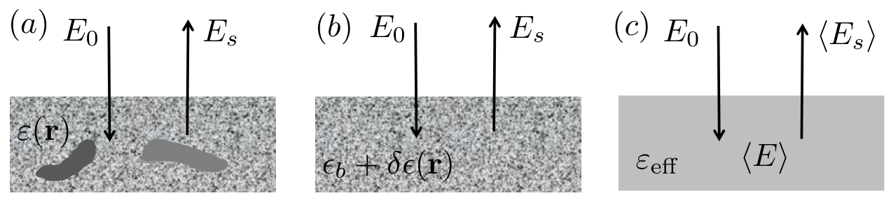
In the statistical approach, in which the scattering background is treated as a random medium, the scattered field is a random variable. In a given realization of the sample (deterministic large-scale objects immersed in one statistical realization of the scattering background), the total field can be written $E=\langle E\rangle+\delta E$. In OCT, one measures the backscattered field $E_{s}=E-E_{0}$, $E_{0}$ being the incident field, and we can also write $E_{s}=\langle E_{s}\rangle+\delta E_{s}$. In the regime of weak-scattering characterized by the condition $|\delta E_{s}|\ll|\langle E\rangle|$, multiple scattering in the background scattering medium can be described in the mean-field approximation. This approximation is based on well-established result in multiple scattering theory sheng2007introduction, that are summarized in Appendix A. In the mean-field approach, the fluctuating part $\delta E_{s}$ of the scattered field at point ${\bf r}_{D}$ in the detector plane, and at frequency $\omega$, reads

where $k_{0}=\omega/c$ is the wavenumber in free space, $\langle G({\bf r}_{D},{\bf r}^{\prime})\rangle$ is the average Green’s function connecting a point ${\bf r}^{\prime}$ in the sample to the detection point ${\bf r}_{D}$, and the integration is over the volume of the sample. Here the average Green’s function $\langle G\rangle$ and the average field $\langle E\rangle$ are defined as solutions of a propagation equation in an effective medium, described by an effective dielectric function $\varepsilon_{\mathrm{eff}}$, representing the average contribution of the random scattering background (the detailed derivation of Eq. (1) is given in Appendix A). It is important to note that this effective medium description is a rigorous result of multiple scattering theory sheng2007introduction; akkermans2007mesoscopic. Noting that $\Delta\varepsilon({\bf r}^{\prime})=\varepsilon({\bf r}^{\prime})-\varepsilon_{\mathrm{eff}}$ is the local dielectric contrast between a heterogeneity in the sample and the effective medium, a clear physical meaning can be given to Eq. (1): It expresses the fluctuating part $\delta E_{s}$ of the scattered field as the result of single scattering in the effective medium, a result valid in the weak-scattering regime $|\delta E_{s}|\ll|\langle E\rangle|$. The mean-field approach differs from the Born approximation by the renormalization of the background medium into an effective medium, that accounts in particular for the decay of the average Green’s function due to scattering, as we shall see. The average field is connected to the incident field $E_{0}$ in the source plane by the relation

where $\langle G({\bf r},{\bf r}_{S})\rangle$ is the average Green’s function connecting a point ${\bf r}_{S}=(\boldsymbol{\rho}_{S},z_{S})$ in the source plane to an arbitrary point ${\bf r}$, $A$ is a constant that we do not need to specify, and the integration is along the source plane. Inserting Eq. (2) into Eq. (1) leads to

In this expression, for the sake of clarity, we have denoted by $\langle G_{T}\rangle$ the Green’s function that accounts for propagation through the optics in the sample arm, transmission at the effective medium surface, and propagation inside the effective medium. The average scattered field at the detector is readily deduced from Eq. (2), and reads

Here, the average Green’s function $\langle G_{R}\rangle$ accounts for propagation through the optics in the sample arm, and reflection at the effective medium surface. For practical calculations, the average Green’s function in transmission or reflection can be approximated using a simple model, as we shall see below.

An OCT setup is based on a Michelson interferometer, as represented schematically in Fig. 2. Starting from the source, the beam is divided by a beam-splitter to travel along two arms. The sample arm collects the field backscattered from the sample. In the second arm, a reference beam is produced by reflection on a mirror. The detector collects the intensity resulting from the interference between the sample and reference beams. In FF-OCT, a full-field illumination is used in combination with an array of detectors (in practice a CCD camera) to record the signal at multiple transverse locations in parallel, and produce an en face image. This means that both arms contain a microscope objective, not represented in Fig. 2 for simplicity. The state of coherence of the light source plays a crucial role in FF-OCT. Beyond the longitudinal sectioning given by the temporal coherence length (or equivalently the spectral bandwidth), spatial coherence influences the lateral resolution, as well as the sensitivity to aberrations in the sample arm xiao2016full. In order to understand precisely the role of temporal and spatial coherence, we need to build a model of the FF-OCT signal that includes the scattering model introduced in the previous section, and the main features of the interferometric and broadband detection used in OCT.

Under illumination by statistically stationary light, the intensity recorded by a Michelson interferometer is characterized by three terms: The (time) average intensity of the reference field, the average intensity of the scattered field, and the cross-correlation between them (interference term). Assuming $|E_{s}|\ll|E_{0}|$, the signal carrying information on the sample is the interference term (the intensity of the scattered field is negligible, and the intensity of the reference field only contributes as a background signal) davis2007autocorrelation. In the frequency domain, the OCT signal measured at a given point ${\bf r}_{D}$ in the detector plane is

where $E_{\mathrm{ref}}$ and $E_{s}$ are, respectively, the complex amplitude of the reference and backscattered field at frequency $\omega$, the superscript $*$ denotes the complex conjugate, and the overline means a time averaging over the fluctuations of the partially coherent source.

The incident field $E_{0}$ at a point ${\bf r}=(\boldsymbol{\rho},z)$ can be written in the form of a plane-wave expansion

with $k_{z}(q)=(k_{0}^{2}-q^{2})^{1/2}$. The $z$-axis is chosen such that the plane $z=0$ coincides with the sample plane (the sample filling the half-space $z<0$), and the axis $z>0$ follows the optical axis in each arm (see Fig.1(d)). Assuming a weakly focused beam (the influence the numerical aperture is discussed in section V), we can perform a zeroth-order paraxial approximation $k_{z}(q)\simeq k_{0}$, resulting in $E_{0}({\bf r})=E_{0}(\boldsymbol{\rho},z=0)\exp(-ik_{0}z)$. The field in the reference arm is assumed to coincide with the incident field longitudinally shifted by the mirror displacement. Under the same paraxial approximation, we can write $E_{\mathrm{ref}}^{*}({\bf r}_{D})=E^{*}_{0}(\boldsymbol{\rho}_{D},z=0)\exp[-ik_{0}(z_{D}-2z_{0})]$ where $z_{0}$ is the position of the mirror along the $z$-axis in the reference arm and $z_{D}$ is the position of the detection plane along the $z$-axis in the detection arm. From Eqs. (3), (4), (5) and the expressions of $E_{0}$ and $E_{\mathrm{ref}}^{*}$ above , we can write the FF-OCT signal as

with

In these expressions we have introduced the cross-spectral density

that characterizes the state of coherence of the incident field in the sample plane $z=0$ mandel1995optical. Here we assume that the incoming intensity is uniform over the sample surface, and use a homogeneous Schell model such that $W_{0}$ is a function of $\boldsymbol{\rho}_{S}-\boldsymbol{\rho}_{D}$ only marks2009partially.

It is clear that $\langle S({\bf r}_{D},\omega)\rangle$ characterizes the effective medium, and does not carry information on $\Delta\varepsilon({\bf r}^{\prime})$. In order to build the simplest model, we assume weak scattering, meaning that $k_{0}\ell_{e}\gg 1$ with $\ell_{e}$ the extinction mean free path characterizing the decay of the average field (the exinction coefficient $\mu_{e}=1/\ell_{e}$ can also be used equivalently). The effective medium, as seen by the average field, is described by a dielectric function $\varepsilon_{\mathrm{eff}}=\varepsilon_{b}+i/(k_{0}\ell_{e})$ (this expression being valid to first order in the small parameter $1/(k_{0}\ell_{e})$) sheng2007introduction; akkermans2007mesoscopic. In this limit, the reflected average Green’s function $\langle G_{R}\rangle$ simply describes reflection at the surface of the effective medium, and contributes as a uniform background. Assuming a low index mismatch with $\varepsilon_{b}\simeq 1$, the contribution of $\langle S({\bf r}_{D},\omega)\rangle$ becomes negligible. In the following we focus on the contribution $\delta S({\bf r}_{D},\omega)$ that carry the relevant information on the image formation process. It is useful to introduce the plane-wave expansion of the average Green’s function:

We take $k_{z}(q)=(k_{0}^{2}-q^{2})^{1/2}$ for propagation outside the sample (for $z,z^{\prime}>0$), and $k_{z}(q)=k_{z}^{\mathrm{eff}}(q)=(\varepsilon_{\mathrm{eff}}k_{0}^{2}-q^{2})^{1/2}$ for propagation inside the sample (for $z,z^{\prime}<0$). The filter $g({\bf q})$ plays the role of a pupil function that limits the transverse wavevector ${\bf q}$ within a region bounded by the numerial aperture $NA$ of the objectives (the simplest model for $g({\bf q})$ is a disk with radius $k_{0}\,NA$) sentenac2018tutorial. For $g({\bf q})=1$ (infinite pupil), we recover the Weyl expansion of the free-space Green’s function. To get an expression of the FF-OCT signal relevant for an analysis in terms of optical transfer function, we insert Eq. (11) into Eq. (9), and perform again a zeroth-order paraxial approximation, using $k_{z}(q)\simeq k_{0}$ outside the sample, and $k_{z}^{\mathrm{eff}}(q)\simeq k_{0}+i/(2\ell_{e})$ inside the sample. The result is easily written in terms of the 2D Fourier transform of the signal, $\widetilde{\delta S}({\bf q},\omega)=\int\delta S({\bf r}_{D},\omega)\exp(-i{\bf q}\cdot\boldsymbol{\rho}_{D})d^{2}\rho_{D}/{4\pi^{2}}$, and reads

where $\widetilde{\Delta\varepsilon}({\bf q},z^{\prime})$ is the 2D Fourier transform of $\Delta\varepsilon(\boldsymbol{\rho}^{\prime},z^{\prime})$, and $\widetilde{W}_{0}({\bf q}^{\prime})$ is the 2D Fourier transform of $W_{0}({\boldsymbol{\rho}}_{S}-{\boldsymbol{\rho}}_{D})$. Note that $\widetilde{W}_{0}({\bf q}^{\prime})\propto{I}_{0}({\bf q}^{\prime})$, with $I_{0}({\bf q}^{\prime})$ the angular distribution of the incident intensity barabanenkov1968radiation; mandel1995optical. Also note that this expression does not rely on any assumption regarding the optics in the illumination, reference and detection arms, and does not depend on the definition of a focal plane for either illumination of detection (these features drive the precise form of the Green’s function $g({\bf q})$). In practice, in order to control the degree of spatial coherence in the sample plane $z=0$, one could choose to control the intensity distribution in the source plane $z=z_{S}$ and conjugate this plane with the plane $z=0$, but this practical choice does not influence the general form of Eq. (12).

A feature of OCT is to integrate the signal over a broad spectral range. For a statistically stationary source, the broadband signal is obtained by integrating the different frequency components over the source bandwidth $\Delta\omega$. Assuming that $W_{0}$ and $\Delta\varepsilon$ have a weak dependence on $\omega$, the spectral integration gives

where $\bar{k}_{0}=\omega_{0}/c$, with $\omega_{0}$ the central frequency of the source. The $\mathrm{sinc}$ function, considered as a function of $z^{\prime}$, is centered at $z_{0}$ with a width $\ell_{\omega}=c/\Delta\omega$ corresponding to the temporal coherence length of the incident light, and is responsible for the longitudinal sectioning in OCT. When $\ell_{\omega}\ll\ell_{e}$, we can use the approximation $\mathrm{sinc}[(z_{0}-z^{\prime})/\ell_{\omega}]\simeq\pi\ell_{\omega}\delta(z_{0}-z^{\prime})$. We endup with a closed-form expression of the 2D Fourier transform of the broadband OCT signal $\widetilde{\delta S}({\bf q})=\int_{\Delta\omega}\widetilde{\delta S}({\bf q},\omega)d\omega$, that depends on the position $z_{0}$ of the mirror and on the source bandwith $\Delta\omega$:

Expression (14) of the the FF-OCT signal implicitly involves different length scales, whose interplay is critical in the analysis of the signal: The length scale $\ell_{\varepsilon}$ characterizing the microscopic random inhomogeneities in the sample, the length scale $L_{\varepsilon}$ characterizing large-scale deterministic fluctuations of the dielectric function, the temporal coherence length $\ell_{\omega}$ and the spatial coherence length $\ell_{c}$ of the incident light. Expression (14) is similar to that previously derived in Ref. marks2009partially. The main difference is that our derivation includes a scattering model based on a mean-field approach, that only relies on the weak-scattering assumption $|\delta E_{s}|\ll|\langle E\rangle|$, always satisfied when the scattered field remains much smaller than the incident field. This approach goes beyond a first-order or second-order Born approximation, by accounting rigorously for the propagation of the average field in a renormalized effective medium. An interesting consequence is that the extinction of the signal with depth, due to scattering and absorption, emerges explicitly.

Expression (14) is an interesting starting point for the analysis of the role of spatial coherence on the image formation in FF-OCT. To proceed, let us rewrite it in the compact form

where $\widetilde{H}({\bf q})\sim\int d^{2}q^{\prime}g({\bf q}^{\prime})g({\bf q}+{\bf q}^{\prime})\widetilde{W}_{0}({\bf q}^{\prime})$ is the FF-OCT transfer function (we omit constant prefactors for simplicity), and $\widetilde{\Delta\varepsilon}_{z_{0}}({\bf q})=\widetilde{\Delta\varepsilon}({\bf q},z_{0})\exp(-z_{0}/\ell_{e})$ is the weighted 2D Fourier transform of the dielectric contrast. The width of the cross-spectral density $W_{0}(\boldsymbol{\rho})$ defines the spatial coherence length $\ell_{c}$ of the incident field in the sample plane $z=0$. When $\ell_{c}\gg L_{\varepsilon}\gg\ell_{\varepsilon}$, the incident light can be considered fully coherent, which corresponds to $\widetilde{W}_{0}({\bf q}^{\prime})\sim I_{0}\delta({\bf q}^{\prime})$, $I_{0}$ being proportionnal to the incident intensity. The transfer function for spatially coherent illumination becomes

The coherent transfer function $\widetilde{H}_{c}({\bf q})$ posseses the same spatial frequency content as $g({\bf q})$, and covers the spatial frequency range $q\leq\bar{k}_{0}NA$, leading to a transverse spatial resolution limit $\lambda/(2NA)$, where $\lambda=2\pi/\bar{k}_{0}$ is the central wavelength of the incident field. The regime of spatially incoherent illumination corresponds formally to $W_{0}(\boldsymbol{\rho})\sim\delta(\boldsymbol{\rho})$, or equivalently $\widetilde{W}_{0}({\bf q}^{\prime})=I_{0}^{\prime}$. The transfer function for spatially incoherent illumination reads as

In practice, since $\ell_{c}$ cannot be made smaller than $\lambda/2$ under far-field illumination, the condition $\ell_{c}\ll\ell_{\varepsilon}\ll L_{\varepsilon}$ that rigorously corresponds to $W_{0}(\boldsymbol{\rho})\sim\delta(\boldsymbol{\rho})$ is out of reach. Nevertheless, provided that FF-OCT is used to image the large-scale inhomonegeities at the scale $L_{\varepsilon}$, and not to resolve the small-scale random scattering centers, the condition of incoherent illumination can be relaxed to be $\ell_{c}\simeq\ell_{\varepsilon}\ll L_{\varepsilon}$. The integral term in Eq. (17) shows that the spatial frequency range encompassed by $\widetilde{H}_{i}({\bf q})$ is broader by a factor of two compared to coherent illumination, which is a usual result in optical microscopy, leading to a theoretical resolution limit $\lambda/(4NA)$. The results above, for coherent and incoherent illumination, are identical to those previsouly established in Ref. marks2009partially, and in agreement with the qualitative analysis of coherent and incoherent FF-OCT presented in Ref. sentenac2018tutorial.

Expressions (16) and (17) may also provide a theoretical frame to study the influence of aberrations in the sample arm on the image quality, recently discussed in Ref. xiao2016full. A precise study is beyond the scope of the present work. Qualitatively, we can simply note that weak aberrations that would tend to squeeze the Green’s function $g({\bf q})$ in Fourier space (without changing the cutoff frequency) would narrow the shape of $\widetilde{H}_{c}({\bf q})$, thus degrading the image quality. For incoherent illumination, the convolution product in Eq. (17) reduces the sensitivity of the transfer function to change in shapes due to weak aberrations, resulting in a better protection of the image quality.

The decay of the signal with depth is a feature of OCT. For paraxial illumination and detection, and in a medium with $\widetilde{\Delta\varepsilon}({\bf q},z_{0})$ independent of $z_{0}$, the signal follows an exponential decay $\exp(-z_{0}/\ell_{e})$, as described by Eq. (14). This exponential decay can be used for the measurement of the extinction length in weakly scattering materials plamann2019OCT. At higher numerical aperture, a correction to a pure exponential decay is expected, that may also depend on the degree of spatial coherence of the incident field. To address this question, we make use of a second-order paraxial approximation

in the plane-wave expansions of the incident field [Eq. (6)] and of the average Green’s function [Eq. (11)]. Note that, as a result of the mean-field approach, the paraxial approximation in the scattering medium amounts to replacing $k_{0}$ by $\sqrt{\varepsilon_{\mathrm{eff}}}k_{0}$. This strongly influences the dependence of the FF-OCT on the numerical aperture, as we shall see. Following again the steps leading to Eq. (14), we end up with an expression of the FF-OCT signal that explicitely accounts for the angular aperture of the illumination and detection beams. In order to discuss the depth dependence of the spatially integrated signal, we consider $\widetilde{\delta S}({\bf q}=0)$, which can be cast in the following form (details of the derivation are given in Appendix B):

where $\bar{k}_{0}=\omega_{0}/c$ is the central wavenumber of the polychromatic incident field. This expression is well suited to a discussion of the depth dependence of the integrated FF-OCT signal. Note that in practice, an exponential fit to the signal is often used to estimate the extinction mean free path $\ell_{e}$ in statistically homogeneous and isotropic scattering media. From Eq. (20), it is clear that at finite $NA$ a deviation from a pure exponential decay $\exp(-z_{0}/\ell_{e})$ may be observed due to the dependence on $z_{0}$ of the integral over $q^{\prime}$. This integral contains several cutoffs. First, the last exponential term gives a depth-dependent cutoff $q^{\prime}_{z_{0}}\simeq\bar{k}_{0}(\ell_{e}/z_{0})^{1/2}$. For $z_{0}\gg\ell_{e}$, the integral is restricted to vanishingly small $q^{\prime}$, and a pure exponential decay $\exp(-z_{0}/\ell_{e})$ is always expected in the tail of the signal versus depth. Second, the angular spectrum of the Green’s function $g({\bf q}^{\prime})$ produces a cutoff $q^{\prime}_{NA}\simeq\bar{k}_{0}NA$, showing that for $NA\to 0$ a pure exponential decay is observed, in agreement with Eq. (14). Third, the Fourier transform of the cross spectral density $\widetilde{W}_{0}({\bf q}^{\prime})$ introduces a cutoff $q^{\prime}_{c}\simeq 2\pi/\ell_{c}$ that depends on the degree of spatial coherence of the incident light in the sample plane. For $\ell_{c}\to\infty$ (spatially coherent illumination), a pure exponential decay is also observed. More precisely, to prevent the $\exp[-q^{\prime 2}z_{0}/(2\bar{k}_{0}^{2}\ell_{e})]$ term in the integral to play a role, we need either $NA\ll(\ell_{e}/z_{0})^{1/2}$ (low numerical aperture regime), or $\ell_{c}\gg\lambda(z_{0}/\ell_{e})^{1/2}$ (coherent illumination).

This qualitative analysis is confirmed by numerical calculations of the spatially integrated signal using Eq. (20), as shown in Fig. 3. A non-exponential decay is observed in the regime $NA\simeq(\ell_{e}/z_{0})^{1/2}\simeq\lambda/\ell_{c}$. The deviation from a pure exponential decay is enhanced at high $NA$ and low spatial coherence. Although the curves are displayed in the regime $z_{0}\simeq\ell_{e}$, we have verified that an exponential decay $\exp(-z_{0}/\ell_{e})$ is recovered in any case when $z_{0}\gg\ell_{e}$. Numerical calculations based on ab initio simulations could extend the analysis beyond the weak-scattering regime and second-order paraxial approximations used in this model. This is left for future work.

In summary, we have developed a model of FF-OCT that includes a mean-field scattering theory, in addition to a precise description of temporal and spatial coherence. The model describes the decay of the signal with depth due to scattering and absorption, an essential feature in OCT imaging. It also permits an analysis of the interplay between different length scales characterizing the scattering medium and the degree of coherence of the incident field. Based on explicit expressions of the FF-OCT signal, we have discussed several features of FF-OCT imaging. We have analyzed the influence of spatial coherence on the optical transfer function, and discussed the particular cases of fully coherent and incoherent illuminations. We have also studied the depth dependence of the signal integrated over the transverse directions, that not only limits the penetration depth in OCT, but is also used to measure the extinction length in scattering materials. For spatially incoherent illumination, and/or with high numerical aperture of the illumination/detection optics, deviations from a pure exponential decay $\exp(-z_{0}/\ell_{e})$ can be observed. A pure exponential decay is always recovered in the tail of the signal versus depth when $z_{0}\gg\ell_{e}$. Our analysis provides a clear frame for the use of the Beer-Lambert law for quantitative measurements of the extinction length in scattering media. The model also provides a framework for a precise analysis of the role of aberrations generated by the optics in the sample arm, or by the scattering medum itself, and for the development of advanced inverse reconstruction procedures going beyond the first and second-order Born approximations.

This work was supported by the European Union’s Seventh Framework Program under HELMHOLTZ grant agreement No 610110, and by LABEX WIFI (Laboratory of Excellence ANR-10-LABX-24) within the French Program “Investments for the Future” under reference ANR-10-IDEX-0001-02 PSL^∗.

We thank A. Aubry, V. Barolle, C. Boccara, R. Bocheux, K. Irsch and K. Plamann for stimulating discussions.

References

- (1) D. Huang, E. A. Swanson, C. P. Lin, J. S. Schuman, W. G. Stinson, W. Chang, M. R. Hee, T. Flotte, K. Gregory, C. A. Puliafito et al., “Optical coherence tomography,” Science 254, 1178–1181 (1991).
- (2) J. M. Schmitt, “Optical coherence tomography (oct): a review,” IEEE J. Select. Topics Quantum Electron. 5, 1205–1215 (1999).
- (3) A. F. Fercher, W. Drexler, C. K. Hitzenberger, and T. Lasser, “Optical coherence tomography-principles and applications,” Rep. Prog. Phys. 66, 239 (2003).
- (4) N. Nassif, B. Cense, B. H. Park, S. H. Yun, T. C. Chen, B. E. Bouma, G. J. Tearney, and J. F. de Boer, “In vivo human retinal imaging by ultrahigh-speed spectral domain optical coherence tomography,” Opt. Lett. 29, 480–482 (2004).
- (5) R. Huber, M. Wojtkowski, and J. Fujimoto, “Fourier domain mode locking (fdml): A new laser operating regime and applications for optical coherence tomography,” Opt. express 14, 3225–3237 (2006).
- (6) B. M. Hoeling, A. D. Fernandez, R. C. Haskell, E. Huang, W. R. Myers, D. C. Petersen, S. E. Ungersma, R. Wang, M. E. Williams, and S. E. Fraser, “An optical coherence microscope for 3-dimensional imaging in developmental biology,” Opt. Express 6, 136–146 (2000).
- (7) Y. Zhang, J. Rha, R. S. Jonnal, and D. T. Miller, “Adaptive optics parallel spectral domain optical coherence tomography for imaging the living retina,” Opt. Express 13, 4792–4811 (2005).
- (8) S. Bourquin, P. Seitz, and R. Salathé, “Optical coherence topography based on a two-dimensional smart detector array,” Opt. Lett. 26, 512–514 (2001).
- (9) E. Bordenave, E. Abraham, G. Jonusauskas, N. Tsurumachi, J. Oberle, C. Rulliere, P. Minot, M. Lassegues, and J. S. Bazeille, “Wide-field optical coherence tomography: imaging of biological tissues,” Appl. Opt. 41, 2059–2064 (2002).
- (10) M. Laubscher, M. Ducros, B. Karamata, T. Lasser, and R. Salathe, “Video-rate three-dimensional optical coherence tomography,” Opt. Express 10, 429–435 (2002).
- (11) L. Vabre, A. Dubois, and A. C. Boccara, “Thermal-light full-field optical coherence tomography,” Opt. Lett. 27, 530–532 (2002).
- (12) A. Fercher, C. Hitzenberger, M. Sticker, E. Moreno-Barriuso, R. Leitgeb, W. Drexler, and H. Sattmann, “A thermal light source technique for optical coherence tomography,” Opt. Commun. 185, 57–64 (2000).
- (13) J. M. Schmitt and A. Knüttel, “Model of optical coherence tomography of heterogeneous tissue,” J. Opt. Soc. Am. A 14, 1231–1242 (1997).
- (14) R. H. Webb, “Confocal optical microscopy,” Rep. Prog. Phys. 59, 427 (1996).
- (15) M. R. Hee, J. A. Izatt, J. M. Jacobson, J. G. Fujimoto, and E. A. Swanson, “Femtosecond transillumination optical coherence tomography,” Opt. Lett. 18, 950–952 (1993).
- (16) J. Schmitt, A. Gandjbakhche, and R. Bonner, “Use of polarized light to discriminate short-path photons in a multiply scattering medium,” Appl. Opt. 31, 6535–6546 (1992).
- (17) C. M. Macdonald, U. Tricoli, A. Da Silva, and V. A. Markel, “Numerical investigation of polarization filtering for direct optical imaging within scattering media,” J. Opt. Soc. Am. A 34, 1330–1338 (2017).
- (18) D. L. Marks, B. J. Davis, S. A. Boppart, and P. S. Carney, “Partially coherent illumination in full-field interferometric synthetic aperture microscopy,” J. Opt. Soc. Am. A 26, 376–386 (2009).
- (19) S. G. Adie, B. W. Graf, A. Ahmad, P. S. Carney, and S. A. Boppart, “Computational adaptive optics for broadband optical interferometric tomography of biological tissue,” Proc. Natl. Acad. Sci. (USA) (2012).
- (20) P. Xiao, M. Fink, and A. C. Boccara, “Full-field spatially incoherent illumination interferometry: a spatial resolution almost insensitive to aberrations,” Optics letters 41, 3920–3923 (2016).
- (21) A. Badon, D. Li, G. Lerosey, A. C. Boccara, M. Fink, and A. Aubry, “Smart optical coherence tomography for ultra-deep imaging through highly scattering media,” Science advances 2, e1600370 (2016).
- (22) A. Badon, A. C. Boccara, G. Lerosey, M. Fink, and A. Aubry, “Multiple scattering limit in optical microscopy,” Opt. Express 25, 28914–28934 (2017).
- (23) P. Sheng, Introduction to Wave Scattering, Localization and Mesoscopic Phenomena (Springer, 2010).
- (24) E. Akkermans and G. Montambaux, Mesoscopic Physics of Electrons and Photons (Cambridge University Press, 2007).
- (25) B. J. Davis, T. S. Ralston, D. L. Marks, S. A. Boppart, and P. S. Carney, “Autocorrelation artifacts in optical coherence tomography and interferometric synthetic aperture microscopy,” Opt. Lett. 32, 1441–1443 (2007).
- (26) L. Mandel and E. Wolf, Optical Coherence and Quantum Optics (Cambridge University Press, 1995).
- (27) A. Sentenac and J. Mertz, “Unified description of three-dimensional optical diffraction microscopy: from transmission microscopy to optical coherence tomography: tutorial,” J. Opt. Soc. Am. A 35, 748–754 (2018).
- (28) Y. N. Barabanenkov and V. Finkelberg, “Radiation transport equation for correlated scatterers,” Sov. Phys. JETP 26, 587–591 (1968).
- (29) R. Bocheux, P. Pernot, V. Borderie, K. Plamann and K. Irsch, “Quantitative measures of corneal transparency, derived from objective analysis of depth-resolved corneal images, demonstrated with full-field optical coherence tomographic microscopy,” PLoS ONE 14, e0221707 (2019).