跳到论文正文
W Papers独立论文阅读器 arXiv:1908.01034 论文正文 计算阅读时间 · 0%
引用这篇论文根据当前论文元数据生成,正式投稿前建议核对。


License: arXiv.org perpetual non-exclusive license
arXiv:1908.01034v1 [math.ST] 02 Aug 2019

Efficient Truncated Statistics with Unknown Truncation

Vasilis Kontonis Affiliation: UW Madison Email: kontonis@wisc.edu    Christos Tzamos Affiliation: UW Madison Email: tzamos@wisc.edu    Manolis Zampetakis Affiliation: MIT Email: mzampet@mit.edu
Abstract

We study the problem of estimating the parameters of a Gaussian distribution when samples are only shown if they fall in some (unknown) subset S⊆ℝdS\subseteq\mathbb{R}^{d}. This core problem in truncated statistics has long history going back to Galton, Lee, Pearson and Fisher. Recent work by Daskalakis et al. (FOCS’18), provides the first efficient algorithm that works for arbitrary sets in high dimension when the set is known, but leaves as an open problem the more challenging and relevant case of unknown truncation set.

Our main result is a computationally and sample efficient algorithm for estimating the parameters of the Gaussian under arbitrary unknown truncation sets whose performance decays with a natural measure of complexity of the set, namely its Gaussian surface area. Notably, this algorithm works for large families of sets including intersections of halfspaces, polynomial threshold functions and general convex sets. We show that our algorithm closely captures the tradeoff between the complexity of the set and the number of samples needed to learn the parameters by exhibiting a set with small Gaussian surface area for which it is information theoretically impossible to learn the true Gaussian with few samples.

1 Introduction

A classical challenge in Statistics is estimation from truncated samples. Truncation occurs when samples falling outside of some subset SS of the support of the distribution are not observed. Truncation of samples has myriad manifestations in business, economics, engineering, social sciences, and all areas of the physical sciences.

Statistical estimation under truncated samples has had a long history in Statistics, going back to at least the work of Galton [Gal97] who analyzed truncated samples corresponding to speeds of American trotting horses. Following Galton’s work, Pearson and Lee [Pea02, PL08, Lee14] used the method of moments in order to estimate the mean and standard deviation of a truncated univariate normal distribution and later Fisher [Fis31] used the maximum likelihood method for the same estimation problem. Since then, there has been a large volume of research devoted to estimating the truncated normal distribution; see e.g. [Sch86, Coh16, BC14]. Nevertheless, the first algorithm that is provably computationally and statistically efficient was only recently developed by Daskalakis et al. [DGTZ18], under the assumption that the truncation set SS is known.

In virtually all these works the question of estimation under unknown truncation set is raised. Our work resolves this question by providing tight sample complexity guarantees and an efficient algorithm for recovering the underlying Gaussian distribution. Although this estimation problem has clear and important practical and theoretical motivation too little was known prior to our work even in the asymptotic regime. In the early work of Shah and Jaiswal [SJ66] it was proven that the method of moments can be used to estimate a single dimensional Gaussian distribution when the truncation set is unknown but it is assumed to be an interval. In the other extreme where the set is allowed to be arbitrarily complex, Daskalakis et al. [DGTZ18] showed that it is information theoretically impossible to recover the parameters. We provide the first complete analysis of the number of samples needed for recovery taking into account the complexity of the underlying set.

Our Contributions.

Our work studies the estimation task when the truncation set belongs in a family 𝒞\mathcal{C} of “low complexity”. We use two different notions for quantifying the complexity of sets: the VC-dimension and the Gaussian Surface Area.

Our first result is that for any set family with VC-dimension VC⁡(𝒞)\mathrm{VC}(\mathcal{C}), the mean and covariance of the true dd-dimensional Gaussian Distribution can be recovered up to accuracy ε\varepsilon using only O~​(VC⁡(𝒞)ε+d2ε2)\tilde{O}\left(\frac{\mathrm{VC}(\mathcal{C})}{\varepsilon}+\frac{d^{2}}{\varepsilon^{2}}\right) truncated samples.

Informal Theorem 1.

Let 𝒞\mathcal{C} be a class of sets with VC-dimension VC⁡(𝒞)\mathrm{VC}(\mathcal{C}) and let N=O~​(VC⁡(𝒞)ε+d2ε2)N=\tilde{O}\left(\frac{\mathrm{VC}(\mathcal{C})}{\varepsilon}+\frac{d^{2}}{\varepsilon^{2}}\right). Given NN samples from a dd-dimensional Gaussian 𝒩⁡(𝛍,𝚺)\mathcal{N}(\bm{\mu},\bm{\Sigma}) with unknown mean μ\mu and covariance 𝚺\bm{\Sigma}, truncated on a set S∈𝒞S\in\mathcal{C} with mass at least α\alpha, it is possible to find an estimate (𝛍^,𝚺^)(\hat{\bm{\mu}},\hat{\bm{\Sigma}}) such that dTV​(𝒩⁡(𝛍,𝚺),𝒩⁡(𝛍^,𝚺^))≤εd_{\mathrm{TV}}(\mathcal{N}(\bm{\mu},\bm{\Sigma}),\mathcal{N}(\hat{\bm{\mu}},\hat{\bm{\Sigma}}))\leq\varepsilon.

The estimation method computes the set of smallest mass that maximizes the likelihood of the data observed and learns the truncated distribution within error O⁡(ε)O(\varepsilon) in total variation distance. To translate this error in total variation to parameter distance, we prove a general result showing that it is impossible to create a set (no matter the complexity) so that two Gaussians whose parameters are far have similar truncated distributions (see Lemma 3).

A simple but not successful approach would be to first try to learn an approximation of the truncation set with symmetric difference roughly ε2/d2\varepsilon^{2}/d^{2} with the true set and then run the algorithm of [DGTZ18] using the approximate oracle. This approach would lead to a VC⁡(𝒮)​d2/ε2\mathrm{VC}(\mathcal{S})d^{2}/\varepsilon^{2} sample complexity that is worse than what we get. More importantly, doing empirical risk minimization11 1 That is finding a set of the family that contains all the observed samples. using truncated samples does not guarantee that we will find a set of small symmetric difference with the true and it is not clear how one could achieve that.

Our result bounds the sample complexity of identifying the underlying Gaussian distribution in terms of the VC-dimension of the set but does not yield a computationally efficient method for recovery. Obtaining a computationally efficient algorithm seems unlikely, unless one restricts attention to simple specific set families, such as axis aligned rectangles. One would hope that exploiting the fact that samples are drawn from a “tame” distribution, such as a Gaussian, can lead to general computationally efficient algorithms and even improved sample complexity.

Indeed, our main result is an algorithm that is both computationally and statistically efficient for estimating the parameters of a spherical Gaussian and uses only dO​(Γ2​(𝒞))d^{O(\Gamma^{2}(\mathcal{C}))} samples, where Γ⁡(𝒞)\Gamma(\mathcal{C}) is the Gaussian Surface Area of the class 𝒞\mathcal{C}, an alternative complexity measure introduced by Klivans et al. [KOS08]:

Informal Theorem 2.

Let 𝒞\mathcal{C} be a class of sets with Gaussian surface area at most Γ⁡(𝒞)\Gamma(\mathcal{C}) and let k=poly(1/α,1/ε)Γ(𝒞)2k=\poly(1/\alpha,1/\varepsilon)\Gamma(\mathcal{C})^{2}. Given N=dkN=d^{k} samples from a spherical dd-dimensional Gaussian 𝒩⁡(𝛍,σ2​𝐈)\mathcal{N}(\bm{\mu},\sigma^{2}\bm{I}), truncated on a set S∈𝒞S\in\mathcal{C} with mass at least α\alpha,in time poly(m)\poly(m), we can find an estimate μ^,σ^2\hat{\mu},\hat{\sigma}^{2} such that

dTV​(𝒩⁡(𝝁,σ2​𝑰),𝒩⁡(𝝁^,σ^2​𝑰))≤ε.d_{\mathrm{TV}}(\mathcal{N}(\bm{\mu},\sigma^{2}\bm{I}),\mathcal{N}(\hat{\bm{\mu}},\hat{\sigma}^{2}\bm{I}))\leq\varepsilon.

The notion of Gaussian surface area can lead to better sample complexity bounds even when the VC dimension is infinite. An example of such a case is when 𝒞\mathcal{C} is the class of all convex sets. Table 1 summarizes the known bounds for the Gaussian surface area of different concept classes and the implied sample complexity in our setting when combined with our main theorem.

Concept Class Gaussian Surface Area Sample Complexity
Polynomial threshold functions of degree kk O⁡(k)O(k) [Kan11] dO⁡(k2)d^{O(k^{2})}
Intersections of kk halfspaces O⁡(log⁡k)O(\sqrt{\log{k}}) [KOS08] dO⁡(log⁡k)d^{O(\log k)}
General convex sets O⁡(d1/4)O(d^{1/4}) [Bal93] dO⁡(d)d^{O(\sqrt{d})}
Table 1: Summary of known results for Gaussian Surface Area. The last column gives the sample complexity we obtain for our setting.

Beyond spherical Gaussians, our main result extends to Gaussians with arbitrary diagonal covariance matrices. In addition, we provide an information theoretic result showing that the case with general covariance matrices can also be estimated using the same sample complexity bound by finding a Gaussian and a set that matches the moments of the true distribution. We remark our main algorithmic result Informal Theorem 3 uses Gaussian Surface Area whereas our sample complexity result Informal Theorem 2 uses VC-dimension. We discuss the differences of the two approaches in Section 7.

Informal Theorem 3.

Let 𝒞\mathcal{C} be a class of sets with Gaussian surface area at most Γ⁡(𝒞)\Gamma(\mathcal{C}) and let k=poly(1/α,1/ε)Γ(𝒞)2k=\poly(1/\alpha,1/\varepsilon)\Gamma(\mathcal{C})^{2}. Any truncated Gaussian with 𝒩⁡(𝛍^,𝚺^,S^)\mathcal{N}(\hat{\bm{\mu}},\hat{\bm{\Sigma}},\hat{S}) with S^∈𝒞\hat{S}\in\mathcal{C} that approximately matches the moments up to degree kk of a truncated dd-dimensional Gaussian 𝒩⁡(𝛍,𝚺,S)\mathcal{N}(\bm{\mu},\bm{\Sigma},S) with S∈𝒞S\in\mathcal{C}, satisfies dTV​(𝒩⁡(𝛍,𝚺),𝒩⁡(𝛍^,𝚺^))≤εd_{\mathrm{TV}}(\mathcal{N}(\bm{\mu},\bm{\Sigma}),\mathcal{N}(\hat{\bm{\mu}},\hat{\bm{\Sigma}}))\leq\varepsilon. The number of samples to estimate the moments within the required accuracy is at most dO⁡(k)d^{O(k)}.

This shows that the first few moments are sufficient to identify the parameters. Analyzing the guarantees of moment matching methods is notoriously challenging as it involves bounding the error of a system of many polynomial equations. Even for a single-dimensional Gaussian with truncation in an interval, where closed form solutions of the moments exist, it is highly non-trivial to bound these errors [SJ66]. In contrast, our analysis using Hermite polynomials allows us to easily obtain bounds for arbitrary truncation sets in high dimensions, even though no closed form expression for the moments exists.

We conclude by showing that the dependence of our sample complexity bounds both on the VC-dimension and the Gaussian Surface Area is tight up to polynomial factors. In particular, we construct a family in dd dimensions with VC dimension 2d2^{d} and Gaussian surface area O⁡(d)O(d) for which it is not possible to learn the mean of the underlying Gaussian within 1 standard deviation using o⁡(2d/2)o(2^{d/2}) samples.

Informal Theorem 4.

There exists a family of sets 𝒮\mathcal{S} with Γ⁡(𝒮)=O⁡(d)\Gamma({\mathcal{S}})=O(d) and VC-dimension 2d2^{d} such that any algorithm that draws NN samples from 𝒩⁡(𝛍,𝐈,S)\mathcal{N}(\bm{\mu},\bm{I},S) and computes an estimate 𝛍~\widetilde{\bm{\mu}} with ‖𝛍~−𝛍‖2≤1\left\|\widetilde{\bm{\mu}}-\bm{\mu}\right\|_{2}\leq 1 must have N=Ω⁡(2d/2)N=\Omega(2^{d/2}).

Our techniques and relation to prior work.

The work of Klivans et al. [KOS08] provides a computationally and sample efficient algorithm for learning geometric concepts from labeled examples drawn from a Gaussian distribution. On the other hand, the recent work of Daskalakis et al. [DGTZ18] provides efficient estimators for truncated statistics with known sets. One could hope to combine these two approaches for our setting, by first learning the set and then using the algorithm of [DGTZ18] to learn the parameters of the Gaussian. This approach, however, fails for two reasons. First, the results of Klivans et al. [KOS08] apply in the supervised learning setting where one has access to both positive and negative samples, while our problem can be thought of as observing only positive examples (those falling inside the set). In addition, any direct approach that extends their result to work with positive only examples requires that the underlying Gaussian distribution is known in advance.

One of our key technical contributions is to extend the techniques of Klivans et al. [KOS08] to work with positive only examples from an unknown Gaussian distribution, which is the major case of interest in truncated statistics. To perform the set estimation Klivans et al. [KOS08], rely on a family of orthogonal polynomials with respect to the Gaussian distribution, namely the Hermite polynomials and show that the indicator function of the set is well approximated by its low degree Hermite expansion. While we cannot learn this function directly in our setting, we are able to recover an alternative function, that contains “entangled” information of both the true Gaussian parameters and the underlying set. After learning the function, we formulate an optimization problem whose solution enables us to decouple these two quantities and retrieve both the Gaussian parameters and the underlying set. We describe our estimation method in more detail in Section 4. As a corollary of our approach, we obtain the first efficient algorithm for learning geometric concepts from positive examples drawn from an unknown spherical Gaussian distribution.

Simulations.

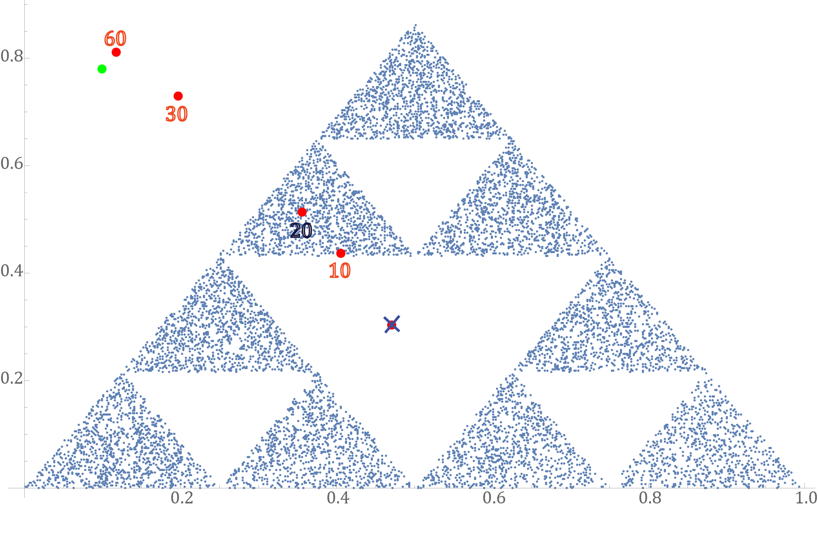
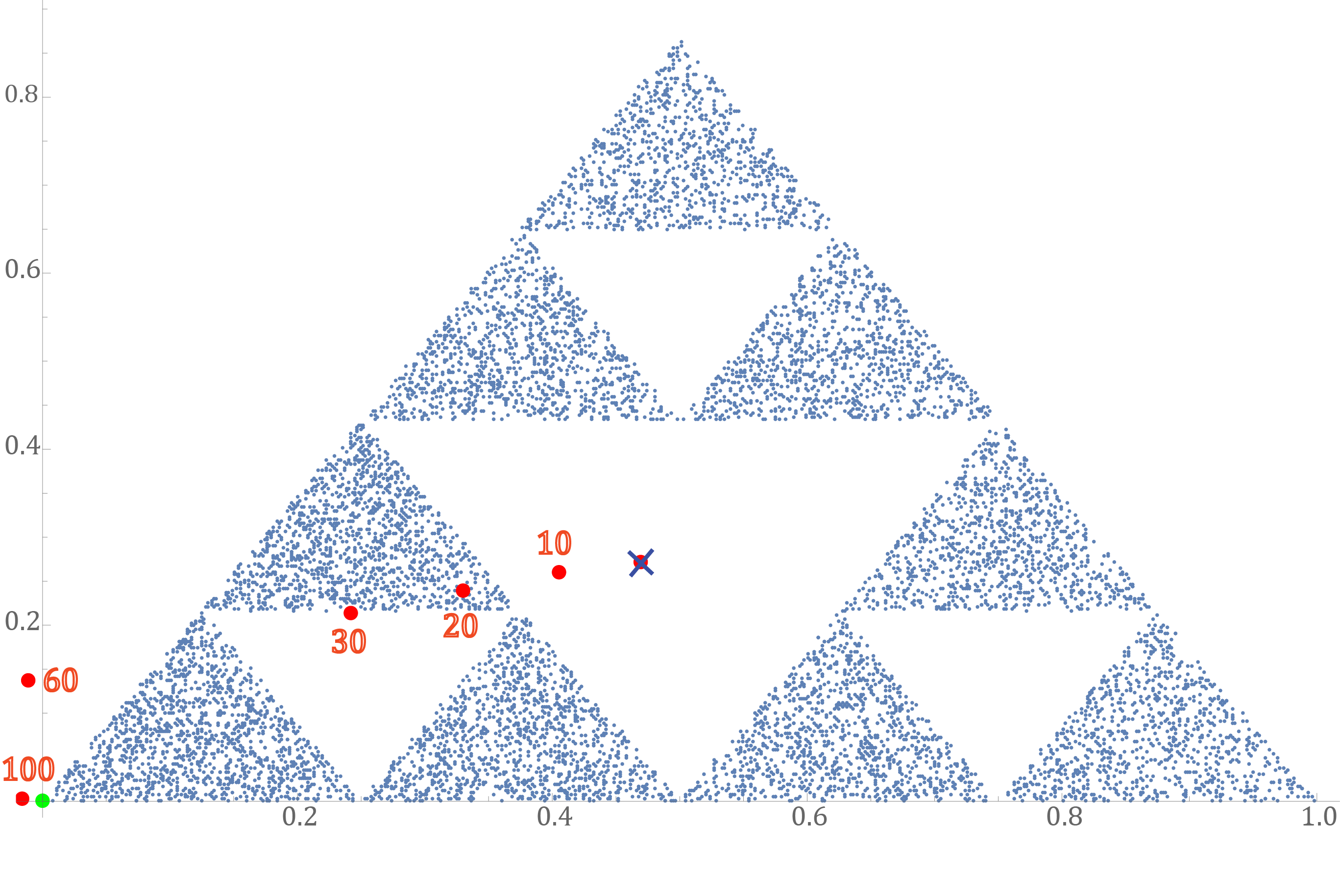
In addition to the theoretical guarantees of our algorithm, we empirically evaluate its performance using simulated data. We present the results that we get in Figure 1, where one can see that even when the truncation set is complex, our algorithm finds an accurate estimation of the mean of the untruncated distribution. Observe that our algorithm succeeds in estimating the true mean of the input distribution despite the fact that the set is unknown and the samples look similar in both cases.
Refer to caption
(a) Execution of our algorithm for isotropic Gaussian distribution with 𝝁∗=(0.1,0.78)\bm{\mu}^{*}=(0.1,0.78) and 𝝁S=(0.48,0.32)\bm{\mu}_{S}=(0.48,0.32).
Refer to caption
(b) Execution of our algorithm for isotropic Gaussian distribution with 𝝁∗=(0,0)\bm{\mu}^{*}=(0,0) and 𝝁S=(0.47,0.27)\bm{\mu}_{S}=(0.47,0.27).
Figure 1: Illustration of the results of our algorithm for an unknown truncation set. The ×\times sign corresponds to the conditional mean of the truncated distribution, while the green point corresponds to the true mean and the red points correspond to the estimated true mean depending on the degree of the Hermite polynomials that are being used by the algorithm.

1.1 Further Related Work

Our work is related to the field of robust statistics as it can robustly learn a Gaussian even in the presence of an adversary erasing samples outside a certain set. Recently, there has been a lot of theoretical work doing robust estimation of the parameters of multi-variate Gaussian distributions in the presence of arbitrary corruptions to a small ε\varepsilon fraction of the samples, allowing for both deletions of samples and additions of samples that can also be chosen adaptively [DKK+16, CSV17, LRV16, DKK+17, DKK+18]. When the corruption of the data is so powerful it is easy to see that the estimation error of the parameter depends on ε\varepsilon and cannot shrink to 00 as the number of samples grows to infinity. In our model the corruption is more restrictive but in return our results show how to estimate the parameters of a multi-variate Gaussian distribution to arbitrary accuracy even when the fraction of corruption is any constant less than 11.

Our work also has connections with the literature of learning from positive examples. At the heart of virtually all of the results in this literature is the use of the exact knowledge of the original non-truncated distribution to be able to generate fake negative examples, e.g. [Den98, LDG00]. When the original distribution is uniform, better algorithms are known. Diakonikolas et al. [DDS14] gave efficient learning algorithms for DNFs and linear threshold functions, Frieze et al. [FJK96] and Anderson et al. [AGR13] gave efficient learning algorithms for learning dd-dimensional simplices. Another line of work proves lower bounds on the sample complexity of recovering an unknown set from positive examples. Goyal et al. [GR09] showed that learning a convex set in dd-dimensions to accuracy ε\varepsilon from positive samples, uniformly distributed inside the set, requires at least 2Ω⁡(d/ε)2^{\Omega(\sqrt{d/\varepsilon})} samples, while the work of [Eld11] showed that 2Ω⁡(d)2^{\Omega(\sqrt{d})} samples are necessary even to estimate the mass of the set. To the best of our knowledge, no matching upper bounds are known for those results. Our estimation result implies that dpoly(1ε)dd^{\poly(\frac{1}{\varepsilon})\sqrt{d}} are sufficient to learn the set and its mass when given positive samples from a Gaussian truncated on the convex set.

2 Preliminaries

Notation. We use small bold letters 𝒙\bm{x} to refer to real vectors in finite dimension ℝd\mathbb{R}^{d} and capital bold letters 𝑨\bm{A} to refer to matrices in ℝd×ℓ\mathbb{R}^{d\times\ell}. Similarly, a function with image in ℝd\mathbb{R}^{d} is represented by a small and bold letter 𝒇\bm{f}. Given a subset SS of ℝd\mathbb{R}^{d} we define 𝟏S​(𝒙)\bm{1}_{S}(\bm{x}) to be its 0−10-1 indicator. Let 𝑨∈ℝd×d\bm{A}\in\mathbb{R}^{d\times d}, we define 𝑨♭∈ℝd2\bm{A}^{\flat}\in\mathbb{R}^{d^{2}} to be the standard vectorization of 𝑨\bm{A}. Let also 𝒬d\mathcal{Q}_{d} be the set of all the symmetric d×dd\times d matrices. The Frobenius norm of a matrix 𝑨\bm{A} is defined as ‖𝑨‖F=‖𝑨♭‖2\left\|\bm{A}\right\|_{F}=\left\|\bm{A}^{\flat}\right\|_{2}.

Gaussian Distribution. Let 𝒩⁡(𝝁,𝚺)\mathcal{N}(\bm{\mu},\bm{\Sigma}) be the normal distribution with mean 𝝁\bm{\mu} and covariance matrix 𝚺\bm{\Sigma}, with the following probability density function

𝒩⁡(𝝁,𝚺,𝒙)=1det(2​π​𝚺)​exp⁡(−12​(𝒙−𝝁)T​𝚺−1​(𝒙−𝝁)).\displaystyle\mathcal{N}(\bm{\mu},\bm{\Sigma};\bm{x})=\frac{1}{\sqrt{\det(2\pi\bm{\Sigma})}}\exp\left(-\frac{1}{2}(\bm{x}-\bm{\mu})^{T}\bm{\Sigma}^{-1}(\bm{x}-\bm{\mu})\right). (1)

Also, let 𝒩⁡(𝝁,𝚺,S)\mathcal{N}(\bm{\mu},\bm{\Sigma};S) denote the probability mass of a measurable set SS under this Gaussian measure. We shall also denote by 𝒩0\mathcal{N}_{0} the standard Gaussian, whether it is single or multidimensional will be clear from the context.

Truncated Gaussian Distribution. Let S⊆ℝdS\subseteq\mathbb{R}^{d} be a subset of the dd-dimensional Euclidean space, we define the SS-truncated normal distribution 𝒩⁡(𝝁,𝚺,S)\mathcal{N}(\bm{\mu},\bm{\Sigma},S) the normal distribution 𝒩⁡(𝝁,𝚺)\mathcal{N}(\bm{\mu},\bm{\Sigma}) conditioned on taking values in the subset SS. The probability density function of 𝒩⁡(𝝁,𝚺,S)\mathcal{N}(\bm{\mu},\bm{\Sigma},S) is the following

𝒩⁡(𝝁,𝚺,S,𝒙)=𝟏S​(𝒙)𝒩⁡(𝝁,𝚺,S)​𝒩​(𝝁,𝚺,𝒙).\mathcal{N}(\bm{\mu},\bm{\Sigma},S;\bm{x})=\frac{\bm{1}_{S}(\bm{x})}{\mathcal{N}(\bm{\mu},\bm{\Sigma};S)}\mathcal{N}(\bm{\mu},\bm{\Sigma};\bm{x}). (2)

We will assume that the covariance matrix Σ\Sigma is full rank. The case where Σ\Sigma is not full rank we can easily detect and solve the estimation problem in the linear subspace of samples.

The core complexity measure of Borel sets in ℝd\mathbb{R}^{d} that we use is the notion of Gaussian Surface Area defined below.

Definition 1 (Gaussian Surface Area).

For a Borel set A⊆ℝdA\subseteq\mathbb{R}^{d}, δ≥0\delta\geq 0 let Aδ={x:dist⁡(x,A)≤δ}A_{\delta}=\{x:\mathrm{dist}(x,A)\leq\delta\}. The Gaussian surface area of AA is

Γ⁡(A)=lim infδ→0𝒩0​(Aδ∖A)δ.\Gamma(A)=\liminf_{\delta\to 0}\frac{\mathcal{N}_{0}(A_{\delta}\setminus A)}{\delta}.

We define the Gaussian surface area of a family of sets 𝒞\mathcal{C} to be Γ⁡(𝒞)=supC∈𝒞Γ⁡(C)\Gamma(\mathcal{C})=\sup_{C\in\mathcal{C}}\Gamma(C).

2.1 Problem formulation

Given samples from a truncated Gaussian 𝒩S∗≜𝒩⁡(𝝁∗,𝚺∗,S)\mathcal{N}^{*}_{S}\triangleq\mathcal{N}(\bm{\mu}^{*},\bm{\Sigma}^{*},S), our goal is to learn the parameters (𝝁∗,𝚺∗)(\bm{\mu}^{*},\bm{\Sigma}^{*}) and recover the set SS. We denote by α∗=𝒩⁡(𝝁∗,𝚺∗,S)\alpha^{*}=\mathcal{N}(\bm{\mu}^{*},\bm{\Sigma}^{*};S), the total mass contained in set SS by the untruncated Gaussian 𝒩∗≜𝒩⁡(𝝁∗,𝚺∗)\mathcal{N}^{*}\triangleq\mathcal{N}(\bm{\mu}^{*},\bm{\Sigma}^{*}). Throughout this paper, we assume that we know an absolute constant α>0\alpha>0 such that

𝒩⁡(𝝁∗,𝚺∗,S)=α∗≥α.\mathcal{N}(\bm{\mu}^{*},\bm{\Sigma}^{*};S)=\alpha^{*}\geq\alpha. (3)

3 Identifiability with bounded VC dimension

In this section we analyze the sample compexity of learning the true Gaussian parameters when the truncation set has bounded VC-dimension. In particular we show that the overhead over the d2/ε2d^{2}/\varepsilon^{2} samples (which is the sample compexity of learning the parameters of the Gaussian without truncation) is proportional to the VC dimension of the class.

Theorem 1.

Let 𝒮\mathcal{S} be a family of sets of finite VC dimension, and let 𝒩⁡(𝛍,𝚺,S)\mathcal{N}(\bm{\mu},\bm{\Sigma},S) be a truncated Gaussian distribution such that 𝒩⁡(𝛍,𝚺,S)≥α\mathcal{N}(\bm{\mu},\bm{\Sigma};S)\geq\alpha. Given NN samples with

N=poly(1/α)O~(d2ε2+VC⁡(𝒮)ε)N=\poly(1/\alpha)\ \widetilde{O}\left(\frac{d^{2}}{\varepsilon^{2}}+\frac{\mathrm{VC}(\mathcal{S})}{\varepsilon}\right)

Then, with probability at least 99%99\%, it is possible to identify (𝛍~,𝚺~)(\widetilde{\bm{\mu}},\widetilde{\bm{\Sigma}}) that satisfy dTV​(𝒩⁡(𝛍,𝚺),𝒩⁡(𝛍~,𝚺~))≤εd_{\mathrm{TV}}(\mathcal{N}(\bm{\mu},\bm{\Sigma}),\mathcal{N}(\widetilde{\bm{\mu}},\widetilde{\bm{\Sigma}}))\leq\varepsilon and ‖𝚺−1/2(𝛍−𝛍~)‖2≤ε\left\|\bm{\Sigma}^{-1/2}(\bm{\mu}-\widetilde{\bm{\mu}})\right\|_{2}\leq\varepsilon and ‖𝐈−𝚺−1/2𝚺~𝚺−1/2‖F≤ε\left\|\bm{I}-\bm{\Sigma}^{-1/2}\widetilde{\bm{\Sigma}}\bm{\Sigma}^{-1/2}\right\|_{F}\leq\varepsilon.

Our algorithm works by first learning the truncated distribution within total variation distance ε\varepsilon. To do this, we first assume that we know the mean and covariance of the underlying Gaussian by guessing the parameters and accurately learn the underlying set. After drawing N=Θ⁡(VC⁡(𝒮)​log⁡(1/ε)ε)N=\Theta(\frac{\mathrm{VC}(\mathcal{S})\log(1/\varepsilon)}{\varepsilon}) samples from the distribution, any set in the class that contains the samples will only exclude at most an ε\varepsilon fraction of the total mass. Picking the set S~\widetilde{S} that maximizes the likelihood of those samples, i.e. the set with minimum mass according to the guessed Gaussian distribution, guarantees that the total variation distance between the learned truncated distribution and the true is at most ε\varepsilon, if the guess of the parameters was accurate (Lemma 1). The proof of Lemma 1 can be found in Appendix B.

Lemma 1.

Let 𝒮\mathcal{S} be a family of subsets in ℝd\mathbb{R}^{d} and Let 𝒩⁡(𝛍,𝚺,S∗)=𝒩S∗\mathcal{N}(\bm{\mu},\bm{\Sigma},S^{*})=\mathcal{N}_{S}^{*} be a Normal distribution truncated on the set S∗∈𝒮S^{*}\in\mathcal{S}. Fix ε∈(0,1),δ∈(0,1/4)\varepsilon\in(0,1),\delta\in(0,1/4) and let

N=O⁡(VC⁡(𝒮)​log⁡(1/ε)ε+log⁡(1δ))N=O\left(\frac{\mathrm{VC}(\mathcal{S})\log(1/\varepsilon)}{\varepsilon}+\log\left(\frac{1}{\delta}\right)\right)

Moreover, let 𝛍~,𝚺~\widetilde{\bm{\mu}},\widetilde{\bm{\Sigma}} be such that dTV​(𝒩⁡(𝛍~,𝚺~),𝒩⁡(𝛍,𝚺))≤εd_{\mathrm{TV}}(\mathcal{N}(\widetilde{\bm{\mu}},\widetilde{\bm{\Sigma}}),\mathcal{N}(\bm{\mu},\bm{\Sigma}))\leq\varepsilon. Assume that we draw NN samples 𝐱i\bm{x}_{i} from 𝒩S∗\mathcal{N}_{S^{*}}, Let S~\widetilde{S} be the solution of the problem

minS⁡𝒩⁡(𝝁~,𝚺~,S)​ subject to ​xi∈S​ for all ​i∈[n]\displaystyle\min_{S}\mathcal{N}(\widetilde{\bm{\mu}},\widetilde{\bm{\Sigma}};S)\,\,\text{ subject to }x_{i}\in S\text{ for all }i\in[n]

Then with probability at least 1−δ1-\delta we have dTV​(𝒩⁡(𝛍~,𝚺~,S~),𝒩⁡(𝛍,𝚺,S))≤3​ε/(2​α).d_{\mathrm{TV}}(\mathcal{N}(\widetilde{\bm{\mu}},\widetilde{\bm{\Sigma}},\widetilde{S}),\mathcal{N}(\bm{\mu},\bm{\Sigma},S))\leq 3\varepsilon/(2\alpha).

This is because the total variation distance between two densities ff and gg can be written as ∫(f⁡(x)−g⁡(x))​𝟏f⁡(x)>g⁡(x)​𝑑x\int(f(x)-g(x))\bm{1}_{f(x)>g(x)}dx. Note that by choosing the set of the smallest mass consistent with the samples, we guarantee that the guess will have higher density at every point apart from those outside the support S~\widetilde{S}. However, as we argued the outside mass is at most ε\varepsilon with respect to the true distribution which gives the bound in the total variation distance.

To remove the assumption that the true parameters are known, we build a cover of all possible mean and covariance matrices that the underlying Gaussian might have and run the tournament from [DK14] to identify the best one (Lemma 20). While there are (d/ε)O⁡(d2)(d/\varepsilon)^{O(d^{2})} such parameters, the number of samples needed for running the tournament is only logarithmic which shows that an additional O~​(d2/ε2)\widetilde{O}(d^{2}/\varepsilon^{2}) are sufficient to find a hypothesis in total variation distance ε\varepsilon (Lemma 2). The proof of Lemma 2 can be found in Appendix B.

Lemma 2.

Let S∈𝒮S\in\mathcal{S} be a subset of ℝd\mathbb{R}^{d} and 𝒩⁡(𝛍,𝚺,S)\mathcal{N}(\bm{\mu},\bm{\Sigma},S) be the corresponding truncated normal distribution. Then O~​(VC⁡(𝒮)/ε+d2/ε2)\widetilde{O}\left(\mathrm{VC}(\mathcal{S})/\varepsilon+d^{2}/\varepsilon^{2}\right) samples are sufficient to find parameters 𝛍~,𝚺~,S~\widetilde{\bm{\mu}},\widetilde{\bm{\Sigma}},\widetilde{S} such that dTV​(𝒩⁡(𝛍,𝚺,S),𝒩⁡(𝛍~,𝚺~,S~))≤εd_{\mathrm{TV}}(\mathcal{N}(\bm{\mu},\bm{\Sigma},S),\mathcal{N}(\widetilde{\bm{\mu}},\widetilde{\bm{\Sigma}},\widetilde{S}))\leq\varepsilon with probability at least 99%99\%.

We finally argue that the ε\varepsilon error in total variation of the truncated distributions translates to an O⁡(ε)O(\varepsilon) bound in total variation distance of the untruncated distributions (Lemma 3). We show that this is true in general and does not depend on the complexity of the set. To prove this statement, we consider two Gaussians with parameters that are far from each other and construct the worst possible set to make their truncated distributions as close as possible. We show that under the requirement that the set contains at least α\alpha mass, the total variation distance of the truncated distributions will be large.

Lemma 3 (Total Variation of Truncated Normals).

Let D1=𝒩⁡(𝛍1,𝚺1,S1)D_{1}=\mathcal{N}(\bm{\mu}_{1},\bm{\Sigma}_{1},S_{1}) and D2=𝒩⁡(𝛍2,𝚺2,S2)D_{2}=\mathcal{N}(\bm{\mu}_{2},\bm{\Sigma}_{2},S_{2}) be two truncated Normal distributions such that 𝒩⁡(𝛍1,𝚺1,S1),𝒩⁡(𝛍2,𝚺2,S2)≥α\mathcal{N}(\bm{\mu}_{1},\bm{\Sigma}_{1};S_{1}),\mathcal{N}(\bm{\mu}_{2},\bm{\Sigma}_{2};S_{2})\geq\alpha. Then

dTV​(D1,D2)\displaystyle d_{\mathrm{TV}}(D_{1},D_{2}) ≥Cα​dTV​(𝒩⁡(𝝁1,𝚺1),𝒩⁡(𝝁2,𝚺2))\displaystyle\geq C_{\alpha}\ d_{\mathrm{TV}}(\mathcal{N}(\bm{\mu}_{1},\bm{\Sigma}_{1}),\mathcal{N}(\bm{\mu}_{2},\bm{\Sigma}_{2}))

where Cα<α/8C_{\alpha}<\alpha/8 is a positive constant that only depends on α\alpha, Cα=Ω⁡(α3)C_{\alpha}=\Omega(\alpha^{3}).

Proof.

Without loss of generality we assume that D1=𝒩⁡(𝟎,𝑰,S1)D_{1}=\mathcal{N}(\bm{0},\bm{I},S_{1}) and D2=𝒩⁡(𝝁,𝚲,S2)D_{2}=\mathcal{N}(\bm{\mu},\bm{\Lambda},S_{2}), where 𝚲\bm{\Lambda} is a diagonal matrix. We want to find the worst sets S1,S2S_{1},S_{2} so that dTV​(D1,D2)d_{\mathrm{TV}}(D_{1},D_{2}) is small. If D1​(S1∖S2)≥α/2D_{1}(S_{1}\setminus S_{2})\geq\alpha/2 then the statement holds. Therefore, we consider the set S=S1∩S2S=S_{1}\cap S_{2} and relax the constraint that the truncated Gaussian D2D_{2} integrates to 11. Taking into account the fact that the set S=S1∩S2S=S_{1}\cap S_{2} must have at least some mass α/2\alpha/2 with respect to 𝒩⁡(𝟎,𝑰)\mathcal{N}(\bm{0},\bm{I}), the following optimization problem provides a lower bound on the total variation distance of D1D_{1} and D2D_{2}.

minS∈𝒮,β>0\displaystyle\min_{S\in\mathcal{S},\beta>0}\qquad\quad 1α​∫|𝒩⁡(𝟎,𝑰,𝒙)−αβ​𝒩​(𝝁,𝚲,𝒙)|​ 1S​(𝒙)​𝑑x\displaystyle\frac{1}{\alpha}\int|\mathcal{N}(\bm{0},\bm{I};\bm{x})-\frac{\alpha}{\beta}\mathcal{N}(\bm{\mu},\bm{\Lambda};\bm{x})|\ \bm{1}_{S}(\bm{x})\mathrm{d}x
subj.to\displaystyle\mathrm{subj.}\ \mathrm{to}\qquad ∫𝒩⁡(𝟎,𝑰,𝒙)​ 1S​(𝒙)​𝑑𝒙≥α/2,\displaystyle\int\mathcal{N}(\bm{0},\bm{I};\bm{x})\ \bm{1}_{S}(\bm{x})\mathrm{d}\bm{x}\geq\alpha/2,

For any fixed β>0\beta>0 this is a fractional knapsack problem and therefore we should include in the set the points xx in order of increasing ratio of weight that is contribution to the L1L_{1} error |𝒩⁡(𝟎,𝑰,𝒙)−αβ​𝒩​(𝝁,𝚲,𝒙)||\mathcal{N}(\bm{0},\bm{I};\bm{x})-\frac{\alpha}{\beta}\mathcal{N}(\bm{\mu},\bm{\Lambda};\bm{x})|, over value, that is density 𝒩⁡(𝟎,𝑰,𝒙)\mathcal{N}(\bm{0},\bm{I};\bm{x}) until we reach some threshold TT. Therefore, the set is defined to be

S={𝒙∈ℝd:|𝒩⁡(𝟎,𝑰,𝒙)−αβ​𝒩​(𝝁,𝚲,𝒙)|𝒩⁡(𝟎,𝑰,𝒙)≤T}={𝒙∈ℝd:|1−exp⁡(p⁡(𝒙))|≤T},S=\left\{\bm{x}\in\mathbb{R}^{d}:\frac{|\mathcal{N}(\bm{0},\bm{I};\bm{x})-\frac{\alpha}{\beta}\mathcal{N}(\bm{\mu},\bm{\Lambda};\bm{x})|}{\mathcal{N}(\bm{0},\bm{I};\bm{x})}\leq T\right\}=\left\{\bm{x}\in\mathbb{R}^{d}:\left|1-\exp(p(\bm{x}))\right|\leq T\right\},

where p⁡(𝒙)=−12​(𝝁−𝒙)T​𝚲−1​(𝝁−𝒙)+12​𝒙T​𝒙+log⁡(α/(|𝚲|​β))p(\bm{x})=-\frac{1}{2}(\bm{\mu}-\bm{x})^{T}\bm{\Lambda}^{-1}(\bm{\mu}-\bm{x})+\frac{1}{2}\bm{x}^{T}\bm{x}+\log(\alpha/(\sqrt{|\bm{\Lambda}|}\beta)). Using Theorem 9 for the degree 22 polynomial p⁡(𝒙)p(\bm{x}) and setting q=4q=4, γ=α2​(𝔼x∼𝒩0p2​(x))1/2/(256​C2)\gamma=\alpha^{2}(\E_{x\sim\mathcal{N}_{0}}p^{2}(x))^{1/2}/(256C^{2}), where CC is the absolute constant of Theorem 9, we get that

𝒩0​({𝒛:|p⁡(𝒛)|≤γ})≤α4.\mathcal{N}_{0}(\{\bm{z}:|p(\bm{z})|\leq\gamma\})\leq\frac{\alpha}{4}.

To simplify notation set Q={𝒛:|p⁡(𝒛)|≤γ}Q=\{\bm{z}:|p(\bm{z})|\leq\gamma\}. Therefore, for any 𝒙\bm{x} in the remaining α/4\alpha/4 mass of the set SS we know that |p⁡(𝒙)|≥γ|p(\bm{x})|\geq\gamma. Next, we lower bound γ\gamma in terms of the distance of the parameters of the two Gaussians. We have

𝔼𝐱∼𝒩0[p2​(𝐱)]\displaystyle\E_{\bm{x}\sim\mathcal{N}_{0}}[p^{2}(\bm{x})] ≥Var𝐱∼𝒩0[p⁡(𝐱)]=Var𝐱∼𝒩0[−12​(𝝁−𝐱)T​𝚲−1​(𝝁−𝐱)+12​𝐱T​𝐱]\displaystyle\geq\Var_{\bm{x}\sim\mathcal{N}_{0}}[p(\bm{x})]=\Var_{\bm{x}\sim\mathcal{N}_{0}}\left[-\frac{1}{2}(\bm{\mu}-\bm{x})^{T}\bm{\Lambda}^{-1}(\bm{\mu}-\bm{x})+\frac{1}{2}\bm{x}^{T}\bm{x}\right]
=Var𝐱∼𝒩0[∑i=1d(μiλi​x+x2​(1−1/λi)2)]=∑i=1dVarx∼𝒩⁡(0,1)[μiλi​x+x2​(1−1/λi)2]\displaystyle=\Var_{\bm{x}\sim\mathcal{N}_{0}}\left[\sum_{i=1}^{d}\left(\frac{\mu_{i}}{\lambda_{i}}x+x^{2}\frac{(1-1/\lambda_{i})}{2}\right)\right]=\sum_{i=1}^{d}\Var_{x\sim\mathcal{N}(0,1)}\left[\frac{\mu_{i}}{\lambda_{i}}x+x^{2}\frac{(1-1/\lambda_{i})}{2}\right]
=∑i=1d12(1λi−1)2+μi2λi2=12‖𝚲−1−𝑰‖F2+‖𝚲−1/2𝝁‖22\displaystyle=\sum_{i=1}^{d}\frac{1}{2}\left(\frac{1}{\lambda_{i}}-1\right)^{2}+\frac{\mu_{i}^{2}}{\lambda_{i}^{2}}=\frac{1}{2}\left\|\bm{\Lambda}^{-1}-\bm{I}\right\|_{F}^{2}+\left\|\bm{\Lambda}^{-1/2}\bm{\mu}\right\|_{2}^{2}

Therefore, using the inequality 2​x+y≥x+y\sqrt{2}\sqrt{x+y}\geq\sqrt{x}+\sqrt{y} we obtain

γ≥α2256​2​C2(12‖𝚲−1−𝑰‖F+‖𝚲−1/2𝝁‖2)≥α2256​C2dTV(𝒩(𝝁1,𝚺1),𝒩(𝝁2,𝚺2)),\gamma\geq\frac{\alpha^{2}}{256\sqrt{2}C^{2}}\left(\frac{1}{\sqrt{2}}\left\|\bm{\Lambda}^{-1}-\bm{I}\right\|_{F}+\left\|\bm{\Lambda}^{-1/2}\bm{\mu}\right\|_{2}\right)\geq\frac{\alpha^{2}}{256C^{2}}d_{\mathrm{TV}}(\mathcal{N}(\bm{\mu}_{1},\bm{\Sigma}_{1}),\mathcal{N}(\bm{\mu}_{2},\bm{\Sigma}_{2})),

where we used Lemma 16. Assume first that γ≤1\gamma\leq 1. We have that the L1L_{1} distance between the functions f⁡(𝒙)=𝒩⁡(𝟎,𝑰,𝒙)​𝟏S​(𝒙)f(\bm{x})=\mathcal{N}(\bm{0},\bm{I};\bm{x})\bm{1}_{S}(\bm{x}) and g⁡(𝒙)=αβ​𝒩​(𝝁,𝚲,𝒙)​𝟏S​(𝒙)g(\bm{x})=\frac{\alpha}{\beta}\mathcal{N}(\bm{\mu},\bm{\Lambda};\bm{x})\bm{1}_{S}(\bm{x}) is

∫|f⁡(𝒙)−g⁡(𝒙)|​𝑑𝒙\displaystyle\int|f(\bm{x})-g(\bm{x})|\mathrm{d}\bm{x} =𝔼𝐱∼𝒩0[|1−exp⁡(p⁡(𝐱))|​𝟏S​(𝐱)]≥𝔼𝐱∼𝒩0[|p⁡(x)|2​𝟏S∖Q​(𝐱)]\displaystyle=\Exp_{\bm{x}\sim\mathcal{N}_{0}}[|1-\exp(p(\bm{x}))|\bm{1}_{S}(\bm{x})]\geq\Exp_{\bm{x}\sim\mathcal{N}_{0}}\left[\frac{|p(x)|}{2}\bm{1}_{S\setminus Q}(\bm{x})\right]
≥γ​𝔼𝐱∼𝒩0[𝟏S∖Q​(𝐱)]≥α​γ4≥Cα​dTV​(𝒩⁡(𝝁1,𝚺1),𝒩⁡(𝝁2,𝚺2)),\displaystyle\geq\gamma\Exp_{\bm{x}\sim\mathcal{N}_{0}}\left[\bm{1}_{S\setminus Q}(\bm{x})\right]\geq\frac{\alpha\gamma}{4}\geq C_{\alpha}d_{\mathrm{TV}}(\mathcal{N}(\bm{\mu}_{1},\bm{\Sigma}_{1}),\mathcal{N}(\bm{\mu}_{2},\bm{\Sigma}_{2})),

where for the first inequality we used the inequality |1−ex|≥|x|/2|1-\mathrm{e}^{x}|\geq|x|/2 for |x|≤1|x|\leq 1. Note that Ca=Ω⁡(α3)C_{a}=\Omega(\alpha^{3}). If γ>1\gamma>1 we have

∫|f⁡(𝒙)−g⁡(𝒙)|𝑑𝒙=𝔼𝐱∼𝒩0[|1−exp⁡(p⁡(𝐱))|​𝟏S​(𝐱)]≥𝔼𝐱∼𝒩0[12​𝟏S∖Q​(𝐱)]≥α/8,\int|f(\bm{x})-g(\bm{x})|\mathrm{d}\bm{x}=\Exp_{\bm{x}\sim\mathcal{N}_{0}}[|1-\exp(p(\bm{x}))|\bm{1}_{S}(\bm{x})]\geq\Exp_{\bm{x}\sim\mathcal{N}_{0}}\left[\frac{1}{2}\bm{1}_{S\setminus Q}(\bm{x})\right]\geq\alpha/8,\\

where we used the inequality |1−ex|≥1/2|1-\mathrm{e}^{x}|\geq 1/2 for |x|>1|x|>1. ∎

4 Estimation Algorithm for bounded Gaussian Surface Area

In this section, we present the main steps of our estimation algorithm. In later sections, we provide details of the individual components. The algorithm can be thought of in 3 stages.

First Stage

In the first stage, our goal is to learn a weighted characteristic function of the underlying set. Even though we cannot access the underlying set directly, for any given function ff we can evaluate the expectation 𝔼𝐱∼𝒩⁡(𝝁∗,𝚺∗,S)[f⁡(𝐱)]\E_{\bm{x}\sim\mathcal{N}(\bm{\mu}^{*},\bm{\Sigma}^{*},S)}[f(\bm{x})] using truncated samples.

This expectation can be equivalently written as 𝔼𝐱∼𝒩⁡(𝟎,𝐈)[f⁡(𝐱)​ψ​(𝐱)]\E_{\bm{x}\sim\mathcal{N}(\bm{0},\bm{I})}[f(\bm{x})\psi(\bm{x})] for the function

ψ⁡(𝒙)≜𝟏S​(𝒙)α∗​𝒩⁡(𝝁∗,𝚺∗,𝒙)𝒩⁡(𝟎,𝑰,𝒙)=𝟏S​(𝒙)α∗​𝒩∗​(𝒙)𝒩0​(𝒙).\psi(\bm{x})\triangleq\frac{\bm{1}_{S}(\bm{x})}{\alpha^{*}}\frac{\mathcal{N}(\bm{\mu}^{*},\bm{\Sigma}^{*};\bm{x})}{\mathcal{N}(\bm{0},\bm{I};\bm{x})}=\frac{\bm{1}_{S}(\bm{x})}{\alpha^{*}}\frac{\mathcal{N}^{*}(\bm{x})}{\mathcal{N}_{0}(\bm{x})}.

By evaluating the above expectation for different functions ff corresponding to the Hermite polynomials HV​(𝒙)H_{V}(\bm{x}), we can recover ψ⁡(𝒙)\psi(\bm{x}), through its Hermite expansion:

ψ⁡(𝒙)=∑V∈ℕd𝔼𝐱∼𝒩0[HV​(𝐱)​ψ​(𝐱)]​HV​(𝐱)=∑V∈ℕd𝔼𝐱∼𝒩S∗[HV​(𝐱)]​HV​(𝐱).\psi(\bm{x})=\sum_{V\in\mathbb{N}^{d}}\E_{\bm{x}\sim\mathcal{N}_{0}}[H_{V}(\bm{x})\psi(\bm{x})]H_{V}(\bm{x})=\sum_{V\in\mathbb{N}^{d}}\E_{\bm{x}\sim\mathcal{N}^{*}_{S}}[H_{V}(\bm{x})]H_{V}(\bm{x}).

Of course, it is infeasible to calculate the Hermite expansion for any V∈ℕdV\in\mathbb{N}^{d}. In Section 4.1, we show that by estimating only terms of degree at most kk, we can achieve a good approximation to ψ\psi where the error depends on the Gaussian surface area of the underlying set SS. To do this, we show that most of the mass of the coefficients cV=𝔼𝐱∼𝒩0[HV​(𝐱)​ψ​(𝐱)]c_{V}=\E_{\bm{x}\sim\mathcal{N}_{0}}[H_{V}(\bm{x})\psi(\bm{x})] is concentrated on low degree terms, i.e. ∑|V|>kcV2\sum_{|V|>k}c^{2}_{V} is significantly small. Moreover, we show that even though we can only estimate the coefficients cVc_{V} through sampling, the sampling error is significantly small.

Overall, after the first stage, we obtain a non-negative function ψk\psi_{k} that is close to ψ\psi. The approximation error guarantees are given in Theorem 4.

Second Stage

Given the function ψk\psi_{k} that was recovered in the first stage, our goal is to decouple the influence of the set 𝟏S​(𝒙)α∗\frac{\bm{1}_{S}(\bm{x})}{\alpha^{*}} and the influence of the underlying Gaussian distribution which corresponds to the multiplicative term 𝒩⁡(𝝁∗,𝚺∗,𝒙)𝒩⁡(𝟎,𝑰,𝒙)\frac{\mathcal{N}(\bm{\mu}^{*},\bm{\Sigma}^{*};\bm{x})}{\mathcal{N}(\bm{0},\bm{I};\bm{x})}. This would be easy if we had the exact function ψ\psi in hand. In contrast, for the polynomial function ψk\psi_{k} the problem is significantly challenging as it is only close to ψ\psi on average but not pointwise.

To perform the decoupling and identify the underlying Gaussian we explicitly multiply the function ψk\psi_{k} with a corrective term of the form 𝒩⁡(𝟎,𝑰,𝒙)𝒩⁡(𝝁,𝚺,𝒙)\frac{\mathcal{N}(\bm{0},\bm{I};\bm{x})}{\mathcal{N}(\bm{\mu},\bm{\Sigma};\bm{x})}. We set up an optimization problem seeking to minimize the function C⁡(𝝁,𝚺)​𝔼𝐱∼𝒩S∗[𝒩⁡(𝟎,𝐈,𝐱)𝒩⁡(𝝁,𝚺,𝐱)​ψk​(𝐱)]C(\bm{\mu},\bm{\Sigma})\E_{\bm{x}\sim\mathcal{N}^{*}_{S}}[\frac{\mathcal{N}(\bm{0},\bm{I};\bm{x})}{\mathcal{N}(\bm{\mu},\bm{\Sigma};\bm{x})}\psi_{k}(\bm{x})] with an appropriate choice of C⁡(𝝁,𝚺)C(\bm{\mu},\bm{\Sigma}) so that the unique solution corresponds to (𝝁,𝚺)=(𝝁∗,𝚺∗)(\bm{\mu},\bm{\Sigma})=(\bm{\mu}^{*},\bm{\Sigma}^{*}). Under a reparameterization of (𝒖,𝑩)=(𝚺−1​𝝁,𝚺−1)(\bm{u},\bm{B})=(\bm{\Sigma}^{-1}\bm{\mu},\bm{\Sigma}^{-1}), we show that the corresponding problem is strongly convex. Still, optimizing it directly is non-trivial as it involves taking the expectation with respect to the unknown truncated Gaussian. Instead, we perform stochastic gradient descent (SGD) and show that it quickly converges in few steps to point close to the true minimizer (Algorithm 1).

This allows us to recover parameters (𝝁^,𝚺^)(\hat{\bm{\mu}},\hat{\bm{\Sigma}}) so that the total variation distance between the recovered and the true (untruncated) Gaussian is very small, i.e. dT​V​(𝒩⁡(𝝁^,𝚺^),𝒩⁡(𝝁∗,𝚺∗))≤εd_{TV}\left(\mathcal{N}(\hat{\bm{\mu}},\hat{\bm{\Sigma}}),\mathcal{N}(\bm{\mu}^{*},\bm{\Sigma}^{*})\right)\leq\varepsilon. Theorem 2 describes the guarantees of the second stage. Further details are provided in Section 4.2.

Third Stage

Given the weighted indicator function ψk\psi_{k} and the recovered Gaussian 𝒩⁡(𝝁^,𝚺^)\mathcal{N}(\hat{\bm{\mu}},\hat{\bm{\Sigma}}), we move on to recover the underlying set SS. To do this, we compute the function 𝒩⁡(𝟎,𝑰,𝒙)𝒩⁡(𝝁^,𝚺^,𝒙)​ψk​(𝒙)\frac{\mathcal{N}(\bm{0},\bm{I};\bm{x})}{\mathcal{N}(\hat{\bm{\mu}},\hat{\bm{\Sigma}};\bm{x})}\psi_{k}(\bm{x}) and set a threshold at 1/21/2. It is easy to check that if there were no errors, i.e. ψk=ψ\psi_{k}=\psi and dT​V​(𝒩⁡(𝝁^,𝚺^),𝒩⁡(𝝁∗,𝚺∗))=0d_{TV}\left(\mathcal{N}(\hat{\bm{\mu}},\hat{\bm{\Sigma}}),\mathcal{N}(\bm{\mu}^{*},\bm{\Sigma}^{*})\right)=0, that this thresholding step would correctly identify the set. In Section 4.3 we bound the error guarantees of this approach. We show that it is possible to obtain an estimate S^\hat{S} of the underlying set so that the mass of the symmetric difference with the true Gaussian is small, i.e. 𝒩⁡(𝝁∗,𝚺∗,S​△​S^)<ε\mathcal{N}(\bm{\mu}^{*},\bm{\Sigma}^{*};S\triangle\hat{S})<\varepsilon. Overall, our algorithm requires at most dpoly(1/α,1/ε)Γ2(S)d^{\poly(1/\alpha,1/\varepsilon)\Gamma^{2}(S)}, where Γ⁡(S)\Gamma(S) is the Gaussian surface area of the set SS and α\alpha is a lower-bound on the mass that is assigned by the true Gaussian on the set SS. The running time of our algorithm is linear in the number of samples.

The guarantees of the algorithm

We first show our algorithmic results under the assumption that the untruncated Gaussian 𝒩∗\mathcal{N}^{*} is known to be in near-isotropic position.

Definition 2 (Near-Isotropic Position).

Let 𝛍∈ℝd\bm{\mu}\in\mathbb{R}^{d}, 𝚺∈ℝd×d\bm{\Sigma}\in\mathbb{R}^{d\times d} be a positive semidefinite symmetric matrix and a,b>0a,b>0. We say that (𝛍,𝚺)(\bm{\mu},\bm{\Sigma}) is in (a,b)(a,b)-isotropic position if the following hold.

‖𝝁‖22≤a,‖𝚺−𝑰‖F2≤a,(1−b)​𝑰⪯𝚺⪯11−b​𝑰\left\|\bm{\mu}\right\|_{2}^{2}\leq a,\quad\left\|\bm{\Sigma}-\bm{I}\right\|^{2}_{F}\leq a,\quad(1-b)\bm{I}\preceq\bm{\Sigma}\preceq\frac{1}{1-b}\bm{I}

We later transform the more interesting case with an unknown mean and an unknown diagonal covariance matrix to the isotropic case.

Theorem 2.

Let 𝒩⁡(𝛍∗,𝚺∗){\cal N}(\bm{\mu}^{*},\bm{\Sigma}^{*}) be a dd-dimensional Gaussian distribution that is in (O⁡(log⁡(1/α∗),1/16)𝐶𝐿𝑂𝑆𝐸(O(\log(1/\alpha^{*}),1/16)-isotropic position and consider a set SS such that 𝒩⁡(𝛍∗,𝚺∗,S)≥α{\cal N}(\bm{\mu}^{*},\bm{\Sigma}^{*};S)\geq\alpha. There exists an algorithm such that for all ϵ>0\epsilon>0, the algorithm uses n>dpoly(1/α)Γ2​(S)ε8n>d^{\poly(1/\alpha)\frac{\Gamma^{2}(S)}{\varepsilon^{8}}} samples and produces, in poly(n)\poly(n) time, estimates that, with probability at least 99%99\%, satisfy dT​V​(𝒩⁡(𝛍∗,𝚺∗),𝒩⁡(𝛍^,𝚺^))≤εd_{TV}(\mathcal{N}(\bm{\mu}^{*},\bm{\Sigma}^{*}),\mathcal{N}(\hat{\bm{\mu}},\hat{\bm{\Sigma}}))\leq\varepsilon.

We can apply this theorem to estimate the parameters of any Gaussian distribution with an unknown mean and an unknown diagonal covariance matrix by bringing the Gaussian to an (O⁡(log⁡(1/α∗),1/16)CLOSE(O(\log(1/\alpha^{*}),1/16)-isotropic position. Lemma 18 shows that with high probability, we can obtain initial estimates 𝝁~S\widetilde{\bm{\mu}}_{S} and 𝚺~S\bm{\widetilde{\Sigma}}_{S} so that ∥𝚺−1/2(𝝁~S−𝝁∗)∥22≤O(log1α)\|\bm{\Sigma}^{-1/2}(\widetilde{\bm{\mu}}_{S}-\bm{\mu}^{*})\|^{2}_{2}\leq O({\log\frac{1}{\alpha}}) and

𝚺~S⪰Ω(α2)𝚺∗,and‖𝚺∗𝚺~S−1/2𝚺∗−−1/2𝑰‖F2≤O(log1α).{\widetilde{\bm{\Sigma}}}_{S}\succeq\Omega(\alpha^{2})\bm{\Sigma}^{*},\quad\text{and}\quad\left\|\bm{\Sigma}^{*}{{}^{-1/2}}\bm{\widetilde{\Sigma}}_{S}\bm{\Sigma}^{*}{{}^{-1/2}}-\bm{I}\right\|_{F}^{2}\leq O({\log\frac{1}{\alpha}}).

Given these estimates, we can transform the space so that 𝝁~S=0\widetilde{\bm{\mu}}_{S}=0, and 𝚺~S=𝑰\widetilde{\bm{\Sigma}}_{S}=\bm{I}. We note that after this transformation, the mean will be at the right distance from 00, while the eigenvalues λi\lambda_{i} of 𝚺∗\bm{\Sigma}^{*} will all be within the desired range 1516≤λi≤1615\frac{15}{16}\leq\lambda_{i}\leq\frac{16}{15} apart from at most O⁡(log⁡(1/α))O(\log({1/\alpha})). This is because the condition ‖𝚺∗−1/2𝚺~S𝚺∗−1/2−𝑰‖F2≤O(log1α)\left\|\bm{\Sigma}^{*-1/2}\bm{\widetilde{\Sigma}}_{S}\bm{\Sigma}^{*-1/2}-\bm{I}\right\|_{F}^{2}\leq O({\log\frac{1}{\alpha}}) implies that ∑i(1−1λi)2≤O⁡(log⁡(1/α))\sum_{i}(1-\frac{1}{\lambda_{i}})^{2}\leq O(\log(1/\alpha)). With this observation, since we know of the eigenvectors of Σ∗\Sigma^{*}, we would be able to search over all possible corrections to the eigenvalues to bring the Gaussian in (O⁡(log⁡(1/α)),116)(O(\log(1/\alpha)),\frac{1}{16})-isotropic position as required by Theorem 2. We only need to correct O⁡(log⁡(1/α))O(\log(1/\alpha)) of them.

We can form a space of candidate hypotheses for the underlying distribution, for each choice of O⁡(log⁡(1/α))O(\log(1/\alpha)) out of the dd vectors along with the all possible scalings. These hypotheses are at most dO⁡(log⁡(1/α))d^{O(\log(1/\alpha))} times (log⁡(1/α))O⁡(log⁡(1/α))(\log(1/\alpha))^{O(\log(1/\alpha))} for all possible scalings. Thus, there are at most dO⁡(log⁡(1/α))d^{O(\log(1/\alpha))} hypotheses. Running the algorithm for each one of them, we would learn at least one distribution and one set that is accurate according to the guarantees of Theorems 2. Running the generic hypothesis testing algorithm of Lemma 20, we can identify one that is closest in total variation distance to the true distribution 𝒩S∗\mathcal{N}^{*}_{S}. The sample complexity and runtime would thus only increase by at most dO⁡(log⁡(1/α))d^{O(\log(1/\alpha))}. As we showed in Lemma 3, knowing the truncated Gaussian in total variation distance suffices to learn in accuracy ε\varepsilon the parameters of the untruncated distribution. We thus obtain as corollary, that we can estimate the parameters when the covariance is spherical or diagonal. The same results hold when one wants to recover the underlying set in these cases.

4.1 Learning a Weighted Characteristic Function

Our goal in this section is to recover using conditional samples from 𝒩S∗\mathcal{N}^{*}_{S} a weighted characteristic function of the set SS. In particular, we will show that it is possible to learn a good approximation to the function

ψ⁡(𝒙)=𝟏S​(𝒙)α∗​𝒩⁡(𝝁∗,𝚺∗,𝒙)𝒩⁡(𝟎,𝑰,𝒙)=𝟏S​(𝒙)α∗​𝒩∗​(𝒙)𝒩0​(𝒙).\displaystyle\psi(\bm{x})=\frac{\bm{1}_{S}(\bm{x})}{\alpha^{*}}\frac{\mathcal{N}(\bm{\mu}^{*},\bm{\Sigma}^{*};\bm{x})}{\mathcal{N}(\bm{0},\bm{I};\bm{x})}=\frac{\bm{1}_{S}(\bm{x})}{\alpha^{*}}\frac{\mathcal{N}^{*}(\bm{x})}{\mathcal{N}_{0}(\bm{x})}. (4)

We will later use the knowledge of this function to extract the unknown parameters and learn the set SS.

4.1.1 Hermite Concentration

We start by showing that the function ψ⁡(𝒙)\psi(\bm{x}) admits strong Hermite concentration. This means that we can well-approximate ψ⁡(𝒙)\psi(\bm{x}) if we ignore the higher order terms in the Hermite expansion of ψ⁡(𝒙)\psi(\bm{x}).

Theorem 3.

(Low Degree Approximation) Let Sk​ψS_{k}\psi denote the degree kk Hermite expansion of function ψ\psi defined in (4). We have that

𝔼𝐱∼𝒩0[(Sk​ψ​(𝐱)−ψ⁡(𝐱))2]=∑|V|≥kψ^​(V)2≤poly(1/α)​(Γ⁡(S)k1/4+1k).\E_{\bm{x}\sim\mathcal{N}_{0}}\left[(S_{k}\psi(\bm{x})-\psi(\bm{x}))^{2}\right]=\sum_{|V|\geq k}\hat{\psi}(V)^{2}\leq\poly(1/\alpha)\left(\frac{\sqrt{\Gamma(S)}}{k^{1/4}}+\frac{1}{k}\right).

where Γ⁡(S)\Gamma(S) is the Gaussian surface area of SS, and a<α∗a<\alpha^{*} is the absolute constant of (3).

We note that the Hermite expansion of ψ\psi is well-defined as ψ⁡(𝒙)∈L2​(ℝd,𝒩0).\psi(\bm{x})\in L_{2}(\mathbb{R}^{d},\mathcal{N}_{0}). This can be seen from the following lemma which will be useful in many calculations throughout the paper.

Lemma 4.

Let 𝒩⁡(𝛍1,𝚺1)\mathcal{N}(\bm{\mu}_{1},\bm{\Sigma}_{1}) and 𝒩⁡(𝛍2,𝚺2)\mathcal{N}(\bm{\mu}_{2},\bm{\Sigma}_{2}) be two (B,1−δ2​k)(B,\frac{1-\delta}{2k})-isotropic Gaussians for some parameters B,δ>0B,\delta>0 and k∈ℕk\in\mathbb{N}. It holds

exp⁡(−13​k2δ​B)≤𝔼x∼𝒩0[(𝒩⁡(𝝁1,𝚺1,𝐱)𝒩⁡(𝝁2,𝚺2,𝐱))k]≤exp⁡(13​k2δ​B).\exp\left(-\frac{13k^{2}}{\delta}B\right)\leq\E_{x\sim\mathcal{N}_{0}}\left[\left(\frac{\mathcal{N}(\bm{\mu}_{1},\bm{\Sigma}_{1};\bm{x})}{\mathcal{N}(\bm{\mu}_{2},\bm{\Sigma}_{2};\bm{x})}\right)^{k}\right]\leq\exp\left(\frac{13k^{2}}{\delta}B\right).

Lemma 4 applied for 𝒩0\mathcal{N}_{0} and 𝒩∗\mathcal{N}^{*} for k=2k=2 implies that ψ⁡(𝒙)∈L2​(ℝd,𝒩0)\psi(\bm{x})\in L_{2}(\mathbb{R}^{d},\mathcal{N}_{0}).

To get the desired bound for Theorem 3 we use the following lemma, which allows us to bound the Hermite concentration of a function ff through its noise stability.

Lemma 5.

For any function f:ℝd↦ℝf:\mathbb{R}^{d}\mapsto\mathbb{R} and parameter ρ∈(0,1)\rho\in(0,1), it holds

∑|V|≥1/ρf^​(V)2≤2​𝔼𝐱∼𝒩⁡(𝟎,𝐈)[f​(𝐱)2−f⁡(𝐱)​T1−ρ​f​(𝐱)]\sum_{|V|\geq 1/\rho}\hat{f}(V)^{2}\leq 2\E_{\bm{x}\sim\mathcal{N}(\bm{0},\bm{I})}\left[f(\bm{x})^{2}-f(\bm{x})T_{1-\rho}f(\bm{x})\right]

Lemma 5 was originally shown in [KKMS05] for indicator functions of sets, but their proof extends to arbitrary real functions. We provide the proof in the appendix for completeness.

Using Lemma 5, we can obtain Theorem 3 by bounding the noise sensitivity of the function ψ\psi. The following lemma directly gives the desired result.

Lemma 6.

For any ρ∈(0,1)\rho\in(0,1), 𝔼𝐱∼𝒩0[ψ​(𝐱)2−ψ⁡(𝐱)​T1−ρ​ψ​(𝐱)]≤poly(1/α)​(Γ⁡(S)​ρ1/4+ρ)\E_{\bm{x}\sim\mathcal{N}_{0}}\left[\psi(\bm{x})^{2}-\psi(\bm{x})T_{1-\rho}\psi(\bm{x})\right]\leq\poly(1/\alpha)\left({\sqrt{\Gamma(S)}}{\rho^{1/4}}+\rho\right).

To prove Lemma 6, we will require the following lemma whose proof is provided in the appendix.

Lemma 7.

Let r⁡(𝐱)∈L2​(ℝd,𝒩⁡(𝟎,𝐈))r(\bm{x})\in L_{2}(\mathbb{R}^{d},\mathcal{N}(\bm{0},\bm{I})) be differentiable at every 𝐱∈ℝd\bm{x}\in\mathbb{R}^{d}. Then

12​𝔼(x,z)∼Dρ[(r⁡(𝐱)−r⁡(𝐳))2]≤ρ​𝔼x∼𝒩⁡(𝟎,𝐈)[‖∇r​(𝐱)‖22]\frac{1}{2}\E_{(x,z)\sim D_{\rho}}[(r(\bm{x})-r(\bm{z}))^{2}]\leq\rho\E_{x\sim\mathcal{N}(\bm{0},\bm{I})}\left[\left\|\nabla r(\bm{x})\right\|_{2}^{2}\right]

We now move on to the proof of Lemma 6.

Proof of Lemma 6: For ease of notation we define the following distribution

Dρ=𝒩⁡(𝟎,(𝑰(1−ρ)​𝑰(1−ρ)​𝑰𝑰)).D_{\rho}=\mathcal{N}\left(\bm{0},\begin{pmatrix}\bm{I}&(1-\rho)\bm{I}\\ (1-\rho)\bm{I}&\bm{I}\end{pmatrix}\right).

We also denote by r⁡(x)=𝒩∗​(𝒙)/𝒩0​(𝒙)r(x)=\mathcal{N}^{*}(\bm{x})/\mathcal{N}_{0}(\bm{x}) We can now write

2​𝔼𝐱∼𝒩0[ψ​(𝐱)2−ψ⁡(𝐱)​T1−ρ​ψ​(𝐱)]\displaystyle{2}\E_{\bm{x}\sim\mathcal{N}_{0}}\left[\psi(\bm{x})^{2}-\psi(\bm{x})T_{1-\rho}\psi(\bm{x})\right] =𝔼(𝐱,𝐳)∼Dρ[ψ​(𝐱)2−ψ⁡(𝐱)​ψ​(𝐳)]\displaystyle=\E_{(\bm{x},\bm{z})\sim D_{\rho}}\left[\psi(\bm{x})^{2}-\psi(\bm{x})\psi(\bm{z})\right]
=1α∗2​𝔼(𝐱,𝐳)∼Dρ[𝟏S​(𝐱)​r2​(𝐱)−𝟏S​(𝐱)​𝟏S​(𝐳)​r2​(𝐱)]+\displaystyle=\frac{1}{\alpha^{*}{{}^{2}}}\E_{(\bm{x},\bm{z})\sim D_{\rho}}[\bm{1}_{S}(\bm{x})r^{2}(\bm{x})-\bm{1}_{S}(\bm{x})\bm{1}_{S}(\bm{z})r^{2}(\bm{x})]+
𝔼(𝐱,𝐳)∼Dρ[𝟏S​(𝐱)​𝟏S​(𝐳)​r2​(𝐱)−𝟏S​(𝐱)​𝟏S​(𝐳)​r​(𝐱)​r​(𝐳)]\displaystyle\E_{(\bm{x},\bm{z})\sim D_{\rho}}[\bm{1}_{S}(\bm{x})\bm{1}_{S}(\bm{z})r^{2}(\bm{x})-\bm{1}_{S}(\bm{x})\bm{1}_{S}(\bm{z})r(\bm{x})r(\bm{z})]

We bound each of the two terms separately. For the first term, using Schwarz’s inequality we get

𝔼(𝐱,𝐳)∼Dρ[𝟏S​(𝐱)​r2​(𝐱)−𝟏S​(𝐱)​𝟏S​(𝐳)​r2​(𝐱)]\displaystyle\E_{(\bm{x},\bm{z})\sim D_{\rho}}[\bm{1}_{S}(\bm{x})r^{2}(\bm{x})-\bm{1}_{S}(\bm{x})\bm{1}_{S}(\bm{z})r^{2}(\bm{x})] ≤(𝔼(𝐱,𝐳)∼Dρ[𝟏S​(𝐱)​𝟏S¯​(𝐳)])1/2​(𝔼(𝐱,𝐳)∼Dρ[r4​(𝐱)])1/2\displaystyle\leq\Big(\E_{(\bm{x},\bm{z})\sim D_{\rho}}[\bm{1}_{S}(\bm{x})\bm{1}_{\bar{S}}(\bm{z})]\Big)^{1/2}\Big(\E_{(\bm{x},\bm{z})\sim D_{\rho}}[r^{4}(\bm{x})]\Big)^{1/2}
≤(𝐍𝐒[S])1/2poly(1/α)≤Γ⁡(S)ρ1/4poly(1/α)\displaystyle\leq(\bm{\mathrm{NS}}[S])^{1/2}\poly(1/\alpha)\leq{\sqrt{\Gamma(S)}}{\rho^{1/4}}\poly(1/\alpha)

where the bound on the expectation of r4​(𝒙)r^{4}(\bm{x}) follows from Lemma 4 and the last inequality follows from Lemma 19.

For the second term, we have that

𝔼(𝐱,𝐳)∼Dρ[𝟏S​(𝐱)​𝟏S​(𝐳)​(r2​(𝐱)−r⁡(𝐱)​r​(𝐳))]\displaystyle\E_{(\bm{x},\bm{z})\sim D_{\rho}}[\bm{1}_{S}(\bm{x})\bm{1}_{S}(\bm{z})(r^{2}(\bm{x})-r(\bm{x})r(\bm{z}))] =𝔼(𝐱,𝐳)∼Dρ[𝟏S​(𝐱)​𝟏S​(𝐳)​(r2​(𝐱)2+r2​(𝐳)2−r⁡(𝐱)​r​(𝐳))]\displaystyle=\E_{(\bm{x},\bm{z})\sim D_{\rho}}\left[\bm{1}_{S}(\bm{x})\bm{1}_{S}(\bm{z})\left(\frac{r^{2}(\bm{x})}{2}+\frac{r^{2}(\bm{z})}{2}-r(\bm{x})r(\bm{z})\right)\right]
=𝔼(𝐱,𝐳)∼Dρ[𝟏S​(𝐱)​𝟏S​(𝐳)​12​(r⁡(𝐱)−r⁡(𝐳))2]\displaystyle=\E_{(\bm{x},\bm{z})\sim D_{\rho}}\left[\bm{1}_{S}(\bm{x})\bm{1}_{S}(\bm{z})\frac{1}{2}(r(\bm{x})-r(\bm{z}))^{2}\right]
≤12​𝔼(𝐱,𝐳)∼Dρ[(r⁡(𝐱)−r⁡(𝐳))2]≤ρ​𝔼𝐱∼N0[‖∇r​(𝐱)‖22],\displaystyle\leq\frac{1}{2}\E_{(\bm{x},\bm{z})\sim D_{\rho}}\left[(r(\bm{x})-r(\bm{z}))^{2}\right]\leq\rho\E_{\bm{x}\sim N_{0}}[\left\|\nabla r(\bm{x})\right\|_{2}^{2}],

where the last inequality follows from Lemma 7. It thus suffices to bound the expectation of the gradient of rr. We have

𝔼𝐱∼N0[‖∇r​(𝐱)‖22]\displaystyle\E_{\bm{x}\sim N_{0}}[\left\|\nabla r(\bm{x})\right\|_{2}^{2}] =𝔼𝐱∼N0[‖−𝚺∗(𝐱−𝝁∗)−1+𝐱‖22r2(𝐱)]\displaystyle=\E_{\bm{x}\sim N_{0}}\left[\left\|-\bm{\Sigma}^{*}{{}^{-1}}(\bm{x}-\bm{\mu}^{*})+\bm{x}\right\|_{2}^{2}r^{2}(\bm{x})\right]
≤2​𝔼𝐱∼N0[‖(𝐈−𝚺∗)​𝐱−1‖22​r2​(𝐱)]+2​‖Σ∗−1​𝝁∗‖22​𝔼𝐱∼N0[r2​(𝐱)]\displaystyle\leq 2\E_{\bm{x}\sim N_{0}}[\left\|(\bm{I}-\bm{\Sigma}^{*}){{}^{-1}}\bm{x}\right\|_{2}^{2}r^{2}(\bm{x})]+2\left\|{\Sigma^{*}}^{-1}\bm{\mu}^{*}\right\|_{2}^{2}\E_{\bm{x}\sim N_{0}}[r^{2}(\bm{x})]
≤2​𝔼𝐱∼N0[‖(𝐈−𝚺∗−1)𝐱‖24]𝔼𝐱∼N0[r4(𝐱)]+2​‖Σ∗−1​𝝁∗‖22​𝔼𝐱∼N0[r2​(𝐱)]≤poly(1/α)\displaystyle\leq 2\sqrt{\E_{\bm{x}\sim N_{0}}[\left\|(\bm{I}-\bm{\Sigma}^{*}{{}^{-1}})\bm{x}\right\|_{2}^{4}]\E_{\bm{x}\sim N_{0}}[r^{4}(\bm{x})]}+2\left\|{\Sigma^{*}}^{-1}\bm{\mu}^{*}\right\|_{2}^{2}\E_{\bm{x}\sim N_{0}}[r^{2}(\bm{x})]\leq\poly(1/\alpha)

where the bound on the expectation of r4​(𝒙)r^{4}(\bm{x}) and r2​(𝒙)r^{2}(\bm{x}) follows from Lemma 4 and the expectation

𝔼𝐱∼N0[‖(𝐈−𝚺∗)−1𝐱‖24]=𝔼𝐱∼N0[(∑i(1−λi)2xi2)2]≤3(∑i(1−λi)2)2≤3log2(1/α)≤poly(1/α)\E_{\bm{x}\sim N_{0}}\left[\left\|(\bm{I}-\bm{\Sigma}^{*}{{}^{-1}})\bm{x}\right\|_{2}^{4}\right]=\E_{\bm{x}\sim N_{0}}\left[\left(\sum_{i}(1-\lambda_{i})^{2}x_{i}^{2}\right)^{2}\right]\leq 3\left(\sum_{i}(1-\lambda_{i})^{2}\right)^{2}\leq 3\log^{2}(1/\alpha)\leq\poly(1/\alpha)

\hfill\qed

4.1.2 Learning the Hermite Expansion

In this section we deal with the sample complexity of estimating the coefficients of the Hermite expansion. We have

cV=𝔼𝐱∼𝒩⁡(𝝁,𝚺,S)[HV​(𝐱)]c_{V}=\E_{\bm{x}\sim\mathcal{N}(\bm{\mu},\bm{\Sigma},S)}[H_{V}(\bm{x})]

Using samples 𝒙i\bm{x}_{i} from 𝒩⁡(𝝁,𝚺,S)\mathcal{N}(\bm{\mu},\bm{\Sigma},S), we can estimate this expectation empirically with the unbiased estimate

c~V=∑i=1NHV​(𝒙i)N.\widetilde{c}_{V}=\frac{\sum_{i=1}^{N}H_{V}(\bm{x}_{i})}{N}.

We now show an upper bound for the variance of the above estimate. The proof of this lemma can be found in Appendix C.

Lemma 8.

Let 𝒩⁡(𝛍∗,𝚺∗,S)\mathcal{N}(\bm{\mu}^{*},\bm{\Sigma}^{*},S) be the unknown truncated Gaussian. The variance of the following unbiased estimator of the Hermite coefficients c~V=∑i=1NHV​(𝐱i)N,\widetilde{c}_{V}=\frac{\sum_{i=1}^{N}H_{V}(\bm{x}_{i})}{N}, is upper bounded

𝔼𝐱∼𝒩⁡(𝝁,𝚺,S)[(c~V−cV)2]≤poly(1/α)5|V|N.\E_{\bm{x}\sim\mathcal{N}(\bm{\mu},\bm{\Sigma},S)}[(\widetilde{c}_{V}-c_{V})^{2}]\leq\poly(1/\alpha)\frac{5^{|V|}}{N}.
Theorem 4.

Let SS be an arbitrary (Borel) subset of ℝd\mathbb{R}^{d}. Let α\alpha be the constant of (3). Let 𝒩⁡(𝛍∗,𝚺∗,S)\mathcal{N}(\bm{\mu}^{*},\bm{\Sigma}^{*},S) be the corresponding truncated Gaussian in (O​log⁡(1/α),1/16)(O\log(1/\alpha),1/16)-isotropic position (see Definition 2), Then, for the estimate

ψk(𝒙)=max(0,∑V:0≤|V|≤kc~VHV(𝒙)),c~V=∑i=1NHV​(𝒙i)N\psi_{k}(\bm{x})=\max\left(0,\sum_{V:0\leq|V|\leq k}\widetilde{c}_{V}H_{V}(\bm{x})\right),\quad\widetilde{c}_{V}=\frac{\sum_{i=1}^{N}H_{V}(\bm{x}_{i})}{N}

it holds for k≪dk\ll d, Γ⁡(S)>1\Gamma(S)>1,

𝔼𝐱1,…,𝐱N∼𝒩⁡(𝝁∗,𝚺∗,S)[𝔼𝐱∼𝒩⁡(𝟎,𝐈)[(ψk​(𝐱)−ψ⁡(𝐱))2]]\displaystyle\E_{\bm{x}_{1},\ldots,\bm{x}_{N}\sim\mathcal{N}(\bm{\mu}^{*},\bm{\Sigma}^{*},S)}\left[\E_{\bm{x}\sim\mathcal{N}(\bm{0},\bm{I})}\left[(\psi_{k}(\bm{x})-\psi(\bm{x}))^{2}\right]\right] ≤poly(1/α)​(Γ⁡(S)k1/4+(5​d)kN).\displaystyle\leq\poly(1/\alpha)\left(\frac{\sqrt{\Gamma(S)}}{k^{1/4}}+\frac{(5d)^{k}}{N}\right).

Alternatively, for k=poly(1/α)Γ(S)2/ε4k=\poly(1/\alpha)\Gamma(S)^{2}/\varepsilon^{4} we obtain that with N=dpoly(1/α)Γ(S)2/ε4N=d^{\poly(1/\alpha)\Gamma(S)^{2}/\varepsilon^{4}} samples, with probability at least 9/109/10, it holds 𝔼𝐱∼𝒩0[(ψN,k​(𝐱)−ψ⁡(𝐱))2]≤ε\E_{\bm{x}\sim\mathcal{N}_{0}}[(\psi_{N,k}(\bm{x})-\psi(\bm{x}))^{2}]\leq\varepsilon.

Proof.

Instead of considering the positive part of the Hermite expansion, we will prove the claim for the empirical Hermite expansion of degree kk and NN samples

pN,k=∑V:0≤|V|≤kc~VHV(𝒙).p_{N,k}=\sum_{V:0\leq|V|\leq k}\widetilde{c}_{V}H_{V}(\bm{x}).

As usual we denote by Sk​ψ​(𝒙)S_{k}\psi(\bm{x}) the true (exact) Hermite expansion of degree kk of ψ⁡(𝒙)\psi(\bm{x}). Using the inequality (a−b)2≤2​(a−c)2+2​(c−b)2(a-b)^{2}\leq 2(a-c)^{2}+2(c-b)^{2} we obtain

𝔼𝐱∼𝒩0[(pN,k​(𝐱)−f⁡(𝐱))2]≤2​𝔼𝐱∼𝒩0[(pN,k​(𝐱)−Sk​ψ​(𝐱))2]+2​𝔼𝐱∼𝒩0[(Sk​ψ​(𝐱)−ψ⁡(𝐱))2]\E_{\bm{x}\sim\mathcal{N}_{0}}\left[(p_{N,k}(\bm{x})-f(\bm{x}))^{2}\right]\leq 2\E_{\bm{x}\sim\mathcal{N}_{0}}\left[(p_{N,k}(\bm{x})-S_{k}\psi(\bm{x}))^{2}\right]+2\E_{\bm{x}\sim\mathcal{N}_{0}}\left[(S_{k}\psi(\bm{x})-\psi(\bm{x}))^{2}\right]

Since Hermite polynomials form an orthonormal system with respect to 𝒩0\mathcal{N}_{0}, we obtain

𝔼𝐱∼𝒩0[(pN,k(𝐱)−Skψ(𝐱))2]=𝔼𝐱∼𝒩0[(∑V:0≤|V|≤k(c~V−cV)HV(𝐱))2]=∑V:0≤|V|≤k(c~V−cV)2.\E_{\bm{x}\sim\mathcal{N}_{0}}\left[(p_{N,k}(\bm{x})-S_{k}\psi(\bm{x}))^{2}\right]=\E_{\bm{x}\sim\mathcal{N}_{0}}\left[\left(\sum_{V:0\leq|V|\leq k}(\widetilde{c}_{V}-c_{V})H_{V}(\bm{x})\right)^{2}\right]=\sum_{V:0\leq|V|\leq k}(\widetilde{c}_{V}-c_{V})^{2}.

Using Lemma 8 we obtain

𝔼𝐱1,…,𝐱N∼𝒩∗[∑V:0≤|V|≤k(c~V−cV)2]≤poly(1/α)N∑V:0≤|V|≤k5|V|≤poly(1/α)N(d+kk)5k,\displaystyle\E_{\bm{x}_{1},\ldots,\bm{x}_{N}\sim\mathcal{N}^{*}}\left[\sum_{V:0\leq|V|\leq k}(\widetilde{c}_{V}-c_{V})^{2}\right]\leq\frac{\poly(1/\alpha)}{N}\sum_{V:0\leq|V|\leq k}5^{|V|}\leq\frac{\poly(1/\alpha)}{N}\binom{d+k}{k}5^{k},

where we used the fact that the number of all multi-indices VV of dd elements such that 0≤|V|≤k0\leq|V|\leq k is (d+kk)\binom{d+k}{k}. Moreover, from Theorem 3 we obtain that

𝔼𝐱∼𝒩0[(Sk​ψ​(𝐱)−ψ⁡(𝐱))2]≤poly(1/α)​(Γ⁡(S)k1/4+1k).\E_{\bm{x}\sim\mathcal{N}_{0}}\left[(S_{k}\psi(\bm{x})-\psi(\bm{x}))^{2}\right]\leq\poly(1/\alpha)\left(\frac{\sqrt{\Gamma(S)}}{k^{1/4}}+\frac{1}{k}\right).

The theorem follows. ∎

4.2 Optimization of Gaussian Parameters

In this section we show that we can formulate a convex objective function that can be optimized to yield the unknown parameters 𝝁∗,𝚺∗\bm{\mu}^{*},\bm{\Sigma}^{*} of the truncated Gaussian. Let SS be the unknown (Borel) subset of ℝd\mathbb{R}^{d} such that 𝒩⁡(𝝁∗,𝚺∗,S)=α∗\mathcal{N}(\bm{\mu}^{*},\bm{\Sigma}^{*};S)=\alpha^{*} and let 𝒩S∗=𝒩⁡(𝝁∗,𝚺∗,S)\mathcal{N}^{*}_{S}=\mathcal{N}(\bm{\mu}^{*},\bm{\Sigma}^{*},S) be the corresponding truncated Gaussian.

To find the parameters 𝝁∗,𝚺∗\bm{\mu}^{*},\bm{\Sigma}^{*}, we define the function

Mf​(𝒖,𝑩)≜𝔼𝐱∼𝒩S∗[eh⁡(𝐮,𝐁,𝐱)​𝒩​(𝟎,𝐈,𝐱)​f​(𝐱)]\displaystyle M_{f}(\bm{u},\bm{B})\triangleq\E_{\bm{x}\sim\mathcal{N}^{*}_{S}}\left[\mathrm{e}^{h(\bm{u},\bm{B};\bm{x})}\mathcal{N}(\bm{0},\bm{I};\bm{x})f(\bm{x})\right] (5)

where h⁡(𝒖,𝑩,𝒙)=𝒙T​𝑩​𝒙2−tr⁡((𝑩−𝑰)​(𝚺~S+𝝁~S​𝝁~ST))2−𝒖T​(𝒙−𝝁~S)+d2​log⁡2​πh(\bm{u},\bm{B};\bm{x})=\frac{\bm{x}^{T}\bm{B}\bm{x}}{2}-\frac{\mathrm{tr}((\bm{B}-\bm{I})(\widetilde{\bm{\Sigma}}_{S}+\widetilde{\bm{\mu}}_{S}\widetilde{\bm{\mu}}_{S}^{T}))}{2}-\bm{u}^{T}(\bm{x}-\widetilde{\bm{\mu}}_{S})+\frac{d}{2}\log{2\pi}.

We will show that the minimizer of Mf​(𝒖,𝑩)M_{f}(\bm{u},\bm{B}) for the polynomial function f=ψkf=\psi_{k}, will satisfy (𝑩−1​𝒖,𝑩−1)≈(𝝁∗,𝚺∗)(\bm{B}^{-1}\bm{u},\bm{B}^{-1})\approx(\bm{\mu}^{*},\bm{\Sigma}^{*}). Note that Mf​(𝒖,𝑩)M_{f}(\bm{u},\bm{B}) can be estimated through samples. Our goal will be to optimize it through stochastic gradient descent.

In order to make sure that SGD algorithm for MψkM_{\psi_{k}} converges fast in the parameter space we need to project after every iteration to some subset of the space as we will see in more details later in this Section. Assuming that the pair (𝝁∗,𝚺∗)(\bm{\mu}^{*},\bm{\Sigma}^{*}) is in (log⁡(1/α∗),1/16)(\sqrt{\log(1/\alpha^{*})},1/16)-isotropic position we define the following set

𝒟={(𝒖,𝑩)∣(𝑩−1𝒖,𝑩−1) is in (c⋅log⁡(1/α∗),1/16)-isotropic position}\displaystyle\mathcal{D}=\left\{(\bm{u},\bm{B})\mid(\bm{B}^{-1}\bm{u},\bm{B}^{-1})~~\text{ is in $\left(c\cdot\log(1/\alpha^{*}),1/16\right)$-isotropic position}\right\} (6)

Where cc is the universal constant guaranteed to exist from Section 2.1 so that

max⁡{‖𝝁∗−𝝁~‖𝚺∗,‖𝚺∗−𝚺~‖F}≤c⋅log⁡(1/α∗).\max\left\{\left\|\bm{\mu}^{*}-\tilde{\bm{\mu}}\right\|_{\bm{\Sigma}^{*}},\left\|\bm{\Sigma}^{*}-\tilde{\bm{\Sigma}}\right\|_{F}\right\}\leq c\cdot\log(1/\alpha^{*}).

It is not hard to see that 𝒟\mathcal{D} is a convex set and that for any (𝒖,𝑩)(\bm{u},\bm{B}) the projection to 𝒟\mathcal{D} can be done efficiently. For more details we refer to Lemma 8 of [DGTZ18]. Since after every iteration of our algorithm we project to 𝒟\mathcal{D} we will assume for the rest of this Section that (𝒖,𝑩)∈𝒟(\bm{u},\bm{B})\in\mathcal{D}.

An equivalent formulation of Mf​(𝒖,𝑩)M_{f}(\bm{u},\bm{B}) that will be useful for the analysis of the SGD algorithm is

Mf​(𝒖,𝑩)\displaystyle M_{f}(\bm{u},\bm{B}) =eOPEN−12​(tr⁡((𝑩−𝑰)​(𝚺~S+𝝁~S​𝝁~ST)))+𝒖T​𝑩−1​𝒖−𝒖T​𝝁~S)​|𝑩|​𝔼𝐱∼𝒩S∗[𝒩⁡(𝟎,𝐈,𝐱)𝒩⁡(𝐁−1​𝐮,𝐁−1,𝐱)​f​(𝐱)]\displaystyle=e^{-\frac{1}{2}\left(\mathrm{tr}((\bm{B}-\bm{I})(\widetilde{\bm{\Sigma}}_{S}+\widetilde{\bm{\mu}}_{S}\widetilde{\bm{\mu}}_{S}^{T})))+\bm{u}^{T}\bm{B}^{-1}\bm{u}-\bm{u}^{T}\widetilde{\bm{\mu}}_{S}\right)}\sqrt{|\bm{B}|}\E_{\bm{x}\sim\mathcal{N}^{*}_{S}}\left[\frac{\mathcal{N}(\bm{0},\bm{I};\bm{x})}{\mathcal{N}(\bm{B}^{-1}\bm{u},\bm{B}^{-1};\bm{x})}f(\bm{x})\right]
≜C𝒖,𝑩​𝔼𝐱∼𝒩S∗[𝒩0​(𝐱)𝒩𝐮,𝐁​(𝐱)​f​(𝐱)]\displaystyle\triangleq C_{\bm{u},\bm{B}}\E_{\bm{x}\sim\mathcal{N}^{*}_{S}}\left[\frac{\mathcal{N}_{0}(\bm{x})}{\mathcal{N}_{\bm{u},\bm{B}}(\bm{x})}f(\bm{x})\right] (7)
Lemma 9.

For (𝐮,𝐁)∈𝒟(\bm{u},\bm{B})\in\mathcal{D}, we have that poly(α)≤C𝐮,𝐁≤poly(1/α)\poly(\alpha)\leq C_{\bm{u},\bm{B}}\leq\poly(1/\alpha).

Proof.

We have that

|2​log⁡C𝒖,𝑩|\displaystyle|2\log{C_{\bm{u},\bm{B}}}| =|tr((𝑩−𝑰)(𝚺~S+𝝁~S𝝁~ST)))+𝒖T𝑩−1𝒖−𝒖T𝝁~S−log|𝑩||\displaystyle=\left|\mathrm{tr}((\bm{B}-\bm{I})(\widetilde{\bm{\Sigma}}_{S}+\widetilde{\bm{\mu}}_{S}\widetilde{\bm{\mu}}_{S}^{T})))+\bm{u}^{T}\bm{B}^{-1}\bm{u}-\bm{u}^{T}\widetilde{\bm{\mu}}_{S}-\log|\bm{B}|\right|
=|tr⁡(𝑩−𝑰)+tr⁡((𝑩−𝑰)​(𝚺~S−𝑰))+𝒖T​𝑩−1​𝒖−log⁡|𝑩||\displaystyle=\left|\mathrm{tr}(\bm{B}-\bm{I})+\mathrm{tr}((\bm{B}-\bm{I})(\widetilde{\bm{\Sigma}}_{S}-\bm{I}))+\bm{u}^{T}\bm{B}^{-1}\bm{u}-\log|\bm{B}|\right|
≤|tr⁡(𝑩−𝑰)−log⁡|𝑩||+|tr⁡((𝑩−𝑰)​(𝚺~S−𝑰))|+|𝒖T​𝑩−1​𝒖|\displaystyle\leq\left|\mathrm{tr}(\bm{B}-\bm{I})-\log|\bm{B}|\right|+\left|\mathrm{tr}((\bm{B}-\bm{I})(\widetilde{\bm{\Sigma}}_{S}-\bm{I}))\right|+\left|\bm{u}^{T}\bm{B}^{-1}\bm{u}\right|

We now bound each of the terms separately. Let λ1,…,λd\lambda_{1},...,\lambda_{d} be the eigenvalues of 𝑩\bm{B}.

  1. 1.

    For the first term, we have that

    |tr⁡(𝑩−𝑰)−log⁡|𝑩||=|∑i=1d(λi−1−log⁡λi)|≤∑i=1d(λi−1)2λi≤‖𝑩−𝑰‖F2λm​i​n|\mathrm{tr}(\bm{B}-\bm{I})-\log|\bm{B}||=|\sum_{i=1}^{d}(\lambda_{i}-1-\log{\lambda_{i}})|\leq\sum_{i=1}^{d}\frac{(\lambda_{i}-1)^{2}}{\lambda_{i}}\leq\frac{\|\bm{B}-\bm{I}\|^{2}_{F}}{\lambda_{min}}

    where we used the fact that 0≤x−1−log⁡x≤(x−1)2x0\leq x-1-\log{x}\leq\frac{(x-1)^{2}}{x} for all x>0x>0.

  2. 2.

    For the second term, we have that |tr⁡((𝑩−𝑰)​(𝚺~S−𝑰))|≤‖𝑩−𝑰‖F​‖𝚺~S−𝑰‖F\left|\mathrm{tr}((\bm{B}-\bm{I})(\widetilde{\bm{\Sigma}}_{S}-\bm{I}))\right|\leq\|\bm{B}-\bm{I}\|_{F}\|\widetilde{\bm{\Sigma}}_{S}-\bm{I}\|_{F}

  3. 3.

    For the third term, we have that |𝒖T​𝑩−1​𝒖|=𝒖T​𝑩−1​𝑩​𝑩−1​𝒖≤λm​a​x​‖𝑩−1​𝒖‖22\left|\bm{u}^{T}\bm{B}^{-1}\bm{u}\right|=\bm{u}^{T}\bm{B}^{-1}\bm{B}\bm{B}^{-1}\bm{u}\leq\lambda_{max}\|\bm{B}^{-1}\bm{u}\|_{2}^{2}

Now from the assumption (𝒖,𝑩)∈𝒟(\bm{u},\bm{B})\in\mathcal{D} we have that ‖𝑩−𝑰‖F≤O⁡(log⁡(1/α∗))\left\|\bm{B}-\bm{I}\right\|_{F}\leq O(\sqrt{\log(1/\alpha^{*})}), ‖𝑩−1​𝒖‖2≤O⁡(log⁡(1/α∗))\left\|\bm{B}^{-1}\bm{u}\right\|_{2}\leq O(\sqrt{\log(1/\alpha^{*})}), λm​i​n≥15/16\lambda_{min}\geq 15/16 and λm​a​x≤17/16\lambda_{max}\leq 17/16. Also from Lemma 18 we get that ‖𝚺~S−𝑰‖F≤O⁡(log⁡(1/α∗))\left\|\tilde{\bm{\Sigma}}_{S}-\bm{I}\right\|_{F}\leq O(\sqrt{\log(1/\alpha^{*})}) and hence |2​log⁡C𝒖,𝑩|≤O⁡(log⁡(1/α∗))|2\log{C_{\bm{u},\bm{B}}}|\leq O(\log(1/\alpha^{*})). This means that C𝒖,𝑩=poly(1/α)C_{\bm{u},\bm{B}}=\poly(1/\alpha) and the lemma follows. ∎

4.2.1 The Objective Function and its Approximation

To show that the minimizer of the function MψkM_{\psi_{k}} is a good estimator for the unknown parameters 𝝁∗,𝚺∗\bm{\mu}^{*},\bm{\Sigma}^{*}, we consider the function Mf′M^{\prime}_{f}, defined as Mf​(𝒖,𝑩)=𝔼𝐱∼𝒩S∗[eh′​(𝐮,𝐁,𝐱)​𝒩​(𝟎,𝐈,𝐱)​f​(𝐱)]M_{f}(\bm{u},\bm{B})=\E_{\bm{x}\sim\mathcal{N}^{*}_{S}}\left[\mathrm{e}^{h^{\prime}(\bm{u},\bm{B};\bm{x})}\mathcal{N}(\bm{0},\bm{I};\bm{x})f(\bm{x})\right] for h′​(𝒖,𝑩,𝒙)=𝒙T​𝑩​𝒙2−tr⁡((𝑩−𝑰)​(𝚺S+𝝁S​𝝁ST))2−𝒖T​(𝒙−𝝁S)+d2​log⁡2​πh^{\prime}(\bm{u},\bm{B};\bm{x})=\frac{\bm{x}^{T}\bm{B}\bm{x}}{2}-\frac{\mathrm{tr}((\bm{B}-\bm{I})(\bm{\Sigma}_{S}+{\bm{\mu}}_{S}{\bm{\mu}}_{S}^{T}))}{2}-\bm{u}^{T}(\bm{x}-{\bm{\mu}}_{S})+\frac{d}{2}\log{2\pi}. This function corresponds to an ideal situation where we know the parameters 𝝁S,𝚺S{\bm{\mu}}_{S},\bm{\Sigma}_{S} exactly. Similarly to (7), we can write Mf′M^{\prime}_{f} as C𝒖,𝑩′​𝔼𝐱∼𝒩S∗[𝒩0​(𝐱)𝒩𝐮,𝐁​(𝐱)​f​(𝐱)]C^{\prime}_{\bm{u},\bm{B}}\E_{\bm{x}\sim\mathcal{N}^{*}_{S}}\left[\frac{\mathcal{N}_{0}(\bm{x})}{\mathcal{N}_{\bm{u},\bm{B}}(\bm{x})}f(\bm{x})\right]. We argue that both MfM_{f} and Mf′M^{\prime}_{f} are convex.

Claim 1.

For any function f:ℝd↦ℝ≥0f:\mathbb{R}^{d}\mapsto\mathbb{R}_{\geq 0}, Mf​(𝐮,𝐁)M_{f}(\bm{u},\bm{B}) and Mf′​(𝐮,𝐁)M^{\prime}_{f}(\bm{u},\bm{B}) are convex functions of the parameters (𝐮,𝐁)(\bm{u},\bm{B}).

Proof.

We show the statement for MfM_{f}. The proof for Mf′M^{\prime}_{f} is identical. The proof follows by computing the Hessian of MfM_{f} and arguing that it is positive semidefinite.

The gradient with respect to (𝒖,𝑩)(\bm{u},\bm{B}) is

∇Mf​(𝒖,𝑩)\displaystyle\nabla M_{f}(\bm{u},\bm{B}) =𝔼𝐱∼𝒩⁡(𝝁∗,𝚺∗,S)[∇h​(𝐮,𝐁,𝐱)​eh⁡(𝐮,𝐁,𝐱)​𝒩​(𝟎,𝐈,𝐱)​f​(𝐱)]\displaystyle=\E_{\bm{x}\sim\mathcal{N}(\bm{\mu}^{*},\bm{\Sigma}^{*},S)}\left[\nabla h(\bm{u},\bm{B};\bm{x})\mathrm{e}^{h(\bm{u},\bm{B};\bm{x})}\mathcal{N}(\bm{0},\bm{I};\bm{x})f(\bm{x})\right]
=𝔼𝐱∼𝒩⁡(𝝁∗,𝚺∗,S)[(12​(𝐱𝐱T−𝚺~S−𝝁~S​𝝁~ST)♭𝝁~S−𝐱)​eh⁡(𝐮,𝐁,𝐱)​𝒩​(𝟎,𝐈,𝐱)​f​(𝐱)]\displaystyle=\E_{\bm{x}\sim\mathcal{N}(\bm{\mu}^{*},\bm{\Sigma}^{*},S)}\left[\begin{pmatrix}\frac{1}{2}\left(\bm{x}\bm{x}^{T}-\tilde{\bm{\Sigma}}_{S}-{\tilde{\bm{\mu}}}_{S}{\tilde{\bm{\mu}}}_{S}^{T}\right)^{\flat}\\ {\tilde{\bm{\mu}}}_{S}-\bm{x}\end{pmatrix}\mathrm{e}^{h(\bm{u},\bm{B};\bm{x})}\mathcal{N}(\bm{0},\bm{I};\bm{x})f(\bm{x})\right] (8)

Moreover, the Hessian is

ℋMf​(𝒖,𝑩)=𝔼𝐱∼𝒩⁡(𝝁∗,𝚺∗,S)[(12​(𝐱𝐱T−𝚺~S−𝝁~S​𝝁~ST)♭𝝁~S−𝐱)​(12​(𝐱𝐱T−𝚺~S−𝝁~S​𝝁~ST)♭𝝁~S−𝐱)T​eh⁡(𝐮,𝐁,𝐱)​𝒩​(𝟎,𝐈,𝐱)​f​(𝐱)]\displaystyle\mathcal{H}_{M_{f}}(\bm{u},\bm{B})=\E_{\bm{x}\sim\mathcal{N}(\bm{\mu}^{*},\bm{\Sigma}^{*},S)}\left[\begin{pmatrix}\frac{1}{2}\left(\bm{x}\bm{x}^{T}-\tilde{\bm{\Sigma}}_{S}-{\tilde{\bm{\mu}}}_{S}{\tilde{\bm{\mu}}}_{S}^{T}\right)^{\flat}\\ {\tilde{\bm{\mu}}}_{S}-\bm{x}\end{pmatrix}\begin{pmatrix}\frac{1}{2}\left(\bm{x}\bm{x}^{T}-\tilde{\bm{\Sigma}}_{S}-{\tilde{\bm{\mu}}}_{S}{\tilde{\bm{\mu}}}_{S}^{T}\right)^{\flat}\\ {\tilde{\bm{\mu}}}_{S}-\bm{x}\end{pmatrix}^{T}\mathrm{e}^{h(\bm{u},\bm{B};\bm{x})}\mathcal{N}(\bm{0},\bm{I};\bm{x})f(\bm{x})\right]

which is clearly positive semidefinite since for any 𝒛∈ℝd×d+d\bm{z}\in\mathbb{R}^{d\times d+d} we have

𝒛T​ℋMf​(𝒖,𝑩)​𝒛=𝔼𝐱∼𝒩⁡(𝝁∗,𝚺∗,S)[(𝐳T​(12​(𝐱𝐱T−𝚺~S−𝝁~S​𝝁~ST)♭𝝁~S−𝐱))2​eh⁡(𝐮,𝐁,𝐱)​𝒩​(𝟎,𝐈,𝐱)​f​(𝐱)]≥0.\bm{z}^{T}\mathcal{H}_{M_{f}}(\bm{u},\bm{B})\bm{z}=\E_{\bm{x}\sim\mathcal{N}(\bm{\mu}^{*},\bm{\Sigma}^{*},S)}\left[\left(\bm{z}^{T}\begin{pmatrix}\frac{1}{2}\left(\bm{x}\bm{x}^{T}-\tilde{\bm{\Sigma}}_{S}-{\tilde{\bm{\mu}}}_{S}{\tilde{\bm{\mu}}}_{S}^{T}\right)^{\flat}\\ {\tilde{\bm{\mu}}}_{S}-\bm{x}\end{pmatrix}\right)^{2}\mathrm{e}^{h(\bm{u},\bm{B};\bm{x})}\mathcal{N}(\bm{0},\bm{I};\bm{x})f(\bm{x})\right]\geq 0.

∎

We now argue that the minimizer of the convex function Mψ′M^{\prime}_{\psi} for the weighted characteristic function ψ⁡(𝒙)=𝟏S​(𝒙)α∗​𝒩⁡(𝝁∗,𝚺∗,𝒙)𝒩⁡(𝟎,𝑰,𝒙)\psi(\bm{x})=\frac{\bm{1}_{S}(\bm{x})}{\alpha^{*}}\frac{\mathcal{N}(\bm{\mu}^{*},\bm{\Sigma}^{*};\bm{x})}{\mathcal{N}(\bm{0},\bm{I};\bm{x})} is (𝒖,𝑩)=(𝚺∗−1,𝚺∗−1​𝝁∗)(\bm{u},\bm{B})=({\bm{\Sigma}^{*}}^{-1},{\bm{\Sigma}^{*}}^{-1}\bm{\mu}^{*}).

Claim 2.

The minimizer of Mψ′​(𝐮,𝐁)M^{\prime}_{\psi}(\bm{u},\bm{B}) is (𝐮,𝐁)=(𝚺∗−1,𝚺∗−1​𝛍∗)(\bm{u},\bm{B})=({\bm{\Sigma}^{*}}^{-1},{\bm{\Sigma}^{*}}^{-1}\bm{\mu}^{*}).

Proof.

The gradient of Mψ′M^{\prime}_{\psi} with respect to (𝒖,𝑩)(\bm{u},\bm{B}) is

∇Mψ′​(𝒖,𝑩)\displaystyle\nabla M^{\prime}_{\psi}(\bm{u},\bm{B}) =𝔼𝐱∼𝒩S∗[(12​(𝐱𝐱T−𝚺S−𝝁S​𝝁ST)♭𝝁S−𝐱)​eh⁡(𝐮,𝐁,𝐱)​𝒩​(𝟎,𝐈,𝐱)​𝟏S​(𝐱)α∗​𝒩⁡(𝝁∗,𝚺∗,𝐱)𝒩⁡(𝟎,𝐈,𝐱)]\displaystyle=\E_{\bm{x}\sim\mathcal{N}^{*}_{S}}\left[\begin{pmatrix}\frac{1}{2}\left(\bm{x}\bm{x}^{T}-\bm{\Sigma}_{S}-{\bm{\mu}}_{S}{\bm{\mu}}_{S}^{T}\right)^{\flat}\\ {\bm{\mu}}_{S}-\bm{x}\end{pmatrix}\mathrm{e}^{h(\bm{u},\bm{B};\bm{x})}\mathcal{N}(\bm{0},\bm{I};\bm{x})\frac{\bm{1}_{S}(\bm{x})}{\alpha^{*}}\frac{\mathcal{N}(\bm{\mu}^{*},\bm{\Sigma}^{*};\bm{x})}{\mathcal{N}(\bm{0},\bm{I};\bm{x})}\right]
=𝔼𝐱∼𝒩S∗[(12​(𝐱𝐱T−𝚺S−𝝁S​𝝁ST)♭𝝁S−𝐱)​eh⁡(𝐮,𝐁,𝐱)​𝒩⁡(𝝁∗,𝚺∗,𝐱)α∗]\displaystyle=\E_{\bm{x}\sim\mathcal{N}^{*}_{S}}\left[\begin{pmatrix}\frac{1}{2}\left(\bm{x}\bm{x}^{T}-\bm{\Sigma}_{S}-{\bm{\mu}}_{S}{\bm{\mu}}_{S}^{T}\right)^{\flat}\\ {\bm{\mu}}_{S}-\bm{x}\end{pmatrix}\mathrm{e}^{h(\bm{u},\bm{B};\bm{x})}\frac{\mathcal{N}(\bm{\mu}^{*},\bm{\Sigma}^{*};\bm{x})}{\alpha^{*}}\right]

For (𝒖,𝑩)=(𝚺∗−1​𝝁∗,𝚺∗−1)(\bm{u},\bm{B})=({\bm{\Sigma}^{*}}^{-1}\bm{\mu}^{*},{\bm{\Sigma}^{*}}^{-1}), this is equal to

∇Mψ′​(𝚺∗−1​𝝁∗,𝚺∗−1)\displaystyle\nabla M^{\prime}_{\psi}({\bm{\Sigma}^{*}}^{-1}\bm{\mu}^{*},{\bm{\Sigma}^{*}}^{-1}) =C𝒖,𝑩⋅𝔼𝐱∼𝒩S∗[(12​(𝐱𝐱T−𝚺S−𝝁S​𝝁ST)♭𝝁S−𝐱)​1𝒩⁡(𝝁∗,𝚺∗,𝐱)​𝒩⁡(𝝁∗,𝚺∗,𝐱)α∗]\displaystyle=C_{\bm{u},\bm{B}}\cdot\E_{\bm{x}\sim\mathcal{N}^{*}_{S}}\left[\begin{pmatrix}\frac{1}{2}\left(\bm{x}\bm{x}^{T}-\bm{\Sigma}_{S}-{\bm{\mu}}_{S}{\bm{\mu}}_{S}^{T}\right)^{\flat}\\ {\bm{\mu}}_{S}-\bm{x}\end{pmatrix}\frac{1}{\mathcal{N}(\bm{\mu}^{*},\bm{\Sigma}^{*};\bm{x})}\frac{\mathcal{N}(\bm{\mu}^{*},\bm{\Sigma}^{*};\bm{x})}{\alpha^{*}}\right]
=C𝒖,𝑩α∗⋅𝔼𝐱∼𝒩S∗[(12​(𝐱𝐱T−𝚺S−𝝁S​𝝁ST)♭𝝁S−𝐱)]\displaystyle=\frac{C_{\bm{u},\bm{B}}}{\alpha^{*}}\cdot\E_{\bm{x}\sim\mathcal{N}^{*}_{S}}\left[\begin{pmatrix}\frac{1}{2}\left(\bm{x}\bm{x}^{T}-\bm{\Sigma}_{S}-{\bm{\mu}}_{S}{\bm{\mu}}_{S}^{T}\right)^{\flat}\\ {\bm{\mu}}_{S}-\bm{x}\end{pmatrix}\right]

where C𝒖,𝑩C_{\bm{u},\bm{B}} that does not depend on xx. This is equal to 0 by definition of 𝝁S{\bm{\mu}}_{S} and 𝚺S\bm{\Sigma}_{S}. ∎

We want to show that the minimizer of MψkM_{\psi_{k}} is close to that of Mψ′M^{\prime}_{\psi}. To do this, we bound the difference of the two functions pointwise. The proof of the following lemma is technical and can be found in Appendix D.

Lemma 10 (Pointwise Approximation of the Objective Function).

Assume that we use Lemma 17 to estimate 𝛍~S,𝚺~S\tilde{\bm{\mu}}_{S},\tilde{\bm{\Sigma}}_{S} with ε=1poly(1/α∗)​ε′\varepsilon=\frac{1}{\poly(1/\alpha^{*})}\varepsilon^{\prime} and Theorem 4 with ε=1p⁡(1/α∗)​ε′2\varepsilon=\frac{1}{p(1/\alpha^{*})}\varepsilon^{\prime 2} then

|Mψk​(𝒖,𝑩)−Mψ′​(𝒖,𝑩)|≤ε′.\left|M_{\psi_{k}}(\bm{u},\bm{B})-M^{\prime}_{\psi}(\bm{u},\bm{B})\right|\leq\varepsilon^{\prime}.

Now that we have established that MψkM_{\psi_{k}} is a good approximation of Mψ′M^{\prime}_{\psi} we will prove that we can optimize MψkM_{\psi_{k}} and get a solution that is very close to the optimal solution of Mψ′M^{\prime}_{\psi}.

4.2.2 Optimization of the Approximate Objective Function

Our goal in this section is to prove that using sample access to 𝒩⁡(𝝁∗,𝚺∗,S)\mathcal{N}(\bm{\mu}^{*},\bm{\Sigma}^{*},S) we can find the minimum of the function MψkM_{\psi_{k}} defined in the previous section. First of all recall that MψkM_{\psi_{k}} can be written as an expectation over 𝒩⁡(𝝁∗,𝚺∗,S)\mathcal{N}(\bm{\mu}^{*},\bm{\Sigma}^{*},S) in the following way

Mψk​(𝒖,𝑩)≜𝔼𝐱∼𝒩S∗[eh⁡(𝐮,𝐁,𝐱)​𝒩​(𝟎,𝐈,𝐱)​ψk​(𝐱)].\displaystyle M_{\psi_{k}}(\bm{u},\bm{B})\triangleq\E_{\bm{x}\sim\mathcal{N}^{*}_{S}}\left[\mathrm{e}^{h(\bm{u},\bm{B};\bm{x})}\mathcal{N}(\bm{0},\bm{I};\bm{x})\psi_{k}(\bm{x})\right].

In Section 4.1 we prove that we can learn the function ψk\psi_{k} and hence MψkM_{\psi_{k}} can be written as

Mψk​(𝒖,𝑩)=𝔼𝐱∼𝒩S∗[mψk​(𝐮,𝐁,x)]M_{\psi_{k}}(\bm{u},\bm{B})=\Exp_{\bm{x}\sim\mathcal{N}^{*}_{S}}\left[m_{\psi_{k}}(\bm{u},\bm{B};x)\right]

where mψk​(𝒖,𝑩,x)=eh⁡(𝒖,𝑩,𝒙)​𝒩​(𝟎,𝑰,𝒙)​ψk​(𝒙)m_{\psi_{k}}(\bm{u},\bm{B};x)=\mathrm{e}^{h(\bm{u},\bm{B};\bm{x})}\mathcal{N}(\bm{0},\bm{I};\bm{x})\psi_{k}(\bm{x}), and for any 𝒖,𝑩\bm{u},\bm{B} and 𝒙\bm{x} we can compute mψk​(𝒖,𝑩,x)m_{\psi_{k}}(\bm{u},\bm{B};x). Since MψkM_{\psi_{k}} is convex we are going to use stochastic gradient descent to find its minimum. To prove the convergence of SGD and bound the number of steps that SGD needs to converge we will use the the formulation developed in Chapter 14 of [SSBD14]. To be able to use their results we have to define for any (𝒖,𝑩)(\bm{u},\bm{B}) a random vector 𝒗⁡(𝒖,𝑩)\bm{v}(\bm{u},\bm{B}) and prove the following

Unbiased Gradient Estimation
𝔼[𝐯⁡(𝐮,𝐁)]=∇Mψk,\Exp\left[\bm{v}(\bm{u},\bm{B})\right]=\nabla M_{\psi_{k}},
Bounded Step Variance
𝔼[‖𝐯⁡(𝐮,𝐁)‖22]≤ρ,\Exp\left[\left\|\bm{v}(\bm{u},\bm{B})\right\|_{2}^{2}\right]\leq\rho,
Strong Convexity

for any 𝒛∈𝒟\bm{z}\in\mathcal{D} it holds

𝒛T​ℋMf​(𝒖,𝑩)​𝒛≥λ.\bm{z}^{T}\mathcal{H}_{M_{f}}(\bm{u},\bm{B})\bm{z}\geq\lambda.

We start with the definition of the random vector 𝒗\bm{v}. Given a sample 𝒙\bm{x} from 𝒩⁡(𝝁∗,𝚺∗,S)\mathcal{N}(\bm{\mu}^{*},\bm{\Sigma}^{*},S), for any (𝒖,𝑩)(\bm{u},\bm{B}) we define

𝒗⁡(𝒖,𝑩)\displaystyle\bm{v}(\bm{u},\bm{B}) =∇𝒖,𝑩mψk​(𝒖,𝑩,𝒙)\displaystyle=\nabla_{\bm{u},\bm{B}}~m_{\psi_{k}}(\bm{u},\bm{B};\bm{x}) (9)
=(12​(𝒙​𝒙T−𝚺~S−𝝁~S​𝝁~ST)♭𝝁~S−𝒙)​eh⁡(𝒖,𝑩,𝒙)​𝒩​(𝟎,𝑰,𝒙)​ψk​(𝒙)\displaystyle=\begin{pmatrix}\frac{1}{2}\left(\bm{x}\bm{x}^{T}-\tilde{\bm{\Sigma}}_{S}-\tilde{\bm{\mu}}_{S}\tilde{\bm{\mu}}_{S}^{T}\right)^{\flat}\\ \tilde{\bm{\mu}}_{S}-\bm{x}\end{pmatrix}\mathrm{e}^{h(\bm{u},\bm{B};\bm{x})}\mathcal{N}(\bm{0},\bm{I};\bm{x})\psi_{k}(\bm{x}) (10)

observe that the randomness of 𝒗\bm{v} only comes from the random sample 𝒙∼𝒩⁡(𝝁∗,𝚺∗,S)\bm{x}\sim\mathcal{N}(\bm{\mu}^{*},\bm{\Sigma}^{*},S). The fact that 𝒗⁡(𝒖,𝑩)\bm{v}(\bm{u},\bm{B}) is an unbiased estimator of ∇Mf​(𝒖,𝑩)\nabla M_{f}(\bm{u},\bm{B}) follows directly from the fact calculation of ∇Mf​(𝒖,𝑩)\nabla M_{f}(\bm{u},\bm{B}) in Section 4.2.1. For the other two properties that we need we have the following lemmas. The following lemma bounds the variance of the step of the SGD algorithm. It’s rather technical proof can be found in Appendix D.

Lemma 11 (Bounded Step Variance).

Let α\alpha be the constant of (3). For every (𝐮,𝐁)∈𝒟(\bm{u},\bm{B})\in\mathcal{D} it holds

𝔼𝐱∼𝒩S∗[‖𝐯(𝐮,𝐁)‖22]≤poly(1/α)⋅d2​k,\Exp_{\bm{x}\sim\mathcal{N}^{*}_{S}}\left[\left\|\bm{v}(\bm{u},\bm{B})\right\|_{2}^{2}\right]\leq\poly(1/\alpha)\cdot d^{2k},

We are now going to prove the strong convexity of the objective function MψkM_{\psi_{k}}. For this we are going to use a known anti-concentration result (Theorem 9) for polynomial functions over the Gaussian measure. See Appendix A.

The following lemma shows that our objective is strongly convex as long as the guess 𝒖,𝑩\bm{u},\bm{B} remains in the set 𝒟\mathcal{D}. Its proof can be found in Appendix D.

Lemma 12 (Strong Convexity).

Let α\alpha be the absolute constant of (3). For every (𝐮,𝐁)∈𝒟(\bm{u},\bm{B})\in\mathcal{D}, any 𝐳∈ℝd\bm{z}\in\mathbb{R}^{d} such that ‖𝐳‖2=1\left\|\bm{z}\right\|_{2}=1 and the first d2d^{2} coordinated of 𝐳\bm{z} correspond to a symmetric matrix, then

𝒛T​ℋMf​(𝒖,𝑩)​𝒛≥poly(α),\bm{z}^{T}\mathcal{H}_{M_{f}}(\bm{u},\bm{B})\bm{z}\geq\poly(\alpha),

4.2.3 Recovering the Unconditional Mean and Covariance

The framework that we use for proving the fast convergence of our SGD algorithm is summarized in the following theorem and the following lemma.

Theorem 5 (Theorem 14.11 of [SSBD14].).

Let f:ℝd→ℝf:\mathbb{R}^{d}\to\mathbb{R}. Assume that ff is λ\lambda-strongly convex, that 𝔼[𝐯(i)∣𝐰(i−1)]∈∂f⁡(𝐰(i−1))\Exp\left[\bm{v}^{(i)}\mid\bm{w}^{(i-1)}\right]\in\partial f(\bm{w}^{(i-1)}) and that 𝔼[‖𝐯(i)‖22]≤ρ2\Exp\left[\left\|\bm{v}^{(i)}\right\|_{2}^{2}\right]\leq\rho^{2}. Let 𝐰∗∈arg⁡min𝐰∈𝒟⁡f⁡(𝐰)\bm{w}^{*}\in\arg\min_{\bm{w}\in\mathcal{D}}f(\bm{w}) be an optimal solution. Then,

𝔼[f⁡(𝐰¯)]−f⁡(𝐰∗)≤ρ22​λ​T​(1+log⁡T),\Exp\left[f(\bm{\bar{w}})\right]-f(\bm{w}^{*})\leq\frac{\rho^{2}}{2\lambda T}\left(1+\log T\right),

where 𝐰¯\bm{\bar{\bm{w}}} is the output projected stochastic gradient descent with steps 𝐯(i)\bm{v}^{(i)} and projection set 𝒟\mathcal{D} after TT iterations.

Lemma 13 (Lemma 13.5 of [SSBD14].).

If ff is λ\lambda-strongly convex and 𝐰∗\bm{w}^{*} is a minimizer of ff, then, for any 𝐰\bm{w} it holds that

f⁡(𝒘)−f⁡(𝒘∗)≥λ2​‖𝒘−𝒘∗‖22.f(\bm{w})-f(\bm{w}^{*})\geq\frac{\lambda}{2}\left\|\bm{w}-\bm{w}^{*}\right\|_{2}^{2}.

Now we have all the ingredients to present the proof of Theorem 2.

Proof of Theorem 2: The estimation procedure starts by computing the polynomial function ψk\psi_{k} using dpoly(1/α∗)Γ2​(S)ε′8d^{\poly(1/\alpha^{*})\frac{\Gamma^{2}(S)}{\varepsilon^{\prime 8}}} samples from 𝒩⁡(𝝁∗,𝚺∗,S)\mathcal{N}(\bm{\mu}^{*},\bm{\Sigma}^{*},S) as explained in Theorem 4 to get error poly(α∗)ε′2\poly(\alpha^{*})\varepsilon^{\prime 2}. Then we compute 𝝁~S\tilde{\bm{\mu}}_{S} and 𝚺~S\tilde{\bm{\Sigma}}_{S} as explained in Section 2.1 with ε=q⁡(α∗)8​p​(1/α∗)​(ε′)2\varepsilon=\frac{q(\alpha^{*})}{8p(1/\alpha^{*})}(\varepsilon^{\prime})^{2} where pp comes from Lemma 10 and qq comes from Lemma 12. Our estimators for 𝝁^,𝚺^\hat{\bm{\mu}},\hat{\bm{\Sigma}} are the outputs of Algorithm 1.

We analyze the accuracy of our estimation by proving that the minimum of MψkM_{\psi_{k}} is close in the parameter space to the minimum of Mψ′M^{\prime}_{\psi}. Let 𝒖′,𝑩′\bm{u}^{\prime},\bm{B}^{\prime} be the minimum of the convex function Mψ′M^{\prime}_{\psi} and 𝒖k,𝑩k\bm{u}_{k},\bm{B}_{k} be the minimum of the convex function MψkM_{\psi_{k}}. Using Lemma 10 we have the following relations

|Mψ′​(𝒖′,𝑩′)−Mψk​(𝒖′,𝑩′)|≤ε′,|Mψ′​(𝒖k,𝑩k)−Mψk​(𝒖k,𝑩k)|≤ε′\left|M^{\prime}_{\psi}(\bm{u}^{\prime},\bm{B}^{\prime})-M_{\psi_{k}}(\bm{u}^{\prime},\bm{B}^{\prime})\right|\leq\varepsilon^{\prime},~~~~~~~\left|M^{\prime}_{\psi}(\bm{u}_{k},\bm{B}_{k})-M_{\psi_{k}}(\bm{u}_{k},\bm{B}_{k})\right|\leq\varepsilon^{\prime}

and also

Mψ′​(𝒖′,𝑩′)≤Mψ′​(𝒖k,𝑩k),Mψk​(𝒖k,𝑩k)≤Mψk​(𝒖′,𝑩′).M^{\prime}_{\psi}(\bm{u}^{\prime},\bm{B}^{\prime})\leq M^{\prime}_{\psi}(\bm{u}_{k},\bm{B}_{k}),~~~~~~~M_{\psi_{k}}(\bm{u}_{k},\bm{B}_{k})\leq M_{\psi_{k}}(\bm{u}^{\prime},\bm{B}^{\prime}).

These relations imply that

|Mψk​(𝒖′,𝑩′)−Mψk​(𝒖k,𝑩k)|\displaystyle\left|M_{\psi_{k}}(\bm{u}^{\prime},\bm{B}^{\prime})-M_{\psi_{k}}(\bm{u}_{k},\bm{B}_{k})\right| =Mψk​(𝒖′,𝑩′)−Mψk​(𝒖k,𝑩k)\displaystyle=M_{\psi_{k}}(\bm{u}^{\prime},\bm{B}^{\prime})-M_{\psi_{k}}(\bm{u}_{k},\bm{B}_{k})
≤Mψk​(𝒖′,𝑩′)−Mψ′​(𝒖′,𝑩′)+Mψ′​(𝒖k,𝑩k)−Mψk​(𝒖k,𝑩k)\displaystyle\leq M_{\psi_{k}}(\bm{u}^{\prime},\bm{B}^{\prime})-M^{\prime}_{\psi}(\bm{u}^{\prime},\bm{B}^{\prime})+M^{\prime}_{\psi}(\bm{u}_{k},\bm{B}_{k})-M_{\psi_{k}}(\bm{u}_{k},\bm{B}_{k})
≤|Mψ′​(𝒖′,𝑩′)−Mψk​(𝒖′,𝑩′)|+|Mψ′​(𝒖k,𝑩k)−Mψk​(𝒖k,𝑩k)|≤2​ε′.\displaystyle\leq\left|M^{\prime}_{\psi}(\bm{u}^{\prime},\bm{B}^{\prime})-M_{\psi_{k}}(\bm{u}^{\prime},\bm{B}^{\prime})\right|+\left|M^{\prime}_{\psi}(\bm{u}_{k},\bm{B}_{k})-M_{\psi_{k}}(\bm{u}_{k},\bm{B}_{k})\right|\leq 2\varepsilon^{\prime}.

But from Lemma 12 and Lemma 13 we get that ‖(𝑩′♭𝒖′)−(𝑩k♭𝒖k)‖2≤ε′2\left\|\begin{pmatrix}\bm{B}^{\prime\flat}\\ \bm{u}^{\prime}\end{pmatrix}-\begin{pmatrix}\bm{B}_{k}^{\flat}\\ \bm{u}_{k}\end{pmatrix}\right\|_{2}\leq\frac{\varepsilon^{\prime}}{2}. Now we can apply the Claim 2 which implies that

‖((𝚺∗−1)♭𝚺∗−1​𝝁∗)−(𝑩k♭𝒖k)‖2≤ε′2.\displaystyle\left\|\begin{pmatrix}(\bm{\Sigma}^{*-1})^{\flat}\\ \bm{\Sigma}^{*-1}\bm{\mu}^{*}\end{pmatrix}-\begin{pmatrix}\bm{B}_{k}^{\flat}\\ \bm{u}_{k}\end{pmatrix}\right\|_{2}\leq\frac{\varepsilon^{\prime}}{2}. (11)

Therefore it suffices to find (𝒖k,𝑩k)(\bm{u}_{k},\bm{B}_{k}) with accuracy ε′/2\varepsilon^{\prime}/2 to get our theorem.

Let 𝒘∗=(𝑩k♭𝒖k)\bm{w}^{*}=\begin{pmatrix}\bm{B}_{k}^{\flat}\\ \bm{u}_{k}\end{pmatrix} To prove that Algorithm 1 converges to 𝒘∗\bm{w}^{*} we use Theorem 5 which together with Markov’s inequality, Lemma 11 and Lemma 12 gives us

ℙ⁡(Mψk​(𝒖^,𝑩^)−Mψk​(𝒖k,𝑩k)≥poly(1/α∗)⋅d2​kT​(1+log⁡(T)))≤13.\mathbb{P}\left(M_{\psi_{k}}(\hat{\bm{u}},\hat{\bm{B}})-M_{\psi_{k}}(\bm{u}_{k},\bm{B}_{k})\geq\poly(1/\alpha^{*})\cdot\frac{d^{2k}}{T}\left(1+\log(T)\right)\right)\leq\frac{1}{3}. (12)

To get our estimation we first repeat the SGD procedure K=log⁡(1/δ)K=\log(1/\delta) times independently, with parameters T,λT,\lambda each time. We then get the set of estimates ℰ={𝒘¯1,𝒘¯2,…,𝒘¯K}\mathcal{E}=\{\bar{\bm{w}}_{1},\bar{\bm{w}}_{2},\dots,\bar{\bm{w}}_{K}\}. Because of (12) we know that, with high probability 1−δ1-\delta, for at least the 2/3 of the points 𝒘¯\bar{\bm{w}} in ℰ\mathcal{E} it is true that Mψk​(𝒘)−Mψk​(𝒘∗)≤ηM_{\psi_{k}}(\bm{w})-M_{\psi_{k}}(\bm{w}^{*})\leq\eta where η=poly(1/α∗)⋅d2​kT​(1+log⁡(T))\eta=\poly(1/\alpha^{*})\cdot\frac{d^{2k}}{T}\left(1+\log(T)\right). Moreover we will prove later that Mψk​(𝒘)−Mψk​(𝒘∗)≤ηM_{\psi_{k}}(\bm{w})-M_{\psi_{k}}(\bm{w}^{*})\leq\eta and this implies ‖𝒘−𝒘∗‖≤c⋅η\left\|\bm{w}-\bm{w}^{*}\right\|\leq c\cdot\eta, where cc is a universal constant. Therefore with high probability 1−δ1-\delta for at least the 2/3 of the points 𝒘¯,𝒘′¯\bar{\bm{w}},\bar{\bm{w}^{\prime}} in ℰ\mathcal{E} it is true that ‖𝒘−𝒘′‖≤2​c⋅η\left\|\bm{w}-\bm{w}^{\prime}\right\|\leq 2c\cdot\eta. Hence if we set 𝒘^\hat{\bm{w}} to be a point that is at least 2​c⋅η2c\cdot\eta close to more that the half of the points in ℰ\mathcal{E} then with high probability 1−δ1-\delta we have that f⁡(𝒘¯)−f⁡(𝒘∗)≤ηf(\bm{\bar{w}})-f(\bm{w}^{*})\leq\eta. Hence we can we lose probability at most δ\delta if we condition on the event

Mψk​(𝒖^,𝑩^)−Mψk​(𝒖k,𝑩k)≤poly(1/α∗)⋅d2​kT​(1+log⁡(T)).M_{\psi_{k}}(\hat{\bm{u}},\hat{\bm{B}})-M_{\psi_{k}}(\bm{u}_{k},\bm{B}_{k})\leq\poly(1/\alpha^{*})\cdot\frac{d^{2k}}{T}\left(1+\log(T)\right).

Using once again Lemma 13 we get that

‖(𝑩^♭𝒖^)−(𝑩k♭𝒖k)‖2≤ε′2.\displaystyle\left\|\begin{pmatrix}\hat{\bm{B}}^{\flat}\\ \hat{\bm{u}}\end{pmatrix}-\begin{pmatrix}\bm{B}_{k}^{\flat}\\ \bm{u}_{k}\end{pmatrix}\right\|_{2}\leq\frac{\varepsilon^{\prime}}{2}.

which together with (11) implies

‖(𝑩^♭𝒖^)−((𝚺∗−1)♭𝚺∗−1​𝝁∗)‖2≤ε′2.\displaystyle\left\|\begin{pmatrix}\hat{\bm{B}}^{\flat}\\ \hat{\bm{u}}\end{pmatrix}-\begin{pmatrix}(\bm{\Sigma}^{*-1})^{\flat}\\ \bm{\Sigma}^{*-1}\bm{\mu}^{*}\end{pmatrix}\right\|_{2}\leq\frac{\varepsilon^{\prime}}{2}.

and the theorem follows as closeness in parameter distance implies closeness in total variation distance for the corresponding untruncated Gaussian distributions. \hfill\qed

Algorithm 1 Projected Stochastic Gradient Descent. Given access to samples from 𝒩⁡(𝝁∗,𝚺∗,S)\mathcal{N}(\bm{\mu}^{*},\bm{\Sigma}^{*},S).
1: procedure Sgd(T,λT,\lambda)⊳\triangleright TT: number of steps, λ\lambda: parameter.
2:   𝒘(0)=((𝑩(0))♭𝒖(0))←((𝚺~S−1)♭𝚺~S−1​𝝁~S)\bm{w}^{(0)}=\begin{pmatrix}(\bm{B}^{(0)})^{\flat}\\ \bm{u}^{(0)}\end{pmatrix}\leftarrow\begin{pmatrix}(\tilde{\bm{\Sigma}}_{S}^{-1})^{\flat}\\ \tilde{\bm{\Sigma}}_{S}^{-1}\tilde{\bm{\mu}}_{S}\end{pmatrix}
3:   for i=1,…,Ti=1,\dots,T do
4:    Sample 𝒙(i)\bm{x}^{(i)} from 𝒩⁡(𝝁∗,𝚺∗,S)\mathcal{N}(\bm{\mu}^{*},\bm{\Sigma}^{*},S)
5:    ηi←1λ⋅i\eta_{i}\leftarrow\frac{1}{\lambda\cdot i}
6:    ((𝑩(i−1))♭𝒖(i−1))←𝒘(i−1)\begin{pmatrix}(\bm{B}^{(i-1)})^{\flat}\\ \bm{u}^{(i-1)}\end{pmatrix}\leftarrow\bm{w}^{(i-1)}
7:    𝒗(i)←(12​(𝒙(i)​𝒙(i)​T−𝚺~S−𝝁~S​𝝁~ST)♭𝝁~S−𝒙(i))​eh⁡(𝒖(i−1),𝑩(i−1),𝒙(i))​𝒩​(𝟎,𝑰,𝒙(i))​ψk​(𝒙(i))\bm{v}^{(i)}\leftarrow\begin{pmatrix}\frac{1}{2}\left(\bm{x}^{(i)}\bm{x}^{(i)T}-\tilde{\bm{\Sigma}}_{S}-{\tilde{\bm{\mu}}}_{S}{\tilde{\bm{\mu}}}_{S}^{T}\right)^{\flat}\\ {\tilde{\bm{\mu}}}_{S}-\bm{x}^{(i)}\end{pmatrix}\mathrm{e}^{h(\bm{u}^{(i-1)},\bm{B}^{(i-1)};\bm{x}^{(i)})}\mathcal{N}(\bm{0},\bm{I};\bm{x}^{(i)})\psi_{k}\left(\bm{x}^{(i)}\right) ⊳\triangleright From (8).
8:    𝒓(i)←𝒘(i−1)−ηi​𝒗(i)\bm{r}^{(i)}\leftarrow\bm{w}^{(i-1)}-\eta_{i}\bm{v}^{(i)}
9:    𝒘(i)←arg⁡min𝒘∈𝒟⁡‖𝒘−𝒓(i)‖22\bm{w}^{(i)}\leftarrow\arg\min_{\bm{w}\in\mathcal{D}}\left\|\bm{w}-\bm{r}^{(i)}\right\|_{2}^{2} ⊳\triangleright From Lemma 8 of [DGTZ18].   
10:   (𝑩^♭𝒖^)←1T​∑i=1T𝒘(i)\begin{pmatrix}\hat{\bm{B}}^{\flat}\\ \hat{\bm{u}}\end{pmatrix}\leftarrow\frac{1}{T}\sum_{i=1}^{T}\bm{w}^{(i)}
11:   𝚺^←𝑩^−1\hat{\bm{\Sigma}}\leftarrow\hat{\bm{B}}^{-1}
12:   𝝁^←𝑩^−1​𝒖^\hat{\bm{\mu}}\leftarrow\hat{\bm{B}}^{-1}\hat{\bm{u}}
13:   return (𝝁^,𝚺^)(\hat{\bm{\mu}},\hat{\bm{\Sigma}})

4.3 Recovering the Set

In this section we prove that, given only positive examples from an unknown truncated Gaussian distribution, that is samples from the conditional distribution on the truncation set, one can in fact learn the truncation set. We only give here the main result, for details see Appendix E.

Theorem 6 (Recovering the Set).

Let 𝒮\mathcal{S} be a class of measurable sets with Gaussian surface area at most Γ⁡(𝒮)\Gamma(\mathcal{S}). Let 𝒩∗\mathcal{N}^{*} be a Gaussian in (O⁡(log⁡(1/α),1/16))(O(\log(1/\alpha),1/16))-isotropic position. Then, given dpoly(1/α)Γ(𝒮)2/ε32d^{\poly(1/\alpha)\Gamma(\mathcal{S})^{2}/\varepsilon^{32}} samples from the conditional distribution 𝒩S∗\mathcal{N}^{*}_{S} we can recover an indicator of the set S~\widetilde{S} such that with probability at least 99%99\% it holds ℙ𝐱∼𝒩∗[S~(𝐱)≠𝟏S(𝐱)]≤ε.\mathbb{P}_{\bm{x}\sim\mathcal{N}^{*}}[\widetilde{S}(\bm{x})\neq\bm{1}_{S}(\bm{x})]\leq\varepsilon.

5 Lower Bound for Learning the Mean of a Truncated Normal

Theorem 7.

There exists a family of sets 𝒮\mathcal{S} with Γ⁡(𝒮)=O⁡(d)\Gamma({\mathcal{S}})=O(d) such that any algorithm that draws mm samples from 𝒩⁡(𝛍,𝐈,S)\mathcal{N}(\bm{\mu},\bm{I},S) and computes an estimate 𝛍~\widetilde{\bm{\mu}} with ‖𝛍~−𝛍‖2≤1\left\|\widetilde{\bm{\mu}}-\bm{\mu}\right\|_{2}\leq 1 must have m=Ω⁡(2d/2)m=\Omega(2^{d/2}).

Proof.

Let H=[−1,1]d+1H=[-1,1]^{d+1} be the d+1d+1-dimensional cube. We will also use the left and right subcubes H+=[−1,0]×[−1,1]dH_{+}=[-1,0]\times[-1,1]^{d}, H−=[0,1]×[−1,1]dH_{-}=[0,1]\times[-1,1]^{d} respectively. Let 𝒩+=𝒩⁡(𝒆1,𝑰)\mathcal{N}_{+}=\mathcal{N}(\bm{e}_{1},\bm{I}) and 𝒩−=𝒩⁡(−e1,𝑰)\mathcal{N}_{-}=\mathcal{N}(\bm{-}e_{1},\bm{I}). We denote by rr the (scaled) pointwise minimum of the two densities truncated at the cube HH, that is

r⁡(x)=min⁡(𝒩+​(H,𝒙),𝒩−​(H,𝒙))c=𝟏H​(𝒙)c​min⁡(𝒩+​(𝒙),𝒩−​(𝒙)),r(x)=\frac{\min(\mathcal{N}_{+}(H;\bm{x}),\mathcal{N}_{-}(H;\bm{x}))}{c}=\frac{\bm{1}_{H}(\bm{x})}{c}\min(\mathcal{N}_{+}(\bm{x}),\mathcal{N}_{-}(\bm{x})),

where c=1−dTV​(𝒩+,𝒩−)c=1-d_{\mathrm{TV}}(\mathcal{N}_{+},\mathcal{N}_{-}).

To simplify notation we assume that we work in ℝd+1\mathbb{R}^{d+1} instead of ℝd\mathbb{R}^{d}. Let V=(v1,…,vd)∈{+1,−1}dV=(v_{1},\ldots,v_{d})\in\{+1,-1\}^{d}. For every VV we define the set GV=H∩{𝒚∈ℝd:yi​vi≥0}G_{V}=H\cap\{\bm{y}\in\mathbb{R}^{d}:y_{i}v_{i}\geq 0\}. We also define the subcubes HV=[0,1]×GVH_{V}=[0,1]\times G_{V}. We consider the following subset of HH parameterized by the 2d2^{d} parameters tV∈[0,1]t_{V}\in[0,1] and δ∈[−1,1]\delta\in[-1,1].

S+=[−1+δ,0]×[−1,1]d∪⋃V∈{−1,+1}d[0,tV]×GVS_{+}=[-1+\delta,0]\times[-1,1]^{d}\cup\bigcup_{V\in\{-1,+1\}^{d}}[0,t_{V}]\times G_{V}

We will argue that there exists a distribution D+D^{+} on the values tVt_{V} such that on expectation dTV​(𝒩+S+,𝒩−S−)d_{\mathrm{TV}}(\mathcal{N}_{+}^{S_{+}},\mathcal{N}_{-}^{S_{-}}) is O⁡(2−d)O(2^{-d}). We show how to construct the distribution D+D_{+} since the construction for D−D_{-} is the same. In fact we will show that both distributions are very close to r⁡(x)r(x). Notice that for some (t,𝒚)∈ℝd+1(t,\bm{y})\in\mathbb{R}^{d+1} we have We draw each tVt_{V} independently from the distribution with cdf

F(t)=𝟏[0,1)(t)(1−e−2​t)+𝟏[1,+∞)(t)F(t)=\bm{1}_{[0,1)}(t)(1-\mathrm{e}^{-2t})+\bm{1}_{[1,+\infty)}(t)

Notice that for t∈(0,1)t\in(0,1) and any 𝒚∈ℝd\bm{y}\in\mathbb{R}^{d} we have that 1−F⁡(t)=𝒩−​(t,𝒚)/𝒩+​(t,𝒚)1-F(t)=\mathcal{N}_{-}(t,\bm{y})/\mathcal{N}_{+}(t,\bm{y}).

After we draw all tVt_{V} from FF we choose δ\delta so that 𝒩+​(S+,x)=c\mathcal{N}_{+}(S_{+};x)=c. We will show that on expectation over the tVt_{V} we have δ=0\delta=0, which means that no correction is needed. In fact we show something stronger, namely that for all x∈H+x\in H_{+} we have that 𝔼S+∼D+[N+​(S+,𝐱)]=r⁡(𝐱)\E_{S_{+}\sim D_{+}}[N_{+}(S_{+};\bm{x})]=r(\bm{x}). Assume that x∈HVx\in H_{V}. Indeed,

𝔼S+∼D+[𝒩+​(S+,𝐱)]\displaystyle\E_{S_{+}\sim D_{+}}[\mathcal{N}_{+}(S_{+};\bm{x})] =𝒩+​(𝒙)c𝔼S+∼D+[𝟏S+(𝐱)]=𝒩+​(𝐱)c𝔼S+∼D+[𝟏{x1≤tV}]\displaystyle=\frac{\mathcal{N}_{+}(\bm{x})}{c}\E_{S_{+}\sim D_{+}}[\bm{1}_{S_{+}}(\bm{x})]=\frac{\mathcal{N}_{+}(\bm{x})}{c}\E_{S_{+}\sim D_{+}}[\bm{1}_{\{x_{1}\leq t_{V}\}}]
=𝒩+​(𝒙)c​(1−F⁡(tV))=𝒩−​(𝒙)c=r⁡(𝒙)\displaystyle=\frac{\mathcal{N}_{+}(\bm{x})}{c}(1-F(t_{V}))=\frac{\mathcal{N}_{-}(\bm{x})}{c}=r(\bm{x})

Moreover, observe that for all 𝒙∈H−∩S+\bm{x}\in H_{-}\cap S_{+} we have that N+​(S+,𝒙)=r⁡(𝒙)N_{+}(S_{+};\bm{x})=r(\bm{x}) always (with probability 11). We now argue that in order to have constant probability to distinguish N+​(S+)N_{+}(S_{+}) from r⁡(x)r(x) one needs to draw Ω⁡(2d)\Omega(2^{d}) samples. Since the expected density of N+​(S+)N_{+}(S_{+}) matches r⁡(x)r(x) for all x∈H+x\in H_{+}, to be able to distinguish the two distributions one needs to observe at least two samples in the same cube HVH_{V}. Since we have 2d2^{d} disjoint cubes HVH_{V} the probability of a sample landing in HVH_{V} is at most 1/2d1/2^{d}. Therefore, using the birthday problem, to have constant probability to observe a collision one needs to draw Ω⁡(2d)=Ω⁡(2d/2)\Omega(\sqrt{2^{d}})=\Omega(2^{d/2}) samples. Since for all x∈H−∩S+x\in H_{-}\cap S_{+}, N+​(S+)N_{+}(S_{+}) exactly matches r⁡(x)r(x), to distinguish between the two distributions one needs to observe a sample 𝒙\bm{x} with −1+δ<x1<−1-1+\delta<x_{1}<-1. Due to symmetry, N+N_{+} assigns to all cubes HVH_{V} equal probability, call that pp. Moreover, we have that c=2d+1​pc=2^{d+1}p. Now let pVp_{V} be the random variable corresponding to the probability that N+N_{+} assigns to [0,tV]×GV[0,t_{V}]\times G_{V}. We have that 𝔼tV∼F[pV]=p\E_{t_{V}\sim F}[p_{V}]=p for all VV. Since the independent random variables pVp_{V} are bounded in [0,1/2d][0,1/2^{d}], Hoeffding’s inequality implies that |∑V∈{−1,1}d(pV−p)|<1/2d/2|\sum_{V\in\{-1,1\}^{d}}(p_{V}-p)|<1/2^{d/2} with probability at least 1−2/e21-2/\mathrm{e}^{2}. This means that with probability at least 3/43/4 one will need to draw Ω⁡(2d/2)\Omega(2^{d/2}) samples in order to observe one with x1<−1+δx_{1}<-1+\delta.

Since any set SS in our family 𝒮\mathcal{S} has almost everywhere (that is except the set of its vertices which a finite set and thus of measure zero) smooth boundary we may use the following equivalent (see e.g. [Naz03]) definition of its surface area

Γ⁡(S)=∫∂S𝒩0​(𝒙)​𝑑σ​(𝒙),\Gamma(S)=\int_{\partial S}\mathcal{N}_{0}(\bm{x})\mathrm{d}\sigma(\bm{x}),

where d​σ​(x)\mathrm{d}\sigma(x) is the standard surface measure on ℝd\mathbb{R}^{d}. Without loss of generality we assume that SS corresponds to the set S+S_{+} defined above (the proof is the same if we consider a set S−S_{-}). We have

∂S⊆⋃V∈{+1,−1}d({tV}×GV)∪∂([−1,+1]d+1)∪⋃i=1d+1{𝒙:xi=0}.\partial S\subseteq\bigcup_{V\in\{+1,-1\}^{d}}(\{t_{V}\}\times G_{V})\cup\partial([-1,+1]^{d+1})\cup\bigcup_{i=1}^{d+1}\{\bm{x}:x_{i}=0\}.

By the definition of Gaussian surface area it is clear that Γ⁡(A∪B)≤Γ⁡(A)+Γ⁡(B)\Gamma(A\cup B)\leq\Gamma(A)+\Gamma(B). From Table 1 we know that Γ⁡([−1,+1]d+1)=O⁡(log⁡d)\Gamma([-1,+1]^{d+1})=O(\sqrt{\log d}). Moreover, we know that a single halfspace has surface area at most 2/π\sqrt{2/\pi} (see e.g. [KOS08]). Therefore Γ⁡(⋃i=1d+1{x:xi=0})≤∑i=1d+12/π=O⁡(d)\Gamma\left(\bigcup_{i=1}^{d+1}\{x:x_{i}=0\}\right)\leq\sum_{i=1}^{d+1}\sqrt{2/\pi}=O(d). Finally, we notice that for any point xx on the hyperplane {𝒙:x1=0}\{\bm{x}:x_{1}=0\} and any 𝒚\bm{y} on {𝒙:x1=c}\{\bm{x}:x_{1}=c\} (for any c≥0c\geq 0), we have 𝒩0​(𝒙)≥𝒩0​(𝒚)\mathcal{N}_{0}(\bm{x})\geq\mathcal{N}_{0}(\bm{y}). Therefore, the surface area of each set tV×GVt_{V}\times G_{V} is maximized for tV=0t_{V}=0. In this case ⋃V∈{+1,−1}d({tV}×GV)⊆{𝒙:x1=0}\bigcup_{V\in\{+1,-1\}^{d}}(\{t_{V}\}\times G_{V})\subseteq\{\bm{x}:x_{1}=0\}, which implies that the set ⋃V∈{+1,−1}d({tV}×GV)\bigcup_{V\in\{+1,-1\}^{d}}(\{t_{V}\}\times G_{V}) contributes at most 2/π\sqrt{2/\pi} to the total surface area. Putting everything together, we have that Γ⁡(S)=O⁡(d)\Gamma(S)=O(d).

Figure 2: The set S+S_{+} when d=1d=1.
t−1t_{-1}t+1t_{+1}H+1H_{+1}H−1H_{-1}

∎

6 Identifiability with bounded Gaussian Surface Area

In this section we investigate the sample complexity of the problem of estimating the parameters of a truncated Gaussian using a different approach that does not depend on the VC dimension of the family 𝒮\mathcal{S} of the truncation sets to be finite. For example, we settle the sample complexity of learning the parameters of a Gaussian distribution truncated at an unknown convex set (recall that the class of convex sets has infinite VC dimension). Our method relies on finding a tuple (𝝁~,𝚺~,S~)(\widetilde{\bm{\mu}},\widetilde{\bm{\Sigma}},\widetilde{S}) of parameters so that the moments of the corresponding truncated Gaussian 𝒩⁡(𝝁~,𝚺~,S~)\mathcal{N}(\widetilde{\bm{\mu}},\widetilde{\bm{\Sigma}},\widetilde{S}) are all close to the moments of the unknown truncated Gaussian distribution, for which we have unbiased estimates using samples. The main question that we need to answer to determine the sample complexity of this problem is how many moments are needed to be matched in order to be sure that our guessed parameters are close to the parameters of the unknown truncated Gaussian. We state now the main result. Its proof is based on Lemma 15 and can be found in Appendix F.

Theorem 8 (Moment Matching).

Let 𝒮\mathcal{S} be a family of subsets of ℝd\mathbb{R}^{d} of bounded Gaussian surface area Γ⁡(𝒮)\Gamma(\mathcal{S}). Moreover, assume that if TT is an affine map and T⁡(𝒮)={T⁡(S):S∈𝒮}T(\mathcal{S})=\{T(S):S\in\mathcal{S}\} is the family of the images of the sets of 𝒮\mathcal{S}, then it holds Γ⁡(T⁡(𝒮))=O⁡(Γ⁡(𝒮))\Gamma(T(\mathcal{S}))=O(\Gamma(\mathcal{S})). For some S∈𝒮S\in\mathcal{S}, let 𝒩⁡(𝛍,𝚺,S)\mathcal{N}(\bm{\mu},\bm{\Sigma},S) be an unknown truncated Gaussian. dO⁡(Γ⁡(𝒮)/ε4)d^{O(\Gamma(\mathcal{S})/\varepsilon^{4})} samples are sufficient to find parameters 𝛍~,𝚺~,S~\widetilde{\bm{\mu}},\widetilde{\bm{\Sigma}},\widetilde{S} such that dTV​(𝒩⁡(𝛍,𝚺,S),𝒩⁡(𝛍~,𝚺~,S~))≤εd_{\mathrm{TV}}(\mathcal{N}(\bm{\mu},\bm{\Sigma},S),\mathcal{N}(\widetilde{\bm{\mu}},\widetilde{\bm{\Sigma}},\widetilde{S}))\leq\varepsilon.

The key lemma of this section is Lemma 15. It shows that if two truncated normals are in total variation distance ε\varepsilon then there exists a moment where they differ. The main idea is to prove that there exists a polynomial that approximates well the indicator of the set {f1>f2}\{f_{1}>f_{2}\}. Notice that the total variation distance between two densities can be written as ∫𝟏{f1>f2}(𝒙)f1(𝒙)−f2(𝒙)dx\int\bm{1}_{\{f_{1}>f_{2}\}}(\bm{x})f_{1}(\bm{x})-f_{2}(\bm{x})\mathrm{d}x. In our proof we use the chi squared divergence, which for two distributions with densities f1,f2f_{1},f_{2} is defined as

Dχ2(f1∥f2)=∫(f1​(𝒙)−f2​(𝒙))2f2​(𝒙)dxD_{\chi^{2}}(f_{1}\|f_{2})=\int\frac{(f_{1}(\bm{x})-f_{2}(\bm{x}))^{2}}{f_{2}(\bm{x})}\mathrm{d}x

To prove it we need the following nice fact about chi squared divergence between Gaussian distributions. In general chi squared divergence may be infinite for some pairs of Gaussians. In the following lemma we prove that for any pair of Gaussians, there exists another Gaussian NN such that Dχ2(N1∥N)D_{\chi^{2}}(N_{1}\|N) Dχ2(N2∥N)D_{\chi^{2}}(N_{2}\|N) are finite even if Dχ2(N1∥N2)=∞D_{\chi^{2}}(N_{1}\|N_{2})=\infty.

Lemma 14.

Let N1=𝒩⁡(𝛍1,𝚺1)N_{1}=\mathcal{N}(\bm{\mu}_{1},\bm{\Sigma}_{1}), and N2=𝒩⁡(𝛍1,𝚺2)N_{2}=\mathcal{N}(\bm{\mu}_{1},\bm{\Sigma}_{2}) be two Normal distributions that satisfy the conditions of Lemma 18. Then there exists a Normal distribution NN such that

Dχ2(N1∥N),Dχ2(N2∥N)≤exp(2‖𝚺1−1/2(𝝁1−𝝁2)‖2+12max(1,‖𝚺1‖2)‖𝚺1−1/2𝚺2𝚺1−1/2−𝑰‖F2)D_{\chi^{2}}(N_{1}\|N),D_{\chi^{2}}(N_{2}\|N)\leq\exp\left(2\left\|\bm{\Sigma}_{1}^{-1/2}(\bm{\mu}_{1}-\bm{\mu}_{2})\right\|_{2}+\frac{1}{2}\max(1,\left\|\bm{\Sigma}_{1}\right\|_{2})\left\|\bm{\Sigma}_{1}^{-1/2}\bm{\Sigma}_{2}\bm{\Sigma}_{1}^{-1/2}-\bm{I}\right\|_{F}^{2}\right)

Now we state the main lemma of this section. We give here a sketch of its proof. It’s full version can be found in Appendix F.

Lemma 15.

Let 𝒮\mathcal{S} be a family of subsets of ℝd\mathbb{R}^{d} of bounded Gaussian surface area Γ⁡(𝒮)\Gamma(\mathcal{S}). Moreover, assume that if TT is an affine map and T⁡(𝒮)={T⁡(S):S∈𝒮}T(\mathcal{S})=\{T(S):S\in\mathcal{S}\} is the family of the images of the sets of 𝒮\mathcal{S}, then it holds Γ⁡(T⁡(𝒮))=O⁡(Γ⁡(𝒮))\Gamma(T(\mathcal{S}))=O(\Gamma(\mathcal{S})). Let 𝒩⁡(𝛍1,𝚺1,S1)\mathcal{N}(\bm{\mu}_{1},\bm{\Sigma}_{1},S_{1}) and 𝒩⁡(𝛍2,𝚺2,S2)\mathcal{N}(\bm{\mu}_{2},\bm{\Sigma}_{2},S_{2}) be two truncated Gaussians with densities f1,f2f_{1},f_{2} respectively. Let k=O⁡(Γ⁡(𝒮)/ε4)k=O(\Gamma(\mathcal{S})/\varepsilon^{4}). If dTV​(f1,f2)≥εd_{\mathrm{TV}}(f_{1},f_{2})\geq\varepsilon, then there exists a V∈ℕdV\in\mathbb{N}^{d} with |V|≤k|V|\leq k such that

|𝔼𝐱∼𝒩⁡(𝝁1,𝚺1,S1)[𝐱V]−𝔼𝐱∼𝒩⁡(𝝁2,𝚺2,S2)[𝐱V]|≥ε/dO⁡(k).\left|\E_{\bm{x}\sim\mathcal{N}(\bm{\mu}_{1},\bm{\Sigma}_{1},S_{1})}[\bm{x}^{V}]-\E_{\bm{x}\sim\mathcal{N}(\bm{\mu}_{2},\bm{\Sigma}_{2},S_{2})}[\bm{x}^{V}]\right|\geq\varepsilon/d^{O(k)}.
Proof sketch.

Let W=S1∩S2∩{f1>f2}∪S1∖S2W=S_{1}\cap S_{2}\cap\{f_{1}>f_{2}\}\cup S_{1}\setminus S_{2}, that is the set of points where the first density is larger than the second. We now write the L1L_{1} distance between f1,f2f_{1},f_{2} as

∫|f1​(𝒙)−f2​(𝒙)|​𝑑𝒙=∫𝟏W​(𝒙)​(f1​(𝒙)−f2​(𝒙))​𝑑𝒙\int|f_{1}(\bm{x})-f_{2}(\bm{x})|\mathrm{d}\bm{x}=\int\bm{1}_{W}(\bm{x})(f_{1}(\bm{x})-f_{2}(\bm{x}))\mathrm{d}\bm{x}

Denote p⁡(𝒙)p(\bm{x}) the polynomial that will do the approximation of the L1L_{1} distance. From Lemma 14 we know that there exists a Normal distribution within small chi-squared divergence of both 𝒩⁡(𝝁1,𝚺1)\mathcal{N}(\bm{\mu}_{1},\bm{\Sigma}_{1}) and 𝒩⁡(𝝁2,𝚺2)\mathcal{N}(\bm{\mu}_{2},\bm{\Sigma}_{2}). Call the density function of this distribution g⁡(𝒙)g(\bm{x}). We have

|∫|f1(𝒙)\displaystyle\Big|\int|f_{1}(\bm{x}) −f2​(𝒙)​|𝑑𝒙−∫p⁡(𝒙)​(f1​(𝒙)−f2​(𝒙))|\displaystyle-f_{2}(\bm{x})|\mathrm{d}\bm{x}-\int p(\bm{x})(f_{1}(\bm{x})-f_{2}(\bm{x}))\Big| (13)
≤∫|𝟏W​(𝒙)−p⁡(𝒙)|​|f1​(𝒙)−f2​(𝒙)|​𝑑𝒙\displaystyle\leq\int|\bm{1}_{W}(\bm{x})-p(\bm{x})|\ |f_{1}(\bm{x})-f_{2}(\bm{x})|\mathrm{d}\bm{x}
≤∫|𝟏W​(𝒙)−p⁡(𝒙)|​g⁡(𝒙)​|f1​(𝒙)−f2​(𝒙)|g⁡(𝒙)​𝑑x\displaystyle\leq\int|\bm{1}_{W}(\bm{x})-p(\bm{x})|\sqrt{g(\bm{x})}\ \frac{|f_{1}(\bm{x})-f_{2}(\bm{x})|}{\sqrt{g(\bm{x})}}\mathrm{d}x
≤∫(𝟏W​(𝒙)−p⁡(𝒙))2​g​(𝒙)​𝑑𝒙​∫(f1​(𝒙)−f2​(𝒙))2g⁡(𝒙)​𝑑𝒙,\displaystyle\leq\sqrt{\int(\bm{1}_{W}(\bm{x})-p(\bm{x}))^{2}g(\bm{x})\mathrm{d}\bm{x}}\sqrt{\int\frac{(f_{1}(\bm{x})-f_{2}(\bm{x}))^{2}}{g(\bm{x})}\mathrm{d}\bm{x}}, (14)

where we use Schwarzs’ inequality. From Lemma 14 we know that

∫f1​(𝒙)2g⁡(𝒙)​𝑑𝒙≤∫𝒩​(𝝁1,𝚺1,𝒙)2g⁡(𝒙)​𝑑𝒙=exp⁡(poly(1/α)).\int\frac{f_{1}(\bm{x})^{2}}{g(\bm{x})}\mathrm{d}\bm{x}\leq\int\frac{\mathcal{N}(\bm{\mu}_{1},\bm{\Sigma}_{1};\bm{x})^{2}}{g(\bm{x})}\mathrm{d}\bm{x}=\exp(\poly(1/\alpha)).

Similarly, ∫f2​(𝒙)2g⁡(𝒙)​𝑑x=exp⁡(poly(1/α))\int\frac{f_{2}(\bm{x})^{2}}{g(\bm{x})}\mathrm{d}x=\exp(\poly(1/\alpha)). Therefore we have,

|∫|f1​(𝒙)−f2​(𝒙)|​𝑑𝒙−∫p⁡(𝒙)​(f1​(𝒙)−f2​(𝒙))|≤exp⁡(poly(1/α))​∫(𝟏W​(𝒙)−p⁡(𝒙))2​g​(𝒙)​𝑑𝒙\Big|\int|f_{1}(\bm{x})-f_{2}(\bm{x})|\mathrm{d}\bm{x}-\int p(\bm{x})(f_{1}(\bm{x})-f_{2}(\bm{x}))\Big|\leq\exp(\poly(1/\alpha))\sqrt{\int(\bm{1}_{W}(\bm{x})-p(\bm{x}))^{2}g(\bm{x})\mathrm{d}\bm{x}}

Recall that g⁡(𝒙)g(\bm{x}) is the density function of a Gaussian distribution, and let 𝝁,𝚺\bm{\mu},\bm{\Sigma} be the parameters of this Gaussian. Notice that it remains to show that there exists a good approximating polynomial p⁡(𝒙)p(\bm{x}) to the indicator function 𝟏W\bm{1}_{W}. We can now transform the space so that g⁡(𝒙)g(\bm{x}) becomes the standard normal. Notice that this is an affine transformation that also transforms the set WW; Since the Gaussian surface area is "invariant" under linear transformations

Since 𝟏W∈L2​(ℝd,𝒩0)\bm{1}_{W}\in L^{2}(\mathbb{R}^{d},\mathcal{N}_{0}) we can approximate it using Hermite polynomials. For some k∈𝒩k\in\mathcal{N} we set p⁡(𝒙)=Sk​𝟏W​(x)p(\bm{x})=S_{k}\bm{1}_{W}(x), that is

pk(𝒙)=∑V:|V|≤k𝟏W^HV(𝒙).p_{k}(\bm{x})=\sum_{V:|V|\leq k}\widehat{\bm{1}_{W}}H_{V}(\bm{x}).

Combining Lemma 5 and Lemma 19 we obtain

𝔼𝐱∼𝒩0[(𝟏W​(𝐱)−pk​(x))2]=O⁡(Γ⁡(𝒮)k1/2).\E_{\bm{x}\sim\mathcal{N}_{0}}[(\bm{1}_{W}(\bm{x})-p_{k}(x))^{2}]=O\left(\frac{\Gamma(\mathcal{S})}{k^{1/2}}\right).

Therefore, |∫|f1​(𝒙)−f2​(𝒙)|​𝑑𝒙−∫pk​(𝒙)​(f1​(𝒙)−f2​(𝒙))|=exp⁡(poly(1/α))​Γ​(𝒮)1/2k1/4.\Big|\int|f_{1}(\bm{x})-f_{2}(\bm{x})|\mathrm{d}\bm{x}-\int p_{k}(\bm{x})(f_{1}(\bm{x})-f_{2}(\bm{x}))\Big|=\exp(\poly(1/\alpha))\frac{\Gamma(\mathcal{S})^{1/2}}{k^{1/4}}. Ignoring the dependence on the absolute constant α\alpha, to achieve error O⁡(ε)O(\varepsilon) we need degree k=O⁡(Γ​(𝒮)2/ε4)k=O(\Gamma(\mathcal{S})^{2}/\varepsilon^{4}).

To complete the proof, it remains to obtain a bound for the coefficients of the polynomial q(𝒙)=pk(𝚺−1/2(𝒙−𝝁))q(\bm{x})=p_{k}(\bm{\Sigma}^{-1/2}(\bm{x}-\bm{\mu})). Using known facts about the coefficients of Hermite polynomials we obtain that ‖q⁡(𝒙)‖∞≤(d+kk)2​(4​d)k/2​(O⁡(1/α2))k.\left\|q(\bm{x})\right\|_{\infty}\leq\binom{d+k}{k}^{2}(4d)^{k/2}(O(1/\alpha^{2}))^{k}. To conclude the proof we notice that we can pick the degree kk so that

|∫q(𝒙)(f1(𝒙)−f2(𝒙))|=|∑V:|V|≤k𝒙V(f1(𝒙)−f2(𝒙))|≥ε/2.\left|\int q(\bm{x})(f_{1}(\bm{x})-f_{2}(\bm{x}))\right|=\left|\sum_{V:|V|\leq k}\bm{x}^{V}(f_{1}(\bm{x})-f_{2}(\bm{x}))\right|\geq\varepsilon/2.

Since the maximum coefficient of q⁡(𝒙)q(\bm{x}) is bounded by dO⁡(k)d^{O(k)} we obtain the result. ∎

7 VC-dimension vs Gaussian Surface Area

We use two different complexity measures of the truncation set to get sample complexity bounds, the VC-dimension and the Gaussian Surface Area (GSA) of the class of the sets. As we already mentioned in the introduction, there are classes, for example convex sets, that have bounded Gaussian surface area but infinite VC-dimension. However, this is not the main difference between the two complexity measures in our setting. Having a class with bounded VC-dimension means that the empirical risk minimization needs finite samples. To get an efficient algorithm we still need to implement the ERM for this specific class. Therefore, it is not clear whether it is possible to get an algorithm that works for all sets of bounded VC-dimension. On the other hand, bounded GSA means that we can approximate the weighted indicator of the set using its low order Hermite coeffients. This approximation works for all sets of bounded GSA and does not depend on the specific class of sets. Therefore, using GSA we manage to get a unified approach that learns the parameters of the underlying Gaussian distribution using only the assumption that the truncation set has bounded GSA. In other words, our approach uses the information of the class that the truncation set belongs only to decide how large the degree of the approximating polynomial should be. Having said that, it is an interesting open problem to design algorithms that learn the parameters of the Gaussian and use the information that the truncation set belongs to some class (e.g. intersection of kk-halfspaces) to beat the runtime of our generic approach that only depends on the GSA of the class.

References

  • [AGR13] Joseph Anderson, Navin Goyal, and Luis Rademacher. Efficient learning of simplices. In Conference on Learning Theory, pages 1020–1045, 2013.
  • [Bal93] Keith Ball. The reverse isoperimetric problem for gaussian measure. Discrete & Computational Geometry, 10(1):411–420, 1993.
  • [BC14] N Balakrishnan and Erhard Cramer. The art of progressive censoring. Springer, 2014.
  • [Coh16] A Clifford Cohen. Truncated and censored samples: theory and applications. CRC press, 2016.
  • [CSV17] Moses Charikar, Jacob Steinhardt, and Gregory Valiant. Learning from untrusted data. In Proceedings of the 49th Annual ACM SIGACT Symposium on Theory of Computing, STOC 2017, Montreal, QC, Canada, June 19-23, 2017, pages 47–60, 2017.
  • [CW01] Anthony Carbery and James Wright. Distributional and lq̂ norm inequalities for polynomials over convex bodies in rn̂. Mathematical research letters, 8(3):233–248, 2001.
  • [DDS14] Anindya De, Ilias Diakonikolas, and Rocco A Servedio. Learning from satisfying assignments. In Proceedings of the twenty-sixth annual ACM-SIAM symposium on Discrete algorithms, pages 478–497. SIAM, 2014.
  • [Den98] François Denis. Pac learning from positive statistical queries. In International Conference on Algorithmic Learning Theory, pages 112–126. Springer, 1998.
  • [DGTZ18] Constantinos Daskalakis, Themis Gouleakis, Christos Tzamos, and Manolis Zampetakis. Efficient statistics, in high dimensions, from truncated samples. In the 59th Annual IEEE Symposium on Foundations of Computer Science (FOCS), 2018.
  • [DK14] Constantinos Daskalakis and Gautam Kamath. Faster and sample near-optimal algorithms for proper learning mixtures of gaussians. In Proceedings of The 27th Conference on Learning Theory, COLT 2014, Barcelona, Spain, June 13-15, 2014, pages 1183–1213, 2014.
  • [DKK+16] Ilias Diakonikolas, Gautam Kamath, Daniel M. Kane, Jerry Li, Ankur Moitra, and Alistair Stewart. Robust estimators in high dimensions without the computational intractability. In IEEE 57th Annual Symposium on Foundations of Computer Science, FOCS 2016, 9-11 October 2016, Hyatt Regency, New Brunswick, New Jersey, USA, pages 655–664, 2016.
  • [DKK+17] Ilias Diakonikolas, Gautam Kamath, Daniel M. Kane, Jerry Li, Ankur Moitra, and Alistair Stewart. Being robust (in high dimensions) can be practical. In Proceedings of the 34th International Conference on Machine Learning, ICML 2017, Sydney, NSW, Australia, 6-11 August 2017, pages 999–1008, 2017.
  • [DKK+18] Ilias Diakonikolas, Gautam Kamath, Daniel M. Kane, Jerry Li, Ankur Moitra, and Alistair Stewart. Robustly learning a gaussian: Getting optimal error, efficiently. In Proceedings of the Twenty-Ninth Annual ACM-SIAM Symposium on Discrete Algorithms, SODA 2018, New Orleans, LA, USA, January 7-10, 2018, pages 2683–2702, 2018.
  • [DL12] Luc Devroye and Gábor Lugosi. Combinatorial methods in density estimation. Springer Science & Business Media, 2012.
  • [Eld11] Ronen Eldan. A polynomial number of random points does not determine the volume of a convex body. Discrete & Computational Geometry, 46(1):29–47, 2011.
  • [Fis31] RA Fisher. Properties and applications of Hh functions. Mathematical tables, 1:815–852, 1931.
  • [FJK96] Alan Frieze, Mark Jerrum, and Ravi Kannan. Learning linear transformations. In Foundations of Computer Science, 1996. Proceedings., 37th Annual Symposium on, pages 359–368. IEEE, 1996.
  • [Gal97] Francis Galton. An examination into the registered speeds of american trotting horses, with remarks on their value as hereditary data. Proceedings of the Royal Society of London, 62(379-387):310–315, 1897.
  • [GR09] Navin Goyal and Luis Rademacher. Learning convex bodies is hard. arXiv preprint arXiv:0904.1227, 2009.
  • [Kan11] Daniel M Kane. The gaussian surface area and noise sensitivity of degree-d polynomial threshold functions. computational complexity, 20(2):389–412, 2011.
  • [KKMS05] Adam Tauman Kalai, Adam R. Klivans, Yishay Mansour, and Rocco A. Servedio. Agnostically learning halfspaces. In 46th Annual IEEE Symposium on Foundations of Computer Science (FOCS 2005), 23-25 October 2005, Pittsburgh, PA, USA, Proceedings, pages 11–20, 2005.
  • [KOS08] Adam R. Klivans, Ryan O’Donnell, and Rocco A. Servedio. Learning geometric concepts via gaussian surface area. In 49th Annual IEEE Symposium on Foundations of Computer Science, FOCS 2008, October 25-28, 2008, Philadelphia, PA, USA, pages 541–550, 2008.
  • [LDG00] Fabien Letouzey, François Denis, and Rémi Gilleron. Learning from positive and unlabeled examples. In International Conference on Algorithmic Learning Theory, pages 71–85. Springer, 2000.
  • [Led94] Michel Ledoux. Semigroup proofs of the isoperimetric inequality in euclidean and gauss space. Bulletin des sciences mathématiques, 118(6):485–510, 1994.
  • [Lee14] Alice Lee. Table of the gaussian" tail" functions; when the" tail" is larger than the body. Biometrika, 10(2/3):208–214, 1914.
  • [LRV16] Kevin A. Lai, Anup B. Rao, and Santosh Vempala. Agnostic estimation of mean and covariance. In IEEE 57th Annual Symposium on Foundations of Computer Science, FOCS 2016, 9-11 October 2016, Hyatt Regency, New Brunswick, New Jersey, USA, pages 665–674, 2016.
  • [Naz03] Fedor Nazarov. On the Maximal Perimeter of a Convex Set in ℝn\mathbb{R}^{n} with Respect to a Gaussian Measure, pages 169–187. Springer Berlin Heidelberg, Berlin, Heidelberg, 2003.
  • [O’D14] Ryan O’Donnell. Analysis of Boolean Functions. Cambridge University Press, 2014.
  • [Pea02] Karl Pearson. On the systematic fitting of frequency curves. Biometrika, 2:2–7, 1902.
  • [Pis86] Gilles Pisier. Probabilistic methods in the geometry of banach spaces. In Probability and analysis, pages 167–241. Springer, 1986.
  • [PL08] Karl Pearson and Alice Lee. On the generalised probable error in multiple normal correlation. Biometrika, 6(1):59–68, 1908.
  • [Sch86] Helmut Schneider. Truncated and censored samples from normal populations. Marcel Dekker, Inc., 1986.
  • [SJ66] SM Shah and MC Jaiswal. Estimation of parameters of doubly truncated normal distribution from first four sample moments. Annals of the Institute of Statistical Mathematics, 18(1):107–111, 1966.
  • [SSBD14] Shai Shalev-Shwartz and Shai Ben-David. Understanding machine learning: From theory to algorithms. Cambridge university press, 2014.
  • [Sze67] G. Szegö. Orthogonal Polynomials. Number τ\tau. 23 in American Mathematical Society colloquium publications. American Mathematical Society, 1967.

Appendix A Additional Preliminaries and Notation

We first state the following simple lemma that connects the total variation distance of two Normal distributions with their parameter distance. For a proof see e.g. Corollaries 2.13 and 2.14 of [DKK+16].

Lemma 16.

Let N1=𝒩⁡(𝛍1,𝚺1)N_{1}=\mathcal{N}(\bm{\mu}_{1},\bm{\Sigma}_{1}) , N2=𝒩⁡(𝛍2,𝚺2)N_{2}=\mathcal{N}(\bm{\mu}_{2},\bm{\Sigma}_{2}) be two Normal distributions. Then

dTV(N1,N2)≤12‖𝚺1−1/2(𝝁1−𝝁2)‖2+2‖𝑰−𝚺1−1/2𝚺2𝚺1−1/2‖Fd_{\mathrm{TV}}(N_{1},N_{2})\leq\frac{1}{2}\left\|\bm{\Sigma}_{1}^{-1/2}(\bm{\mu}_{1}-\bm{\mu}_{2})\right\|_{2}+\sqrt{2}\left\|\bm{I}-\bm{\Sigma}_{1}^{-1/2}\bm{\Sigma}_{2}\bm{\Sigma}_{1}^{-1/2}\right\|_{F}

We readily use the following two lemmas from [DGTZ18]. The first suggests that we can accurately estimate the parameters (μS,ΣS)(\mu_{S},\Sigma_{S}).

Lemma 17.

Let (𝛍S,𝚺S)(\bm{\mu}_{S},\bm{\Sigma}_{S}) be the mean and covariance of the truncated Gaussian 𝒩⁡(𝛍,𝚺,S)\mathcal{N}(\bm{\mu},\bm{\Sigma},S) for a set SS such that 𝒩⁡(𝛍,𝚺,S)≥α\mathcal{N}(\bm{\mu},\bm{\Sigma};S)\geq\alpha. Using O~​(dε2​log⁡(1/α)​log2⁡(1/δ))\tilde{O}(\frac{d}{\varepsilon^{2}}\log(1/\alpha)\log^{2}(1/\delta)) samples, we can compute estimates 𝛍~S\widetilde{\bm{\mu}}_{S} and 𝚺~S\widetilde{\bm{\Sigma}}_{S} such that ,with probability at least 1−δ1-\delta,

∥𝚺−1/2(𝝁~S−𝝁S)∥2≤ε and (1−ε)𝚺S⪯𝚺~S⪯(1+ε)𝚺S\|\bm{\Sigma}^{-1/2}(\widetilde{\bm{\mu}}_{S}-\bm{\mu}_{S})\|_{2}\leq\varepsilon\quad\text{ and }\quad(1-\varepsilon)\bm{\Sigma}_{S}\preceq\widetilde{\bm{\Sigma}}_{S}\preceq(1+\varepsilon)\bm{\Sigma}_{S}

The second lemma suggests that the empirical estimates are close to the true parameters of underlying truncated Gaussian.

Lemma 18.

The empirical mean and covariance 𝛍~S\widetilde{\bm{\mu}}_{S} and 𝚺~S\widetilde{\bm{\Sigma}}_{S} computed using O~​(d2​log2⁡(1/α​δ))\tilde{O}(d^{2}\log^{2}(1/\alpha\delta)) samples from a truncated Normal 𝒩⁡(𝛍,𝚺,S)\mathcal{N}(\bm{\mu},\bm{\Sigma},S) with 𝒩⁡(𝛍,𝚺,S)≥α\mathcal{N}(\bm{\mu},\bm{\Sigma};S)\geq\alpha satisfies with probability 1−δ1-\delta that:

∥𝚺−1/2(𝝁~S−𝝁)∥22≤O(log1α),𝚺~S⪰Ω(α2)𝚺,‖𝚺−1/2𝚺~S𝚺−1/2−𝑰‖F2≤O(log1α).\|\bm{\Sigma}^{-1/2}(\widetilde{\bm{\mu}}_{S}-\bm{\mu})\|^{2}_{2}\leq O({\log\frac{1}{\alpha}}),\quad{\widetilde{\bm{\Sigma}}}_{S}\succeq\Omega(\alpha^{2})\bm{\Sigma},\quad\left\|\bm{\Sigma}^{-1/2}\bm{\widetilde{\Sigma}}_{S}\bm{\Sigma}^{-1/2}-\bm{I}\right\|_{F}^{2}\leq O({\log\frac{1}{\alpha}}).

Moreover, Ω(α2)≤‖𝚺~S−1/2𝚺𝚺~S−1/2‖2≤O(1/α2)\Omega(\alpha^{2})\leq\left\|\widetilde{\bm{\Sigma}}_{S}^{-1/2}\bm{\Sigma}\widetilde{\bm{\Sigma}}_{S}^{-1/2}\right\|_{2}\leq O(1/\alpha^{2}).

In particular, the mean and covariance 𝝁~S\widetilde{\bm{\mu}}_{S} and 𝚺~S\widetilde{\bm{\Sigma}}_{S} that satisfy the conditions of Lemma 18, are in (O⁡(log⁡(1/α)),1−O⁡(α2))(O(\log(1/\alpha)),1-O(\alpha^{2}))-near isotropic position.

We will use the following very useful anti-concentration result about the Gaussian mass of sets defined by polynomials.

Theorem 9 (Theorem 8 of [CW01]).

Let q,γ∈ℝ+q,\gamma\in\mathbb{R}_{+}, 𝛍∈ℝd\bm{\mu}\in\mathbb{R}^{d}, 𝚺∈ℝd×d\bm{\Sigma}\in\mathbb{R}^{d\times d} such that 𝚺\bm{\Sigma} is symmetric positive semidefinite and p:ℝd→ℝp:\mathbb{R}^{d}\to\mathbb{R} be a multivariate polynomial of degree at most ℓ\ell, we define

Q¯={𝒙∈ℝd∣|p⁡(𝒙)|≤γ},\bar{Q}=\left\{\bm{x}\in\mathbb{R}^{d}\mid\left|p(\bm{x})\right|\leq\gamma\right\},

then there exists an absolute constant CC such that

𝒩⁡(𝝁,𝚺,Q¯)≤C​q​γ1/ℓ(𝔼𝐳∼𝒩⁡(𝝁,𝚺)[|p⁡(𝐳)|q/ℓ])1/q.\mathcal{N}(\bm{\mu},\bm{\Sigma};\bar{Q})\leq\frac{Cq\gamma^{1/\ell}}{\left(\Exp_{\bm{z}\sim\mathcal{N}(\bm{\mu},\bm{\Sigma})}\left[\left|p(\bm{z})\right|^{q/\ell}\right]\right)^{1/q}}.

A.1 Hermite Polynomials, Ornstein-Uhlenbeck Operator, and Gaussian Surface Area.

We denote by L2​(ℝd,𝒩0)L^{2}(\mathbb{R}^{d},\mathcal{N}_{0}) the vector space of all functions f:ℝd→ℝf:\mathbb{R}^{d}\to\mathbb{R} such that 𝔼𝐱∼𝒩0[f2​(x)]<∞\E_{\bm{x}\sim\mathcal{N}_{0}}[f^{2}(x)]<\infty. The usual inner product for this space is 𝔼𝐱∼𝒩0[f⁡(𝐱)​g​(𝐱)]\E_{\bm{x}\sim\mathcal{N}_{0}}[f(\bm{x})g(\bm{x})]. While, usually one considers the probabilists’s or physicists’ Hermite polynomials, in this work we define the normalized Hermite polynomial of degree ii to be H0(x)=1,H1(x)=x,H2(x)=x2−12,…,Hi(x)=H​ei​(x)i!,…H_{0}(x)=1,H_{1}(x)=x,H_{2}(x)=\frac{x^{2}-1}{\sqrt{2}},\ldots,H_{i}(x)=\frac{He_{i}(x)}{\sqrt{i!}},\ldots where by H​ei​(x)He_{i}(x) we denote the probabilists’ Hermite polynomial of degree ii. These normalized Hermite polynomials form a complete orthonormal basis for the single dimensional version of the inner product space defined above. To get an orthonormal basis for L2​(ℝd,𝒩0)L^{2}(\mathbb{R}^{d},\mathcal{N}_{0}), we use a multi-index V∈ℕdV\in\mathbb{N}^{d} to define the dd-variate normalized Hermite polynomial as HV​(𝒙)=∏i=1dHvi​(xi)H_{V}(\bm{x})=\prod_{i=1}^{d}H_{v_{i}}(x_{i}). The total degree of HVH_{V} is |V|=∑vi∈V​vi|V|=\sum{v_{i}\in V}v_{i}. Given a function f∈L2f\in L^{2} we compute its Hermite coefficients as f^​(V)=𝔼𝐱∼𝒩0[f⁡(𝐱)​HV​(𝐱)]\hat{f}(V)=\E_{\bm{x}\sim\mathcal{N}_{0}}[f(\bm{x})H_{V}(\bm{x})] and express it uniquely as ∑V∈ℕdf^​(V)​HV​(𝒙).\sum_{V\in\mathbb{N}^{d}}\hat{f}(V)H_{V}(\bm{x}). We denote by Sk​f​(x)S_{k}f(x) the degree kk partial sum of the Hermite expansion of ff, Sk​f​(𝒙)=∑|V|≤kf^​(V)​HV​(𝒙)S_{k}f(\bm{x})=\sum_{|V|\leq k}\hat{f}(V)H_{V}(\bm{x}). Then, since the basis of Hermite polynomials is complete, we have limk→∞𝔼x∼𝒩0[(f⁡(𝐱)−Sk​f​(𝐱))2]=0.\lim_{k\to\infty}\E_{x\sim\mathcal{N}_{0}}[\left(f(\bm{x})-S_{k}f(\bm{x})\right)^{2}]=0. We would like to quantify the convergence rate of Sk​fS_{k}f to ff. Parseval’s identity states that

𝔼x∼𝒩0[(f⁡(𝐱)−Sk​f​(𝐱))2]=∑|V|=k∞f^​(V)2.\E_{x\sim\mathcal{N}_{0}}[\left(f(\bm{x})-S_{k}f(\bm{x})\right)^{2}]=\sum_{|V|=k}^{\infty}\hat{f}(V)^{2}.
Definition 3 (Hermite Concentration).

Let γ⁡(ε,d)\gamma(\varepsilon,d) be a function γ:(0,1/2)×ℕ↦ℕ\gamma:(0,1/2)\times\mathbb{N}\mapsto\mathbb{N}. We say that a class of functions ℱ\mathcal{F} over ℝd\mathbb{R}^{d} has a Hermite concentration bound of γ⁡(ε,d)\gamma(\varepsilon,d), if for all d≥1d\geq 1, all ε∈(0,1/2)\varepsilon\in(0,1/2), and f∈ℱf\in\mathcal{F} it holds ∑|V|≥γ⁡(ε,d)f^​(V)2≤ε.\sum_{|V|\geq\gamma(\varepsilon,d)}\hat{f}(V)^{2}\leq\varepsilon.

We now define the Gaussian Noise Operator as in [O’D14]. Using a different parametrization, which is not convenient for our purposes, these operators are also known as the Ornstein-Uhlenbeck semigroup, or the Mehler transform.

Definition 4.

The Gaussian Noise operator TρT_{\rho} is the linear operator defined on the space of functions L1​(ℝd,𝒩0)L^{1}(\mathbb{R}^{d},\mathcal{N}_{0}) by

Tρ​f​(𝒙)=𝔼𝐲∼𝒩0[f⁡(ρ​𝐱+1−ρ2​𝐲)].T_{\rho}f(\bm{x})=\E_{\bm{y}\sim\mathcal{N}_{0}}\left[f(\rho\bm{x}+\sqrt{1-\rho^{2}}\bm{y})\right].

A nice property of operator T1−ρT_{1-\rho} that we will use is that it has a simple Hermite expansion

Sk(Tρf)(𝒙)=∑V:|V|≤kρ|V|f^(V)HV(𝒙)S_{k}(T_{\rho}f)(\bm{x})=\sum_{V:|V|\leq k}\rho^{|V|}\widehat{f}(V)H_{V}(\bm{x}) (15)

We also define the noise sensitivity of a function ff.

Definition 5 (Noise Sensitivity).

Let f:ℝd↦ℝf:\mathbb{R}^{d}\mapsto\mathbb{R} be a function in L2​(ℝd,𝒩0)L^{2}(\mathbb{R}^{d},\mathcal{N}_{0}). The noise sensitivity of ff at ρ∈[0,1]\rho\in[0,1] is defined to be

𝐍𝐒ρ​[f]=2​𝔼𝐱∼𝒩0[f​(𝐱)2−f⁡(𝐱)​T1−ρ​f​(𝐱)]\bm{\mathrm{NS}}_{\rho}[f]=2\E_{\bm{x}\sim\mathcal{N}_{0}}[f(\bm{x})^{2}-f(\bm{x})T_{1-\rho}f(\bm{x})]

Since, the vectors 𝒙\bm{x} and 𝒛=(1−ρ)​𝒙+1−ρ2​𝒚\bm{z}=(1-\rho)\bm{x}+\sqrt{1-\rho^{2}}\bm{y} are jointly distributed according to

Dρ=𝒩⁡((𝟎𝟎),(𝑰(1−ρ)​𝑰(1−ρ)​𝑰𝑰)).D_{\rho}=\mathcal{N}\left(\begin{pmatrix}\bm{0}\\ \bm{0}\end{pmatrix},\begin{pmatrix}\bm{I}&(1-\rho)\bm{I}\\ (1-\rho)\bm{I}&\bm{I}\end{pmatrix}\right). (16)

we can write

𝐍𝐒ρ​[f]=𝔼(𝐱,𝐳)∼Dρ[f​(𝐱)2]+𝔼(𝐱,𝐳)∼Dρ[f​(𝐳)2−2​f​(𝐱)​f​(𝐳)]=𝔼(𝐱,𝐳)∼Dρ[(f⁡(𝐱)−f⁡(𝐳))2].\bm{\mathrm{NS}}_{\rho}[f]=\E_{(\bm{x},\bm{z})\sim D_{\rho}}\left[f(\bm{x})^{2}\right]+\E_{(\bm{x},\bm{z})\sim D_{\rho}}\left[f(\bm{z})^{2}-2f(\bm{x})f(\bm{z})\right]=\E_{(\bm{x},\bm{z})\sim D_{\rho}}[(f(\bm{x})-f(\bm{z}))^{2}]. (17)

When ff is an indicator of a set, the noise sensitivity is

𝐍𝐒ρ​[𝟏S]=2​𝔼(𝐱,𝐳)[𝟏S​(𝐱)​(1−𝟏S​(𝐳))]=2​𝔼(𝐱,𝐳)[𝟏S​(𝐱)​𝟏Sc​(𝐳)],\bm{\mathrm{NS}}_{\rho}[\bm{1}_{S}]=2\E_{(\bm{x},\bm{z})}[\bm{1}_{S}(\bm{x})(1-\bm{1}_{S}(\bm{z}))]=2\E_{(\bm{x},\bm{z})}[\bm{1}_{S}(\bm{x})\bm{1}_{S^{c}}(\bm{z})], (18)

which is equal to the probability of the correlated points 𝒙,𝒛\bm{x},\bm{z} landing at "opposite" sides of SS.

Ledoux [Led94] and Pisier [Pis86] showed that the noise sensitivity of a set can be bounded by its Gaussian surface area.

Definition 6 (Gaussian Surface Area).

For a Borel set A⊆ℝdA\subseteq\mathbb{R}^{d}, its Gaussian surface area is Γ⁡(A)=lim infδ→0𝒩0​(Aδ∖A)δ,\Gamma(A)=\liminf_{\delta\to 0}\frac{\mathcal{N}_{0}(A_{\delta}\setminus A)}{\delta}, where Aδ={x:dist⁡(x,A)≤δ}A_{\delta}=\{x:\mathrm{dist}(x,A)\leq\delta\}.

We will use the following lemma given in [KOS08].

Lemma 19 (Corollary 14 of [KOS08]).

For a Borel set S⊆ℝdS\subseteq\mathbb{R}^{d} and ρ≥0\rho\geq 0, 𝐍𝐒ρ​[𝟏S​(𝐱)]≤π​ρ​Γ​(S).\bm{\mathrm{NS}}_{\rho}[\bm{1}_{S}(\bm{x})]\leq\sqrt{\pi}\sqrt{\rho}\ \Gamma(S).

For more details on the Gaussian space and Hermite Analysis (especially from the theoretical computer science perspective), we refer the reader to [O’D14]. Most of the facts about Hermite polynomials that we shall use in this work are well known properties and can be found, for example, in [Sze67].

Appendix B Missing proofs of Section 3

We will use a standard tournament based approach for selecting a good hypotheses. We will use a version of the tournament from [DK14]. See also [DL12].

Lemma 20 (Tournament [DK14]).

There is an algorithm, which is given sample access to some distribution XX and a collection of distributions ℋ={H1,…,HN}\mathcal{H}=\{H_{1},\ldots,H_{N}\} over some set, access to a PDF comparator for every pair of distributions HiH_{i}, Hj∈ℋH_{j}\in\mathcal{H}, an accuracy parameter ε>0\varepsilon>0, and a confidence parameter δ>0\delta>0. The algorithm makes 𝑂𝑃𝐸𝑁O⁡(log⁡(1/δ)​ε2)​log⁡N)O(\log(1/\delta)\varepsilon^{2})\log N) draws from each of X,H1,…,HNX,H_{1},\ldots,H_{N} and returns some H∈ℋH\in\mathcal{H} or declares ”failure” If there is some H∈ℋH\in\mathcal{H} such that dTV​(H,X)≤εd_{\mathrm{TV}}(H,X)\leq\varepsilon then with probability at least 1−δ1-\delta the returned distribution HH satisfies dTV​(H,X)≤512​εd_{\mathrm{TV}}(H,X)\leq 512\varepsilon. The total number of operations of the algorithm is O⁡(log⁡(1/δ)​(1/ε2)​(N​log⁡N+log⁡1/δ))O(\log(1/\delta)(1/\varepsilon^{2})(N\log N+\log 1/\delta)).

We first argue that if the class of sets 𝒮\mathcal{S} has VC-dimension VC⁡(𝒮)\mathrm{VC}(\mathcal{S}) then we can learn the truncated model in ε\varepsilon total variation by drawing roughly VC⁡(𝒮)/ε\mathrm{VC}(\mathcal{S})/\varepsilon samples. We will use the following standard fact whose proof may be found for example in page 398 of [SSBD14]. For convenience we restate the result using our notation.

Lemma 21 ([SSBD14]).

Let DD be a distribution on ℝd\mathbb{R}^{d}. Let 𝒮\mathcal{S} be a family of subsets of ℝd\mathbb{R}^{d}. Fix ε∈(0,1),δ∈(0,1/4)\varepsilon\in(0,1),\delta\in(0,1/4) and let N=O⁡(VC⁡(𝒮)​log⁡(1/ε)/ε+log⁡(1/δ))N=O(\mathrm{VC}(\mathcal{S})\log(1/\varepsilon)/\varepsilon+\log(1/\delta)) Then, with probability at least 1−δ1-\delta over a choice of a sample X∼DNX\sim D^{N} we have that if D⁡(S)≥εD(S)\geq\varepsilon then |S∩X|≠∅|S\cap X|\neq\emptyset.

Proof of Lemma 1

We define the class of sets 𝒜={S∗∖S:S∈𝒮}\mathcal{A}=\{S^{*}\setminus S:S\in\mathcal{S}\}. We first argue that for any A⊂ℝdA\subset\mathbb{R}^{d} we have VC⁡(𝒜)≤VC⁡(𝒮)\mathrm{VC}(\mathcal{A})\leq\mathrm{VC}(\mathcal{S}). Let X⊂ℝdX\subset\mathbb{R}^{d} be a set of points. The set of different labellings of XX using sets of 𝒮\mathcal{S} resp. 𝒜\mathcal{A} is L𝒮={X∩S:S∈𝒮}L_{\mathcal{S}}=\{X\cap S:S\in\mathcal{S}\} resp. L𝒜={X∩S:S∈𝒜}={X∩(A∖S):S∈𝒮}L_{\mathcal{A}}=\{X\cap S:S\in\mathcal{A}\}=\{X\cap(A\setminus S):S\in\mathcal{S}\}. We define the function g:L𝒜→L𝒮g:L_{\mathcal{A}}\to L_{\mathcal{S}} by g⁡(X∩(A∖S))=X∩S.g(X\cap(A\setminus S))=X\cap S. We that observe for S1,S2∈𝒮S_{1},S_{2}\in\mathcal{S} we have that X∩S1=X∩S2X\cap S_{1}=X\cap S_{2} implies that X∩(A∖S1)=X∩(A∖S2)X\cap(A\setminus S_{1})=X\cap(A\setminus S_{2}). Therefore, gg is one-to-one and we obtain that |L𝒜|≤|L𝒮||L_{\mathcal{A}}|\leq|L_{\mathcal{S}}|. We draw NN samples X={xi,i∈N}X=\{x_{i},i\in{N}\}. Applying Lemma 21 for the family 𝒜\mathcal{A}, we have that with NN samples, with probability at least 1−δ1-\delta it holds that if 𝒩⁡(𝝁,𝚺,S∗∖S)≥ε\mathcal{N}(\bm{\mu},\bm{\Sigma};S^{*}\setminus S)\geq\varepsilon for some set S∈𝒮S\in\mathcal{S} then |(S∗∖S)∩X|>0|(S^{*}\setminus S)\cap X|>0. Therefore, every set that is consistent with the samples, i.e. every SS that that contains the samples, satisfies the property 𝒩⁡(𝝁,𝚺,S∗∖S)≤ε\mathcal{N}(\bm{\mu},\bm{\Sigma};S^{*}\setminus S)\leq\varepsilon. Moreover, since dTV​(𝒩⁡(𝝁~,𝚺~),𝒩⁡(𝝁,𝚺))≤εd_{\mathrm{TV}}(\mathcal{N}(\widetilde{\bm{\mu}},\widetilde{\bm{\Sigma}}),\mathcal{N}(\bm{\mu},\bm{\Sigma}))\leq\varepsilon we obtain that 𝒩⁡(𝝁~,𝚺~,S∗∖S)≤2​ε\mathcal{N}(\widetilde{\bm{\mu}},\widetilde{\bm{\Sigma}},S^{*}\setminus S)\leq 2\varepsilon for any set SS consistent with the data.

Next, we use the fact that S~\widetilde{S} is chosen so that 𝒩⁡(𝝁~,𝚺~,S∗)≥𝒩⁡(𝝁~,𝚺~,S~).\mathcal{N}(\widetilde{\bm{\mu}},\widetilde{\bm{\Sigma}},S^{*})\geq\mathcal{N}(\widetilde{\bm{\mu}},\widetilde{\bm{\Sigma}},\widetilde{S}). This means that for all x∈S∗∩S~x\in S^{*}\cap\widetilde{S} it holds 𝒩⁡(𝝁~,𝚺~,S∗,𝒙)≤𝒩⁡(𝝁~,𝚺~,S~,𝒙)\mathcal{N}(\widetilde{\bm{\mu}},\widetilde{\bm{\Sigma}},S^{*};\bm{x})\leq\mathcal{N}(\widetilde{\bm{\mu}},\widetilde{\bm{\Sigma}},\widetilde{S};\bm{x}). To simplify notation we set 𝒩~S~=𝒩⁡(𝝁~,𝚺~,S~)\widetilde{\mathcal{N}}_{\widetilde{S}}=\mathcal{N}(\widetilde{\bm{\mu}},\widetilde{\bm{\Sigma}},\widetilde{S}), 𝒩~S∗=𝒩⁡(𝝁~,𝚺~,S∗)\widetilde{\mathcal{N}}_{S^{*}}=\mathcal{N}(\widetilde{\bm{\mu}},\widetilde{\bm{\Sigma}},S^{*}), and 𝒩S∗=𝒩⁡(𝝁,𝚺,S∗)\mathcal{N}_{S^{*}}=\mathcal{N}(\bm{\mu},\bm{\Sigma},S^{*}). We have

2​dTV​(𝒩~S~,𝒩~S∗)=∫𝒩~S∗​(𝒙)≥𝒩~S~​(𝒙)(𝒩~S∗​(𝒙)−𝒩~S~​(𝒙))​𝑑𝒙≤∫S∗∖S~𝒩~S∗​(𝒙)​𝑑𝒙≤𝒩⁡(𝝁~,𝚺~,S∗∖S~)α≤εα.2d_{\mathrm{TV}}(\widetilde{\mathcal{N}}_{\widetilde{S}},\widetilde{\mathcal{N}}_{S^{*}})=\int_{\widetilde{\mathcal{N}}_{S^{*}}(\bm{x})\geq\widetilde{\mathcal{N}}_{\widetilde{S}(\bm{x})}}\left(\widetilde{\mathcal{N}}_{S^{*}}(\bm{x})-\widetilde{\mathcal{N}}_{\widetilde{S}}(\bm{x})\right)\mathrm{d}\bm{x}\leq\int_{S^{*}\setminus\widetilde{S}}\widetilde{\mathcal{N}}_{S^{*}}(\bm{x})\mathrm{d}\bm{x}\leq\frac{\mathcal{N}(\widetilde{\bm{\mu}},\widetilde{\bm{\Sigma}};S^{*}\setminus\widetilde{S})}{\alpha}\leq\frac{\varepsilon}{\alpha}.

Moreover,

dTV​(𝒩~S∗,𝒩S∗)≤dTV​(𝒩⁡(𝝁~,𝚺~),𝒩⁡(𝝁,𝚺))α≤εαd_{\mathrm{TV}}(\widetilde{\mathcal{N}}_{S^{*}},\mathcal{N}_{S^{*}})\leq\frac{d_{\mathrm{TV}}(\mathcal{N}(\widetilde{\bm{\mu}},\widetilde{\bm{\Sigma}}),\mathcal{N}(\bm{\mu},\bm{\Sigma}))}{\alpha}\leq\frac{\varepsilon}{\alpha}

Using the triangle inequality we obtain that dTV​(𝒩⁡(𝝁~,𝚺~,S~),𝒩⁡(𝝁,𝚺,S∗))≤3​ε/(2​α)d_{\mathrm{TV}}(\mathcal{N}(\widetilde{\bm{\mu}},\widetilde{\bm{\Sigma}},\widetilde{S}),\mathcal{N}(\bm{\mu},\bm{\Sigma},S^{*}))\leq 3\varepsilon/(2\alpha). \hfill\qed

Proof of Lemma 2

Using Lemma 18 we know that we can draw O~​(d2​log2⁡(1/α​δ))\widetilde{O}(d^{2}\log^{2}(1/\alpha\delta)) samples and obtain estimates of the conditional mean and covariance 𝝁~C\widetilde{\bm{\mu}}_{C}, 𝚺~C\widetilde{\bm{\Sigma}}_{C}. Transforming the space so that 𝝁~C=0\widetilde{\bm{\mu}}_{C}=0 and 𝚺~C=𝑰\widetilde{\bm{\Sigma}}_{C}=\bm{I}. For simplicity we will keep denoting the parameters of the unknown Gaussian 𝝁,𝚺\bm{\mu},\bm{\Sigma} after transforming the space. From Lemma 18 we have that ‖𝚺−1/2𝝁‖2≤O(log(1/α)1/2/α)\left\|\bm{\Sigma}^{-1/2}\bm{\mu}\right\|_{2}\leq O(\log(1/\alpha)^{1/2}/\alpha), Ω(α2)≤‖Σ−1/2‖2≤O(1/α2)\Omega(\alpha^{2})\leq\left\|\Sigma^{-1/2}\right\|_{2}\leq O(1/\alpha^{2}) and ‖I−Σ‖F≤O⁡(log⁡(1/α)/α2)\left\|I-\Sigma\right\|_{F}\leq O(\log(1/\alpha)/\alpha^{2}). Therefore, the cube of ℝd+d2\mathbb{R}^{d+d^{2}} where all the parameters μi,Σi​j\mu_{i},\Sigma_{ij} of the mean and the covariance lie has side length at most O⁡(1/poly(a))O(1/\poly(a)). We can partition this cube into smaller cubes of side length O(εpoly(a)/d)O(\varepsilon\poly(a)/d) and obtain that there exists a point of the grid (𝒖,𝑩)(\bm{u},\bm{B}) such that ‖Σ−1/2(𝒖−𝝁)‖2≤ε\left\|\Sigma^{-1/2}(\bm{u}-\bm{\mu})\right\|_{2}\leq\varepsilon, ‖𝑰−𝚺−1/2𝑩𝚺−1/2‖F≤ε\left\|\bm{I}-\bm{\Sigma}^{-1/2}\bm{B}\bm{\Sigma}^{-1/2}\right\|_{F}\leq\varepsilon, which implies that dTV​(𝒩⁡(𝒖,𝑩),𝒩⁡(𝝁,𝚺))≤εd_{\mathrm{TV}}(\mathcal{N}(\bm{u},\bm{B}),\mathcal{N}(\bm{\mu},\bm{\Sigma}))\leq\varepsilon. Assume now that for each guess (𝒖,𝑩)(\bm{u},\bm{B}) of our grid we solve the optimization problem as defined in Lemma 1 and find a candidate set S𝒖,𝑩S_{\bm{u},\bm{B}}. Notice that the set of our hypotheses 𝒖,𝑩,S𝒖,𝑩\bm{u},\bm{B},S_{\bm{u},\bm{B}} is O⁡((d2/ε)d2+d)O((d^{2}/\varepsilon)^{d^{2}+d}). Moreover, using Lemma 1 and the fact that there exists a point OPEN𝒖,𝑩)\bm{u},\bm{B}) in the grid so that dTV​(𝒩⁡(𝒖,𝑩),𝒩⁡(𝝁,𝚺))≤εd_{\mathrm{TV}}(\mathcal{N}(\bm{u},\bm{B}),\mathcal{N}(\bm{\mu},\bm{\Sigma}))\leq\varepsilon, we obtain that dTV​(𝒩⁡(𝒖,𝑩,S𝒖,𝑩),𝒩⁡(𝝁,𝚺,S))≤εd_{\mathrm{TV}}(\mathcal{N}(\bm{u},\bm{B},S_{\bm{u},\bm{B}}),\mathcal{N}(\bm{\mu},\bm{\Sigma},S))\leq\varepsilon. Now we can use Lemma 20 we can select a hypotheses 𝒩⁡(𝒖,𝑩,S~)\mathcal{N}(\bm{u},\bm{B},\widetilde{S}) within O⁡(ε)O(\varepsilon) total variation distance of 𝒩⁡(𝝁,𝚺,S)\mathcal{N}(\bm{\mu},\bm{\Sigma},S), and the number samples required to run the tournament is as claimed. \hfill\qed

Appendix C Missing Proofs of Section 4.1

To prove Theorem 3 we shall use the inequalities of Lemma 22.

Lemma 22.

Let k∈ℕk\in\mathbb{N}. Then for all 0<x<2​k+12​k0<x<\frac{2k+1}{2k} it holds,

−k​log⁡x−12​log⁡(1−2​k​(x−1)CLOSE\displaystyle-k\log x-\frac{1}{2}\log(1-2k(x-1) ≤2​k2​(x−1)2​(1x+11−2​k​(x−1))\displaystyle\leq 2k^{2}(x-1)^{2}\left(\frac{1}{x}+\frac{1}{1-2k(x-1)}\right)

Moreover, for all x>2​k−12​kx>\frac{2k-1}{2k}

k​log⁡x−12​log⁡(1−2​k​(1−x))\displaystyle k\log x-\frac{1}{2}\log(1-2k(1-x)) ≤k2​(1−x)2​(1+11−2​k​(1−x)).\displaystyle\leq k^{2}(1-x)^{2}\left(1+\frac{1}{1-2k(1-x)}\right).
Proof.

We start with the first inequality. Let f⁡(x)=−k​log⁡x−12​log⁡(1−2​k​(x−1)CLOSEf(x)=-k\log x-\frac{1}{2}\log(1-2k(x-1). We first assume that 1≤x​2​k+12​k1\leq x\frac{2k+1}{2k}. We have

f⁡(x)\displaystyle f(x) =∫1x(k1−2​k​(t−1)−kt)​𝑑t\displaystyle=\int_{1}^{x}\left(\frac{k}{1-2k(t-1)}-\frac{k}{t}\right)\mathrm{d}t
=k⁡(1+2​k)​∫1xt−1t⁡(1−2​k​(t−1))​𝑑t\displaystyle=k(1+2k)\int_{1}^{x}\frac{t-1}{t(1-2k(t-1))}\mathrm{d}t
≤k⁡(1+2​k)1−2​k​(x−1)​∫1x(t−1)​𝑑t\displaystyle\leq\frac{k(1+2k)}{1-2k(x-1)}\int_{1}^{x}(t-1)\mathrm{d}t
≤2​k2​(x−1)21−2​k​(x−1)\displaystyle\leq 2k^{2}\frac{(x-1)^{2}}{1-2k(x-1)}

If 0<x≤10<x\leq 1 we have

f⁡(x)\displaystyle f(x) ≤k⁡(1+2​k)x​∫1x(t−1)​𝑑t≤2​k2​(x−1)2x\displaystyle\leq\frac{k(1+2k)}{x}\int_{1}^{x}(t-1)\mathrm{d}t\leq 2k^{2}\frac{(x-1)^{2}}{x}

Adding these two bounds gives an upper bound for all 0<x<2​k+12​k0<x<\frac{2k+1}{2k}. Similarly, we now show the second inequality. Let g⁡(x)=k​log⁡x−12​log⁡(1−2​k​(1−x))g(x)=k\log x-\frac{1}{2}\log(1-2k(1-x)). We first assume that 1≤x1\leq x and write

g⁡(x)\displaystyle g(x) =∫1x(kt−k1−2​k​(1−t))​𝑑t\displaystyle=\int_{1}^{x}\left(\frac{k}{t}-\frac{k}{1-2k(1-t)}\right)\mathrm{d}t
=k​∫1x(t−1)​(2​k−1)t⁡(1+2​k​(t−1))​𝑑t\displaystyle=k\int_{1}^{x}\frac{(t-1)(2k-1)}{t(1+2k(t-1))}\mathrm{d}t
≤k⁡(2​k−1)​∫1xt−1d​t\displaystyle\leq k(2k-1)\int_{1}^{x}\frac{t-1}{\mathrm{d}}t
≤k2​(x−1)2.\displaystyle\leq k^{2}(x-1)^{2}.

Similarly, if 2​k−12​k<x≤1\frac{2k-1}{2k}<x\leq 1 we have

g⁡(x)≤k2​(1−x)21−2​k​(1−x).\displaystyle g(x)\leq k^{2}\frac{(1-x)^{2}}{1-2k(1-x)}.

We add the two bounds together to get the desired upper bound.

∎

Proof of Lemma 4

For simplicity we denote 𝒩i=𝒩⁡(𝝁1,𝚺i)\mathcal{N}_{i}=\mathcal{N}(\bm{\mu}_{1},\bm{\Sigma}_{i}). We start by proving the upper bound. Using Schwarz’s inequality we write

𝔼𝐱∼𝒩0[(𝒩1​(𝐱)𝒩0​(𝐱))k​(𝒩0​(𝐱)𝒩2​(𝐱))k]≤(𝔼𝐱∼𝒩0(𝒩1​(𝐱)𝒩0​(𝐱))2​k)1/2​(𝔼𝐱∼𝒩0(𝒩0​(𝐱)𝒩2​(𝐱))2​k)1/2.\E_{\bm{x}\sim\mathcal{N}_{0}}\left[\left(\frac{\mathcal{N}_{1}(\bm{x})}{\mathcal{N}_{0}(\bm{x})}\right)^{k}\left(\frac{\mathcal{N}_{0}(\bm{x})}{\mathcal{N}_{2}(\bm{x})}\right)^{k}\right]\leq\left(\E_{\bm{x}\sim\mathcal{N}_{0}}\left(\frac{\mathcal{N}_{1}(\bm{x})}{\mathcal{N}_{0}(\bm{x})}\right)^{2k}\right)^{1/2}\left(\E_{\bm{x}\sim\mathcal{N}_{0}}\left(\frac{\mathcal{N}_{0}(\bm{x})}{\mathcal{N}_{2}(\bm{x})}\right)^{2k}\right)^{1/2}.

We can now bound each term independently. We start by the ratio of 𝒩1/𝒩0\mathcal{N}_{1}/\mathcal{N}_{0}. Without loss of generality we may assume that 𝚺1\bm{\Sigma}^{1} is diagonal, 𝚺1=diag⁡(λ1,…,λd)\bm{\Sigma}_{1}=\mathrm{diag}(\lambda_{1},\ldots,\lambda_{d}). We also let 𝝁1=(μ1,…,μd)\bm{\mu}_{1}=(\mu_{1},\ldots,\mu_{d}). We write

𝔼𝐱∼𝒩0[(𝒩1​(𝐱)𝒩0​(𝐱))2​k]\displaystyle\E_{\bm{x}\sim\mathcal{N}_{0}}\left[\left(\frac{\mathcal{N}_{1}(\bm{x})}{\mathcal{N}_{0}(\bm{x})}\right)^{2k}\right] =1|𝚺1|k𝔼𝐱∼𝒩0[exp(−k(𝐱−𝝁1)T𝚺1(𝐱−𝝁1)−1+k𝐱T𝐱)]\displaystyle=\frac{1}{|\bm{\Sigma}_{1}|^{k}}\E_{\bm{x}\sim\mathcal{N}_{0}}\left[\exp\left(-k(\bm{x}-\bm{\mu}_{1})^{T}\bm{\Sigma}_{1}{{}^{-1}}(\bm{x}-\bm{\mu}_{1})+k\bm{x}^{T}\bm{x}\right)\right]
=exp⁡(−k​𝝁1​𝚺1T​𝝁1−1)|𝚺1|k​𝔼𝐱∼𝒩0[exp⁡(k​𝐱T​(𝐈−𝚺1−1)​𝐱+2​k​𝝁1T​𝚺1​𝐱−1)]\displaystyle=\frac{\exp(-k\bm{\mu}_{1}{{}^{T}}\bm{\Sigma}_{1}{{}^{-1}}\bm{\mu}_{1})}{|\bm{\Sigma}_{1}|^{k}}\E_{\bm{x}\sim\mathcal{N}_{0}}\left[\exp\left(k\bm{x}^{T}(\bm{I}-\bm{\Sigma}_{1}^{-1})\bm{x}+2k\bm{\mu}_{1}^{T}\bm{\Sigma}_{1}{{}^{-1}}\bm{x}\right)\right]
≤1|𝚺1|k​𝔼𝐱∼𝒩0[exp⁡(∑i=1d(k⁡(1−1/λi)​xi2+2​k​μiλi​xi))]\displaystyle\leq\frac{1}{|\bm{\Sigma}_{1}|^{k}}\E_{\bm{x}\sim\mathcal{N}_{0}}\left[\exp\left(\sum_{i=1}^{d}\left(k(1-1/\lambda_{i})x_{i}^{2}+2k\frac{\mu_{i}}{\lambda_{i}}x_{i}\right)\right)\right]
=∏i=1d1λik​𝔼x∼𝒩0[exp⁡(k⁡(1−1/λi)​x2+2​k​μiλi​x)]⏟A\displaystyle=\underbrace{\prod_{i=1}^{d}\frac{1}{\lambda_{i}^{k}}\E_{x\sim\mathcal{N}_{0}}\left[\exp\left(k(1-1/\lambda_{i})x^{2}+2k\frac{\mu_{i}}{\lambda_{i}}x\right)\right]}_{A}

We now use the fact that for all a<1/2a<1/2.

𝔼x∼𝒩0[exp⁡(ax2+bx)]=11−2​a​exp⁡(b22−4​a)\E_{x\sim\mathcal{N}_{0}}[\exp(ax^{2}+bx)]=\frac{1}{\sqrt{1-2a}}\exp\left(\frac{b^{2}}{2-4a}\right)

At this point notice that since for all ii it holds λi<2​k/(2​k−1)\lambda_{i}<2k/(2k-1) we have that term AA is bounded. We get that

A\displaystyle A =exp⁡(∑i=1d(k​log⁡1λi−12​log⁡(1−2​k​(1−1λi))))⏟A1​exp⁡(∑i=1d2​k2​μi2λi2​(1−2​k​(1−1/λi)))⏟A2\displaystyle=\underbrace{\exp\left(\sum_{i=1}^{d}\left(k\log\frac{1}{\lambda_{i}}-\frac{1}{2}\log\left(1-2k\left(1-\frac{1}{\lambda}_{i}\right)\right)\right)\right)}_{A_{1}}\ \underbrace{\exp\left(\sum_{i=1}^{d}\frac{2k^{2}\mu_{i}^{2}}{\lambda_{i}^{2}(1-2k(1-1/\lambda_{i}))}\right)}_{A_{2}}

To bound the term A1A_{1} we use the second inequality of Lemma 22 to get

A1≤exp⁡(∑i=1dk2​(1−1/λi)2​(1+11−2​k​(1−1/λi)))≤exp⁡(2​k2​Bδ)A_{1}\leq\exp\left(\sum_{i=1}^{d}k^{2}(1-1/\lambda_{i})^{2}\left(1+\frac{1}{1-2k(1-1/\lambda_{i})}\right)\right)\leq\exp\left(\frac{2k^{2}B}{\delta}\right)

Bounding A2A_{2} is easier

A2≤exp⁡(2​k2​‖𝝁1‖22λmin2​δ)A_{2}\leq\exp\left(\frac{2k^{2}\left\|\bm{\mu}_{1}\right\|_{2}^{2}}{\lambda_{\min}^{2}\delta}\right)

Combining the bounds for A1A_{1} and A2A_{2} we obtain

𝔼𝐱∼𝒩0[(𝒩1​(𝐱)𝒩0​(𝐱))2​k]≤exp⁡(10​k2δ​B)\E_{\bm{x}\sim\mathcal{N}_{0}}\left[\left(\frac{\mathcal{N}_{1}(\bm{x})}{\mathcal{N}_{0}(\bm{x})}\right)^{2k}\right]\leq\exp\left(\frac{10k^{2}}{\delta}B\right)

We now work similarly to bound the ratio 𝒩0/𝒩2\mathcal{N}_{0}/\mathcal{N}_{2}. We will again assume that 𝚺2=diag⁡(λ1,…,λd)\bm{\Sigma}_{2}=\mathrm{diag}(\lambda_{1},\ldots,\lambda_{d}) and μ2=(μ1,…,μd)\mu_{2}=(\mu_{1},\ldots,\mu_{d}). We have

𝔼𝐱∼𝒩0[(𝒩0​(𝐱)𝒩2​(𝐱))2​k]\displaystyle\E_{\bm{x}\sim\mathcal{N}_{0}}\left[\left(\frac{\mathcal{N}_{0}(\bm{x})}{\mathcal{N}_{2}(\bm{x})}\right)^{2k}\right] =exp⁡(k​𝝁2T​Σ2−1​𝝁2)​𝔼𝐱∼𝒩0[|𝚺2|k​exp⁡(k​𝐱T​(𝚺2−1−𝐈)​𝐱−2​k​𝝁2​𝚺2−1​𝐱)]\displaystyle=\exp(k\bm{\mu}_{2}^{T}\Sigma_{2}^{-1}\bm{\mu}_{2})\E_{\bm{x}\sim\mathcal{N}_{0}}\left[|\bm{\Sigma}_{2}|^{k}\exp\left(k\bm{x}^{T}(\bm{\Sigma}_{2}^{-1}-\bm{I})\bm{x}-2k\bm{\mu}_{2}\bm{\Sigma}_{2}^{-1}\bm{x}\right)\right]
≤exp⁡((k+1)​B)​∏i=1d𝔼x∼𝒩0[exp⁡(k⁡(1/λi−1)​x2−k​log⁡(1/λi)−2​k​(μi/λi)​x)]\displaystyle\leq\exp((k+1)B)\prod_{i=1}^{d}\E_{x\sim\mathcal{N}_{0}}\left[\exp\left(k(1/\lambda_{i}-1)x^{2}-k\log(1/\lambda_{i})-2k(\mu_{i}/\lambda_{i})x\right)\right]
=exp⁡((8​k2δ+k+1)​B)​exp⁡(∑i=1d(−k​log⁡(1/λi)−12​log⁡(1−2​k​(1/λi−1))))\displaystyle=\exp\left(\left(\frac{8k^{2}}{\delta}+k+1\right)B\right)\exp\left(\sum_{i=1}^{d}\left(-k\log(1/\lambda_{i})-\frac{1}{2}\log\left(1-2k(1/\lambda_{i}-1)\right)\right)\right)
≤exp⁡((10​k2δ+4​k2+k+1)​B),\displaystyle\leq\exp\left(\left(\frac{10k^{2}}{\delta}+4k^{2}+k+1\right)B\right),

where to obtain the last inequality we used the first inequality of Lemma 22 and the bounds for the maximum and minimum eigenvalues of 𝚺2\bm{\Sigma}_{2}. Finally, plugging in the bounds for the two ratios we get for i=1,2i=1,2

𝔼𝐱∼𝒩0[(𝒩3−i​(𝐱)𝒩i​(𝐱))k]≤exp⁡(13​k2δ​B).\E_{\bm{x}\sim\mathcal{N}_{0}}\left[\left(\frac{\mathcal{N}_{3-i}(\bm{x})}{\mathcal{N}_{i}(\bm{x})}\right)^{k}\right]\leq\exp\left(\frac{13k^{2}}{\delta}B\right).

Having the upper bound it is now easy to prove the lower bound using the convexity of x↦x−1x\mapsto x^{-1} and Jensen’s inequality.

𝔼𝐱∼𝒩0[(𝒩1​(𝐱)𝒩2​(𝐱))k]=𝔼𝐱∼𝒩0[(𝒩2​(𝐱)𝒩1​(𝐱))−k]≥(𝔼𝐱∼𝒩0[(𝒩2​(𝐱)𝒩1​(𝐱))k])−1≥exp⁡(−13​k2δ​B).\displaystyle\E_{\bm{x}\sim\mathcal{N}_{0}}\left[\left(\frac{\mathcal{N}_{1}(\bm{x})}{\mathcal{N}_{2}(\bm{x})}\right)^{k}\right]=\E_{\bm{x}\sim\mathcal{N}_{0}}\left[\left(\frac{\mathcal{N}_{2}(\bm{x})}{\mathcal{N}_{1}(\bm{x})}\right)^{-k}\right]\geq\left(\E_{\bm{x}\sim\mathcal{N}_{0}}\left[\left(\frac{\mathcal{N}_{2}(\bm{x})}{\mathcal{N}_{1}(\bm{x})}\right)^{k}\right]\right)^{-1}\geq\exp\left(-\frac{13k^{2}}{\delta}B\right).

\hfill\qed

Proof of Lemma 5

For any ρ∈(0,1)\rho\in(0,1), using identity 15, we write

𝔼𝐱∼𝒩0[f⁡(𝐱)​T1−ρ​(𝐱)]=∑V∈ℕd(1−ρ)|V|​f^​(V)2\E_{\bm{x}\sim\mathcal{N}_{0}}[f(\bm{x})T_{1-\rho}(\bm{x})]=\sum_{V\in\mathbb{N}^{d}}(1-\rho)^{|V|}\widehat{f}(V)^{2}
𝔼𝐱∼𝒩⁡(𝟎,𝐈)[f​(𝐱)2−f⁡(𝐱)​T1−ρ​f​(𝐱)]\displaystyle\E_{\bm{x}\sim\mathcal{N}(\bm{0},\bm{I})}\left[f(\bm{x})^{2}-f(\bm{x})T_{1-\rho}f(\bm{x})\right] =∑V∈ℕdf^​(V)2−∑V∈ℕd(1−ρ)|V|​f^​(V)2\displaystyle=\sum_{V\in\mathbb{N}^{d}}\widehat{f}(V)^{2}-\sum_{V\in\mathbb{N}^{d}}(1-\rho)^{|V|}\widehat{f}(V)^{2}
=∑V∈ℕd(1−(1−ρ)|V|)​f^​(V)2\displaystyle=\sum_{V\in\mathbb{N}^{d}}(1-(1-\rho)^{|V|})\ \widehat{f}(V)^{2}
≥∑|V|≥1/ρ(1−(1−ρ)|V|)​f^​(V)2\displaystyle\geq\sum_{|V|\geq 1/\rho}(1-(1-\rho)^{|V|})\ \widehat{f}(V)^{2}
≥∑|V|≥1/ρ(1−(1−ρ)1/ρ)​f^​(V)2\displaystyle\geq\sum_{|V|\geq 1/\rho}(1-(1-\rho)^{1/\rho})\ \widehat{f}(V)^{2}
≥(1−1/e)​∑|V|≥1/ρf^​(V)2\displaystyle\geq(1-1/\mathrm{e})\sum_{|V|\geq 1/\rho}\widehat{f}(V)^{2}

\hfill\qed

Proof of lemma 7

We first write

12​𝔼(x,z)∼Dρ[(r⁡(𝐱)−r⁡(𝐳))2]=12​𝔼(x,z)∼Dρ[r​(𝐱)22+r​(𝐳)22−r⁡(𝐱)​r​(𝐳)]=𝔼(x,z)∼Dρ[r​(𝐱)2−r⁡(𝐳)​r​(𝐱)].\frac{1}{2}\E_{(x,z)\sim D_{\rho}}[(r(\bm{x})-r(\bm{z}))^{2}]=\frac{1}{2}\E_{(x,z)\sim D_{\rho}}\left[\frac{r(\bm{x})^{2}}{2}+\frac{r(\bm{z})^{2}}{2}-r(\bm{x})r(\bm{z})\right]=\E_{(x,z)\sim D_{\rho}}[r(\bm{x})^{2}-r(\bm{z})r(\bm{x})].

Let

∑V∈ℕdr^​(V)​HV​(𝒙)\sum_{V\in\mathbb{N}^{d}}\widehat{r}(V)H_{V}(\bm{x})

be the Hermite expansion of r⁡(𝒙)r(\bm{x}). From Parseval’s identity and the Hermite expansion of Ornstein–Uhlenbeck operator, (15) we have

𝔼(x,z)∼Dρ[r​(𝐱)2−r⁡(𝐱)​r​(𝐳)]\displaystyle\E_{(x,z)\sim D_{\rho}}[r(\bm{x})^{2}-r(\bm{x})r(\bm{z})] =∑V∈ℕdr^​(V)2−∑V∈ℕd(1−ρ)|V|​r^​(V)2\displaystyle=\sum_{V\in\mathbb{N}^{d}}\widehat{r}(V)^{2}-\sum_{V\in\mathbb{N}^{d}}(1-\rho)^{|V|}\widehat{r}(V)^{2}
≤ρ​∑V∈ℕd|V|​r^​(V)2,\displaystyle\leq\rho\sum_{V\in\mathbb{N}^{d}}|V|\widehat{r}(V)^{2},

where the last inequality follows from Bernoulli’s inequality 1−ρ​|V|≤(1−ρ)|V|1-\rho|V|\leq(1-\rho)^{|V|}. We know that (see for example [Sze67])

∂∂xi​HV​(𝒙)=∂∂xi​∏vi∈VHvi​(xi)=∏vj∈V∖viHvj​(xj)​vi​Hvi−1​(xi)\frac{\partial}{\partial x_{i}}H_{V}(\bm{x})=\frac{\partial}{\partial x_{i}}\prod_{v_{i}\in V}H_{v_{i}}(x_{i})=\prod_{v_{j}\in V\setminus v_{i}}H_{v_{j}}(x_{j})\sqrt{v_{i}}H_{v_{i}-1}(x_{i})

Therefore,

∂r⁡(𝒙)∂xi=∑V∈ℕdr^​(V)​vi​Hvi−1​(xi)​∏vj∈V∖viHvj​(xj)\frac{\partial r(\bm{x})}{\partial{x_{i}}}=\sum_{V\in\mathbb{N}^{d}}\widehat{r}(V)\sqrt{v_{i}}H_{v_{i}-1}(x_{i})\prod_{v_{j}\in V\setminus v_{i}}H_{v_{j}}(x_{j})

From Parseval’s identity we have

𝔼𝐱∼𝒩⁡(𝟎,𝐈)[(∂r⁡(𝐱)∂xi)2]=∑V∈ℕdr^​(V)2​vi.\E_{\bm{x}\sim\mathcal{N}(\bm{0},\bm{I})}\left[\left(\frac{\partial r(\bm{x})}{\partial x_{i}}\right)^{2}\right]=\sum_{V\in\mathbb{N}^{d}}\widehat{r}(V)^{2}v_{i}.

Therefore,

𝔼𝐱∼𝒩⁡(𝟎,𝐈)[‖∇r​(𝐱)‖22]=∑V∈ℕd|V|​r^​(V)2.\E_{\bm{x}\sim\mathcal{N}(\bm{0},\bm{I})}\left[\left\|\nabla r(\bm{x})\right\|_{2}^{2}\right]=\sum_{V\in\mathbb{N}^{d}}|V|\widehat{r}(V)^{2}.

The lemma follows. \hfill\qed

C.1 Learning the Hermite Expansion

In this section we present a way to bound the variance of the empirical estimation of Hermite coefficients. To bound the variance of estimating Hermite polynomials we shall need a bound for the expected value of the fourth power of a Hermite polynomial.

Lemma 23.

For any V∈ℕdV\in\mathbb{N}^{d} it holds 𝔼𝐱∼𝒩0[HV4​(𝐱)]≤9|V|.\E_{\bm{x}\sim\mathcal{N}_{0}}[H_{V}^{4}(\bm{x})]\leq 9^{|V|}.

Proof.

We compute

𝔼𝐱∼𝒩0[HV4​(𝐱)]\displaystyle\E_{\bm{x}\sim\mathcal{N}_{0}}[H_{V}^{4}(\bm{x})] =∏vi∈V𝔼x∼𝒩⁡(0,1)[Hvi2​(xi)​Hvi2​(xi)]\displaystyle=\prod_{v_{i}\in V}\E_{x\sim\mathcal{N}(0,1)}[H_{v_{i}}^{2}(x_{i})H_{v_{i}}^{2}(x_{i})]
=∏vi∈V𝔼x∼𝒩⁡(0,1)[(∑r=0vi(vir)​2​r!r!​H2​r​(xi))​(∑r=0vi(vir)​2​r!r!​H2​r​(xi))]\displaystyle=\prod_{v_{i}\in V}\E_{x\sim\mathcal{N}(0,1)}\left[\left(\sum_{r=0}^{v_{i}}\binom{v_{i}}{r}\frac{\sqrt{2r!}}{r!}H_{2r}(x_{i})\right)\left(\sum_{r=0}^{v_{i}}\binom{v_{i}}{r}\frac{\sqrt{2r!}}{r!}H_{2r}(x_{i})\right)\right]
=∏vi∈V∑r=0vi(vir)2​(2​r)!(r!)2​𝔼x∼𝒩⁡(0,1)[H2​r​(xi)2]=∏vi∈V∑r=0vi(vir)2​(2​r)!(r!)2\displaystyle=\prod_{v_{i}\in V}\sum_{r=0}^{v_{i}}\binom{v_{i}}{r}^{2}\frac{(2r)!}{(r!)^{2}}\E_{x\sim\mathcal{N}(0,1)}\left[H_{2r}(x_{i})^{2}\right]=\prod_{v_{i}\in V}\sum_{r=0}^{v_{i}}\binom{v_{i}}{r}^{2}\frac{(2r)!}{(r!)^{2}}
≤∏vi∈V∑r=0vi(vir)2​22​r≤∏vi∈V(∑r=0vi(vir)​2r)2≤∏vi∈V9vi=9|V|.\displaystyle\leq\prod_{v_{i}\in V}\sum_{r=0}^{v_{i}}\binom{v_{i}}{r}^{2}2^{2r}\leq\prod_{v_{i}\in V}\left(\sum_{r=0}^{v_{i}}\binom{v_{i}}{r}2^{r}\right)^{2}\leq\prod_{v_{i}\in V}9^{v_{i}}=9^{|V|}.

In the above computation we used the formula for the product of two (normalized) Hermite polynomials

Hi​(x)​Hi​(x)=∑r=0vi(vir)​2​r!r!​H2​r​(xi),H_{i}(x)H_{i}(x)=\sum_{r=0}^{v_{i}}\binom{v_{i}}{r}\frac{\sqrt{2r!}}{r!}H_{2r}(x_{i}),

see, for example, [Sze67]. ∎

Proof of Lemma 8

We have

𝔼𝐱∼𝒩S∗[(HV​(𝐱)−cV)2]=𝔼𝐱∼𝒩S∗[HV2​(𝐱)]−cV2≤1α​𝔼𝐱∼𝒩∗[HV2​(𝐱)]\displaystyle\E_{\bm{x}\sim\mathcal{N}^{*}_{S}}[(H_{V}(\bm{x})-c_{V})^{2}]=\E_{\bm{x}\sim\mathcal{N}^{*}_{S}}[H_{V}^{2}(\bm{x})]-c_{V}^{2}\leq\frac{1}{\alpha}\E_{\bm{x}\sim\mathcal{N}^{*}}[H_{V}^{2}(\bm{x})]

We have

|𝔼𝐱∼𝒩∗[HV2​(𝐱)]−1|\displaystyle\left|\E_{\bm{x}\sim\mathcal{N}^{*}}[H_{V}^{2}(\bm{x})]-1\right| =|𝔼𝐱∼𝒩∗[HV2​(𝐱)]−𝔼𝐱∼𝒩0[HV2​(𝐱)]|\displaystyle=\left|\E_{\bm{x}\sim\mathcal{N}^{*}}[H_{V}^{2}(\bm{x})]-\E_{\bm{x}\sim\mathcal{N}_{0}}[H_{V}^{2}(\bm{x})]\right|
≤∫HV2​(𝒙)​|𝒩∗​(𝒙)−𝒩0​(𝒙)|​𝑑𝒙\displaystyle\leq\int H_{V}^{2}(\bm{x})|\mathcal{N}^{*}(\bm{x})-\mathcal{N}_{0}(\bm{x})|\mathrm{d}\bm{x}
=∫HV2​(𝒙)​OPEN𝒩0​(𝒙))​|𝒩∗​(𝒙)−𝒩0​(𝒙)|𝒩0​(𝒙)​𝑑𝒙\displaystyle=\int H_{V}^{2}(\bm{x})\sqrt{\mathcal{N}_{0}(\bm{x}))}\frac{|\mathcal{N}^{*}(\bm{x})-\mathcal{N}_{0}(\bm{x})|}{\sqrt{\mathcal{N}_{0}(\bm{x})}}\mathrm{d}\bm{x}
≤(∫HV4​(𝒙)​𝒩0​(𝒙)​d𝒙⏟A)1/2​(∫(𝒩∗​(𝒙)−𝒩0​(𝒙))2𝒩0​(𝒙)​d𝒙⏟B)1/2\displaystyle\leq\Bigg(\underbrace{\int H_{V}^{4}(\bm{x})\mathcal{N}_{0}(\bm{x})\mathrm{d}\bm{x}}_{A}\Bigg)^{1/2}\Bigg(\underbrace{\int\frac{(\mathcal{N}^{*}(\bm{x})-\mathcal{N}_{0}(\bm{x}))^{2}}{\mathcal{N}_{0}(\bm{x})}\mathrm{d}\bm{x}}_{B}\Bigg)^{1/2}

To bound term AA we use Lemma 23. Using Lemma 4 we obtain

B≤𝔼x∼𝒩⁡(𝟎,𝐈)[(𝒩∗​(𝐱)𝒩0​(𝐱))2]≤poly(1/α).\displaystyle B\leq\E_{x\sim\mathcal{N}(\bm{0},\bm{I})}\left[\left(\frac{\mathcal{N}^{*}(\bm{x})}{\mathcal{N}_{0}(\bm{x})}\right)^{2}\right]\leq\poly(1/\alpha).

The bound for the variance follows from the independence of the samples. \hfill\qed

Appendix D Missing Proofs of Section 4.2

Proof of Lemma 11

We have that |Mψk​(𝒖,𝑩)−Mψ′​(𝒖,𝑩)|≤|Mψk​(𝒖,𝑩)−Mψ​(𝒖,𝑩)|+|Mψ​(𝒖,𝑩)−Mψ′​(𝒖,𝑩)|\left|M_{\psi_{k}}(\bm{u},\bm{B})-M^{\prime}_{\psi}(\bm{u},\bm{B})\right|\leq\left|M_{\psi_{k}}(\bm{u},\bm{B})-M_{\psi}(\bm{u},\bm{B})\right|+\left|M_{\psi}(\bm{u},\bm{B})-M^{\prime}_{\psi}(\bm{u},\bm{B})\right|.

For the first term we have that

|Mψk​(𝒖,𝑩)−Mψ′​(𝒖,𝑩)|\displaystyle\left|M_{\psi_{k}}(\bm{u},\bm{B})-M^{\prime}_{\psi}(\bm{u},\bm{B})\right| ≤C𝒖,𝑩​𝔼𝐱∼𝒩S∗[𝒩0​(𝐱)𝒩𝐮,𝐁​(𝐱)​|ψk​(𝐱)−ψ⁡(𝐱)|]\displaystyle\leq C_{\bm{u},\bm{B}}\E_{\bm{x}\sim\mathcal{N}^{*}_{S}}\left[\frac{\mathcal{N}_{0}(\bm{x})}{\mathcal{N}_{\bm{u},\bm{B}}(\bm{x})}\left|\psi_{k}(\bm{x})-\psi(\bm{x})\right|\right]
≤C𝒖,𝑩​𝔼𝐱∼𝒩0[(𝒩S∗​(𝐱)𝒩𝐮,𝐁​(𝐱))2]⋅𝔼𝐱∼𝒩0[(ψk​(𝐱)−ψ⁡(𝐱))2]\displaystyle\leq C_{\bm{u},\bm{B}}\sqrt{\E_{\bm{x}\sim\mathcal{N}_{0}}\left[\left(\frac{\mathcal{N}^{*}_{S}(\bm{x})}{\mathcal{N}_{\bm{u},\bm{B}}(\bm{x})}\right)^{2}\right]\cdot\E_{\bm{x}\sim\mathcal{N}_{0}}\left[(\psi_{k}(\bm{x})-\psi(\bm{x}))^{2}\right]}
≤C𝒖,𝑩α∗​𝔼𝐱∼𝒩0[(𝒩∗​(𝐱)𝒩𝐮,𝐁​(𝐱))2]⋅𝔼𝐱∼𝒩0[(ψk​(𝐱)−ψ⁡(𝐱))2]\displaystyle\leq\frac{C_{\bm{u},\bm{B}}}{\alpha^{*}}\sqrt{\E_{\bm{x}\sim\mathcal{N}_{0}}\left[\left(\frac{\mathcal{N}^{*}(\bm{x})}{\mathcal{N}_{\bm{u},\bm{B}}(\bm{x})}\right)^{2}\right]\cdot\E_{\bm{x}\sim\mathcal{N}_{0}}\left[(\psi_{k}(\bm{x})-\psi(\bm{x}))^{2}\right]}
now we can use Lemma 4, Lemma 9 and Theorem 4 to get
|Mψk​(𝒖,𝑩)−Mψ′​(𝒖,𝑩)|\displaystyle\left|M_{\psi_{k}}(\bm{u},\bm{B})-M^{\prime}_{\psi}(\bm{u},\bm{B})\right| ≤poly(1/α∗)ε\displaystyle\leq\poly(1/\alpha^{*})\sqrt{\varepsilon}

For the second term we have that

|Mψ​(𝒖,𝑩)−Mψ′​(𝒖,𝑩)|\displaystyle\left|M_{\psi}(\bm{u},\bm{B})-M^{\prime}_{\psi}(\bm{u},\bm{B})\right| ≤|1−C𝒖,𝑩′C𝒖,𝑩|​C𝒖,𝑩​𝔼𝐱∼𝒩S∗[𝒩∗​(𝐱)α∗​𝒩𝐮,𝐁​(𝐱)]\displaystyle\leq\left|1-\frac{C^{\prime}_{\bm{u},\bm{B}}}{C_{\bm{u},\bm{B}}}\right|C_{\bm{u},\bm{B}}\E_{\bm{x}\sim\mathcal{N}^{*}_{S}}\left[\frac{\mathcal{N}^{*}(\bm{x})}{\alpha^{*}\mathcal{N}_{\bm{u},\bm{B}}(\bm{x})}\right]

We need to bound

|1−C𝒖,𝑩′C𝒖,𝑩|\displaystyle\left|1-\frac{C^{\prime}_{\bm{u},\bm{B}}}{C_{\bm{u},\bm{B}}}\right| =|1−eOPEN−12​(tr⁡((𝑩−𝑰)​(𝚺S+𝝁S​𝝁ST−𝚺~S)))−𝒖T​𝝁S)|≤e|12(tr((𝑩−𝑰)(𝚺S+𝝁S𝝁ST−𝚺~S)))−𝒖T𝝁S)|−1\displaystyle=\left|1-e^{-\frac{1}{2}\left(\mathrm{tr}((\bm{B}-\bm{I})(\bm{\Sigma}_{S}+\bm{\mu}_{S}\bm{\mu}_{S}^{T}-\widetilde{\bm{\Sigma}}_{S})))-\bm{u}^{T}\bm{\mu}_{S}\right)}\right|\leq e^{\left|\frac{1}{2}\left(\mathrm{tr}((\bm{B}-\bm{I})(\bm{\Sigma}_{S}+\bm{\mu}_{S}\bm{\mu}_{S}^{T}-\widetilde{\bm{\Sigma}}_{S})))-\bm{u}^{T}\bm{\mu}_{S}\right)\right|}-1
≤e12​(‖𝑩−𝑰‖F​‖𝚺S+𝝁S​𝝁ST−𝚺~S‖F+‖𝒖‖2​‖𝝁S‖2)−1≤‖𝑩−𝑰‖F​‖𝚺S+𝝁S​𝝁ST−𝚺~S‖F+‖𝒖‖2​‖𝝁S‖2\displaystyle\leq e^{\frac{1}{2}\left(\|\bm{B}-\bm{I}\|_{F}\|\bm{\Sigma}_{S}+\bm{\mu}_{S}\bm{\mu}_{S}^{T}-\widetilde{\bm{\Sigma}}_{S}\|_{F}+\|\bm{u}\|_{2}\|\bm{\mu}_{S}\|_{2}\right)}-1\leq\|\bm{B}-\bm{I}\|_{F}\|\bm{\Sigma}_{S}+\bm{\mu}_{S}\bm{\mu}_{S}^{T}-\widetilde{\bm{\Sigma}}_{S}\|_{F}+\|\bm{u}\|_{2}\|\bm{\mu}_{S}\|_{2}

where the last inequality holds when ‖𝑩−𝑰‖F​‖𝚺S+𝝁S​𝝁ST−𝚺~S‖F+‖𝒖‖2​‖𝝁S‖2≤1\|\bm{B}-\bm{I}\|_{F}\|\bm{\Sigma}_{S}+\bm{\mu}_{S}\bm{\mu}_{S}^{T}-\widetilde{\bm{\Sigma}}_{S}\|_{F}+\|\bm{u}\|_{2}\|\bm{\mu}_{S}\|_{2}\leq 1. But we know that (𝒖,𝑩)∈𝒟(\bm{u},\bm{B})\in\mathcal{D} and hence ‖𝑩−𝑰‖F≤poly(1/α∗)\|\bm{B}-\bm{I}\|_{F}\leq\poly(1/\alpha^{*}), ‖𝒖‖2≤poly(1/α∗)\|\bm{u}\|_{2}\leq\poly(1/\alpha^{*}). Also from Section 2.1 we have that ‖𝚺S+𝝁S​𝝁ST−𝚺~S‖F≤ε\|\bm{\Sigma}_{S}+\bm{\mu}_{S}\bm{\mu}_{S}^{T}-\widetilde{\bm{\Sigma}}_{S}\|_{F}\leq\varepsilon and ‖𝝁S‖2≤ε\left\|\bm{\mu}_{S}\right\|_{2}\leq\varepsilon and we can set ε\varepsilon to be any inverse polynomial in 1/α∗1/\alpha^{*} times ε\varepsilon. Hence we get

|1−C𝒖,𝑩′C𝒖,𝑩|≤ε\left|1-\frac{C^{\prime}_{\bm{u},\bm{B}}}{C_{\bm{u},\bm{B}}}\right|\leq\varepsilon

Now we can also use Lemma 9 and Lemma 4 which imply that

C𝒖,𝑩​𝔼𝐱∼𝒩S∗[𝒩∗​(𝐱)α∗​𝒩𝐮,𝐁​(𝐱)]≤poly(1/α∗)C_{\bm{u},\bm{B}}\E_{\bm{x}\sim\mathcal{N}^{*}_{S}}\left[\frac{\mathcal{N}^{*}(\bm{x})}{\alpha^{*}\mathcal{N}_{\bm{u},\bm{B}}(\bm{x})}\right]\leq\poly(1/\alpha^{*})

and therefore we have

|Mψ(𝒖,𝑩)−Mψ′(𝒖,𝑩)|≤poly(1/α∗)ε.\left|M_{\psi}(\bm{u},\bm{B})-M^{\prime}_{\psi}(\bm{u},\bm{B})\right|\leq\poly(1/\alpha^{*})\varepsilon.

Hence we can once again divide ε\varepsilon by any polynomial of 1/α∗1/\alpha^{*} without increasing the complexity presented in Section 2.1 and the lemma follows. \hfill\qed

Proof of Lemma 11

We apply successive Cauchy-Schwarz inequalities to separate the terms that appear in the expression for the squared norm of the gradient. We have that

𝔼𝐱∼𝒩S∗[‖𝐯⁡(𝐮,𝐁)‖22]\displaystyle\Exp_{\bm{x}\sim\mathcal{N}^{*}_{S}}\left[\left\|\bm{v}(\bm{u},\bm{B})\right\|_{2}^{2}\right] =C𝒖,𝑩2​𝔼𝐱∼𝒩S∗[(‖𝐱𝐱T−𝚺~S−𝝁~S​𝝁~ST‖F2+‖𝝁~S−𝐱‖22)​𝒩02​(𝐱)𝒩𝐮,𝐁2​(x)​ψk2​(𝐱)]\displaystyle=C^{2}_{\bm{u},\bm{B}}\Exp_{\bm{x}\sim\mathcal{N}^{*}_{S}}\left[\left(\left\|\bm{x}\bm{x}^{T}-\tilde{\bm{\Sigma}}_{S}-\tilde{\bm{\mu}}_{S}\tilde{\bm{\mu}}_{S}^{T}\right\|_{F}^{2}+\left\|\tilde{\bm{\mu}}_{S}-\bm{x}\right\|_{2}^{2}\right)\frac{\mathcal{N}_{0}^{2}(\bm{x})}{\mathcal{N}_{\bm{u},\bm{B}}^{2}(x)}\psi_{k}^{2}(\bm{x})\right]
=C𝒖,𝑩2​𝔼𝐱∼𝒩0[(‖𝐱𝐱T−𝚺~S−𝝁~S​𝝁~ST‖F2+‖𝝁~S−𝐱‖22)​𝒩0​(𝐱)​𝒩S∗​(𝐱)𝒩𝐮,𝐁2​(x)​ψk2​(𝐱)]\displaystyle=C^{2}_{\bm{u},\bm{B}}\Exp_{\bm{x}\sim\mathcal{N}_{0}}\left[\left(\left\|\bm{x}\bm{x}^{T}-\tilde{\bm{\Sigma}}_{S}-\tilde{\bm{\mu}}_{S}\tilde{\bm{\mu}}_{S}^{T}\right\|_{F}^{2}+\left\|\tilde{\bm{\mu}}_{S}-\bm{x}\right\|_{2}^{2}\right)\frac{\mathcal{N}_{0}(\bm{x})\mathcal{N}^{*}_{S}(\bm{x})}{\mathcal{N}_{\bm{u},\bm{B}}^{2}(x)}\psi_{k}^{2}(\bm{x})\right]
≤C𝒖,𝑩2​𝔼𝐱∼𝒩0[(‖𝐱𝐱T−𝚺~S−𝝁~S​𝝁~ST‖F2+‖𝝁~S−𝐱‖22)​𝒩0​(𝐱)​𝒩S∗​(𝐱)𝒩𝐮,𝐁2​(x)]1/2​𝔼𝐱∼𝒩0[ψk4​(𝐱)]1/2\displaystyle\leq C^{2}_{\bm{u},\bm{B}}\Exp_{\bm{x}\sim\mathcal{N}_{0}}\left[\left(\left\|\bm{x}\bm{x}^{T}-\tilde{\bm{\Sigma}}_{S}-\tilde{\bm{\mu}}_{S}\tilde{\bm{\mu}}_{S}^{T}\right\|_{F}^{2}+\left\|\tilde{\bm{\mu}}_{S}-\bm{x}\right\|_{2}^{2}\right)\frac{\mathcal{N}_{0}(\bm{x})\mathcal{N}^{*}_{S}(\bm{x})}{\mathcal{N}_{\bm{u},\bm{B}}^{2}(x)}\right]^{1/2}\Exp_{\bm{x}\sim\mathcal{N}_{0}}\left[\psi_{k}^{4}(\bm{x})\right]^{1/2}
≤C𝒖,𝑩2​𝔼𝐱∼𝒩0[(‖𝐱𝐱T−𝚺~S−𝝁~S​𝝁~ST‖F2+‖𝝁~S−𝐱‖22)2]1/4\displaystyle\leq C^{2}_{\bm{u},\bm{B}}\Exp_{\bm{x}\sim\mathcal{N}_{0}}\left[\left(\left\|\bm{x}\bm{x}^{T}-\tilde{\bm{\Sigma}}_{S}-\tilde{\bm{\mu}}_{S}\tilde{\bm{\mu}}_{S}^{T}\right\|_{F}^{2}+\left\|\tilde{\bm{\mu}}_{S}-\bm{x}\right\|_{2}^{2}\right)^{2}\right]^{1/4}
𝔼𝐱∼𝒩0[𝒩02​(𝐱)​𝒩∗S2​(𝐱)𝒩𝐮,𝐁4​(x)]1/4​𝔼𝐱∼𝒩0[ψk4​(𝐱)]1/2\displaystyle\quad\quad\quad\Exp_{\bm{x}\sim\mathcal{N}_{0}}\left[\frac{\mathcal{N}^{2}_{0}(\bm{x}){\mathcal{N}^{*}}^{2}_{S}(\bm{x})}{\mathcal{N}_{\bm{u},\bm{B}}^{4}(x)}\right]^{1/4}\Exp_{\bm{x}\sim\mathcal{N}_{0}}\left[\psi_{k}^{4}(\bm{x})\right]^{1/2}
≤C𝒖,𝑩2​𝔼𝐱∼𝒩0[(‖𝐱𝐱T−𝚺~S−𝝁~S​𝝁~ST‖F+‖𝝁~S−𝐱‖2)4]1/4\displaystyle\leq C^{2}_{\bm{u},\bm{B}}\Exp_{\bm{x}\sim\mathcal{N}_{0}}\left[\left(\left\|\bm{x}\bm{x}^{T}-\tilde{\bm{\Sigma}}_{S}-\tilde{\bm{\mu}}_{S}\tilde{\bm{\mu}}_{S}^{T}\right\|_{F}+\left\|\tilde{\bm{\mu}}_{S}-\bm{x}\right\|_{2}\right)^{4}\right]^{1/4}
𝔼𝐱∼𝒩0[𝒩04​(𝐱)𝒩𝐮,𝐁4​(x)]1/8​𝔼𝐱∼𝒩0[𝒩∗S4​(𝐱)𝒩𝐮,𝐁4​(x)]1/8​𝔼𝐱∼𝒩0[ψk4​(𝐱)]1/2\displaystyle\quad\quad\quad\Exp_{\bm{x}\sim\mathcal{N}_{0}}\left[\frac{\mathcal{N}^{4}_{0}(\bm{x})}{\mathcal{N}_{\bm{u},\bm{B}}^{4}(x)}\right]^{1/8}\Exp_{\bm{x}\sim\mathcal{N}_{0}}\left[\frac{{\mathcal{N}^{*}}^{4}_{S}(\bm{x})}{\mathcal{N}_{\bm{u},\bm{B}}^{4}(x)}\right]^{1/8}\Exp_{\bm{x}\sim\mathcal{N}_{0}}\left[\psi_{k}^{4}(\bm{x})\right]^{1/2}

We now bound each term separately.

  • •

    By Lemma 9, C𝒖,𝑩2≤poly(1/α)C^{2}_{\bm{u},\bm{B}}\leq\poly(1/\alpha).

  • •

    Given that (𝝁~S,𝚺~S)(\tilde{\bm{\mu}}_{S},\tilde{\bm{\Sigma}}_{S}) are near-isotropic,

    𝔼𝐱∼𝒩0\displaystyle\Exp_{\bm{x}\sim\mathcal{N}_{0}} [(‖𝒙​𝒙T−𝚺~S−𝝁~S​𝝁~ST‖F+‖𝝁~S−𝒙‖2)4]1/4\displaystyle\left[\left(\left\|\bm{x}\bm{x}^{T}-\tilde{\bm{\Sigma}}_{S}-\tilde{\bm{\mu}}_{S}\tilde{\bm{\mu}}_{S}^{T}\right\|_{F}+\left\|\tilde{\bm{\mu}}_{S}-\bm{x}\right\|_{2}\right)^{4}\right]^{1/4}
    ≤𝔼𝐱∼𝒩0[(‖𝐱𝐱T‖F+‖𝚺~S‖F+‖𝝁~S𝝁~ST‖F+‖𝝁~S‖+‖𝐱‖2)4]1/4≤dpoly(1/α).\displaystyle\leq\Exp_{\bm{x}\sim\mathcal{N}_{0}}\left[\left(\left\|\bm{x}\bm{x}^{T}\right\|_{F}+\left\|\tilde{\bm{\Sigma}}_{S}\right\|_{F}+\left\|\tilde{\bm{\mu}}_{S}\tilde{\bm{\mu}}_{S}^{T}\right\|_{F}+\left\|\tilde{\bm{\mu}}_{S}\right\|+\left\|\bm{x}\right\|_{2}\right)^{4}\right]^{1/4}\leq d\poly(1/\alpha).
  • •

    By Lemma 4,

    𝔼𝐱∼𝒩0[𝒩04​(𝐱)𝒩𝐮,𝐁4​(x)]1/8​𝔼𝐱∼𝒩0[𝒩∗S4​(𝐱)𝒩𝐮,𝐁4​(x)]1/8≤poly(1/α).\Exp_{\bm{x}\sim\mathcal{N}_{0}}\left[\frac{\mathcal{N}^{4}_{0}(\bm{x})}{\mathcal{N}_{\bm{u},\bm{B}}^{4}(x)}\right]^{1/8}\Exp_{\bm{x}\sim\mathcal{N}_{0}}\left[\frac{{\mathcal{N}^{*}}^{4}_{S}(\bm{x})}{\mathcal{N}_{\bm{u},\bm{B}}^{4}(x)}\right]^{1/8}\leq\poly(1/\alpha).
  • •

    For the last term, we have

    𝔼𝐱∼𝒩0[ψk4​(𝐱)]\displaystyle\Exp_{\bm{x}\sim\mathcal{N}_{0}}\left[\psi_{k}^{4}(\bm{x})\right] =𝔼𝐱∼𝒩0[(∑0≤|V|≤kc~V​HV​(𝐱))4]\displaystyle=\Exp_{\bm{x}\sim\mathcal{N}_{0}}\left[\left(\sum_{0\leq|V|\leq k}\tilde{c}_{V}H_{V}(\bm{x})\right)^{4}\right]
    ≤23​∑0≤|V|≤kc~V4​𝔼𝐱∼𝒩0[HV4​(𝐱)]\displaystyle\leq 2^{3}\sum_{0\leq|V|\leq k}\tilde{c}^{4}_{V}\Exp_{\bm{x}\sim\mathcal{N}_{0}}\left[H_{V}^{4}(\bm{x})\right]
    ≤8​(∑0≤|V|≤kc~V2)2⋅(max0≤|V|≤k⁡{𝔼𝐱∼𝒩0[HV4​(𝐱)]})\displaystyle\leq 8\left(\sum_{0\leq|V|\leq k}\tilde{c}^{2}_{V}\right)^{2}\cdot\left(\max_{0\leq|V|\leq k}\left\{\Exp_{\bm{x}\sim\mathcal{N}_{0}}\left[H_{V}^{4}(\bm{x})\right]\right\}\right)

    From Lemma 8 and the conditioning on the event that the estimators of the Hermite coefficients are accurate we have that (c~V−cV)2≤1(\tilde{c}_{V}-c_{V})^{2}\leq 1 and hence we get the following.

    𝔼𝐱∼𝒩0[ψk4​(𝐱)]≤210​d2​k​(∑0≤|V|≤∞cV2)4⋅(max0≤|V|≤k⁡{𝔼𝐱∼𝒩0[HV4​(𝐱)]})\Exp_{\bm{x}\sim\mathcal{N}_{0}}\left[\psi_{k}^{4}(\bm{x})\right]\leq 2^{10}d^{2k}\left(\sum_{0\leq|V|\leq\infty}c^{2}_{V}\right)^{4}\cdot\left(\max_{0\leq|V|\leq k}\left\{\Exp_{\bm{x}\sim\mathcal{N}_{0}}\left[H_{V}^{4}(\bm{x})\right]\right\}\right)

    To bound 𝔼𝐱∼𝒩0[HV4​(𝐱)]\Exp_{\bm{x}\sim\mathcal{N}_{0}}\left[H_{V}^{4}(\bm{x})\right] we use Lemma 23. Moreover, from Parseval’s identity we obtain that ∑0≤|V|≤∞cV2=𝔼𝐱∼𝒩0ψ2​(𝐱)\sum_{0\leq|V|\leq\infty}c_{V}^{2}=\E_{\bm{x}\sim\mathcal{N}_{0}}\psi^{2}(\bm{x}). From Lemma 4 we get

    𝔼𝐱∼𝒩0ψ2​(𝐱)≤1α​𝔼𝐱∼N0(𝒩∗​(𝐱)𝒩0​(𝐱))2=poly(1/α).\E_{\bm{x}\sim\mathcal{N}_{0}}\psi^{2}(\bm{x})\leq\ \frac{1}{\alpha}\E_{\bm{x}\sim N_{0}}\left(\frac{\mathcal{N}^{*}(\bm{x})}{\mathcal{N}_{0}(\bm{x})}\right)^{2}=\poly(1/\alpha).

    From Lemma 8 we obtain that max0≤|V|≤k⁡{𝔼𝐱∼𝒩0[HV4​(𝐱)]}≤2k.\max_{0\leq|V|\leq k}\left\{\Exp_{\bm{x}\sim\mathcal{N}_{0}}\left[H_{V}^{4}(\bm{x})\right]\right\}\leq 2^{k}. The result follows from the above estimates.

\hfill\qed

Proof of Lemma 12

We will prove this lemma in two steps, first we will prove

|𝒛T​ℋMψk​(𝒖,𝑩)​𝒛−𝒛T​ℋMψ​(𝒖,𝑩)​𝒛|≤λ\displaystyle\left|\bm{z}^{T}\mathcal{H}_{M_{\psi_{k}}}(\bm{u},\bm{B})\bm{z}-\bm{z}^{T}\mathcal{H}_{M_{\psi}}(\bm{u},\bm{B})\bm{z}\right|\leq\lambda (19)

and then we will prove that

𝒛T​ℋMψ​(𝒖,𝑩)​𝒛≥2​λ\displaystyle\bm{z}^{T}\mathcal{H}_{M_{\psi}}(\bm{u},\bm{B})\bm{z}\geq 2\lambda (20)

for some parameter λ≥poly(α∗)\lambda\geq\poly(\alpha^{*}). To prove (19) we define

p⁡(𝒛,𝒙)=(𝒛T​(12​(𝒙​𝒙T−𝚺~S−𝝁~S​𝝁~ST)♭𝝁~S−𝒙))2p(\bm{z};\bm{x})=\left(\bm{z}^{T}\begin{pmatrix}\frac{1}{2}\left(\bm{x}\bm{x}^{T}-\tilde{\bm{\Sigma}}_{S}-{\tilde{\bm{\mu}}}_{S}{\tilde{\bm{\mu}}}_{S}^{T}\right)^{\flat}\\ {\tilde{\bm{\mu}}}_{S}-\bm{x}\end{pmatrix}\right)^{2}

and we have that

|𝒛T​ℋMψk​(𝒖,𝑩)​𝒛−𝒛T​ℋMψ​(𝒖,𝑩)​𝒛|\displaystyle\left|\bm{z}^{T}\mathcal{H}_{M_{\psi_{k}}}(\bm{u},\bm{B})\bm{z}-\bm{z}^{T}\mathcal{H}_{M_{\psi}}(\bm{u},\bm{B})\bm{z}\right|
=𝔼𝐱∼𝒩S∗[eh⁡(𝐮,𝐁,𝐱)​𝒩​(𝟎,𝐈,𝐱)⋅p⁡(𝐳,𝐱)⋅|ψk​(𝐱)−ψ⁡(𝐱)|]\displaystyle~~~~~~~~~~=\E_{\bm{x}\sim\mathcal{N}^{*}_{S}}\left[\mathrm{e}^{h(\bm{u},\bm{B};\bm{x})}\mathcal{N}(\bm{0},\bm{I};\bm{x})\cdot p(\bm{z};\bm{x})\cdot\left|\psi_{k}(\bm{x})-\psi(\bm{x})\right|\right]
=𝔼𝐱∼𝒩0[eh⁡(𝐮,𝐁,𝐱)⋅𝟏S​(𝐱)⋅𝒩∗​(𝐱)⋅p⁡(𝐳,𝐱)⋅|ψk​(𝐱)−ψ⁡(𝐱)|]\displaystyle~~~~~~~~~~=\E_{\bm{x}\sim\mathcal{N}_{0}}\left[\mathrm{e}^{h(\bm{u},\bm{B};\bm{x})}\cdot\bm{1}_{S}(\bm{x})\cdot\mathcal{N}^{*}(\bm{x})\cdot p(\bm{z};\bm{x})\cdot\left|\psi_{k}(\bm{x})-\psi(\bm{x})\right|\right]
we then separate the terms using the Cauchy Schwarz inequality
|𝒛T​ℋMψk​(𝒖,𝑩)​𝒛−𝒛T​ℋMψ​(𝒖,𝑩)​𝒛|\displaystyle\left|\bm{z}^{T}\mathcal{H}_{M_{\psi_{k}}}(\bm{u},\bm{B})\bm{z}-\bm{z}^{T}\mathcal{H}_{M_{\psi}}(\bm{u},\bm{B})\bm{z}\right|
≤𝔼𝐱∼𝒩0[e2​h​(𝐮,𝐁,𝐱)⋅𝟏S​(𝐱)⋅(𝒩∗​(𝐱))2⋅p2​(𝐳,𝐱)]⋅𝔼𝐱∼𝒩0[(ψk​(𝐱)−ψ⁡(𝐱))2]\displaystyle~~~~~~~~~~\leq\sqrt{\E_{\bm{x}\sim\mathcal{N}_{0}}\left[\mathrm{e}^{2h(\bm{u},\bm{B};\bm{x})}\cdot\bm{1}_{S}(\bm{x})\cdot\left(\mathcal{N}^{*}(\bm{x})\right)^{2}\cdot p^{2}(\bm{z};\bm{x})\right]}\cdot\sqrt{\E_{\bm{x}\sim\mathcal{N}_{0}}\left[\left(\psi_{k}(\bm{x})-\psi(\bm{x})\right)^{2}\right]}
we apply now the Hermite concentration from Theorem 4 and we get
≤𝔼𝐱∼𝒩0[e2​h​(𝐮,𝐁,𝐱)⋅𝟏S​(𝐱)⋅(𝒩∗​(𝐱))2⋅p2​(𝐳,𝐱)]⋅ε\displaystyle~~~~~~~~~~\leq\sqrt{\E_{\bm{x}\sim\mathcal{N}_{0}}\left[\mathrm{e}^{2h(\bm{u},\bm{B};\bm{x})}\cdot\bm{1}_{S}(\bm{x})\cdot\left(\mathcal{N}^{*}(\bm{x})\right)^{2}\cdot p^{2}(\bm{z};\bm{x})\right]}\cdot\sqrt{\varepsilon}
≤𝔼𝐱∼𝒩∗[e4​h​(𝐮,𝐁,𝐱)⋅𝟏S​(𝐱)⋅(𝒩∗​(𝐱))2​(𝒩0​(𝐱))2]4⋅𝔼𝐱∼𝒩∗[p4​(𝐳,𝐱)]4⋅ε\displaystyle~~~~~~~~~~\leq\sqrt[4]{\E_{\bm{x}\sim\mathcal{N}^{*}}\left[\mathrm{e}^{4h(\bm{u},\bm{B};\bm{x})}\cdot\bm{1}_{S}(\bm{x})\cdot\left(\mathcal{N}^{*}(\bm{x})\right)^{2}\left(\mathcal{N}_{0}(\bm{x})\right)^{2}\right]}\cdot\sqrt[4]{\Exp_{\bm{x}\sim\mathcal{N}^{*}}\left[p^{4}(\bm{z};\bm{x})\right]}\cdot\sqrt{\varepsilon}
we now use (7), Lemma 9 and the fact that 𝟏S​(𝒙)≤1\bm{1}_{S}(\bm{x})\leq 1 to get
≤𝔼𝐱∼𝒩∗[e4​h​(𝐮,𝐁,𝐱)​(𝒩∗​(𝐱))2​(𝒩0​(𝐱))2]4⋅𝔼𝐱∼𝒩∗[p4​(𝐳,𝐱)]4⋅ε\displaystyle~~~~~~~~~~\leq\sqrt[4]{\E_{\bm{x}\sim\mathcal{N}^{*}}\left[\mathrm{e}^{4h(\bm{u},\bm{B};\bm{x})}\left(\mathcal{N}^{*}(\bm{x})\right)^{2}\left(\mathcal{N}_{0}(\bm{x})\right)^{2}\right]}\cdot\sqrt[4]{\Exp_{\bm{x}\sim\mathcal{N}^{*}}\left[p^{4}(\bm{z};\bm{x})\right]}\cdot\sqrt{\varepsilon}

and finally we use Lemma 4 to prove the following

|𝒛T​ℋMψk​(𝒖,𝑩)​𝒛−𝒛T​ℋMψ​(𝒖,𝑩)​𝒛|≤𝔼𝐱∼𝒩∗[p4​(𝐳,𝐱)]4⋅poly(1/α∗)⋅ε\displaystyle\left|\bm{z}^{T}\mathcal{H}_{M_{\psi_{k}}}(\bm{u},\bm{B})\bm{z}-\bm{z}^{T}\mathcal{H}_{M_{\psi}}(\bm{u},\bm{B})\bm{z}\right|\leq\sqrt[4]{\Exp_{\bm{x}\sim\mathcal{N}^{*}}\left[p^{4}(\bm{z};\bm{x})\right]}\cdot\poly(1/\alpha^{*})\cdot\sqrt{\varepsilon} (21)

Next we prove (20). We have that

𝒛T​ℋMψ​(𝒖,𝑩)​𝒛\displaystyle\bm{z}^{T}\mathcal{H}_{M_{\psi}}(\bm{u},\bm{B})\bm{z} =𝔼𝐱∼𝒩S∗[eh⁡(𝐮,𝐁,𝐱)​𝒩​(𝟎,𝐈,𝐱)⋅p⁡(𝐳,𝐱)⋅ψ⁡(𝐱)]\displaystyle=\E_{\bm{x}\sim\mathcal{N}^{*}_{S}}\left[\mathrm{e}^{h(\bm{u},\bm{B};\bm{x})}\mathcal{N}(\bm{0},\bm{I};\bm{x})\cdot p(\bm{z};\bm{x})\cdot\psi(\bm{x})\right]
=1α∗​C𝒖,𝑩​𝔼𝐱∼𝒩S∗[𝒩∗​(𝐱)𝒩𝐮,𝐁​(𝐱)​p​(𝐳,𝐱)].\displaystyle=\frac{1}{\alpha^{*}}C_{\bm{u},\bm{B}}\E_{\bm{x}\sim\mathcal{N}^{*}_{S}}\left[\frac{\mathcal{N}^{*}(\bm{x})}{\mathcal{N}_{\bm{u},\bm{B}}(\bm{x})}p(\bm{z};\bm{x})\right].
Now we define the set Q¯𝒛={𝒙∈ℝd∣|p⁡(𝒛,𝒙)|≤132​C​(α∗)4​𝔼𝐱∼𝒩∗[p4​(𝐳,𝐱)]4}\bar{Q}_{\bm{z}}=\left\{\bm{x}\in\mathbb{R}^{d}\mid\left|p(\bm{z};\bm{x})\right|\leq\frac{1}{32C}\left(\alpha^{*}\right)^{4}\sqrt[4]{\Exp_{\bm{x}\sim\mathcal{N}^{*}}\left[p^{4}(\bm{z};\bm{x})\right]}\right\}, where CC is the universal constant guaranteed from Theorem 9. Then using Theorem 9 and the fact that p⁡(𝒛,𝒙)p(\bm{z};\bm{x}) has degree 44 we get that 𝒩⁡(𝝁∗,𝚺∗,Q¯)≤α∗2\mathcal{N}(\bm{\mu}^{*},\bm{\Sigma}^{*};\bar{Q})\leq\frac{\alpha^{*}}{2}. Hence we define the set S′=S∩Q¯S^{\prime}=S\cap\bar{Q} and we have that 𝒩⁡(𝝁∗,𝚺∗,S′)≥α∗/2\mathcal{N}(\bm{\mu}^{*},\bm{\Sigma}^{*};S^{\prime})\geq\alpha^{*}/2.
𝒛T​ℋMψ​(𝒖,𝑩)​𝒛\displaystyle\bm{z}^{T}\mathcal{H}_{M_{\psi}}(\bm{u},\bm{B})\bm{z} ≥1α∗​C𝒖,𝑩​𝔼𝐱∼𝒩S′∗[𝒩∗​(𝐱)𝒩𝐮,𝐁​(𝐱)​p​(𝐳,𝐱)]\displaystyle\geq\frac{1}{\alpha^{*}}C_{\bm{u},\bm{B}}\E_{\bm{x}\sim\mathcal{N}^{*}_{S^{\prime}}}\left[\frac{\mathcal{N}^{*}(\bm{x})}{\mathcal{N}_{\bm{u},\bm{B}}(\bm{x})}p(\bm{z};\bm{x})\right]
≥(min𝒙∈S′⁡p⁡(𝒛,𝒙))​1α∗​C𝒖,𝑩​𝔼𝐱∼𝒩S′∗[𝒩∗​(𝐱)𝒩𝐮,𝐁​(𝐱)]\displaystyle\geq\left(\min_{\bm{x}\in S^{\prime}}p(\bm{z};\bm{x})\right)\frac{1}{\alpha^{*}}C_{\bm{u},\bm{B}}\E_{\bm{x}\sim\mathcal{N}^{*}_{S^{\prime}}}\left[\frac{\mathcal{N}^{*}(\bm{x})}{\mathcal{N}_{\bm{u},\bm{B}}(\bm{x})}\right]
and from the definition of S′S^{\prime} and Lemma 9 we have that
𝒛T​ℋMψ​(𝒖,𝑩)​𝒛\displaystyle\bm{z}^{T}\mathcal{H}_{M_{\psi}}(\bm{u},\bm{B})\bm{z} ≥poly(α∗)⋅𝔼𝐱∼𝒩S′∗[𝒩∗​(𝐱)𝒩𝐮,𝐁​(𝐱)]⋅𝔼𝐱∼𝒩∗[p4​(𝐳,𝐱)]4\displaystyle\geq\poly(\alpha^{*})\cdot\E_{\bm{x}\sim\mathcal{N}^{*}_{S^{\prime}}}\left[\frac{\mathcal{N}^{*}(\bm{x})}{\mathcal{N}_{\bm{u},\bm{B}}(\bm{x})}\right]\cdot\sqrt[4]{\Exp_{\bm{x}\sim\mathcal{N}^{*}}\left[p^{4}(\bm{z};\bm{x})\right]}
now we can apply Jensen’s inequality on the convex function x↦1/xx\mapsto 1/x and we get
𝒛T​ℋMψ​(𝒖,𝑩)​𝒛\displaystyle\bm{z}^{T}\mathcal{H}_{M_{\psi}}(\bm{u},\bm{B})\bm{z} ≥poly(α∗)⋅1𝔼𝐱∼𝒩S′∗[𝒩𝐮,𝐁​(𝐱)𝒩∗​(𝐱)]⋅𝔼𝐱∼𝒩∗[p4​(𝐳,𝐱)]4\displaystyle\geq\poly(\alpha^{*})\cdot\frac{1}{\E_{\bm{x}\sim\mathcal{N}^{*}_{S^{\prime}}}\left[\frac{\mathcal{N}_{\bm{u},\bm{B}}(\bm{x})}{\mathcal{N}^{*}(\bm{x})}\right]}\cdot\sqrt[4]{\Exp_{\bm{x}\sim\mathcal{N}^{*}}\left[p^{4}(\bm{z};\bm{x})\right]}
≥poly(α∗)⋅1𝔼𝐱∼𝒩∗[(𝒩𝐮,𝐁​(𝐱)𝒩∗​(𝐱))2]⋅𝔼𝐱∼𝒩∗[p4​(𝐳,𝐱)]4\displaystyle\geq\poly(\alpha^{*})\cdot\frac{1}{\sqrt{\E_{\bm{x}\sim\mathcal{N}^{*}}\left[\left(\frac{\mathcal{N}_{\bm{u},\bm{B}}(\bm{x})}{\mathcal{N}^{*}(\bm{x})}\right)^{2}\right]}}\cdot\sqrt[4]{\Exp_{\bm{x}\sim\mathcal{N}^{*}}\left[p^{4}(\bm{z};\bm{x})\right]}

finally using Lemma 4 we get

𝒛T​ℋMψ​(𝒖,𝑩)​𝒛\displaystyle\bm{z}^{T}\mathcal{H}_{M_{\psi}}(\bm{u},\bm{B})\bm{z} ≥poly(α∗)𝔼𝐱∼𝒩∗[p4​(𝐳,𝐱)]4\displaystyle\geq\poly(\alpha^{*})\sqrt[4]{\Exp_{\bm{x}\sim\mathcal{N}^{*}}\left[p^{4}(\bm{z};\bm{x})\right]} (22)

Now using (21) and (22) we can see that it is possible to pick ε\varepsilon in the Hermite concentration to be the correct polynomial in α∗\alpha^{*} so that

|𝒛T​ℋMψk​(𝒖,𝑩)​𝒛−𝒛T​ℋMψ​(𝒖,𝑩)​𝒛|≤𝒛T​ℋMψ​(𝒖,𝑩)​𝒛\left|\bm{z}^{T}\mathcal{H}_{M_{\psi_{k}}}(\bm{u},\bm{B})\bm{z}-\bm{z}^{T}\mathcal{H}_{M_{\psi}}(\bm{u},\bm{B})\bm{z}\right|\leq\bm{z}^{T}\mathcal{H}_{M_{\psi}}(\bm{u},\bm{B})\bm{z}

which implies from Jensen’s inequality that

𝒛T​ℋMψk​(𝒖,𝑩)​𝒛\displaystyle\bm{z}^{T}\mathcal{H}_{M_{\psi_{k}}}(\bm{u},\bm{B})\bm{z} ≥poly(α∗)𝔼𝐱∼𝒩∗[p4​(𝐳,𝐱)]4\displaystyle\geq\poly(\alpha^{*})\sqrt[4]{\Exp_{\bm{x}\sim\mathcal{N}^{*}}\left[p^{4}(\bm{z};\bm{x})\right]}
≥poly(α∗)​𝔼𝐱∼𝒩∗[p⁡(𝐳,𝐱)]\displaystyle\geq\poly(\alpha^{*})\Exp_{\bm{x}\sim\mathcal{N}^{*}}\left[p(\bm{z};\bm{x})\right]

So the last step is to prove a lower bound for 𝔼𝐱∼𝒩∗[p⁡(𝐳,𝐱)]\Exp_{\bm{x}\sim\mathcal{N}^{*}}\left[p(\bm{z};\bm{x})\right]. For this we can use the Lemma 3 of [DGTZ18] from which we can directly get 𝔼𝐱∼𝒩∗[p⁡(𝐳,𝐱)]≥poly(α∗)\Exp_{\bm{x}\sim\mathcal{N}^{*}}\left[p(\bm{z};\bm{x})\right]\geq\poly(\alpha^{*}) and the lemma follows. \hfill\qed

Appendix E Details of Section 4.3

We present here the of the proof of Theorem 6. We already proved that given only positive examples from a truncated normal can obtain arbitrarily good estimations of the unconditional (true) parameters of the normal using Algorithm 1. Recall also that with positive samples we can obtain an approximation of the function ψ⁡(𝒙)\psi(\bm{x}) defined in 4. From Theorem 4 we know that with dpoly(1/α)Γ(S)2/ε4d^{\poly(1/\alpha)\Gamma(S)^{2}/\varepsilon^{4}} samples we can obtain a function ψk​(𝒙)\psi_{k}(\bm{x}) such that

𝔼𝐱∼𝒩0[((ψk(𝐱)−ψ(𝐱))2]≤ε.\E_{\bm{x}\sim\mathcal{N}_{0}}[((\psi_{k}(\bm{x})-\psi(\bm{x}))^{2}]\leq\varepsilon.

Now we can construct an almost indicator function using ψk\psi_{k} and the learned parameters 𝝁~\widetilde{\bm{\mu}}, 𝑰~\widetilde{\bm{I}}. We denote 𝒩~=𝒩⁡(𝝁~,𝚺~)\widetilde{\mathcal{N}}=\mathcal{N}(\widetilde{\bm{\mu}},\widetilde{\bm{\Sigma}}).

f~​(x)=𝒩0​(𝒙)𝒩~​(𝒙)​ψk​(𝒙).\widetilde{f}\bm{(}x)=\frac{\mathcal{N}_{0}(\bm{x})}{\widetilde{\mathcal{N}}(\bm{x})}\psi_{k}(\bm{x}). (23)

This function should be a good enough approximation to the function

f⁡(𝒙)=𝒩0​(𝒙)𝒩∗​(𝒙)​ψ​(𝒙)=𝟏S​(𝒙)α∗.f(\bm{x})=\frac{\mathcal{N}_{0}(\bm{x})}{\mathcal{N}^{*}(\bm{x})}\psi(\bm{x})=\frac{\bm{1}_{S}(\bm{x})}{\alpha^{*}}. (24)

Notice that even though we do not know the mass of the truncation set α∗\alpha^{*} we can still construct a threshold function that achieves low error with respect to the zero-one loss. We first prove a standard lemma that upper bounds the zero-one loss with the distance of ff and f~\widetilde{f}. We prove it so that we have a version consistent with our notation.

Lemma 24.

Let SS be a subset of ℝd\mathbb{R}^{d}. Let DD be a distribution on ℝd\mathbb{R}^{d} and let f:ℝd→{0,B}f:\mathbb{R}^{d}\to\{0,B\}, where B>1B>1 such that f⁡(𝐱)=B​ 1S​(𝐱)f(\bm{x})=B\ \bm{1}_{S}(\bm{x}). For any g:ℝd↦[0,+∞)g:\mathbb{R}^{d}\mapsto[0,+\infty) it holds 𝔼𝐱∼D[𝟏{g(x)>1/2)}≠𝟏S(𝐱)}]≤2𝔼𝐱∼D[|g⁡(x)−f⁡(x)|].\E_{\bm{x}\sim D}\left[\bm{1}\{g(x)>1/2)\}\neq\bm{1}_{S}(\bm{x})\}\right]\leq\sqrt{2}\E_{\bm{x}\sim D}\left[\sqrt{|g(x)-f(x)|}\right].

Proof.

It suffices to show that for all x∈ℝdx\in\mathbb{R}^{d} it holds

𝟏{sgn(g(x)−1/2)≠S(𝒙)}≤2|g⁡(x)−f⁡(x)|.\bm{1}\{\sgn(g(x)-1/2)\neq S(\bm{x})\}\leq\sqrt{2}\sqrt{|g(x)-f(x)|}. (25)

We only need to consider the case where sgn⁡(g⁡(x)−1/2)≠S⁡(𝒙)\sgn(g(x)-1/2)\neq S(\bm{x}). Assume first that g⁡(x)>1/2g(x)>1/2 and x≠Sx\neq S. Then the LHS of Equation (25) is 11 and the RHS of (25) is 2​|g⁡(x)−f⁡(x)|≥2​|1/2−0|=1.\sqrt{2}\sqrt{|g(x)-f(x)|}\geq\sqrt{2}\sqrt{|1/2-0|}=1. Assume now that g⁡(x)<1/2g(x)<1/2 and S⁡(𝒙)=1S(\bm{x})=1. Then the RHS of (25) equals 2​|g⁡(x)−f⁡(x)|≥2​|B−1/2|≥1.\sqrt{2}\sqrt{|g(x)-f(x)|}\geq\sqrt{2}\sqrt{|B-1/2|}\geq 1. ∎

We now state the following lemma that upper bounds the distance of ff and f~\widetilde{f} in with the sum of the total variation distance of the true and learned distributions as well as the approximation error of ψk\psi_{k}.

Lemma 25.

Let α\alpha be the absolute constant of (3). Let S⊆ℝdS\subseteq\mathbb{R}^{d} and let 𝒩∗,𝒩~\mathcal{N}^{*},\widetilde{\mathcal{N}} be (O⁡(log⁡(1/α)),1/16)(O(\log(1/\alpha)),1/16)-isotropic. Let ψ\psi be as in (4). Moreover, let f~,f\widetilde{f},f be as in (23), (24). Then,

𝔼𝐱∼𝒩∗[|f~​(𝐱)−f​(𝐱)|]≤poly(1/α)​((𝔼𝐱∼𝒩0[(ψk​(𝐱)−ψ⁡(𝐱))2])1/4+(dTV​(𝒩∗,𝒩~))1/4)\E_{\bm{x}\sim\mathcal{N}^{*}}\left[\sqrt{|\widetilde{f}(\bm{x})-f(\bm{x})|}\right]\leq\poly(1/\alpha)\ \left(\left(\E_{\bm{x}\sim\mathcal{N}_{0}}\left[(\psi_{k}(\bm{x})-\psi(\bm{x}))^{2}\right]\right)^{1/4}+\left(d_{\mathrm{TV}}(\mathcal{N}^{*},\widetilde{\mathcal{N}})\right)^{1/4}\right)
Proof.

We compute

𝔼𝐱∼𝒩∗[|f~​(𝐱)−f​(𝐱)|]\displaystyle\E_{\bm{x}\sim\mathcal{N}^{*}}\left[\sqrt{|\widetilde{f}(\bm{x})-f(\bm{x})|}\right] ≤𝔼𝐱∼𝒩∗[(|ψk​(𝐱)​𝒩0​(𝐱)𝒩~​(𝐱)−ψ⁡(𝐱)​𝒩0​(𝐱)𝒩∗​(𝐱)|)1/2]\displaystyle\leq\E_{\bm{x}\sim\mathcal{N}^{*}}\left[\left(\left|\psi_{k}(\bm{x})\frac{\mathcal{N}_{0}(\bm{x})}{\widetilde{\mathcal{N}}(\bm{x})}-\psi(\bm{x})\frac{\mathcal{N}_{0}(\bm{x})}{\mathcal{N}^{*}(\bm{x})}\right|\right)^{1/2}\right]
=𝔼𝐱∼𝒩∗[(|ψk​(𝐱)​𝒩0​(𝐱)𝒩~​(𝐱)−ψ⁡(𝐱)​𝒩0​(𝐱)𝒩~​(𝐱)+ψ⁡(𝐱)​𝒩0​(𝐱)𝒩~​(𝐱)−ψ⁡(𝐱)​𝒩0​(𝐱)𝒩∗​(𝐱)|)1/2]\displaystyle=\E_{\bm{x}\sim\mathcal{N}^{*}}\left[\left(\left|\psi_{k}(\bm{x})\frac{\mathcal{N}_{0}(\bm{x})}{\widetilde{\mathcal{N}}(\bm{x})}-\psi(\bm{x})\frac{\mathcal{N}_{0}(\bm{x})}{\widetilde{\mathcal{N}}(\bm{x})}+\psi(\bm{x})\frac{\mathcal{N}_{0}(\bm{x})}{\widetilde{\mathcal{N}}(\bm{x})}-\psi(\bm{x})\frac{\mathcal{N}_{0}(\bm{x})}{\mathcal{N}^{*}(\bm{x})}\right|\right)^{1/2}\right]
≤𝔼𝐱∼𝒩∗[(|ψk​(𝐱)−ψ⁡(𝐱)|​𝒩0​(𝐱)𝒩~​(𝐱))1/2]+𝔼𝐱∼𝒩∗[(ψ⁡(𝐱)​|𝒩0​(𝐱)𝒩~​(𝐱)−𝒩0​(𝐱)𝒩∗​(𝐱)|)1/2]\displaystyle\leq\E_{\bm{x}\sim\mathcal{N}^{*}}\left[\left(|\psi_{k}(\bm{x})-\psi(\bm{x})|\frac{\mathcal{N}_{0}(\bm{x})}{\widetilde{\mathcal{N}}(\bm{x})}\right)^{1/2}\right]+\E_{\bm{x}\sim\mathcal{N}^{*}}\left[\left(\psi(\bm{x})\left|\frac{\mathcal{N}_{0}(\bm{x})}{\widetilde{\mathcal{N}}(\bm{x})}-\frac{\mathcal{N}_{0}(\bm{x})}{\mathcal{N}^{*}(\bm{x})}\right|\right)^{1/2}\right]
≤(𝔼𝐱∼𝒩∗[|ψk​(𝐱)−ψ⁡(𝐱)|]⏟A)1/2​(𝔼𝐱∼𝒩∗[𝒩0​(𝐱)𝒩~​(𝐱)]⏟B)1/2\displaystyle\leq\Bigg(\underbrace{\E_{\bm{x}\sim\mathcal{N}^{*}}\left[|\psi_{k}(\bm{x})-\psi(\bm{x})|\right]}_{A}\Bigg)^{1/2}\Bigg(\underbrace{\E_{\bm{x}\sim\mathcal{N}^{*}}\left[\frac{\mathcal{N}_{0}(\bm{x})}{\widetilde{\mathcal{N}}(\bm{x})}\right]}_{B}\Bigg)^{1/2}
+(𝔼𝐱∼𝒩∗[ψ⁡(𝐱)​|𝒩0​(𝐱)𝒩~​(𝐱)−𝒩0​(𝐱)𝒩∗​(𝐱)|]⏟C)1/2\displaystyle+\Bigg(\underbrace{\E_{\bm{x}\sim\mathcal{N}^{*}}\left[\psi(\bm{x})\left|\frac{\mathcal{N}_{0}(\bm{x})}{\widetilde{\mathcal{N}}(\bm{x})}-\frac{\mathcal{N}_{0}(\bm{x})}{\mathcal{N}^{*}(\bm{x})}\right|\right]}_{C}\Bigg)^{1/2}

where for term CC we used Jensen’s inequality. Using Lemma 26 and Lemma 4 we have that

A≤(𝔼𝐱∼𝒩0[(ψk(𝐱)−ψ(𝐱))2])1/2(𝔼𝐱∼𝒩∗[𝒩0​(𝐱)𝒩∗​(𝐱)])1/2≤(𝔼𝐱∼𝒩0[(ψk(𝐱)−ψ(𝐱))2])1/2poly(1/α)A\leq\left(\E_{\bm{x}\sim\mathcal{N}_{0}}\left[(\psi_{k}(\bm{x})-\psi(\bm{x}))^{2}\right]\right)^{1/2}\left(\E_{\bm{x}\sim\mathcal{N}^{*}}\left[\frac{\mathcal{N}_{0}(\bm{x})}{\mathcal{N}^{*}(\bm{x})}\right]\right)^{1/2}\leq\left(\E_{\bm{x}\sim\mathcal{N}_{0}}\left[(\psi_{k}(\bm{x})-\psi(\bm{x}))^{2}\right]\right)^{1/2}\poly(1/\alpha)

Since 𝒩0,𝒩~\mathcal{N}_{0},\widetilde{\mathcal{N}}, and 𝒩∗\mathcal{N}^{*} are (O⁡(log⁡(1/α),1/16)CLOSE(O(\log(1/\alpha),1/16)-isotropic, using Lemma 4 we obtain that

B=𝔼𝐱∼𝒩0[𝒩0​(𝐱)𝒩~​(𝐱)​𝒩∗​(𝐱)𝒩~​(𝐱)]≤(𝔼𝐱∼𝒩0[𝒩0​(𝐱)𝒩~​(𝐱)])1/2​(𝔼𝐱∼𝒩0[𝒩∗​(𝐱)𝒩~​(𝐱)])1/2≤poly(1/α)B=\E_{\bm{x}\sim\mathcal{N}_{0}}\left[\frac{\mathcal{N}_{0}(\bm{x})}{\widetilde{\mathcal{N}}(\bm{x})}\frac{\mathcal{N}^{*}(\bm{x})}{\widetilde{\mathcal{N}}(\bm{x})}\right]\leq\left(\E_{\bm{x}\sim\mathcal{N}_{0}}\left[\frac{\mathcal{N}_{0}(\bm{x})}{\widetilde{\mathcal{N}}(\bm{x})}\right]\right)^{1/2}\left(\E_{\bm{x}\sim\mathcal{N}_{0}}\left[\frac{\mathcal{N}^{*}(\bm{x})}{\widetilde{\mathcal{N}}(\bm{x})}\right]\right)^{1/2}\leq\poly(1/\alpha)

We now bound term CC. We write

C\displaystyle C =𝔼𝐱∼𝒩∗[ψ⁡(𝐱)​|𝒩0​(𝐱)𝒩~​(𝐱)−𝒩0​(𝐱)𝒩∗​(𝐱)|]=1α∗​𝔼𝐱∼𝒩∗[|𝒩∗​(𝐱)𝒩~​(𝐱)−1|]\displaystyle=\E_{\bm{x}\sim\mathcal{N}^{*}}\left[\psi(\bm{x})\left|\frac{\mathcal{N}_{0}(\bm{x})}{\widetilde{\mathcal{N}}(\bm{x})}-\frac{\mathcal{N}_{0}(\bm{x})}{\mathcal{N}^{*}(\bm{x})}\right|\right]=\frac{1}{\alpha^{*}}\E_{\bm{x}\sim\mathcal{N}^{*}}\left[\left|\frac{\mathcal{N}^{*}(\bm{x})}{\widetilde{\mathcal{N}}(\bm{x})}-1\right|\right] (26)

To simplify notation, let ℓ⁡(𝒙)=|𝒩∗​(𝒙)𝒩~​(𝒙)−1|.\ell(\bm{x})=\left|\frac{\mathcal{N}^{*}(\bm{x})}{\widetilde{\mathcal{N}}(\bm{x})}-1\right|. Moreover, notice that 𝔼𝐱∼𝒩~[ℓ⁡(𝐱)]=dTV​(𝒩∗,𝒩~).\E_{\bm{x}\sim\widetilde{\mathcal{N}}}[\ell(\bm{x})]=d_{\mathrm{TV}}(\mathcal{N}^{*},\widetilde{\mathcal{N}}). Using the second bound of Lemma 26 and Lemma 4 we obtain

C≤1αdTV(𝒩∗,𝒩~)+poly(1/α)dTV​(𝒩∗,𝒩~)≤poly(1/α)dTV​(𝒩∗,𝒩~).C\leq\frac{1}{\alpha}d_{\mathrm{TV}}(\mathcal{N}^{*},\widetilde{\mathcal{N}})+\poly(1/\alpha)\sqrt{d_{\mathrm{TV}}(\mathcal{N}^{*},\widetilde{\mathcal{N}})}\leq\poly(1/\alpha)\sqrt{d_{\mathrm{TV}}(\mathcal{N}^{*},\widetilde{\mathcal{N}})}.

Combining the bounds for A,BA,B and CC we obtain the result. ∎

Since we have the means two make both errors of Lemma 25 small we can now recover the unknown truncation set SS.

Proof of Theorem 6

We first run Algorithm 1 to find estimates 𝝁~\widetilde{\bm{\mu}}, 𝚺~\widetilde{\bm{\Sigma}}. From Theorem 2 we know that N=dpoly(1/α)Γ2(𝒮)/ε32N=d^{\poly(1/\alpha)\Gamma^{2}(\mathcal{S})/\varepsilon^{32}} samples suffice to obtain parameters 𝝁~\widetilde{\bm{\mu}}, 𝚺~\widetilde{\bm{\Sigma}} such that dTV(𝒩(𝝁∗,𝚺∗),𝒩(𝝁~,𝚺~))≤poly(α)ε4.d_{\mathrm{TV}}(\mathcal{N}(\bm{\mu}^{*},\bm{\Sigma}^{*}),\mathcal{N}(\widetilde{\bm{\mu}},\widetilde{\bm{\Sigma}}))\leq\poly(\alpha)\varepsilon^{4}. Notice, that from Theorem 3 we also know that NN samples from the conditional distribution 𝒩S∗\mathcal{N}^{*}_{S} suffice to learn a function ψk\psi_{k} such that 𝔼𝐱∼𝒩0[(ψk(𝐱)−ψ(𝐱))2]≤poly(α)ε4\E_{\bm{x}\sim\mathcal{N}_{0}}[(\psi_{k}(\bm{x})-\psi(\bm{x}))^{2}]\leq\poly(\alpha)\varepsilon^{4}. Now we can construct the approximation f~​(𝒙)=ψk​(𝒙)​𝒩0​(𝒙)/𝒩~​(𝒙)\widetilde{f}(\bm{x})=\psi_{k}(\bm{x})\mathcal{N}_{0}(\bm{x})/\widetilde{\mathcal{N}}(\bm{x}). Let our indicator S~=𝟏{f~((x)>1/2}\widetilde{S}=\bm{1}\{\widetilde{f}(\bm{(}x)>1/2\} and from Lemma 24 and Lemma 25 we obtain the result. \hfill\qed

Lemma 26.

Let P,QP,Q be two distributions on ℝd\mathbb{R}^{d} such that P⁡(𝐱),Q⁡(𝐱)>0P(\bm{x}),Q(\bm{x})>0 for all 𝐱\bm{x} and ℓ:ℝd↦ℝ\ell:\mathbb{R}^{d}\mapsto\mathbb{R} be a function. Then it holds

|𝔼𝐱∼P[ℓ⁡(𝐱)]−𝔼𝐱∼Q[ℓ⁡(𝐱)]|≤(𝔼𝐱∼P[ℓ2​(𝐱)]​𝔼𝐱∼P)1/2​([(Q⁡(𝐱)P⁡(𝐱))2])1/2\left|\E_{\bm{x}\sim P}[\ell(\bm{x})]-\E_{\bm{x}\sim Q}[\ell(\bm{x})]\right|\leq\Bigg(\E_{\bm{x}\sim P}[\ell^{2}(\bm{x})]\E_{\bm{x}\sim P}\Bigg)^{1/2}\Bigg(\left[\left(\frac{Q(\bm{x})}{P(\bm{x})}\right)^{2}\right]\Bigg)^{1/2}

Moreover,

|𝔼𝐱∼P[ℓ⁡(𝐱)]−𝔼𝐱∼Q[ℓ⁡(𝐱)]|≤2​((𝔼𝐱∼P[ℓ2​(𝐱)]+𝔼𝐱∼Q[ℓ2​(𝐱)]))1/2​dTV​(P,Q)\left|\E_{\bm{x}\sim P}[\ell(\bm{x})]-\E_{\bm{x}\sim Q}[\ell(\bm{x})]\right|\leq 2\Bigg(\left(\E_{\bm{x}\sim P}[\ell^{2}(\bm{x})]+\E_{\bm{x}\sim Q}[\ell^{2}(\bm{x})]\right)\ \Bigg)^{1/2}\sqrt{d_{\mathrm{TV}}(P,Q)}
Proof.

Write

|𝔼𝐱∼P[ℓ⁡(𝐱)]−𝔼𝐱∼Q[ℓ⁡(𝐱)]|\displaystyle\left|\E_{\bm{x}\sim P}[\ell(\bm{x})]-\E_{\bm{x}\sim Q}[\ell(\bm{x})]\right| ≤∫ℓ⁡(𝒙)​P⁡(𝒙)​|P⁡(𝒙)−Q⁡(𝒙)|P⁡(𝒙)​𝑑x\displaystyle\leq\int\ell(\bm{x})\sqrt{P(\bm{x})}\frac{|P(\bm{x})-Q(\bm{x})|}{\sqrt{P(\bm{x})}}\mathrm{d}x
=(∫ℓ2​(𝒙)​P​(𝒙)​𝑑x​∫(P⁡(𝒙)−Q⁡(𝒙))2P⁡(𝒙)​𝑑x)1/2\displaystyle=\Bigg(\int\ell^{2}(\bm{x})P(\bm{x})\mathrm{d}x\int\frac{(P(\bm{x})-Q(\bm{x}))^{2}}{P(\bm{x})}\mathrm{d}x\Bigg)^{1/2}

For the second inequality we have

|𝔼𝐱∼P[ℓ⁡(𝐱)]−𝔼𝐱∼Q[ℓ⁡(𝐱)]|\displaystyle\left|\E_{\bm{x}\sim P}[\ell(\bm{x})]-\E_{\bm{x}\sim Q}[\ell(\bm{x})]\right| ≤∫ℓ⁡(𝒙)​|P⁡(𝒙)−Q⁡(𝒙)|​𝑑x\displaystyle\leq\int\ell(\bm{x})|P(\bm{x})-Q(\bm{x})|\mathrm{d}x
≤∫ℓ⁡(𝒙)​P⁡(𝒙)+Q⁡(𝒙)​|P⁡(𝒙)−Q⁡(𝒙)|P⁡(𝒙)+Q⁡(𝒙)​𝑑x\displaystyle\leq\int\ell(\bm{x})\sqrt{P(\bm{x})+Q(\bm{x})}\ \frac{|P(\bm{x})-Q(\bm{x})|}{\sqrt{P(\bm{x})+Q(\bm{x})}}\ \mathrm{d}x
≤(𝔼x∼P[ℓ2​(x)]+𝔼x∼Q[ℓ2​(x)])1/2​(∫(P⁡(𝒙)−Q⁡(𝒙))2P⁡(𝒙)+Q⁡(𝒙)​𝑑x)1/2\displaystyle\leq\left(\E_{x\sim P}[\ell^{2}(x)]+\E_{x\sim Q}[\ell^{2}(x)]\right)^{1/2}\left(\int\frac{(P(\bm{x})-Q(\bm{x}))^{2}}{P(\bm{x})+Q(\bm{x})}\mathrm{d}x\right)^{1/2}

Now observe that

(∫(P⁡(𝒙)−Q⁡(𝒙))2P⁡(𝒙)+Q⁡(𝒙)​𝑑x)1/2\displaystyle\left(\int\frac{(P(\bm{x})-Q(\bm{x}))^{2}}{P(\bm{x})+Q(\bm{x})}\mathrm{d}x\right)^{1/2} ≤(2​∫(P⁡(𝒙)−Q⁡(𝒙))2​𝑑x)1/2\displaystyle\leq\left(2\int\left(\sqrt{P(\bm{x})}-\sqrt{Q(\bm{x})}\right)^{2}\mathrm{d}x\right)^{1/2} =2​dH​(P,Q)≤2​dTV​(P,Q)\displaystyle=2d_{\mathrm{H}}(P,Q)\leq 2\sqrt{d_{\mathrm{TV}}(P,Q)}

∎

Appendix F Missing Proofs of Section 6

In the following we use the polynomial norms. Let p(𝒙)=∑V:|V|≤kcVxVp(\bm{x})=\sum_{V:|V|\leq k}c_{V}x^{V} be a multivariate polynomial. We define the ‖p‖∞=maxV:|V|≤k|cV|\left\|p\right\|_{\infty}=\max_{V:|V|\leq k}|c_{V}|, ‖p‖1=∑V:|V|≤k|cV|\left\|p\right\|_{1}=\sum_{V:|V|\leq k}|c_{V}|.

Proof of Lemma 15

Let W=S1∩S2∩{f1>f2}∪S1∖S2W=S_{1}\cap S_{2}\cap\{f_{1}>f_{2}\}\cup S_{1}\setminus S_{2}, that is the set of points where the first density is larger than the second. We now write the L1L_{1} distance between f1,f2f_{1},f_{2} as

∫|f1​(𝒙)−f2​(𝒙)|​𝑑𝒙=∫𝟏W​(𝒙)​(f1​(𝒙)−f2​(𝒙))​𝑑𝒙\int|f_{1}(\bm{x})-f_{2}(\bm{x})|\mathrm{d}\bm{x}=\int\bm{1}_{W}(\bm{x})(f_{1}(\bm{x})-f_{2}(\bm{x}))\mathrm{d}\bm{x}

Denote p⁡(𝒙)p(\bm{x}) the polynomial that will do the approximation of the L1L_{1} distance. From Lemma 14 we know that there exists a Normal distribution within small chi-squared divergence of both 𝒩⁡(𝝁1,𝚺1)\mathcal{N}(\bm{\mu}_{1},\bm{\Sigma}_{1}) and 𝒩⁡(𝝁2,𝚺2)\mathcal{N}(\bm{\mu}_{2},\bm{\Sigma}_{2}). Call the density function of this distribution g⁡(𝒙)g(\bm{x}). We have

|∫|f1(𝒙)\displaystyle\Big|\int|f_{1}(\bm{x}) −f2​(𝒙)​|𝑑𝒙−∫p⁡(𝒙)​(f1​(𝒙)−f2​(𝒙))|\displaystyle-f_{2}(\bm{x})|\mathrm{d}\bm{x}-\int p(\bm{x})(f_{1}(\bm{x})-f_{2}(\bm{x}))\Big| (27)
=|∫(𝟏W​(𝒙)−p⁡(𝒙))​(f1​(𝒙)−f2​(𝒙))​𝑑𝒙|\displaystyle=\left|\int(\bm{1}_{W}(\bm{x})-p(\bm{x}))\ (f_{1}(\bm{x})-f_{2}(\bm{x}))\mathrm{d}\bm{x}\right|
≤∫|𝟏W​(𝒙)−p⁡(𝒙)|​|f1​(𝒙)−f2​(𝒙)|​𝑑𝒙\displaystyle\leq\int|\bm{1}_{W}(\bm{x})-p(\bm{x})|\ |f_{1}(\bm{x})-f_{2}(\bm{x})|\mathrm{d}\bm{x}
≤∫|𝟏W​(𝒙)−p⁡(𝒙)|​g⁡(𝒙)​|f1​(𝒙)−f2​(𝒙)|g⁡(𝒙)​𝑑x\displaystyle\leq\int|\bm{1}_{W}(\bm{x})-p(\bm{x})|\sqrt{g(\bm{x})}\ \frac{|f_{1}(\bm{x})-f_{2}(\bm{x})|}{\sqrt{g(\bm{x})}}\mathrm{d}x
≤∫(𝟏W​(𝒙)−p⁡(𝒙))2​g​(𝒙)​𝑑𝒙​∫(f1​(𝒙)−f2​(𝒙))2g⁡(𝒙)​𝑑𝒙,\displaystyle\leq\sqrt{\int(\bm{1}_{W}(\bm{x})-p(\bm{x}))^{2}g(\bm{x})\mathrm{d}\bm{x}}\sqrt{\int\frac{(f_{1}(\bm{x})-f_{2}(\bm{x}))^{2}}{g(\bm{x})}\mathrm{d}\bm{x}}, (28)

where we use Schwarzs’ inequality. From Lemma 14 we know that

∫f1​(𝒙)2g⁡(𝒙)​𝑑𝒙≤∫𝒩​(𝝁1,𝚺1,𝒙)2g⁡(𝒙)​𝑑𝒙=exp⁡(poly(1/α)).\int\frac{f_{1}(\bm{x})^{2}}{g(\bm{x})}\mathrm{d}\bm{x}\leq\int\frac{\mathcal{N}(\bm{\mu}_{1},\bm{\Sigma}_{1};\bm{x})^{2}}{g(\bm{x})}\mathrm{d}\bm{x}=\exp(\poly(1/\alpha)).

Similarly, ∫f2​(𝒙)2g⁡(𝒙)​𝑑x=exp⁡(poly(1/α))\int\frac{f_{2}(\bm{x})^{2}}{g(\bm{x})}\mathrm{d}x=\exp(\poly(1/\alpha)). Therefore we have,

|∫|f1​(𝒙)−f2​(𝒙)|​𝑑𝒙−∫p⁡(𝒙)​(f1​(𝒙)−f2​(𝒙))|≤exp⁡(poly(1/α))​∫(𝟏W​(𝒙)−p⁡(𝒙))2​g​(𝒙)​𝑑𝒙\Big|\int|f_{1}(\bm{x})-f_{2}(\bm{x})|\mathrm{d}\bm{x}-\int p(\bm{x})(f_{1}(\bm{x})-f_{2}(\bm{x}))\Big|\leq\exp(\poly(1/\alpha))\sqrt{\int(\bm{1}_{W}(\bm{x})-p(\bm{x}))^{2}g(\bm{x})\mathrm{d}\bm{x}}

Recall that g⁡(𝒙)g(\bm{x}) is the density function of a Gaussian distribution, and let 𝝁,𝚺\bm{\mu},\bm{\Sigma} be the parameters of this Gaussian. Notice that it remains to show that there exists a good approximating polynomial p⁡(𝒙)p(\bm{x}) to the indicator function 𝟏W\bm{1}_{W}. We can now transform the space so that g⁡(𝒙)g(\bm{x}) becomes the standard normal. Notice that this is an affine transformation that also transforms the set WW; call the transformed set WtW^{t}. We now argue that the Gaussian surface area of the transformed set WtW^{t} at most a constant multiple of the Gaussian surface area of the original set WW. Let 𝒩⁡(𝝁i,𝚺i,Si)=αi\mathcal{N}(\bm{\mu}_{i},\bm{\Sigma}_{i};S_{i})=\alpha_{i} for i=1,2i=1,2 and let h1​(𝒙)=𝒩⁡(𝝁1,𝚺1,𝒙)/α1h_{1}(\bm{x})=\mathcal{N}(\bm{\mu}_{1},\bm{\Sigma}_{1};\bm{x})/\alpha_{1} resp. h2​(𝒙)=𝒩⁡(𝝁2,𝚺2,𝒙)/α2h_{2}(\bm{x})=\mathcal{N}(\bm{\mu}_{2},\bm{\Sigma}_{2};\bm{x})/\alpha_{2} be the density of first resp. second Normal ignoring the truncation sets S1,S2S_{1},S_{2}. Notice that instead of f1,f2f_{1},f_{2} we may use h1,h2h_{1},h_{2} in the definition of WW, that is

W=(S1∩S2∩{h1≥h2})∪S1∖S2.W=(S_{1}\cap S_{2}\cap\{h_{1}\geq h_{2}\})\cup S_{1}\setminus S_{2}.

Now, since 𝚺−1/2>0\bm{\Sigma}^{-1/2}>0 we have that the affine map T(x)=𝚺−1/2(𝒙−𝝁)T(x)=\bm{\Sigma}^{-1/2}(\bm{x}-\bm{\mu}) is a bijection. Therefore T⁡(A∩B)=T⁡(A)∩T⁡(B)T(A\cap B)=T(A)\cap T(B) and T⁡(A∪B)=T⁡(A)∪T⁡(B)T(A\cup B)=T(A)\cup T(B). Similarly to Wt=T⁡(W)W^{t}=T(W), let S1t,S2tS_{1}^{t},S_{2}^{t}, {h1≥h2}t\{h_{1}\geq h_{2}\}^{t} be the transformed sets. Therefore,

Wt=(S1t∩S2t∩{h1≥h2}t)∪S1t∖S2t.W^{t}=(S_{1}^{t}\cap S_{2}^{t}\cap\{h_{1}\geq h_{2}\}^{t})\cup S_{1}^{t}\setminus S_{2}^{t}.

We will use some elementary properties of Gaussian surface area (see for example Fact 17 of [KOS08]). We have that for any sets S1,S2S_{1},S_{2} Γ⁡(S1∩S2)\Gamma(S_{1}\cap S_{2}) and Γ⁡(S1∪S2)\Gamma(S_{1}\cup S_{2}) are upper bounded from Γ⁡(S1)+Γ⁡(S2)\Gamma(S_{1})+\Gamma(S_{2}). Moreover, Γ⁡(S1∖S2)≤Γ⁡(S1)+Γ⁡(S2c)=Γ⁡(S1)+Γ⁡(S2)\Gamma(S_{1}\setminus S_{2})\leq\Gamma(S_{1})+\Gamma(S_{2}^{c})=\Gamma(S_{1})+\Gamma(S_{2}). From our assumptions, we know that the Gaussian surface area of the sets S1t,S2tS_{1}^{t},S_{2}^{t} is O⁡(Γ⁡(𝒮)CLOSEO(\Gamma(\mathcal{S}). Notice now that the set {h1≥h2}t\{h_{1}\geq h_{2}\}^{t} is a degree 22 polynomial threshold function. Therefore, using the result of [Kan11] (see also Table 1) we obtain that Γ({h1≥h2}t)=O(1)\Gamma(\{h_{1}\geq h_{2}\}^{t})=O(1). Combining the above we obtain that Γ⁡(Wt)=O⁡(Γ⁡(𝒮)CLOSE\Gamma(W^{t})=O(\Gamma(\mathcal{S}). To keep the notation simple we from now on we will by WW the transformed set WtW^{t}. Now, assuming that a good approximating polynomial p⁡(𝒙)p(\bm{x}) of degree kk exists with respect to 𝒩⁡(𝟎,𝑰)\mathcal{N}(\bm{0},\bm{I}) then p(𝚺−1/2(𝒙−𝝁))p(\bm{\Sigma}^{-1/2}(\bm{x}-\bm{\mu})) is a polynomial of degree kk that approximates 𝟏W​(𝒙)\bm{1}_{W}(\bm{x}) with respect to g⁡(𝒙)g(\bm{x}). Since 𝟏W∈L2​(ℝd,𝒩0)\bm{1}_{W}\in L^{2}(\mathbb{R}^{d},\mathcal{N}_{0}) we can approximate it using Hermite polynomials. For some k∈𝒩k\in\mathcal{N} we set p⁡(𝒙)=Sk​𝟏W​(x)p(\bm{x})=S_{k}\bm{1}_{W}(x), that is

pk(𝒙)=∑V:|V|≤k𝟏W^HV(𝒙).p_{k}(\bm{x})=\sum_{V:|V|\leq k}\widehat{\bm{1}_{W}}H_{V}(\bm{x}).

Combining Lemma 5 and Lemma 19 we obtain

𝔼𝐱∼𝒩0[(𝟏W​(𝐱)−pk​(x))2]=O⁡(Γ⁡(𝒮)k1/2).\E_{\bm{x}\sim\mathcal{N}_{0}}[(\bm{1}_{W}(\bm{x})-p_{k}(x))^{2}]=O\left(\frac{\Gamma(\mathcal{S})}{k^{1/2}}\right).

Therefore,

|∫|f1​(𝒙)−f2​(𝒙)|​𝑑𝒙−∫pk​(𝒙)​(f1​(𝒙)−f2​(𝒙))|=exp⁡(poly(1/α))​Γ​(𝒮)1/2k1/4\Big|\int|f_{1}(\bm{x})-f_{2}(\bm{x})|\mathrm{d}\bm{x}-\int p_{k}(\bm{x})(f_{1}(\bm{x})-f_{2}(\bm{x}))\Big|=\exp(\poly(1/\alpha))\frac{\Gamma(\mathcal{S})^{1/2}}{k^{1/4}}

Therefore, ignoring the dependence on the absolute constant α\alpha, to achieve error O⁡(ε)O(\varepsilon) we need degree k=O⁡(Γ​(𝒮)2/ε4)k=O(\Gamma(\mathcal{S})^{2}/\varepsilon^{4}).

To complete the proof, it remains to obtain a bound for the coefficients of the polynomial q(𝒙)=pk(𝚺−1/2(𝒙−𝝁))q(\bm{x})=p_{k}(\bm{\Sigma}^{-1/2}(\bm{x}-\bm{\mu})). We use the standard notation of polynomial norms, e.g. ‖p‖∞\left\|p\right\|_{\infty} is the maximum (in absolute value) coefficient, ‖p‖1\left\|p\right\|_{1} is the sum of the absolute values of all coefficients etc. From Parseval’s identity we obtain that the sum of the squared weights is less than 11 so these coefficients are clearly not large. The large coefficients are those of the Hermite Polynomials. We consider first the 11 dimensional Hermite polynomial and take an even degree Hermite polynomial HnH_{n}. The explicit formula for the kk-th degree coefficient is

2k/2−n/2​n!(n/2−k/2)!​k!≤2n,\frac{2^{k/2-n/2}\sqrt{n!}}{\left(n/2-k/2\right)!k!}\leq 2^{n},

see, for example, [Sze67]. Similarly, we show the same bound when the degree of the Hermite polynomial is odd. Therefore, we have that the maximum coefficient of HV​(x)=∏i=1dHi​(xi)H_{V}(x)=\prod_{i=1}^{d}H_{i}(x_{i}) is at most ∏i=1d2vi=2∑i=1dvi=2|V|\prod_{i=1}^{d}2^{v_{i}}=2^{\sum_{i=1}^{d}v_{i}}=2^{|V|}. Using Lemma 27 we obtain that

‖HV(𝚺−1/2(𝒙−𝝁))‖1\displaystyle\left\|H_{V}(\bm{\Sigma}^{-1/2}(\bm{x}-\bm{\mu}))\right\|_{1} ≤(d+|V||V|)2|V|(d‖𝚺−1/2‖2+‖𝚺−1/2𝝁‖2)|V|\displaystyle\leq\binom{d+|V|}{|V|}2^{|V|}\left(\sqrt{d}\left\|\bm{\Sigma}^{-1/2}\right\|_{2}+\left\|\bm{\Sigma}^{-1/2}\bm{\mu}\right\|_{2}\right)^{|V|}
≤(d+|V||V|)​(4​d)|V|/2​(O⁡(1/α2))|V|\displaystyle\leq\binom{d+|V|}{|V|}(4d)^{|V|/2}(O(1/\alpha^{2}))^{|V|}

Now we have

‖q(𝒙)‖∞≤∑V:|V|≤k|cV|‖HV(𝚺−1/2(𝒙−𝝁))‖∞≤(d+kk)2(4d)k/2(O(1/α2))k,\left\|q(\bm{x})\right\|_{\infty}\leq\sum_{V:|V|\leq k}|c_{V}|\left\|H_{V}(\bm{\Sigma}^{-1/2}(\bm{x}-\bm{\mu}))\right\|_{\infty}\leq\binom{d+k}{k}^{2}(4d)^{k/2}(O(1/\alpha^{2}))^{k},

where we used the fact that since ∑V|cv|2≤1\sum_{V}|c_{v}|^{2}\leq 1 it holds that |cV|≤1|c_{V}|\leq 1 for all VV. To conclude the proof we notice that we can pick the degree kk so that

|∫q(𝒙)(f1(𝒙)−f2(𝒙))|=|∑V:|V|≤k𝒙V(f1(𝒙)−f2(𝒙))|≥ε/2.\left|\int q(\bm{x})(f_{1}(\bm{x})-f_{2}(\bm{x}))\right|=\left|\sum_{V:|V|\leq k}\bm{x}^{V}(f_{1}(\bm{x})-f_{2}(\bm{x}))\right|\geq\varepsilon/2.

Since the maximum coefficient of q⁡(𝒙)q(\bm{x}) is bounded by dO⁡(k)d^{O(k)} we obtain the result. \hfill\qed

Proof of Theorem 8

We first draw O⁡(d2/ε2)O(d^{2}/\varepsilon^{2}) and compute estimates of the conditional mean 𝝁~C\widetilde{\bm{\mu}}_{C} and covariance 𝚺~C\widetilde{\bm{\Sigma}}_{C} that satisfy the guarantees of Lemma 17. We now transform the space so that 𝝁~C=𝟎\widetilde{\bm{\mu}}_{C}=\bm{0} and 𝚺C=𝑰\bm{\Sigma}_{C}=\bm{I}. For simplicity we still denote 𝝁\bm{\mu} and 𝚺\bm{\Sigma} the parameters of the unknown Gaussian after the transformation. From Lemma 18 we have that ‖𝚺−1/2𝝁‖2≤O(log(1/α)1/2/α)\left\|\bm{\Sigma}^{-1/2}\bm{\mu}\right\|_{2}\leq O(\log(1/\alpha)^{1/2}/\alpha), and Ω⁡(α2)≤‖𝚺1/2‖2≤O⁡(1/α2)\Omega(\alpha^{2})\leq\left\|\bm{\Sigma}^{1/2}\right\|_{2}\leq O(1/\alpha^{2}). Let m~V\widetilde{m}_{V} be the empirical moments of 𝒩⁡(𝝁,𝚺,S)\mathcal{N}(\bm{\mu},\bm{\Sigma},S), m~V=∑i=1N𝒙VN.\widetilde{m}_{V}=\frac{\sum_{i=1}^{N}\bm{x}^{V}}{N}. We first bound the variance of a moment 𝒙V\bm{x}^{V}.

Var𝐱∼𝒩⁡(𝝁,𝚺,S)[𝐱V]≤𝔼𝐱∼𝒩⁡(𝝁,𝚺,S)[𝐱2​V]≤1α​𝔼𝐱∼𝒩⁡(𝝁,𝚺)[𝐱2​V]=1α​𝔼𝐱∼𝒩⁡(𝟎,𝐈)[(𝚺1/2​𝐱+𝝁)2​V]\Var_{\bm{x}\sim\mathcal{N}(\bm{\mu},\bm{\Sigma},S)}[\bm{x}^{V}]\leq\E_{\bm{x}\sim\mathcal{N}(\bm{\mu},\bm{\Sigma},S)}[\bm{x}^{2V}]\leq\frac{1}{\alpha}\E_{\bm{x}\sim\mathcal{N}(\bm{\mu},\bm{\Sigma})}[\bm{x}^{2V}]=\frac{1}{\alpha}\E_{\bm{x}\sim\mathcal{N}(\bm{0},\bm{I})}[(\bm{\Sigma}^{1/2}\bm{x}+\bm{\mu})^{2V}]

Following the proof of Lemma 27 we get that ‖(𝚺1/2​𝒙+𝝁)2​V‖∞≤(d​‖𝚺1/2‖2+‖𝝁‖2)|V|.\left\|(\bm{\Sigma}^{1/2}\bm{x}+\bm{\mu})^{2V}\right\|_{\infty}\leq(\sqrt{d}\left\|\bm{\Sigma}^{1/2}\right\|_{2}+\left\|\bm{\mu}\right\|_{2})^{|V|}. Using Lemma 15 we know that if we set k=Γ⁡(𝒮)/ε4k=\Gamma(\mathcal{S})/\varepsilon^{4} then given any guess of the parameters 𝝁~,𝚺~,S~\widetilde{\bm{\mu}},\widetilde{\bm{\Sigma}},\widetilde{S} we can check whether the corresponding truncated Gaussian 𝒩⁡(𝝁~,𝚺~,S~)\mathcal{N}(\widetilde{\bm{\mu}},\widetilde{\bm{\Sigma}},\widetilde{S}) is in total variation distance ε\varepsilon from the true by checking that all moments 𝔼x∼𝒩⁡(𝝁~,𝚺~,S~)[𝐱V]\E_{x\sim\mathcal{N}(\widetilde{\bm{\mu}},\widetilde{\bm{\Sigma}},\widetilde{S})}[\bm{x}^{V}] of the guess are close to the (estimates) of the true moments. Using the above observations and ignoring the dependence on the constant α\alpha we get that ‖(𝚺1/2​𝒙+𝝁)2​V‖∞≤dO⁡(k)\left\|(\bm{\Sigma}^{1/2}\bm{x}+\bm{\mu})^{2V}\right\|_{\infty}\leq d^{O(k)}. Chebyshev’s inequality implies that with dO⁡(k)/ε2d^{O(k)}/\varepsilon^{2} samples we can get an estimate such that with probability at least 3/43/4 it holds |m~V−mV|≤ε/dO⁡(k)|\widetilde{m}_{V}-m_{V}|\leq\varepsilon/d^{O(k)}. Using the standard process of repeating and taking the median estimate we amplify the success probability to 1−δ1-\delta. Since we want all the estimates of all the moments VV with |V|≤k|V|\leq k to be accurate we choose δ=1/dO⁡(k)\delta=1/d^{O(k)} and by the union bound we obtain that with constant probability |m~V−mV|≤ε/dO⁡(k)|\widetilde{m}_{V}-m_{V}|\leq\varepsilon/d^{O(k)} for all VV with |V|≤k|V|\leq k. Now, for any tuple of parameters (𝝁~,𝚺~,S~)(\widetilde{\bm{\mu}},\widetilde{\bm{\Sigma}},\widetilde{S}) we check whether the first dO⁡(k)d^{O(k)} moments of the corresponding truncated Gaussian 𝒩⁡(𝝁~,𝚺~,S~)\mathcal{N}(\widetilde{\bm{\mu}},\widetilde{\bm{\Sigma}},\widetilde{S}) are in distance ε/dO⁡(k)\varepsilon/d^{O(k)} of the estimates m~V\widetilde{m}_{V}. If this is true for all the moments, then Lemma 15 implies that dTV​(𝒩⁡(𝝁,𝚺,S),𝒩⁡(𝝁~,𝚺~,S~))≤εd_{\mathrm{TV}}(\mathcal{N}(\bm{\mu},\bm{\Sigma},S),\mathcal{N}(\widetilde{\bm{\mu}},\widetilde{\bm{\Sigma}},\widetilde{S}))\leq\varepsilon. \hfill\qed

Proof of Lemma 14

Without loss of generality we may assume that N1=𝒩⁡(𝟎,𝑰)N_{1}=\mathcal{N}(\bm{0},\bm{I}) and N2=𝒩⁡(𝝁,𝚲)N_{2}=\mathcal{N}(\bm{\mu},\bm{\Lambda}), where 𝚲\bm{\Lambda} is a diagonal matrix with elements λi>0\lambda_{i}>0. We define the normal N=𝒩⁡(𝟎,𝑹)N=\mathcal{N}(\bm{0},\bm{R}) with ri=max⁡(1,λi)r_{i}=\max(1,\lambda_{i}). We have

Dχ2(N2∥N)+1\displaystyle D_{\chi^{2}}(N_{2}\|N)+1 =∫𝒩​(𝝁,𝚲,𝒙)2𝒩⁡(𝟎,𝑹,𝒙)​𝑑𝒙\displaystyle=\int\frac{\mathcal{N}(\bm{\mu},\bm{\Lambda};\bm{x})^{2}}{\mathcal{N}(\bm{0},\bm{R};\bm{x})}\mathrm{d}\bm{x}
=|𝑹|(2​π)d/2​|𝚲|​exp⁡(−𝝁T​𝚲−1​𝝁)​∫exp⁡(𝒙T​(12​𝑹−1−𝚲−1)+2​𝝁T​𝚲−1​𝒙)​d𝒙⏟I\displaystyle=\frac{\sqrt{|\bm{R}|}}{(2\pi)^{d/2}|\bm{\Lambda}|}\exp(-\bm{\mu}^{T}\bm{\Lambda}^{-1}\bm{\mu})\underbrace{\int\exp\left(\bm{x}^{T}\left(\frac{1}{2}\bm{R}^{-1}-\bm{\Lambda}^{-1}\right)+2\bm{\mu}^{T}\bm{\Lambda}^{-1}\bm{x}\right)\mathrm{d}\bm{x}}_{I}

We have

I=∏i=1d∫exp⁡(xi2​(12​ri−1λi)+2​μiλi​xi)​d​xi=(2​π)d/2​∏i=1dexp⁡(2​ri​μi22​ri​λi−λi2)2/λi−1/ri\displaystyle I=\prod_{i=1}^{d}\int\exp\left(x_{i}^{2}\left(\frac{1}{2r_{i}}-\frac{1}{\lambda_{i}}\right)+2\frac{\mu_{i}}{\lambda_{i}}x_{i}\right)\mathrm{d}x_{i}=(2\pi)^{d/2}\prod_{i=1}^{d}\frac{\exp\left(\frac{2r_{i}\mu_{i}^{2}}{2r_{i}\lambda_{i}-\lambda_{i}^{2}}\right)}{\sqrt{2/\lambda_{i}-1/r_{i}}}

Therefore,

Dχ2(N2∥N)+1\displaystyle D_{\chi^{2}}(N_{2}\|N)+1 ≤∏i=1dri2​λi−λi2/ri​exp⁡(2​ri​μi22​ri​λi−λi2)\displaystyle\leq\prod_{i=1}^{d}\sqrt{\frac{r_{i}}{2\lambda_{i}-\lambda_{i}^{2}/r_{i}}}\exp\left(\frac{2r_{i}\mu_{i}^{2}}{2r_{i}\lambda_{i}-\lambda_{i}^{2}}\right)
=exp⁡(∑i=1d12​log⁡(ri2​λi−λi2/ri)+2​ri​μi22​ri​λi−λi2)\displaystyle=\exp\left(\sum_{i=1}^{d}\frac{1}{2}\log\left(\frac{r_{i}}{2\lambda_{i}-\lambda_{i}^{2}/r_{i}}\right)+\frac{2r_{i}\mu_{i}^{2}}{2r_{i}\lambda_{i}-\lambda_{i}^{2}}\right)

Using the fact that ri=max⁡(1,λi)r_{i}=\max(1,\lambda_{i}) we have

∑i=1dlog(ri2​λi−λi2/ri)=∑i:λi<1log(12​λi−λi2)≤∑i:λi<1(1λi−1)2≤‖𝚲−1−𝑰‖F2,\displaystyle\sum_{i=1}^{d}\log\left(\frac{r_{i}}{2\lambda_{i}-\lambda_{i}^{2}/r_{i}}\right)=\sum_{i:\lambda_{i}<1}\log\left(\frac{1}{2\lambda_{i}-\lambda_{i}^{2}}\right)\leq\sum_{i:\lambda_{i}<1}\left(\frac{1}{\lambda}_{i}-1\right)^{2}\leq\left\|\bm{\Lambda}^{-1}-\bm{I}\right\|_{F}^{2},

where we used the inequality log⁡(1/(2​x−x2))≤(1/x−1)2\log(1/(2x-x^{2}))\leq(1/x-1)^{2} which holds for all x∈(0,1)x\in(0,1). Moreover,

∑i=1d2​ri​μi22​ri​λi−λi2=∑i:λ≤12​μi22​λi−λi2+∑i:λ>12​μi2λi≤∑i=1d2​μi2λi=2‖𝚲−1/2𝝁‖22,\sum_{i=1}^{d}\frac{2r_{i}\mu_{i}^{2}}{2r_{i}\lambda_{i}-\lambda_{i}^{2}}=\sum_{i:\lambda\leq 1}\frac{2\mu_{i}^{2}}{2\lambda_{i}-\lambda_{i}^{2}}+\sum_{i:\lambda>1}\frac{2\mu_{i}^{2}}{\lambda_{i}}\leq\sum_{i=1}^{d}\frac{2\mu_{i}^{2}}{\lambda_{i}}=2\left\|\bm{\Lambda}^{-1/2}\bm{\mu}\right\|_{2}^{2},

where we used the inequality 1/(2​x−x2)≤1/x1/(2x-x^{2})\leq 1/x which holds for all x∈(0,1)x\in(0,1). Combining the above we obtain

Dχ2(N2∥N)≤exp(12‖𝚲−1/2𝝁‖2+2‖𝚲−1−𝑰‖F2)D_{\chi^{2}}(N_{2}\|N)\leq\exp\left(\frac{1}{2}\left\|\bm{\Lambda}^{-1/2}\bm{\mu}\right\|_{2}+2\left\|\bm{\Lambda}^{-1}-\bm{I}\right\|_{F}^{2}\right)

Similarly, we compute

Dχ2(N1∥N)+1\displaystyle D_{\chi^{2}}(N_{1}\|N)+1 =∏i=1dri2−1/ri=exp(12∑i:λi>1log(λi2−1/λi))\displaystyle=\prod_{i=1}^{d}\sqrt{\frac{r_{i}}{2-1/r_{i}}}=\exp\left(\frac{1}{2}\sum_{i:\lambda_{i}>1}\log\left(\frac{\lambda_{i}}{2-1/\lambda_{i}}\right)\right)
≤exp(12∑i:λi>1λi(1−1λi)2)≤exp(12max(‖𝚲‖2,1)‖𝚲−1−𝑰‖F2)\displaystyle\leq\exp\left(\frac{1}{2}\sum_{i:\lambda_{i}>1}\lambda_{i}\left(1-\frac{1}{\lambda}_{i}\right)^{2}\right)\leq\exp\left(\frac{1}{2}\max(\left\|\bm{\Lambda}\right\|_{2},1)\left\|\bm{\Lambda}^{-1}-\bm{I}\right\|_{F}^{2}\right)

\hfill\qed

The following lemma gives a very rough bound on the maximum coefficient of multivariate polynomials of affine transformations.

Lemma 27.

Let p(𝐱)=∑V:|V|≤kcVxVp(\bm{x})=\sum_{V:|V|\leq k}c_{V}x^{V} be a multivariate polynomial of degree kk. Let 𝐀∈ℝd×d\bm{A}\in\mathbb{R}^{d\times d}, 𝐛∈ℝd\bm{b}\in\mathbb{R}^{d}. Let q⁡(𝐱)=p⁡(𝐀​𝐱+𝐛)q(\bm{x})=p(\bm{A}\bm{x}+\bm{b}). Then ‖q‖∞≤‖p‖∞​(d+kk)​(d​‖𝐀‖2+‖𝐛‖2)k.\left\|q\right\|_{\infty}\leq\left\|p\right\|_{\infty}\binom{d+k}{k}\left(\sqrt{d}\left\|\bm{A}\right\|_{2}+\left\|\bm{b}\right\|_{2}\right)^{k}.

Proof.

We have that

q(𝒙)=∑V:|V|≤kcV∏i=1d(∑j=1dAi​jxj+bi)viq(\bm{x})=\sum_{V:|V|\leq k}c_{V}\prod_{i=1}^{d}\left(\sum_{j=1}^{d}A_{ij}x_{j}+b_{i}\right)^{v_{i}}

Therefore,

‖q‖1\displaystyle\left\|q\right\|_{1} ≤∑V:|V|≤kcV∏i=1d(∑j=1d|Ai​j|+|bi|)vi≤∑V:|V|≤kcV∏i=1d(‖𝑨‖∞+‖𝒃‖∞)vi\displaystyle\leq\sum_{V:|V|\leq k}c_{V}\prod_{i=1}^{d}\left(\sum_{j=1}^{d}|A_{ij}|+|b_{i}|\right)^{v_{i}}\leq\sum_{V:|V|\leq k}c_{V}\prod_{i=1}^{d}\left(\left\|\bm{A}\right\|_{\infty}+\left\|\bm{b}\right\|_{\infty}\right)^{v_{i}}
=∑V:|V|≤kcV(‖𝑨‖∞+‖𝒃‖∞)|V|≤‖p‖∞(d+kk)(‖𝑨‖∞+‖𝒃‖∞)k\displaystyle=\sum_{V:|V|\leq k}c_{V}\left(\left\|\bm{A}\right\|_{\infty}+\left\|\bm{b}\right\|_{\infty}\right)^{|V|}\leq\left\|p\right\|_{\infty}\binom{d+k}{k}\left(\left\|\bm{A}\right\|_{\infty}+\left\|\bm{b}\right\|_{\infty}\right)^{k}
≤‖p‖∞​(d+kk)​(d​‖𝑨‖2+‖𝒃‖2)k\displaystyle\leq\left\|p\right\|_{\infty}\binom{d+k}{k}\left(\sqrt{d}\left\|\bm{A}\right\|_{2}+\left\|\bm{b}\right\|_{2}\right)^{k}

∎