Spectral functions and critical dynamics of the model
from classical-statistical lattice simulationsJournal: Physics Letters B
Abstract
We calculate spectral functions of the relativistic model from real-time lattice simulations in classical-statistical field theory. While in the low and high temperature phase of the model, the spectral functions of longitudinal and transverse modes are well described by relativistic quasi-particle peaks, we find a highly non-trivial behavior of the spectral functions in the cross over region, where additional structures appear. Similarly, we observe a significant broadening of the quasi-particle peaks, when the amount explicit symmetry breaking is reduced. We further demonstrate that in the vicinity of the critical point, the spectral functions develop an infrared power law associated with the critical dynamics, and comment on the extraction of the dynamical critical exponent from our simulations.
Keywords:
Spectral functions , model , classical-statistical simulations , critical dynamics1 Introduction
Besides static equilibrium properties, real-time correlation functions are of great interest in a wide range of physical settings, ranging from heavy-ion collisions to condensed-matter physics, as they carry important information about the dynamical properties of classical and quantum systems. Specifically, for equilibrium systems, the corresponding spectral functions contain information about the quasi-particle spectrum of a theory and can be used to reconstruct all real-time and Euclidean correlation functions in thermal equilibrium, via the fluctuation-dissipation relation. In addition, one may also extract transport properties such as the bulk viscosity Moore2008, the life times of resonances or particle production rates from appropriate spectral functions. In the vicinity of second-order phase transitions, one can even use spectral functions to identify the dynamic universality class of a system Berges:2009jz.
Non-perturbative calculations of spectral functions are tremendously difficult. Lattice field-theory simulations offer a first-principles approach, but these are typically carried out in Euclidean space-time. Subsequently an analytic continuation to real time must be performed, which is an ill-posed numerical problem as it involves computing an inverse Laplace transform from a finite set of data points of finite accuracy. Different reconstruction schemes exist, such as Maximum Entropy Methods JARRELL1996133, ASAKAWA2001459, PhysRevLett.111.182003, the Backus-Gilbert method PhysRevD.92.094510 the Schlessinger Point or Resonances-via-Padé method PhysRev.167.1411, TRIPOLT2017411 or Tikhonov regularization PhysRevD.89.014010 but each of these comes with its own set of limitations (see Ref. Tripolt:2018xeo for a comparison). One interesting alternative to such reconstructions of spectral functions from lattice data, as done for the present model in Ref. Engels:2009tv, is given by functional approaches such as PI Roder:2005vt and Functional Renormalization Group (FRG) methods Kamikado:2013sia, Tripolt:2013jra, Tripolt:2014wra, Mesterhazy:2015uja, Pawlowski:2015mia, Strodthoff:2016pxx, Pawlowski:2017gxj or Dyson-Schwinger equations (DSE) Mueller:2010ah, Fischer:2017kbq, which can be analytically continued or formulated directly in the real-frequency domain. However, such approaches necessarily require truncations of an infinite set of evolution equations or equations of motion for -point correlation functions, and thus greatly benefit from additional insights into the structure and dynamics of excitations.
In this work, we use classical-statistical lattice simulations in real time to compute the single-particle spectral function of a scalar field theory. Since critical phenomena in quantum field theories are governed by classical dynamics, universal properties can be computed in a corresponding classical theory Aarts:1997kp. Likewise, spectral functions can be approximated by products of classical fields close to a second-order phase transition. This approach is based on the fluctuation-dissipation relation or Kubo-Martin-Schwinger periodicity condition Kubo57, PhysRev.115.1342 and becomes exact as one approaches the critical point. In the past, this method has been successfully applied to a single-component scalar field theory in 2+1 dimensions Aarts:2001yx and used to verify that this theory belongs to the dynamic universality class of relaxational models with conserved density (Model C) Berges:2009jz according to the classification scheme of Hohenberg and Halperin RevModPhys.49.435.
Here we focus on the relativistic isovector Lorentz-scalar field theory with internal symmetry (“ model”) in space-time dimensions, which also exhibits a second-order phase transition. Clearly, this model is of particular relevance as an effective theory for low energy QCD; in particular the chiral phase transition of QCD for two degenerate light-quark flavours is believed to be in the same universality class PhysRevD.29.338, Wilczek92, RAJAGOPAL1993395, Engels:2009tv. Other models are of interest in a QCD context as well, such as e.g. the model in 1+1 dimensions, which exhibits instanton solutions, asymptotic freedom and a trace anomaly POLYAKOV197579, NOVIKOV1984103, Andersen:2003va, Seel:2012vj. Central objective of our study is to calculate and analyze the features of real-time spectral functions in the model within the classical-statistical approach. Even though strictly speaking the classical-statistical approximation is only justifiable at very high temperatures or in the vicinity of the critical point, we will also explore the behavior away from criticality, where our results can still provide qualitative insights which may serve as a valuable input to the non-perturbative functional methods mentioned above.
Starting with a brief outline of the methodology and simulation setup in Secs. 2 and 3, we proceed to the extraction of the phase diagram and analysis of the static critical behavior of the scalar-field model in Sec. 4. Simulation results for real-time spectral functions and dynamic critical behavior are presented in Sec. 5, where we discuss the behavior of the spectral functions across a crossover transition and in the vicinity of the critical point. Our conclusions are provided in Sec. 6.
2 Spectral functions, fluctuation-dissipation theorem and classical-statistical approximation
Consider an arbitrary bosonic Heisenberg operator in a quantum field theory described by the Hamiltonian . The spectral function of this operator is defined via the commutator
| (1) |
where the expectation value in thermal equilibrium is
| (2) |
Besides the spectral function, which characterizes the structure of possible excitations, we can also consider the statistical two-point function, which characterizes statistical fluctuations of the fields, and is defined in the quantum theory from the anti-commutator:
| (3) |
In thermal equilibrium the statistical fluctuations are connected to the spectral function by the fluctuation-dissipation relation or Kubo-Martin-Schwinger (KMS) condition Kubo57, PhysRev.115.1342, Parisi:1988nd, which follows from the imaginary-time periodicity of the Euclidean propagator and is stated in Fourier space as
| (4) |
Here, is the Bose-Einstein distribution. We furthermore denote the magnitude of the spatial momentum as and define the Fourier transformations by
| (5) | |||||
In the limit of small frequencies (or high temperatures) the Bose Einstein distribution is well approximated by , which is precisely the Rayleigh-Jeans distribution of the occupation-number in a classical-statistical bosonic field theory. Since the universal properties in the vicinity of a finite-temperature phase transition are governed by infrared field modes with , it is exactly this limit which is relevant to the study of critical dynamics. In the absence of quantum anomalies critical phenomena at a finite temperature phase transition are therefore rigorously characterized by classical dynamics and we will argue in the following that (1) is approximated with increasing precision by a product of classical field variables computed in a corresponding classical-statistical theory as one approaches a critical point.
We further note that a classical-statistical description of the dynamics also becomes applicable when statistical fluctuations dominate over quantum fluctuations , as the classical-statistical approximation (CSA) can formally be seen as a leading order expansion in , as discussed in detail in Berges:2004yj. Based on this idea, the classical-statistical description has also been applied to the study of equilibrium spectral functions in the high-temperature regime of scalar field theories Aarts:1997kp.
In the classical limit there are no commutators, so the spectral function is given by
| (6) |
where denotes the Poisson bracket, the expectation value is now computed with respect to a classical-statistical ensemble and becomes a functional of classical fields and their conjugate momenta . Even though one could in principle compute the spectral function directly using Eq. (6) (see e.g. PineiroOrioli:2018hst), it turns out that handling the Poisson bracket is impractical and there is a more elegant way to calculate equilibrium spectral functions in classical-statistical field theory Aarts:1997kp.
Exploiting the fluctuation dissipation relation for in the classical-statistical theory, Eq. (4) is approximated by
| (7) |
which in the time domain can be expressed as
| (8) |
By using Eqs. (7), (8), and the fact that in the classical limit the statistical two-point function becomes
| (9) |
we can construct simple expressions for different spectral functions which make use only of products of field variables, are exact for classical-statistical theories but also describe the universal critical behavior of quantum field theories in the same universality class Berges:2009jz.
In this work, we numerically obtain the single particle spectral function (i.e. ) in the momentum domain. We consider a real scalar field theory, so . Using Eq. (8), we can write for the spectral function in real time
| (10) | ||||
where , and we used the fact that the disconnected part vanishes due to . We will focus for simplicity on the component, for which the spectral function is explicitly given by
| (11) |
with and
| (12) |
Since in practice the spectral functions are obtained directly in the time domain, it is then straightforward to obtain the corresponding spectral functions in the frequency domain by a Fourier transform.
In the above discussion, we have used a single-component scalar field for illustration. We note that for the model, the spectral function is computed individually for the different field components . By introducing an explicit symmetry breaking, the symmetry is broken down to , and we can distinguish between the directions parallel and perpendicular to the vacuum alignment of the order parameter , which we will refer to as the (parallel) and (perpendicular) components.
3 Simulation setup
We study the classical equilibrium properties of the dimensional model defined by the lattice Hamiltonian
| (13) |
where are real valued field variables associated with the sites of a cubic lattice with periodic boundary conditions, are conjugate momenta, label the components of the fields, denotes an explicit symmetry breaking term, is the number of spatial dimensions (we consider the case ) and denotes the spatial lattice spacing. We set in the following, which implies that all dimensionful quantities are understood to be expressed in units of from here on. The sum runs over all nearest neighbors of site .
In classical thermal equilibrium with inverse temperature , the expectation value of a static observable is defined as
| (14) |
and can be computed in a straightforward way by generating an ensemble of classical field configurations with distribution and subsequently evaluating the observable as a function of the fundamental fields. In practice we generate our configurations using a Langevin prescription
| (15) |
where denotes the Langevin time, corresponds to a Gaussian white noise and
| (16) |
where the Laplacian is discretized as
| (17) |
The stochastic differential equation is solved numerically using the Euler-Maruyama scheme with an update step and – if not stated otherwise – we employ the set of parameters , and . Note that in order to assess the universal critical behavior of the model, the coupling constant can be tuned to an optimal value to reduce scaling corrections Hasenbusch:1999cc. However, we did not pursue this in our study.
Besides the static observables it is also straightforward to compute unequal time correlation functions in the classical-statistical field theory. This allows for a simple prescription to extract the classical-statistical spectral function in real time through Eqs. (11) and (12). Since the classical fields obey Hamilton’s equations of motion
| (18) |
it is straightforward to compute the unequal time correlation function entering Eqs. (11) and (12). We first generate an ensemble of initial field configurations, and then independently evolve the classical field configurations up to a time based on a leap-frog scheme with unless stated otherwise. By saving the evolution of the order-parameter field along the classical trajectories, we subsequently extract the correlation functions between different time slices.
4 Results: Static universality
Critical exponents and scaling functions of the three-dimensional spin model have been studied extensively using lattice simulations PhysRevD.51.2404, Engels:1999wf, Pelissetto:2000ek, ENGELS2001299, Engels:2003nq, Engels:2014bra. Before we discuss our results for real-time spectral functions, we verify that we reproduce the expected static critical properties and extract the phase diagram of our field theoretical model (3) in the plane. Our basic observables for this purpose are cumulants of the ferromagnetic order parameter, which in the presence of an explicit symmetry breaking is defined as
| (19) |
Conversely, in the absence of an explicit symmetry breaking, we employ
| (20) |
as a proxy for the order parameter. In the following we will also use the symbol to generically refer to either or , when relations of the same form apply to both equally.
In the vicinity of the critical point, the leading dependence of on the reduced temperature , the explicit symmetry breaking and the linear system size (we always consider 3d-lattices with ), follows from the scaling relation
| (21) |
with a universal scaling function and non-universal amplitudes , , . By adapting the normalization conditions , the critical behavior of the order parameter is determined by11 1 We have obtained the following values , , as rough estimates for the non-universal amplitudes in our model.
| (22) |
and finite-size scaling relations take the form
| (23) | ||||
| (24) |
We will also consider the static susceptibilities
| (25) |
and the Binder cumulant of the order parameter, which is given by
| (26) |
4.1 Static universality – dependence
We begin with studying the temperature dependence at , which is summarized in Figs. 1, 2. Individual points in each figure correspond to the data obtained from simulations at the corresponding temperature values, while solid bands are obtained by performing a multi-histogram re-weighting analysis Ferrenberg:1988yz, using the data from the closest six temperature points. Errorbars are obtained from a jacknife analysis.
We first estimate the the critical temperature at . Since the critical exponents and have been determined very precisely from spin-model simulations Engels:2014bra, we use these results and exploit the third identity in Eq. (22) along with the finite-size scaling relation (23) to infer the critical temperature from the order parameter. We find by plotting for different lattice sizes as a function of that all curves intersect in a single point with good accuracy (Fig. 1, left), which then determines the critical temperature . Subsequently, we explicitly verify the universal finite-size scaling of our data, by plotting the same observable as a function of the rescaled reduced temperature (Fig. 1, right). All data points collapse onto a single universal scaling curve, indicating that for typical ranges of and lattice sizes our simulations are well within the scaling window.
Even though the universality class is strongly favored by these consistency checks, we find that our data do not constrain the critical exponents at the same level of accuracy as in the spin models. By optimizing the scaling collapse across different data sets we can, for instance, obtain the estimates , and , which are consistent with the determination of above and the critical-exponent values from Engels:2014bra. Here we have estimated the errors, which are always dominated by the systematic uncertainties, by sequentially excluding different lattice sizes from our analysis. We have also checked that the value of the critical Binder cumulant agrees well with the values reported in the literature Pelissetto:2000ek, Springer2013.
Next, we turn to the susceptibility for which the critical behavior at is determined by
| (27) |
This relation is obtained from Eq. (21) by differentiating with respect to and using the hyperscaling relation . We first study the dependence of for (Fig. 2, left) and verify that the pseudo-critical transition temperature , corresponding to the position of the peak, moves towards our estimate of with increasing system size . We also confirm the finite-size scaling law (27), by plotting as a function of (with taken from Engels:2014bra) and verifying that the results collapse onto a single curve (Fig. 2, right). While for temperatures (above the pseudo-critical transition temperature) we find good agreement between different data sets, such scaling breaks down below the pseudo-critical temperature. Since for the susceptibility receives additional contributions of massless Goldstone modes, one expects to find a linear scaling of the susceptibility with the volume, which has been discussed in detail in Engels:1999wf and is confirmed by our data.
4.2 Static universality – dependence
So far we have verified the static critical behavior in the absence of explicit symmetry breaking, using the absolute value as an approximate order parameter. We now proceed by setting the temperature to and study the dependence on the external field . Again, we first consider the order parameter itself and verify the power-law behavior and the magnetic scaling (24), taking from Engels:2014bra. Fig. 3 summarizes these results. In the presence of an explicit symmetry breaking we can distinguish between the absolute value and the component in direction of the external field. In principle both exhibit identical universal properties, but as becomes smaller the quantities differ unless the system size is simultaneously increased by a sufficient amount. What is striking is that both quantities independently show magnetic scaling, whereby the data points for collapse onto single but distinct curves (Fig. 3, right).
Similarly, we also verify the dependent critical properties of the susceptibility, which are given by
| (28) |
where the symbol is a generic placeholder for and . Just as the order parameters and , the corresponding susceptibilities and can be distinguished and independently collapse onto distinct critical scaling functions, which are different in the finite size scaling regime (for small ) but merge for sufficiently large (see Fig. 4, left).
In the presence of a non-zero explicit symmetry breaking term , we can also distinguish between the longitudinal ( and transverse () components of the susceptibility, where (cf. Eq. (25)) and is given by
| (29) |
Independent finite size scaling of longitudinal and transverse susceptibilities is again observed (Fig. 4, right). For sufficiently large values of , i.e. close to the infinite volume limit, both curves are expected to approach the scaling behavior in Eq. (28), with a universal amplitude ratio (see Engels:2003nq). This is nicely confirmed by our data. Even though most of our data points are outside the infinite volume scaling regime where exhibits a power law dependence (cf. Eq. (28)), we also observe that the finite size scaling regime extends to much smaller values of . In particular, for very small values of the two scaling curves become almost indistinguishable, as the distinction between longitudinal and transverse components becomes less and less meaningful.
When comparing our results for and to the universal finite size scaling functions determined in Engels:2014bra for the spin model (displayed as solid lines in Fig. 4 and the right panel of Fig. 3), good agreement is found across the entire range where the parametrization is available.
4.3 Static universality – Conclusion
We conclude from all of the above that both, the and dependent static critical properties are indeed correctly reproduced in our classical statistical simulations, and we can now safely proceed to study real-time properties. In order to set the stage for our study of real-time correlation functions, we finally sketch the phase diagram in the - plane. For this purpose we compute the dependence of the susceptibility on a lattice for several different values of and carry out an interpolation for regions in between data points. For each line of constant we then determine the maximum of , which serves as an estimate for the pseudo-critical temperature along this line, and the inflection points. Our results for the phase-diagram are shown in Fig. 5, where the color coding indicates the magnitude of the susceptibility. Most importantly, the horizontal and vertical dashed green lines correspond to the values of considered in our study of spectral functions.
5 Results: Spectral functions
We now study spectral functions which we can directly extract as a function of the real-time variables according to the procedure discussed in Secs. 2, 3. We prepare independent initial configurations for each choice of parameters and evolve each of them up to maximum time (typically ), recording the evolution of and . Based on this data, we then construct the un-equal time correlation function as a function of according to the right-hand side of Eq. (11), evaluated separately for each configuration, while immediately averaging over different positions in the real-time evolution. Statistical averages and errors of the spectral function and its Fourier transform are computed from averaging over the ensemble of typically independent configurations. If not stated otherwise, all results have been obtained on lattices, and we have checked at the example of a few data points that except for the immediate vicinity of the critical point our results remain unchanged when going to larger lattices. We further emphasize that in order to properly distinguish the longitudinal () and transverse () field components in our simulations, we always have to introduce a non-zero explicit symmetry breaking .
5.1 Spectral functions in the crossover regime – dependence
Before we turn our attention to the behavior in the vicinity of the critical point, we first present results for the temperature dependence of the spectral function at a relatively large explicit symmetry breaking as indicated by the vertical dashed line in the phase-diagram (cf. Fig. 5). We note that at such large values of the transition is a relatively smooth cross over, with a pseudo-critical transition temperature . We have collected all of our results for the - and -components of the spectral functions in Figs. 6 and 7. Different rows in Figs. 6 and 7 show the spectral functions in different temperature regimes, starting from very low temperatures in the top row, to temperatures just below the pseudo-critical transition temperature in the middle row, all the way to temperatures above the pseudo-critical transition temperature in the bottom row. Different columns in Figs. 6 and 7, all show the same data for the spectral functions but plotted in different ways in order to highlight the various features more clearly.
Before we turn to our simulation results we note that in the limit thermal fluctuations are suppressed, and the classical-statistical description reduces to the mean-field limit, where
| (30) |
and for (with ) one has
With our parameters, for comparison with the corresponding peaks at the lowest temperature () in Figs. 6 and 7, this then amounts to and .
Clearly, however, this trivial behavior is a result of the classical-statistical approximation, which misses all quantum effects that would otherwise become important in the low-temperature regime , such as for instance the decay process which would result in strong modifications of the vacuum spectral functions. Nevertheless, even though an entirely classical description is thus not particularly well suited for the description of the low-temperature physics, it is still interesting to investigate the behavior of the classical-statistical spectral functions in this regime.
Based on our simulation results in the low-temperature regime shown in the top row of Figs. 6 and 7, we find that at low temperatures the classical-statistical spectral functions, exhibit the expected quasi-particle behavior where towards the lowest temperature the masses of and are already nicely seen to approach the mean-field estimates below Eq. (30), up to minute shifts and some collisional broadening due to the small but finite residual temperature. Besides these quasi-particle peaks, the spectral function also shows an additional cusp at higher frequencies which at very low temperatures occurs approximately for frequencies and should be attributed to a multi-pion excitation. By further increasing the temperature, the quasi-particle peaks remain, however the mass of becomes lighter as the vacuum expectation value of the field decreases. Even though the width of spectral function also increases, it turns out that except for a small enhancement at low frequency, the spectral function of the mode can still be well described in terms of a single Breit-Wigner resonance
| (31) |
as indicated by the solid lines, representing Breit-Wigner fits of the spectral function.
Conversely, the spectral function for the mode exhibits a much more non-trivial behavior as the frequency threshold for the scattering states lowers and the resonance becomes more pronounced as temperature increases. Beyond the spectral function features an interesting double peak structure, where the effective mass and spectral weight of the lower frequency peak decrease as a function of temperature, while the upper frequency peak becomes increasingly dominant when further increasing the temperature. We further illustrate this double peak structure in Fig. 8, which shows a close up of the spectral function in the same temperature regime. In order to track the widths and positions of the individual peaks, we also present fits to a double Breit-Wigner distribution, featuring two distinct resonances, of the form
| (32) |
While Eq. (32) provides a good description of the peaks, it tends to overestimate the spectral weight in the low frequency tails of the spectral function.
Spectral functions just below the crossover transitions at , are presented in the middle rows of Figs. 6 and 7 and show a smooth continuation of the temperature dependence observed at the lower temperatures. The spectral function of the mode continues to show a quasi-particle peak, where the effective mass continues to becomes lighter but the width decreases again as expected when the pseudo-critical transition temperature is approached. While the double peak structure in the spectral function is most pronounced below the crossover temperature (i.e. around ) some remnants of the low frequency peak clearly persists not only up to the pseudo-critical temperature but also further into the symmetry restored phase. Despite the clear presence of a second peak, we find that for temperatures the dominant peak of the spectral function can again be described to reasonable accuracy by the Breit-Wigner distribution in Eq. (31), as indicated by the solid lines in Fig. 7.
Beyond the pseudo-critical temperature , the dominant features of the spectral functions for and begin to coincide, as can be seen from comparing the results in the bottom rows of Figs. 6 and 7. One finds that as the temperature is increased further beyond , both and spectral functions are increasingly well described by the Breit-Wigner ansatz in Eq. (31), with increasing mass and decay width as a function of temperature. Between and the additional low frequency peak in the spectral function slowly disappears, such that at the highest temperature the spectral functions for and become almost degenerate up to small differences at very low frequencies , signaling the approximate restoration of the full symmetry on the level of the spectral functions.
Our results for the temperature dependence of the and spectral functions in the crossover regime, are compactly summarized in Fig. 9, where we show the temperature dependence of the effective masses and decay width obtained from the (single and double peak) Breit-Wigner fits. While at low temperatures and spectral functions in the classical-statistical approximation show well defined quasi-particle peaks, the mass rapidly decreases with increasing temperature, and the in-medium decay widths of and increase significantly below the pseudo-critical transition temperature . The scattering states in the spectral function lead to the development of an additional resonance peak as is approached. Interestingly, it is this emerging second peak which appears to develop further into the resonance peak that eventually becomes degenerate with the mode as temperature is increased further beyond . The original low-temperature quasi-particle peak on the other hand slowly melts and disappears around the pseudo-critical temperature. The two distinct peaks at and around in fact show signs of an interesting avoided-crossing behavior which has not been observed in the corresponding solutions of analytically continued FRG flow equations, for example, so far.
5.2 Spectral functions in the crossover regime – dependence
So far we have investigated the temperature dependence of the and spectral functions in the vicinity of the crossover transition, at a fixed relatively large explicit symmetry breaking . Since we always have to keep a non-vanishinig explicit symmetry breaking in order to distinguish between and components, we will now fix the temperature close to at and decrease the explicit symmetry breaking by successive factors of two to approach the critical point, as indicated by the horizontal line in the phase diagram in Fig. 5.
Our results for the dependence of spectral functions close to are summarized in Fig. 10, where top and bottom rows show the and spectral functions at different explicit symmetry breaking. Starting from employed in our temperature scan of the crossover transition, we find that lowering the explicit symmetry breaking results in a rapid decrease of the effective mass of and along with a simultaneous increase of the decay width. Effectively the combination of these two phenomena leads to a melting of the quasi-particle peaks, in both and spectral functions, as can be seen from Fig. 11, where we present the dependence of the Breit-Wigner resonance parameters. However, one should caution, that already at the spectral function develops an additional enhancement at low frequencies, which is no longer fully captured by the Breit-Wigner fits. Even though initially the spectral function can still be reasonably well described in terms of a single resonance, we find that below the description in terms of Breit-Wigner distribution becomes increasingly inaccurate also for the spectral function, as both spectral functions start to feature a strong enhancement at low frequency, which is no longer captured by a simple quasi-particle peak.
Eventually, the amount of explicit symmetry breaking is no longer large enough to guarantee the alignment of the order parameter in our finite volume system, such that for very small values of the spectral functions of and effectively become degenerate. Even though this is a finite volume artifact, it is also clear that extending the study to larger and larger lattices will only shift the problem towards smaller and smaller values of , as in any finite system the alignment of the order parameter with the symmetry breaking axis will only be guaranteed above a certain amount of explicit symmetry breaking. We illustrate this problem in Fig. 12, where we compare the results for the spectral functions and obtained on and lattices.
One finds that for the results obtained on and lattices are in good agreement with each other, indicating the absence of finite-volume effects. Decreasing the amount of explicit symmetry breaking further, to approach the critical point, the distinction between and becomes less and less prominent, as the simulations develop a significant volume dependence in the vicinity of the critical point. In particular, for the lattice, one clearly observes that at some point the relevant infrared cut-off is no longer set by but rather by the finite system size, leading to independent results for the spectral function for . While the results obtained on lattices, continue to show an increase of the low frequency enhancement with decreasing , a clear distinction between and modes ceases to exist for due to finite volume effects.
While previous studies of the critical dynamics of a symmetric theory in dimensions dealt with this problem by performing simulations on extremely large lattices Berges:2009jz, it is worth pointing out that the problem is substantially more severe for the breaking of a continuous symmetry, where the orientation of order parameter field can rotate continuously over the course of the simulation, and we will therefore have to explore different strategies to study the dynamical critical behavior in the limit and .
5.3 A glance at critical dynamics
We now focus on the behavior of the spectral function in the vicinity of the critical point, realized by setting and in our simulations. Since in the vicinity of the critical point our finite volume simulations do not allow us to distinguish between and modes, we set directly and investigate the behavior of the combined spectral function
| (33) |
In the limit , for and the spectral function is expected to exhibit a scaling behavior of the form Berges:2009jz
| (34) |
where is the anomalous dimension, is the correlation-length exponent and denotes the dynamic scaling exponent which can be used to classify the time-dependent critical behavior of a system. Taking and from Engels:2014bra and using we obtain . Based on the analyis of Halperin and Hohenberg RevModPhys.49.435, the dynamic universality class is determined by the conserved quantities of the system along with their coupling to the order parameter.
We first note that for the Hamiltonian dynamics of the relativistic model considered in our study, we have a conserved energy
| (35) | |||||
the conversed momentum
| (36) |
and a conserved current
| (37) |
Since the Poisson brackets of the -component order parameter with the conserved quantities and are non-vanishing, the dynamics of these modes can affect the critical dynamics of the order parameter, and the relativistic model with Hamiltonian dynamics does not belong to one of the standard dynamic universality classes according to the classification scheme of Halperin and Hohenberg RevModPhys.49.435. However, it has been argued Halperin:1974zz that for negative values of the specific heat exponent (which is the case for the ) the coupling to the conserved energy is irrelevant. Since for the order parameter becomes an component field (i.e. carrying information about the orientation as well as the magnitude), the analysis of Wilczek and Rajagopal Rajagopal:1992qz suggests that the critical dynamics of the relativistic scalar theory follows an extension of model , where the dynamical critical exponent can be determined from a renormalization group analysis.
Simulation results for are shown in Fig. 13 where we present results in the frequency and time domain obtained for various different lattice sizes between and . We find that in the vicinity of the critical point, a fine time step of the numerical integrator is needed to correctly reproduce the late-time behavior of the spectral function; we have therefore decreased the time step in our numerical integration by a factor of four to and checked explicitly for our data that reducing the time step by an additional factor of four does not affect the results.
Despite the strong finite-size dependence in our simulations, we also observe first indications of the emergence of an infrared power law dependence of the spectral function in the low frequency domain. Based on the scaling relation in Eq. (34) the critical spectral function is expected approach the following scaling behavior
| (38) |
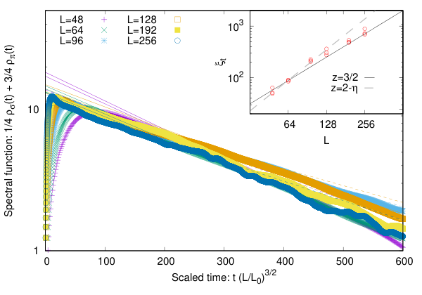
for an infinite system. Different curves in the left panel of Fig. 13 indicate power law fits, employing the values and for the dynamical critical exponent. We find that our results for the spectral function at zero spatial momentum favor the value of the so called “conventional theory" of dynamic critical phenomena, which emerges when the critical divergencies of kinetic coefficients is not taken into account in the scaling analysis RevModPhys.49.435. In fact this observation may be reinforced further by looking at the behavior of the spectral function in the time domain, where values of would lead to an increase of the spectral function function as a function at late times, which is clearly not observed in our simulations. Conversely, a value of (or ) would lead to a logarithmic time dependence (or power law decay) of the spectral function , which appears to be more consistent with our results.
It is also evident from Fig. 13, that for any finite-size system the critical behavior of the spectral function is suppressed by the exponential decay with the auto-correlation time . While for any finite system the auto-correlation time is finite, it diverges with increasing system size as , corresponding to the well known phenomenon of critical slowing down, and the typical way to extract the dynamical critical exponent in Monte-Carlo simulations. Our results for the analysis of the auto correlation time are compactly summarized in Fig. 14, where we we present fits to the late time exponential behavior of the spectral function along with the results for shown in the inset. While for small volumes the scaling of the auto-correlation time appears to be consistent with the predicted by the conventional theory, the behavior of for large volumes hints at a weaker divergence of the auto-correlation time consistent with on the larger lattices, as indicated by the solid and dashed curves in the inset of Fig. 14.
Since the frequency dependence of the critical spectral function , and the finite-size scaling of the auto-correlation time lead to different extractions of the dynamic critical exponent , we are unable to determine the dynamical critical behavior precisely from our current simulations. One possible explanation of the observed discrepancies could be due to the fact that we have set the spatial momentum prior to taking the limit (or ), which may or may not affect the critical scaling of the spectral function. In any case, it would be interesting to investigate the critical dynamics in more detail as a function of and at non-vanishing and , to further elucidate on the structure of excitations in the vicinity of the critical point. However, this will require significant computational resources and is well beyond the scope of our present work.
6 Conclusions
We have performed a detailed study of classical-statistical spectral functions in the relativistic model. While the static critical behavior is naturally reproduced correctly within the classical-statistical lattice approach, the focus of our study has been on the behavior of the real-time spectral functions and . While at very low temperatures, the classical-statistical approximation is inadequate and effectively reduces to a mean-field approximation, we argued that a classical-statistical description becomes accurate in the vicinity of a second order phase transition and demonstrated some intriguing features of the spectral functions close to the crossover transition and in the vicinity of the critical point.
In the broader context of non-perturbative calculations of real-time spectral functions, the results from classical-statistical simulations reported in this paper may provide additional guidance to alternative theoretical approaches, based, e.g. on functional methods or analytic continuation of Euclidean correlation functions, where prior information on the structure of excitations is required to devise suitable ansätze or efficient truncation schemes. Specifically, there is an interesting possibility to benchmark the quality of results obtained within functional approaches, based on a direct comparison of the results obtained in the classical-statistical limit. This is work in progress and will be reported elsewhere.
Acknowledgements
This research was supported by the Helmholtz International Center (HIC) for FAIR within the LOEWE initiative of the State of Hesse, and by the Deutsche Forschungsgemeinschaft (DFG) through the grant CRC-TR 211 “Strong-interaction matter under extreme conditions.”
References
- [1] G. D. Moore, O. Saremi, Journal of High Energy Physics 2008 (09) (2008) 015. doi:10.1088/1126-6708/2008/09/015.
- [2] J. Berges, S. Schlichting, D. Sexty, Nucl. Phys. B832 (2010) 228–240. arXiv:0912.3135, doi:10.1016/j.nuclphysb.2010.02.007.
- [3] M. Jarrell, J. Gubernatis, Physics Reports 269 (3) (1996) 133 – 195. doi:10.1016/0370-1573(95)00074-7.
- [4] M. Asakawa, Y. Nakahara, T. Hatsuda, Progress in Particle and Nuclear Physics 46 (2) (2001) 459 – 508. doi:10.1016/S0146-6410(01)00150-8.
- [5] Y. Burnier, A. Rothkopf, Phys. Rev. Lett. 111 (2013) 182003. doi:10.1103/PhysRevLett.111.182003.
- [6] B. B. Brandt, A. Francis, H. B. Meyer, D. Robaina, Phys. Rev. D 92 (2015) 094510. doi:10.1103/PhysRevD.92.094510.
- [7] L. Schlessinger, Phys. Rev. 167 (1968) 1411–1423. doi:10.1103/PhysRev.167.1411.
- [8] R.-A. Tripolt, I. Haritan, J. Wambach, N. Moiseyev, Physics Letters B 774 (2017) 411 – 416. doi:10.1016/j.physletb.2017.10.001.
- [9] D. Dudal, O. Oliveira, P. J. Silva, Phys. Rev. D 89 (2014) 014010. doi:10.1103/PhysRevD.89.014010.
- [10] R.-A. Tripolt, P. Gubler, M. Ulybyshev, L. Von Smekal, Comput. Phys. Commun. 237 (2019) 129–142. arXiv:1801.10348, doi:10.1016/j.cpc.2018.11.012.
- [11] J. Engels, O. Vogt, Nucl. Phys. B832 (2010) 538–566. arXiv:0911.1939, doi:10.1016/j.nuclphysb.2010.02.006.
- [12] D. Roeder, J. Ruppert, D. H. Rischke, Nucl. Phys. A775 (2006) 127–151. arXiv:hep-ph/0503042, doi:10.1016/j.nuclphysa.2006.05.007.
- [13] K. Kamikado, N. Strodthoff, L. von Smekal, J. Wambach, Eur. Phys. J. C74 (3) (2014) 2806. arXiv:1302.6199, doi:10.1140/epjc/s10052-014-2806-6.
- [14] R.-A. Tripolt, N. Strodthoff, L. von Smekal, J. Wambach, Phys. Rev. D89 (3) (2014) 034010. arXiv:1311.0630, doi:10.1103/PhysRevD.89.034010.
- [15] R.-A. Tripolt, L. von Smekal, J. Wambach, Phys. Rev. D90 (7) (2014) 074031. arXiv:1408.3512, doi:10.1103/PhysRevD.90.074031.
- [16] D. Mesterhazy, J. H. Stockemer, Y. Tanizaki, Phys. Rev. D92 (7) (2015) 076001. arXiv:1504.07268, doi:10.1103/PhysRevD.92.076001.
- [17] J. M. Pawlowski, N. Strodthoff, Phys. Rev. D92 (9) (2015) 094009. arXiv:1508.01160, doi:10.1103/PhysRevD.92.094009.
- [18] N. Strodthoff, Phys. Rev. D95 (7) (2017) 076002. arXiv:1611.05036, doi:10.1103/PhysRevD.95.076002.
- [19] J. M. Pawlowski, N. Strodthoff, N. Wink, Phys. Rev. D98 (7) (2018) 074008. arXiv:1711.07444, doi:10.1103/PhysRevD.98.074008.
- [20] J. A. Mueller, C. S. Fischer, D. Nickel, Eur. Phys. J. C70 (2010) 1037–1049. arXiv:1009.3762, doi:10.1140/epjc/s10052-010-1499-8.
- [21] C. S. Fischer, J. M. Pawlowski, A. Rothkopf, C. A. Welzbacher, Phys. Rev. D98 (1) (2018) 014009. arXiv:1705.03207, doi:10.1103/PhysRevD.98.014009.
- [22] G. Aarts, J. Smit, Nucl. Phys. B511 (1998) 451–478. arXiv:hep-ph/9707342, doi:10.1016/S0550-3213(97)00723-2.
- [23] R. Kubo, Journal of the Physical Society of Japan 12 (6) (1957) 570–586. doi:10.1143/JPSJ.12.570.
- [24] P. C. Martin, J. Schwinger, Phys. Rev. 115 (1959) 1342–1373. doi:10.1103/PhysRev.115.1342.
- [25] G. Aarts, Phys. Lett. B518 (2001) 315–322. arXiv:hep-ph/0108125, doi:10.1016/S0370-2693(01)01081-4.
- [26] P. C. Hohenberg, B. I. Halperin, Rev. Mod. Phys. 49 (1977) 435–479. doi:10.1103/RevModPhys.49.435.
- [27] R. D. Pisarski, F. Wilczek, Phys. Rev. D 29 (1984) 338–341. doi:10.1103/PhysRevD.29.338.
- [28] F. Wilczek, International Journal of Modern Physics A 07 (16) (1992) 3911–3925. doi:10.1142/S0217751X92001757.
- [29] K. Rajagopal, F. Wilczek, Nuclear Physics B 399 (2) (1993) 395 – 425. doi:10.1016/0550-3213(93)90502-G.
- [30] A. Polyakov, Physics Letters B 59 (1) (1975) 79 – 81. doi:10.1016/0370-2693(75)90161-6.
- [31] V. Novikov, M. Shifman, A. Vainshtein, V. Zakharov, Physics Reports 116 (3) (1984) 103 – 171. doi:10.1016/0370-1573(84)90021-8.
- [32] J. O. Andersen, D. Boer, H. J. Warringa, Phys. Rev. D69 (2004) 076006. arXiv:hep-ph/0309091, doi:10.1103/PhysRevD.69.076006.
- [33] E. Seel, D. Smith, S. Lottini, F. Giacosa, JHEP 07 (2013) 010. arXiv:1209.4243, doi:10.1007/JHEP07(2013)010.
- [34] G. Parisi, Statistical Field Theory, Addison-Wesley (Frontiers in Physics 66), 1988.
- [35] J. Berges, AIP Conf. Proc. 739 (2005) 3–62. arXiv:hep-ph/0409233, doi:10.1063/1.1843591.
- [36] A. Piñeiro Orioli, J. Berges, Phys. Rev. Lett. 122 (15) (2019) 150401. arXiv:1810.12392, doi:10.1103/PhysRevLett.122.150401.
- [37] M. Hasenbusch, T. Torok, J. Phys. A32 (1999) 6361. arXiv:cond-mat/9904408, doi:10.1088/0305-4470/32/36/301.
- [38] K. Kanaya, S. Kaya, Phys. Rev. D 51 (1995) 2404–2410. doi:10.1103/PhysRevD.51.2404.
- [39] J. Engels, T. Mendes, Nucl. Phys. B572 (2000) 289–304. arXiv:hep-lat/9911028, doi:10.1016/S0550-3213(00)00046-8.
- [40] A. Pelissetto, E. Vicari, Phys. Rept. 368 (2002) 549–727. arXiv:cond-mat/0012164, doi:10.1016/S0370-1573(02)00219-3.
- [41] J. Engels, S. Holtmann, T. Mendes, T. Schulze, Physics Letters B 514 (3) (2001) 299 – 308. doi:10.1016/S0370-2693(01)00798-5.
- [42] J. Engels, L. Fromme, M. Seniuch, Nucl. Phys. B675 (2003) 533–554. arXiv:hep-lat/0307032, doi:10.1016/j.nuclphysb.2003.09.060.
- [43] J. Engels, F. Karsch, Phys. Rev. D90 (1) (2014) 014501. arXiv:1402.5302, doi:10.1103/PhysRevD.90.014501.
- [44] A. M. Ferrenberg, R. H. Swendsen, Phys. Rev. Lett. 61 (1988) 2635–2638. doi:10.1103/PhysRevLett.61.2635.
- [45] P. Springer, Finite Volume Effects and the Binder Cumulant in -Model, M.Sc. Thesis, Technische Universiät München, 2013.
- [46] B. I. Halperin, P. C. Hohenberg, S.-k. Ma, Phys. Rev. B10 (1974) 139–153. doi:10.1103/PhysRevB.10.139.
- [47] K. Rajagopal, F. Wilczek, Nucl. Phys. B399 (1993) 395–425. arXiv:hep-ph/9210253, doi:10.1016/0550-3213(93)90502-G.