Space-adaptive anisotropic bivariate Laplacian regularization for image restoration

Image restoration is the task of recovering a sharp image $u$ starting from a blurred and noisy observation $g$. In this work, we consider a degradation model of the form

$$g=Ku+e\,,$$

(2)

where $g,u\in\mathbb{R}^{n}$ are vectorized images, $K\in\mathbb{R}^{n\times n}$ is the linear blur operator and $e\in\mathbb{R}^{n}$ is an additive noise vector. A possible strategy to overcome the ill-posedeness of the linear system in (2) is to reformulate the problem. We thus look for $u^{*}$, estimate of the original $u$, which solves a well-posed problem. In the variational approach, $u^{*}$ is the minimizer of a cost functional $\mathcal{J}(u;K,g):\mathbb{R}^{n}\to\mathbb{R}$. In formula,

$$u^{*}\in\arg\min_{u\in\mathbb{R}^{n}}\;\big\{\mathcal{J}(u;K,g):=\mathcal{R}(u)+\mu\mathcal{F}(u;K,g)\big\}.$$

(3)

The functionals $\mathcal{R}$ and $\mathcal{F}$ are commonly referred to as the regularization and the data fidelity term, respectively. While $\mathcal{R}$ encodes prior information on the desired image $u$, $\mathcal{F}$ is a data term which measures the ‘distance’ between the given image $g$ and $u$ after the action of the operator $K$ with respect to some norm corresponding to the noise statistics in the data, cf., e.g., stuart. The regularization parameter $\mu>0$ controls the trade-off between the two terms.
In this paper, we consider an Additive White Gaussian Noise (AWGN) corrupting the blurred image $Ku$, i.e. $e\sim\mathcal{N}(0,\sigma^{2}I_{n})$, where $I_{n}$ is the $n$-dimensional identity matrix. It is well known that, in presence of AWGN, a suitable choice for $\mathcal{F}(u;K,g)$ is the so-called L₂ fidelity term, reading as,

$$\mathcal{F}(u;K,g)=\mathrm{L}_{2}(u;K,g)=\frac{1}{2}\lVert Ku-g\rVert_{2}^{2}.$$

(4)

A popular choice for the regularization term $\mathcal{R}(u)$ is given by the TV semi-norm ROF,

$$\mathcal{R}(u)=\mathrm{TV}(u)=\sum_{i=1}^{n}\lVert(\nabla u)_{i}\rVert_{2}\,,$$

(5)

where $(\nabla u)_{i}:=\big((D_{h}u)_{i},(D_{v}u)_{i}\big)^{T}\in\mathbb{R}^{2}$ denotes the discrete gradient of image $u$ at pixel $i$, with $D_{h},D_{v}\in\mathbb{R}^{n\times n}$ linear operators representing finite difference discretizations of the first-order horizontal and vertical partial derivatives, respectively.
Coupling the L₂ data term with the TV regularizer leads to one of the most widespread variational models for image restoration problem, the TV-L₂ (or ROF) model,

$$u^{*}\in\arg\min_{u\in\mathbb{R}^{n}}\bigg\{\sum_{i=1}^{n}\lVert(\nabla u)_{i}\rVert_{2}+\frac{\mu}{2}\lVert Ku-g\rVert_{2}^{2}\bigg\}.$$

(6)

The global perspective of the TV-L₂ model does not allow to diversify the action of the regularizer on regions of the image presenting different properties. In siam; ncmip; cmbbe; vip, the authors have proposed space-variant regularization term based on statistical assumptions on the distribution of the $\ell_{2}$-norm of the gradients and on the gradients themselves.
In this paper, we propose a space-variant anisotropic extension of the TV regularizer in (5) which, as it will be illustrated in Sect. 2, comes from the a priori assumption that the gradients of the target image $u$ distribute locally according to a Bivariate Laplace Distribution (BLD). The proposed BLTV regularizer takes the form

	$\displaystyle\mathrm{BLTV}(u;\lambda_{1},\lambda_{2},\theta)$	$\displaystyle=$	$\displaystyle\sum_{i=1}^{n}\lVert\Lambda_{i}R_{\theta_{i}}(\nabla u)_{i}\rVert_{1}$		(7)
		$\displaystyle=$	$\displaystyle\sum_{i=1}^{n}\bigg[\lambda_{i}^{(1)}|\langle r_{i}^{(1)},(\nabla u)_{i}\rangle|+\lambda_{i}^{(2)}|\langle r_{i}^{(2)},(\nabla u)_{i}\rangle|\bigg]\,,$		(8)

where $\Lambda_{i}$ is a $2\times 2$ positive definite diagonal matrix and $R_{\theta_{i}}$ is the rotation matrix corresponding to the angle $-\theta_{i}$. Mathematically,

$$\Lambda_{i}=\begin{pmatrix}\lambda_{i}^{(1)}&0\\ 0&\lambda_{i}^{(2)}\end{pmatrix}\,,\quad R_{\theta_{i}}=\begin{pmatrix}\cos\theta_{i}&\sin\theta_{i}\\ -\sin\theta_{i}&\cos\theta_{i}\end{pmatrix}=\begin{pmatrix}r_{i}^{(1)}\\ r_{i}^{(2)}\end{pmatrix}.$$

(9)

We denote by $\lambda_{1},\lambda_{2},\theta\in\mathbb{R}^{n}$ the maps of the parameters defining the local distributions. Hence, the proposed BLTV-L₂ variational restoration model reads as

$$u^{*}\in\arg\min_{u\in\mathbb{R}^{n}}\bigg\{\mathrm{BLTV}(u;\lambda_{1},\lambda_{2},\theta)+\frac{\mu}{2}\lVert Ku-g\rVert_{2}^{2}\bigg\}.$$

(10)

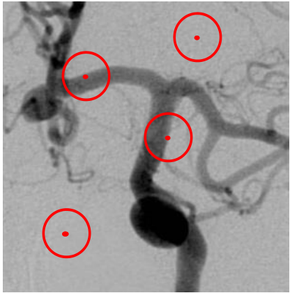
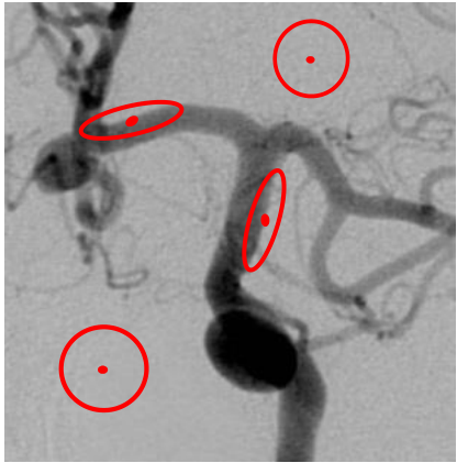
The $3n$ free parameters defining the BLTV regularizer in (7)–(9) hold the potential for effectively modelling local image properties, in particular driving in a suitable adaptive manner the strength and direction of non-linear TV-diffusion. In Figs.1(a)-(b) the red ellipses represent TV-diffusion strengths along all possible directions at few sample pixel locations for TV and BLTV regularizers. It is evident how for classical TV such ellipses turn out to be circles (isotropy) of constant radius (space-invariance), whereas our BLTV regularizer allows for ellipses (anistropy) of different size (space-variance). In practice, such flexibility of BLTV can be (and will be) exploited to diffuse in different ways in regions exhibiting different properties: for instance, strong isotropic diffusion in homogeneous regions, strongly anisotropic diffusion in regions characterized by a dominant edge direction. In Figs.1 (c)-(d) we show the level curves of the TV regularizer and one among the infinity of possible configuration of the level curves of the BLTV regularizer, respectively, revealing once again the flexibility of the proposed regularizer.

Together with the variational model in (10), we also propose an efficient and robust procedure for automatically estimating the parameter maps $\lambda^{(1)}$, $\lambda^{(2)}$, $\theta$ based on a Maximum Likelihood (ML) approach. The parameter maps can be updated along the iterations of the Alternating Direction Methods of Multipliers (ADMM), which is the algorithm adopted here to solve the minimization problem. Notice that the convexity of the BLTV-L₂ model ensures the convergence of the ADMM.

Applying the Maximum A Posteriori (MAP) estimation approach to image restoration consists in computing the restored image as a global maximizer of the posterior probability Pr$(u|g;K)$ of the unknown target image $u$ given the observation $g$, namely:

$$u^{*}\>\;{\in}\;\>\arg\max_{u\in\mathbb{R}^{n}}\;\text{Pr}(u|g;K)=\arg\min_{u\in\mathbb{R}^{n}}\;\left\{\,-\mathrm{ln}\text{Pr}(g|u;K)-\mathrm{ln}\text{Pr}(u)\,\right\}\,,$$

(11)

where, after applying the Bayes’ rule, we drop the evidence term Pr$(g)$ and extracted $-\ln$ of the objective function. The two terms Pr$(u)$ and Pr$(g|u;K)$ in (11) are referred to as the prior and the likelihood. The likelihood term associated with AWGN corruption takes the form

$$\mathrm{Pr}(g|u;K)=\prod_{i=1}^{n}\,\frac{1}{\sqrt{2\pi}\sigma}\,\text{exp}\bigg(-\frac{(Ku-g)_{i}^{2}}{2\sigma^{2}}\,\bigg)=W\,\text{exp}\bigg(-\frac{\lVert Ku-g\rVert_{2}^{2}}{2\sigma^{2}}\,\bigg),$$

(12)

where $\sigma>0$ denotes the AWGN standard deviation and $W>0$ is a normalization constant. For what concerns the prior, a common choice is to model the unknown image $u$ as a Markov Random Field (MRF) such that the image can be characterized by its Gibbs prior distribution, whose general form is:

$$\text{Pr}(u)=\prod_{i=1}^{n}\text{Pr}_{i}(u)=\prod_{i=1}^{n}z_{i}\,\text{exp}\,(\,-\alpha\,V_{c_{i}}(u)\,)=Z\,\text{exp}\,\bigg(\,-\alpha\,\sum_{i=1}^{n}V_{c_{i}}(u)\,\bigg),$$

(13)

where $\alpha>0$ is the MRF parameter, $\{c_{i}\}_{i=1}^{n}$ is the set of all cliques (a clique is a set of neighboring pixels) for the MRF, $V_{c_{i}}$ is the potential function defined on the clique $c_{i}$ and $Z=\prod_{i=1}^{n}z_{i}$ is a normalization constant. Choosing as potential function at the generic $i$-th pixel the magnitude of the discrete gradient at the same pixel, i.e. $V_{c_{i}}=\lVert(\nabla u)_{i}\rVert_{2}$ for any $i\in\{1,\ldots,n\}$, the Gibbs prior in (13) reduces to the TV prior which, plugged into (11), yields the popular TV regularizer. We remark that the TV prior corresponds to choosing

$$\text{Pr}_{i}(u)=z_{i}\,\text{exp}\,\left(\,-\alpha\lVert(\nabla u)_{i}\rVert_{2}\right)\,.$$

(14)

Here, we propose a space-variant anisotropic generalization of the local prior $\text{Pr}_{i}(u)$ above. More in detail, we assume that the discrete gradient at any pixel $i$ distributes according to a space-variant BLD, such that our prior reads as

	$\displaystyle\mathrm{Pr}(u)$	$\displaystyle=$	$\displaystyle\prod_{i=1}^{n}\text{Pr}_{i}(u)=\prod_{i=1}^{n}z_{i}\,\exp\bigg(-\lVert\Lambda_{i}R_{\theta_{i}}(\nabla u)_{i}\rVert_{1}\bigg)$		(15)
		$\displaystyle=$	$\displaystyle Z\,\exp\bigg(-\sum_{i=1}^{n}\lVert\Lambda_{i}R_{\theta_{i}}(\nabla u)_{i}\rVert_{1}\bigg)\,,$

where $Z$ is the normalization constant and $\Lambda_{i},R_{{\theta}_{i}}\in\mathbb{R}^{2\times 2}$ are defined in (9).

Plugging the prior (15) and the likelihood (12) into (11) and neglecting the constant terms, the proposed BLTV-L₂ variational model (10) is obtained.

In order to make the introduction of the proposed regularizer actually useful, an efficient, robust, and automatic procedure for the estimation of the parameter maps $\lambda^{(1)},\lambda^{(2)},\theta\in\mathbb{R}^{n}$ identifying all the local BLDs has to be proposed as well. To this aim, we resort to the ML approach. Consider a set of $N$ 2-dimensional samples $\mathcal{S}:=\left\{s_{1},\ldots,s_{N}\right\}$ drawn from a BLD with parameters $(\lambda_{1},\lambda_{2},\theta)$. Here, the samples play the role of image gradients at pixels of a neighborhood of radius $r$ centered at a generic pixel $i$. Assuming independence of the samples, according to the definition of BLD, the likelihood function is defined by

$$\mathrm{Pr}(\mathcal{S}|\lambda_{1},\lambda_{2},\theta)=\bigg(\frac{\lambda_{1}\,\lambda_{2}}{4}\bigg)^{N}\exp\bigg(-\sum_{i=1}^{N}\bigg(\lambda_{1}|\langle r_{1},s_{i}\rangle|+\lambda_{2}|\langle r_{2},s_{i}\rangle|\bigg)\bigg)\,,$$

(16)

where, clearly, $r_{1}$ and $r_{2}$ depend on $\theta$ - see (9). The goal here is to find

	$\displaystyle(\lambda_{1}^{*},\lambda_{2}^{*},\theta^{*})$	$\displaystyle\in$	$\displaystyle\arg\max_{\lambda_{1},\lambda_{2},\theta}\mathrm{Pr}(\mathcal{S}|\lambda_{1},\lambda_{2},\theta)=\arg\min_{\lambda_{1},\lambda_{2},\theta}-\mathrm{ln}\mathrm{Pr}(\mathcal{S}|\lambda_{1},\lambda_{2},\theta)$		(17)
		$\displaystyle=$	$\displaystyle-N\mathrm{ln}\frac{\lambda_{1}\,\lambda_{2}}{4}+\sum_{i=1}^{N}\bigg(\lambda_{1}|\langle r_{1},s_{i}\rangle|+\lambda_{2}|\langle r_{2},s_{i}\rangle|\bigg).$

Imposing a first-order optimality condition with respect to $\lambda_{1},\lambda_{2}$ leads to the following closed-form estimation formulas:

$$\lambda_{1}=\bigg(\frac{1}{N}\sum_{i=1}^{N}|\langle r_{1},s_{i}\rangle|\bigg)^{-1}\,,\quad\lambda_{2}=\bigg(\frac{1}{N}\sum_{i=1}^{N}|\langle r_{2},s_{i}\rangle|\bigg)^{-1}.$$

(18)

Substituting the expressions in (18) into the objective function (17), we thus obtain the simplified minimization problem in the only variable $\theta$:

$$\theta^{*}\in\arg\min_{\theta}\bigg\{\mathrm{ln}\bigg(\sum_{i=1}^{N}|\langle r_{1},s_{i}\rangle|\bigg)+\mathrm{ln}\bigg(\sum_{i=1}^{N}|\langle r_{2},s_{i}\rangle|\bigg)\bigg\}\,.$$

(19)

In order to solve numerically the proposed image restoration model (10), we use an ADMM-based algorithm - see boyd. We first introduce two auxiliary variables $w\in\mathbb{R}^{n}$, $t\in\mathbb{R}^{2n}$ and rewrite the model in the equivalent linearly constrained form:

	$\displaystyle\{\,u^{*},w^{*},t^{*}\}$	$\displaystyle\>\;{\in}\;\>$	$\displaystyle\arg\min_{u,w,t}\bigg\{\>\sum_{i=1}^{n}\lVert\Lambda_{i}R_{\theta_{i}}t_{i}\rVert_{1}\;{+}\;\frac{\mu}{2}\,\|w\|_{2}^{2}\>\bigg\}$		(21)
			$\displaystyle\mathrm{subject}\;\mathrm{to}:\quad w\;{=}\;Ku-g,\;\>t\;{=}\;Du,$

where the space-variant matrices $\Lambda_{i}$, $R_{\theta_{i}}$ can be estimated via the ML procedure described in Sect. 3 based only on the observed image $g$ (i.e. as a preliminary pre-processing step) or also updated along the ADMM iterations. We define the augmented Lagrangian functional:

	$\displaystyle\mathcal{L}(u,w,t;\rho_{w},\rho_{t})$	$\displaystyle:=$	$\displaystyle\sum_{i=1}^{n}\lVert\Lambda_{i}R_{\theta_{i}}t_{i}\rVert_{1}+\frac{\mu}{2}\|w\|_{2}^{2}-\rho_{t}^{T}(t-Du)+\frac{\beta_{t}}{2}\|t-Du\|_{2}^{2}$		(22)
		$\displaystyle-$	$\displaystyle\rho_{w}^{T}(w-(Ku-g))+\frac{\beta_{w}}{2}\|w-(Ku-g)\|_{2}^{2},$

where $\beta_{w},\beta_{t}>0$ are scalar penalty parameters and $\rho_{w}\in\mathbb{R}^{n}$, $\rho_{t}\in\mathbb{R}^{2n}$ are the vectors of Lagrange multipliers associated with the given linear constraints. The solution $\{u^{*},w^{*},t^{*}\}$ of problem (21) is a saddle point for $\mathcal{L}$ in (22), see, e.g., boyd. Hence, we can alternate a minimization step with respect to $t,u,w$ with a maximization step with respect to $\rho_{t},\rho_{w}$. Mathematically,

		$\displaystyle u^{(k+1)}$	$\displaystyle\;{\leftarrow}\;\;\,\,\arg\min_{u\in\mathbb{R}^{n}}\;\mathcal{L}(u,w^{(k)},t^{(k)};\rho_{w}^{(k)},\rho_{t}^{(k)})\,,$		(23)
		$\displaystyle w^{(k+1)}$	$\displaystyle\;{\leftarrow}\;\;\,\,\arg\min_{r\in\mathbb{R}^{n}}\;\mathcal{L}(u^{(k+1)},w,t^{(k)};\rho_{w}^{(k)},\rho_{t}^{(k)})\,,$		(24)
		$\displaystyle t^{(k+1)}$	$\displaystyle\;{\leftarrow}\;\;\,\,\arg\min_{t\in\mathbb{R}^{2n}}\;\mathcal{L}(u^{(k+1)},w^{(k+1)},t;\rho_{w}^{(k)},\rho_{t}^{(k)})\,,$		(25)
		$\displaystyle\rho_{w}^{(k+1)}$	$\displaystyle\;{\leftarrow}\;\;\,\,\rho_{w}^{(k)}\;{-}\;\beta_{r}\,\big(\,w^{(k+1)}\;{-}\;(Ku^{(k+1)}-g)\,\big)\,,$		(26)
		$\displaystyle\rho_{t}^{(k+1)}$	$\displaystyle\;{\leftarrow}\;\;\,\,\rho_{t}^{(k)}\;{-}\;\beta_{t}\,\big(\,t^{(k+1)}\;{-}\;Du^{(k+1)}\,\big)\,.$		(27)

In this section, we evaluate the performance of the proposed BLTV-L₂ restoration model compared with the baseline TV-L₂ model, also solved by ADMM. The stopping criteria of the ADMM for both models are defined based on the number of iterations as well as on the iterates relative change, i.e. we stop iterating as soon as

$$k\geq 1500\;\;\;\mathrm{or}\;\;\;\delta^{(k)}:=\frac{\lVert u^{(k)}-u^{(k-1)}\rVert}{\lVert u^{(k-1)}\rVert}\geq 10^{-6}.$$

(28)

The quality of the restored images $u^{*}$ is measured by means of the Improved Signal-to-Noise Ratio $\mathrm{ISNR}(u^{*},g,u)=10\log_{10}\frac{\|g-u\|_{2}^{2}}{\|u^{*}-u\|_{2}^{2}}$, with $u$ denoting the original uncorrupted image, and of the Structural-Similarity-Index (SSIM) ssim.

We consider the test image brain in Fig.2 (a) (570 $\times$ 430) and the test image abdomen in Fig.4 (a) (350 $\times$ 480) with pixel values between 0 and 255, synthetically corrupted by space-invariant blur with Gaussian kernel of parameters band = 9, sigma = 2, and by AWGN of different levels $\sigma\in\{10,20\}$ - see, e.g., Fig.2 (b) and Fig.4 (b). The parameter maps are computed at the beginning starting from the observed image $g$ and then updated every 300 iterations based on the current iterate. The radius of the neighborhoods used for the local parameter estimation has been set equal to 8 and 5 for the brain and abdomen test images, respectively. The reconstructions of brain for $\sigma=20$ and of abdomen for $\sigma=10$ via TV-L₂ and BLTV-L₂ models are shown in Figs.2(c)-(d) and Figs.4(c)-(d), respectively.

From a visual inspection, the restoration via BLTV-L₂ seems to be more neat and less cartooned than the TV reconstructions. As reported in Tab.1, the ISNR and SSIM values for the two test images and for different noise levels obtained by the BLTV-L₂ model outperform the ones reached by the TV-L₂ model.
The final parameter maps computed by BLTV-L₂ are shown in Figs. 3-5.

Computational times. We tested the joint parameter estimation + reconstruction model on a standard laptop with inbuilt MATLAB software, version 2016b. As far as the ML parameter estimation of the parameter maps procedure is concerned, we notice that the update (18) is explicit, thus very cheap, whereas the computation of $\theta^{*}$ in (19) requires the solution of an optimisation problem. We solve the problem by line-searching upon a suitable discretization of the parameter space. For Fig. 2, the ML parameter estimation procedure took 8.45 secs.

The ADMM algorithmic sub-steps with automatic parameter update every 300 iterations computes the numerical solution in 381 secs for the high-resolution image in Fig. 2. A possible way to accelerate the speed of the algorithm would be the computation the parameter maps only in terms of the given image and not along the iterations, although of course that would render a less accurate result.

We presented a new space-variant anisotropic regularization term for image restoration based on the a priori statistical assumption that the gradients of the unknown target image distribute locally according to space-variant bivariate Laplace distributions. The high flexibility of the proposed regularizer together with the presented ML parameters estimation procedure and ADMM-based minimization algorithm yield a very effective and efficient approach. Preliminary experiments on images corrupted by blur and AWGN strongly indicate that the proposed variational model achieves high-quality restorations and, in particular, outperforms by far the results obtained by classical TV-regularized restoration models. Coupling the proposed regularizer with other fidelity terms suitable for dealing with noises other than Gaussian - such as, e.g., Laplace, Poisson and mixed Poisson-Gaussian MIXED - is a matter being studied.

References

- (1) Boyd, S., Parikh, N., Chu, E., Peleato, B., Eckstein, J.: Distributed optimization and statistical learning via the alternating direction method of multipliers: In: Foundations and Trends in Machine Learning, 3 (2011).
- (2) Calatroni, L., Lanza, A., Pragliola, M., Sgallari, F.: A flexible space-variant anisotropic regularisation for image restoration with automated parameter selection. In: SIAM Journal of Imaging Sciences, 12 (2019).
- (3) Calatroni, L., Lanza, A., Pragliola, M., Sgallari, F.: Adaptive parameter selection for weighted-TV image reconstruction problems. In: Journal of Physics: Conference Series, NCMIP 2019, to appear (2019).
- (4) He, C., Hu, C., Zhang, W. and Shi, B.: A Fast Adaptive Parameter Estimation for Total Variation Image Restoration. In: IEEE Transactions on Image Processing, 23 (2014).
- (5) Lanza, A., Morigi, S., Pragliola, M., Sgallari, F.: Space-variant generalised gaussian regularisation for image restoration. In: Computational Methods in Biomechanics and Biomedical Engineering: Imaging and Visualization, 13 (2018).
- (6) Lanza, A., Morigi, S., Pragliola, M., Sgallari, F.: Space-variant TV regularization for image restoration. In: VipIMAGE 2017, J. M. R. Tavares and R. Natal Jorge, eds., Cham, Springer International Publishing, (2018).
- (7) Lanza, A., Morigi, S., Sgallari, F.: Constrained TVp- model for image restoration. In: Journal of Scientific Computing, 68 (2016).
- (8) Lanza, A., Morigi, S., Sgallari, F., Wen, Y.W.: Image restoration with Poisson - Gaussian mixed noise. In: Computer Methods in Biomechanics and Biomedical Engineering: Imaging & Visualization, 2 (2014).
- (9) Rudin, L.I., Osher, S., Fatemi, E.: Nonlinear total variation based noise removal algorithms. In: Physica D: Nonlinear Phenomena, 60 (1992).
- (10) Stuart, A.M.: Inverse problems: a Bayesian perspective. In: Acta Numerica, 19 (2010).
- (11) Zhou, W., Bovik, A., Sheikh, H., Simoncelli, E.: Image quality assessment: From error visibility to structural similarity. In: IEEE Transactions on Image Processing, 13 (2004).