跳到论文正文
W Papers独立论文阅读器 arXiv:1908.00705 论文正文 计算阅读时间 · 0%
引用这篇论文根据当前论文元数据生成,正式投稿前建议核对。


License: arXiv.org perpetual non-exclusive license
arXiv:1908.00705v1 [quant-ph] 02 Aug 2019

Asymmetric quantum multicast network coding: asymmetric optimal cloning over quantum networks

Yuichi Hirota Affiliation: 1 Department of Computer Science, Faculty of Informatics, Shizuoka University
3-5-1 Johoku, Naka-ku, Hamamatsu 432-8011, JAPAN
   Masaki Owari Affiliation: 1 Department of Computer Science, Faculty of Informatics, Shizuoka University
3-5-1 Johoku, Naka-ku, Hamamatsu 432-8011, JAPAN
Abstract

In this study, we consider a quantum version of multicast network coding as a multicast protocol for sending universal quantum clones (UQCs) from a source node to the target nodes on a quantum network. By extending Owari et al.’s previous results for symmetric UQCs, we derive a protocol for multicasting 1→21\rightarrow 2 (1→31\rightarrow 3) asymmetric UQCs of a qrq^{r}-dimensional state to two (three) target nodes. Our protocol works under the condition that each edge on a quantum network represented by an undirected graph GG transmits a qq-dimensional state. There exists a classical solvable linear multicast network code with a source rate of rr on a classical network G′G^{\prime}, where GG is an undirected underlying graph of an acyclic directed graph G′G^{\prime}. We also assume free classical communication over a quantum network.

I Introduction

The throughput of a network can be improved by applying non-trivial operations to the bitstream at intermediate nodes when there is a bottleneck on a network HL08; Y08. This protocol can be referred to as network coding. The network coding research was started in classical information theory ACLY00. The network coding for a quantum network is called “quantum network coding” HINRY07. There has been a considerable amount of research on quantum network coding, which can improve the throughput of a quantum network in various situations Hayashi07; Shi06; Kobayashi09; Kobayashi10; Leung10; Kobayashi11; OKM13; KOM14; KOM15; EKB16. Recently, it has been presented that quantum network coding can improve the security of a quantum network OKH17a; OKH17b; SH18a; SH18b. Further, it is useful for quantum repeater networks SINV16; MSNV18 as well as for distributed quantum computationAM16. Although many studies have considered network coding on noisy classical networks, almost all the studies of quantum network coding consider noise-free quantum networks. This is because quantum network coding is regarded as a protocol implemented on a layer after the errors have already corrected. Hence, in this study, we consider noise-free quantum networks.

In classical network coding, majority of the studies have focused on multicast communication, where a single source node transmits the same information to multiple target nodes on a networkHL08; Y08. Figure 1 shows the network coding for a the butterfly network. This is one of the simplest examples of classical multicast network coding. Another type of network coding is called multiple-unicast network coding. Here, there are kk pairs of source and target nodes (s0,t0),…,(sk−1,tk−1)(s_{0},t_{0}),...,(s_{k-1},t_{k-1}) on the network, and each source node sis_{i} independently transmits a message to the corresponding target node tit_{i} for all iiTRLKM06. The modified version of the butterfly network in Figure 2 is one of the simplest examples of classical multiple-unicast network coding.

Most of the research on quantum network coding considered multiple-unicast communication, i.e., multiple-unicast quantum network coding. This differs from classical network coding because each source node transmits a quantum state (instead of a classical message) to the corresponding target nodeHayashi07; Kobayashi09; Leung10; Kobayashi11; EKB16; OKH17a; OKH17b; SH18a; SH18b; SINV16; MSNV18. The most important results are those of Kobayashi et al.. If classical information (or measurement results) can be freely sent among the nodes on a quantum network, Kobayashi et al. gave a canonical procedure for constructing a quantum multiple-unicast network code from a classical multiple-unicast network code. The quantum network for the quantum code and the classical network for the classical code must represented by the same graph Kobayashi09; Kobayashi11.

Refer to caption
Figure 1: Multicast classical network coding on the butterfly network. A single source node ss sends messages b0b_{0} and b1b_{1} on 𝔽p:=ℤ/ℤp\mathbb{F}_{p}:=\mathbb{Z}/\mathbb{Z}_{p} to both target nodes t1t_{1} and t2t_{2}.
Refer to caption
Figure 2: Multiple-unicast classical network coding on the butterfly network. A source node s0s_{0} sends message b0∈𝔽pb_{0}\in\mathbb{F}_{p} to target node t0t_{0}, and source node s1s_{1} sends message b1∈𝔽pb_{1}\in\mathbb{F}_{p} to target node t1t_{1}.

Unlike quantum multiple-unicast network coding, there has been less research on quantum network coding focusing on multicast communicationShi06; Kobayashi10; OKM13; KOM14; KOM15. This is because in quantum information theory, no-cloning theory prohibits perfect multicast communication WZ82, and, thus, it is not straightforward to construct a multicast quantum network coding protocol as an extension of a classical multicast network coding protocol.

Shi et al.’s paper is the first to treat quantum multicast network coding Shi06. They consider the problem of distributing NN-identical copies of a state |ψ⟩\left|\psi\right\rangle from a single source node to NN target nodes. Since the number of copies of |ψ⟩\left|\psi\right\rangle is equal to the number of nodes, |ψ⟩\left|\psi\right\rangle can be distributed without cloning the quantum states. Shi et al. showed that coding on intermediate nodes can increase the throughput of the quantum network. The second work treating this topic is Kobayashi et al.’s paper Kobayashi10. In this paper, a single copy of a state |ψ⟩=∑i=1dαi|i⟩\left|\psi\right\rangle=\sum_{i=1}^{d}\alpha_{i}\left|i\right\rangle is given on the source node and the aim is to share a Greenberger-Horne-Zeilinger (GHZ-)-type state ∑i=1dαi|i⟩1⊗⋯⊗|i⟩N\sum_{i=1}^{d}\alpha_{i}\left|i\right\rangle_{1}\otimes\cdots\otimes\left|i\right\rangle_{N} among target nodes, where the iith local system is on the iith target node. From this GHZ-type state between the target nodes, the input state |Ψ⟩\left|\Psi\right\rangle can be reconstructed at any target node by local operations and classical communication (LOCC). Based on classical multicast network coding, Kobayashi et al. developed a quantum protocol to achieve the above task under the assumption of free classical communication among nodes on the quantum network.

Although Shi et al.’s protocol and Kobayashi et al.’s protocol can be considered as generalizations of classical multicast network coding to quantum networks , rigorously speaking, the goal of their protocols is not exactly to achieve a multicast of a quantum state. Since an optimal multicast quantum channel is nothing but an optimal cloningBH96; SIG05; FWJYSZM14, a protocol to share an optimal clone of an input state among target nodes of a quantum network can be considered as one of the most natural quantum extensions of a multicast classical network coding protocol. Based on this idea, Owari et al. constructed a protocol to share a symmetric optimal universal clone of an input state on the target nodes under the conditions that classical information can be sent freely among nodes on a quantum network and that a small amount of entanglement is shared on target nodes at the beginning of the protocolOKM13; KOM14; KOM15.

In this paper, we focus on extending Owari et al.’s results to asymmetric optimal universal cloningNG98; C98; C00; IACFFG05, which is a generalization of symmetric optimal universal cloning. Thus, we construct a protocol to efficiently multicast an asymmetric optimal clone of a qrq^{r}-dimensional input quantum state from one source node to two (three) target nodes, where qq is assumed to be a prime power. In this protocol, the following five conditions are assumed:

  • •

    The noise free quantum network can be described by an undirected graph GG with one source node and two(three) target nodes.

  • •

    Each quantum channel on the quantum network can transmit one qq-dimensional quantum system in a single session.

  • •

    There exists a classical solvable linear multicast network code with source rate rr for a noise-free classical network described by an acyclic directed graph G′G^{\prime}, where GG is an undirected underlying graph of G′G^{\prime}.

  • •

    Measurement results (or classical information) can be sent freely from one node to another node on the quantum network.

  • •

    A small amount of entanglement which does not scale with qq, is shared among the target nodes. The amount of entanglement is at most 22 ebit for two target nodes, and at most (2+4​log2​3)\left(2+4\log_{2}3\right) ebit for the case of tree target nodes.

Using the max-flow and min-cut theorem of multicast network coding HL08; Y08, for sufficiently large qq, the assumption for the existence of a classical network code on G′G^{\prime} can be replaced by the condition that the minimum-cut between the source node ss and a target node tit_{i} is no less than rr for all ii.

An outline of our protocol is as follows:

  • •

    We creat two (three) asymmetric optimal clones of an input state with an ancilla system at a source node.

  • •

    We measure the ancilla system, and send the measurement outcomes to the target nodes.

  • •

    We compress the whole d2d^{2} (d3d^{3})-dimensional system into a dd-dimensional system.

  • •

    We transmit the resulting state to two(three) target nodes using Kobayashi et al.’s multicast quantum network codingKobayashi10. As a result, a GHZ-type state is shared among target nodes.

  • •

    We reconstruct the asymmetric clones of the input state from the GHZ-type state using LOCC with a small amount of entanglement among the target nodes and the measurement outcomes sent from the source node.

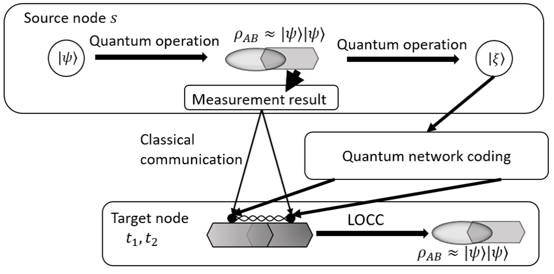
Using the above protocol, we can multicast asymmetric optimal clones from one source node to two(three) target nodes (Figure 3).
Refer to caption
Figure 3: Schematic diagram of a protocol for multicasting asymmetric optimal clones from one source node to two target nodes. The asymmetric optimal cloning protocol for the input state |ψ⟩\left|\psi\right\rangle is implemented at the source node.ng The resulti state is compressed into a dd-dimensional system, and transmitted to the two target nodes using Kobayashi et al.’s quantum multicast network coding protocol. Finally, the asymmetric clones of the input state are reconstructed by LOCC on target nodes with the help of a small amount of entanglement.

The rest of paper is organized as follows: We explain the asymmetric cloning and Kobayashi et al.’s quantum multicast network coding protocol in Section II. We present a procol for multicasting 1→21\rightarrow 2 asymmetric optimal clones in Section III. We also present a procol for multicasting 1→31\rightarrow 3 asymmetric optimal clones in Section IV. Finally, we gives an conclusion in Section V.

II Preliminaries

Optimal asymmetric universal quantum cloning, classical linear multicast network coding and Kobayashi et al.’s multicast quantum network coding protocol are all important in our protocol. In this section, we explain optimal asymmetric universal quantum cloning in Section II.1. Then, classical linear multicast network coding and the Kobayashi et al.’s multicast quantum network coding protocol are presented in Sections II.2 and II.3, respectively.

II.1 Optimal asymmetric quantum universal cloning machine

No-cloning theorem states that quantum mechanics prohibits a quantum operation that makes perfect copies of an unknown quantum stateWZ82. In other words, a perfect multicast of an unknown quantum state is impossible. On the other hand, quantum mechanics does not completely prohibit the approximate cloning of a quantum state. Hence, many studies have focused on quantum protocols to make an approximate copy of unknown states (so called quantum cloning machines) BH96; SIG05; FWJYSZM14; C00; IACFFG05.

A quantum cloning machine (QCM) that produces NN approximate clones based on MM copies of a given quantum state |ψ⟩∈ℋ\left|\psi\right\rangle\in\mathcal{H} is a quantum channel (or a completely positive and trace preserving map) ε\varepsilon from 𝔅⁡(ℋ⊗M)\mathfrak{B}\left(\mathcal{H}^{\otimes M}\right) to 𝔅⁡(ℋ⊗N)\mathfrak{B}\left(\mathcal{H}^{\otimes N}\right), where 𝔅⁡(ℋ)\mathfrak{B}\left(\mathcal{H}\right) is a space of all linear operators on the Hilbert space ℋ\mathcal{H}. Suppose ρi\rho_{i} is a reduced density matrix of the output state on the iith subsystem: ρi=Tr¬iε((|ψ⟩⟨ψ|)⊗M)\rho_{i}=\operatorname{Tr}_{\neg i}\varepsilon\left(\left(\left|\psi\right\rangle\left\langle\psi\right|\right)^{\otimes M}\right), where Tr¬i\operatorname{Tr}_{\neg i} is a partial trace of all subsystems except the iith subsystem. Since the purpose of a QCM is to make ρi\rho_{i} as closed as the input state |ψ⟩⟨ψ|\left|\psi\right\rangle\left\langle\psi\right|, the performance of a QCM can be described by the output fidelity FiF_{i} between ρi\rho_{i} and |ψ⟩⟨ψ|\left|\psi\right\rangle\left\langle\psi\right|:

Fi=⟨ψ|ρi|ψ⟩,(i=1,…,M).\displaystyle F_{i}=\langle\psi|\rho_{i}|\psi\rangle,\ \ (i=1,...,M). (1)

A QCM is called universal, if FiF_{i} does not depend on the input state |ψ⟩\left|\psi\right\rangle. Further, a universal QCM (UQCM) is called symmetric, if the all clones are the same: ρi=ρj\rho_{i}=\rho_{j} for all ii and jj. A UQCM that is not symmetric is asymmetric. An asymmetric UQCM whose output fidelities FiF_{i} are optimal is called an optimal asymmetric UQCM. Since the output states of an asymmetric UQCM satisfy ρi≠ρj\rho_{i}\neq\rho_{j}, the output fidelities FiF_{i} also depend on ii. Hence, an optimal asymmetric UQCM in general depends on parameters that represent a bias among the output fidelities {Fi}i=1N\{F_{i}\}_{i=1}^{N}.

Here, we give an optimal asymmetric UQCM with M=1M=1 and N=2N=2 (we call this protocol a 1→21\rightarrow 2 optimal asymmetric UQCM). This protocol uses three systems AA, BB, and MM whose Hilbert spaces are ℋA\mathcal{H}_{A}, ℋB\mathcal{H}_{B}, and ℋM\mathcal{H}_{M}, respectively. Here ℋA\mathcal{H}_{A} works as an input system and a first output system, ℋB\mathcal{H}_{B} is a second output system, and ℋM\mathcal{H}_{M} is an ancilla system. The dimensions of all three systems are the same, and we denote this dimension as dd; that is, dimℋA=dimℋB=dimℋM=:d\dim\mathcal{H}_{A}=\dim\mathcal{H}_{B}=\dim\mathcal{H}_{M}=:d. Then, for an input state |ψ⟩\left|\psi\right\rangle on system AA, a 1→21\rightarrow 2 optimal asymmetric UQCM is given by an isometry U1→2(a,b)U_{1\rightarrow 2}^{(a,b)} from ℋA\mathcal{H}_{A} to ℋA⊗ℋB⊗ℋM\mathcal{H}_{A}\otimes\mathcal{H}_{B}\otimes\mathcal{H}_{M} satisfying C00:

U1→2(a,b)​|ψ⟩A=a​|ψ⟩A​|Φd+⟩B​M+b​|ψ⟩B​|Φd+⟩A​M.\displaystyle U_{1\rightarrow 2}^{(a,b)}|\psi\rangle_{A}=a|\psi\rangle_{A}|\Phi_{d}^{+}\rangle_{BM}+b|\psi\rangle_{B}|\Phi_{d}^{+}\rangle_{AM}. (2)

where |+⟩\left|+\right\rangle is defined by |+⟩:=1d∑k=0d−1|k⟩M\left|+\right\rangle:=\frac{1}{\sqrt{d}}\sum_{k=0}^{d-1}|k\rangle_{M}, |Φd+⟩\left|\Phi_{d}^{+}\right\rangle is a standard dd-dimensional maximally entangled state:

|Φd+⟩:=1d​∑k=0d−1|k⟩​|k⟩,\displaystyle|\Phi_{d}^{+}\rangle:=\frac{1}{\sqrt{d}}\sum_{k=0}^{d-1}|k\rangle|k\rangle, (3)

and aa and bb are real parameters satisfying:

a2+b2+2​a​bd=1.a^{2}+b^{2}+\frac{2ab}{d}=1. (4)

Using U1→2U_{1\rightarrow 2} defined above, the optimal asymmetric UQCM ε1→2(a,b)\varepsilon_{1\rightarrow 2}^{(a,b)} is

ε1→2(a,b)(|ψ⟩⟨ψ|):=TrM(U1→2|ψ⟩⟨ψ|AU1→2†).\varepsilon_{1\rightarrow 2}^{(a,b)}\left(\left|\psi\right\rangle\left\langle\psi\right|\right):=\operatorname{Tr}_{M}\left(U_{1\rightarrow 2}\left|\psi\right\rangle\left\langle\psi\right|_{A}U_{1\rightarrow 2}^{\dagger}\right). (5)

The fidelity of the reduced density matrices, which have been proved to be optimum C00, are given by

FA\displaystyle F_{A} :=⟨ψ|TrB(ε1→2(a,b)(|ψ⟩⟨ψ|))|ψ⟩=1−b2d−1d,\displaystyle:=\left\langle\psi\right|\mathrm{Tr}_{B}\left(\varepsilon_{1\rightarrow 2}^{(a,b)}\left(\left|\psi\right\rangle\left\langle\psi\right|\right)\right)\left|\psi\right\rangle=1-b^{2}\frac{d-1}{d},
FB\displaystyle F_{B} :=⟨ψ|TrA(ε1→2(a,b)(|ψ⟩⟨ψ|))|ψ⟩=1−a2d−1d.\displaystyle:=\left\langle\psi\right|\mathrm{Tr}_{A}\left(\varepsilon_{1\rightarrow 2}^{(a,b)}\left(\left|\psi\right\rangle\left\langle\psi\right|\right)\right)\left|\psi\right\rangle=1-a^{2}\frac{d-1}{d}. (6)

Next, we give an optimal asymmetric UQCM with M=1M=1 and N=3N=3 (we call this protocol the 1→31\rightarrow 3 optimal asymmetric UQCM). This protocol use five systems AA, BB, CC, RR, and SS whose Hilbert spaces are ℋA\mathcal{H}_{A}, ℋB\mathcal{H}_{B}, ℋC\mathcal{H}_{C}, ℋR\mathcal{H}_{R}, and ℋS\mathcal{H}_{S}, respectively. Here, ℋA\mathcal{H}_{A} is an input system that is also the first output system. ℋB\mathcal{H}_{B} and ℋC\mathcal{H}_{C} are the second and third output systems, respectively. ℋR\mathcal{H}_{R} and ℋS\mathcal{H}_{S} are ancilla systems. The dimensions of all systems are the same, which we denote as dd. For an input state |ψ⟩\left|\psi\right\rangle on system AA, 1→31\rightarrow 3 optimal asymmetric UQCM is given by an isometry UA​B​C​R​SU_{ABCRS} from ℋA\mathcal{H}_{A} to ℋA⊗ℋB⊗ℋC⊗ℋR⊗ℋS\mathcal{H}_{A}\otimes\mathcal{H}_{B}\otimes\mathcal{H}_{C}\otimes\mathcal{H}_{R}\otimes\mathcal{H}_{S} satisfying the following equation:

U1→3(α,β,γ)|ψ⟩\displaystyle U_{1\rightarrow 3}^{(\alpha,\beta,\gamma)}\left|\psi\right\rangle
=\displaystyle= d2​d+2[α|ψ⟩A(|Φ+⟩B​R|Φ+⟩C​S+|Φ+⟩B​S|Φ+⟩C​R)\displaystyle\sqrt{\frac{d}{2d+2}}[\alpha|\psi\rangle_{A}(|\Phi^{+}\rangle_{BR}|\Phi^{+}\rangle_{CS}+|\Phi^{+}\rangle_{BS}|\Phi^{+}\rangle_{CR})
+β​|ψ⟩B​(|Φ+⟩A​R​|Φ+⟩C​S+|Φ+⟩A​S​|Φ+⟩C​R)\displaystyle\quad+\beta|\psi\rangle_{B}(|\Phi^{+}\rangle_{AR}|\Phi^{+}\rangle_{CS}+|\Phi^{+}\rangle_{AS}|\Phi^{+}\rangle_{CR})
+γ|ψ⟩C(|Φ+⟩A​R|Φ+⟩B​S+|Φ+⟩A​S|Φ+⟩B​R)],\displaystyle\quad+\gamma|\psi\rangle_{C}(|\Phi^{+}\rangle_{AR}|\Phi^{+}\rangle_{BS}+|\Phi^{+}\rangle_{AS}|\Phi^{+}\rangle_{BR})], (7)

where α,β,γ\alpha,\beta,\gamma are non-negative real parameters satisfying the following constraint FWJYSZM14; IACFFG05:

α2+β2+γ2+2d​(α​β+β​γ+α​γ)=1.\alpha^{2}+\beta^{2}+\gamma^{2}+\frac{2}{d}(\alpha\beta+\beta\gamma+\alpha\gamma)=1. (8)

In terms of UA​B​C​R​SU_{ABCRS}, a 1→31\rightarrow 3 optimal asymmetric UQCM ε1→3(α,β,γ)\varepsilon_{1\rightarrow 3}^{(\alpha,\beta,\gamma)} can be written as:

ε1→3(α,β,γ)(|ψ⟩⟨ψ|):=TrR​S(U1→3(α,β,γ)|ψ⟩⟨ψ|AU1→3(α,β,γ)†).\varepsilon_{1\rightarrow 3}^{(\alpha,\beta,\gamma)}\left(\left|\psi\right\rangle\left\langle\psi\right|\right):=\mathrm{Tr}_{RS}\left(U_{1\rightarrow 3}^{(\alpha,\beta,\gamma)}\left|\psi\right\rangle\left\langle\psi\right|_{A}U_{1\rightarrow 3}^{(\alpha,\beta,\gamma)\ \dagger}\right). (9)

The fidelities between an input state and each reduced density matrix, which were proved to be optimum FWJYSZM14; IACFFG05, is given as follows:

FA\displaystyle F_{A} =1−d−1d​(β2+γ2+2​β​γd+1),\displaystyle=1-\frac{d-1}{d}\left(\beta^{2}+\gamma^{2}+\frac{2\beta\gamma}{d+1}\right),
FB\displaystyle F_{B} =1−d−1d​(α2+γ2+2​α​γd+1),\displaystyle=1-\frac{d-1}{d}\left(\alpha^{2}+\gamma^{2}+\frac{2\alpha\gamma}{d+1}\right),
FA\displaystyle F_{A} =1−d−1d​(α2+β2+2​α​βd+1).\displaystyle=1-\frac{d-1}{d}\left(\alpha^{2}+\beta^{2}+\frac{2\alpha\beta}{d+1}\right). (10)

II.2 Classical multicast network coding

Since our protocol uses Kobayashi et al.’s protocol as a subroutine and since Kobayashi et al.’s protocol is based on a classical linear multicast network code, we introduce classical linear multicast network coding in this section. A detail description of classical multicast network coding can be found in standard text books of network coding like HL08; Y08.

A classical network is represented by a directed graph G′=(V,E′)G^{\prime}=(V,E^{\prime}), where a vertex v∈Vv\in V represents a node of the network and an edge e∈E′e\in E^{\prime} represents a noiseless classical channel. In this paper, we assume that G′G^{\prime} is acyclic. There exist a source node s∈Vs\in V, and NN target nodes t1,…,tN∈Vt_{1},\dots,t_{N}\in V on the network. A node that is neither a source node nor a target node is called an intermediate node. In a single session of a classical multicast network coding, an alphabet on the finite field 𝔽q\mathbb{F}_{q} is sent from node uu to node vv if (u,v)∈E′(u,v)\in E^{\prime}, where the order of 𝔽q\mathbb{F}_{q} is a prime power qq. Since G′G^{\prime} is an acyclic directed graph, a natural partial ordering can be defined on E′E^{\prime}; that is, when (u,v),(v,w)∈E′(u,v),(v,w)\in E^{\prime}, we define (u,v)≺(v,w)(u,v)\prec(v,w). The order of transmissions of classical information can be determined by this partial ordering. That is, an edge e∈E′e\in E^{\prime} transmits an alphabet after all edges e′∈E′e^{\prime}\in E^{\prime} satisfying e′≺ee^{\prime}\prec e have transmitted alphabets. We assume that there is no incoming edge to the source node ss, and that there is no outgoing edge from any target node. Hence, all edges whose tail node is the source node ss are a local minimum, and all edges whose head node is a target node are a local maximum under the partial ordering. We further assume that all edges whose tail node is not the source node ss are not a local minimum and that all edges whose head node is not a target node are not a local maximum.

A classical linear multicast network code over 𝔽q\mathbb{F}_{q} on G′G^{\prime} consists of a set of linear maps {fe}e∈E′\{f_{e}\}_{e\in E^{\prime}}. At the beginning of a session, an input message x→:=(x1,…,xr)∈𝔽qr\vec{x}:=\left(x_{1},\dots,x_{r}\right)\in\mathbb{F}_{q}^{r} is chosen on the source node ss, where rr is the source rate of the classical multicast network code. Suppose ee is an outgoing edge of vv. At the first step of the network coding, an alphabet yey_{e} transmitted through the edge ee is chosen as a linear combination of x1,…,xrx_{1},\dots,x_{r}. In other words, in terms of a linear function fe:𝔽qr→𝔽qf_{e}:\mathbb{F}_{q}^{r}\rightarrow\mathbb{F}_{q}, yey_{e} can be written as

ye:=fe(x→)=fe(x1,⋯xr).\displaystyle y_{e}:=f_{e}(\vec{x})=f_{e}(x_{1},\cdots x_{r}). (11)

After calculating yey_{e}, yey_{e} is transmitted through ee. After all edges outgoing from the source node ss transmitted an alphabet, all intermediate nodes transmit alphabet in the order determined by the partial ordering as follows: Suppose an intermediate node vv on the network has mm incoming edges and ee is an outgoing edge from vv. After all transmissions of mm incoming edges to vv have finished, the node vv has mm-alphabets yj∈𝔽qy_{j}\in\mathbb{F}_{q} (j=1,…,mj=1,\dots,m), where yjy_{j} is an alphabet sent through the jjth incoming edge. Then, an alphabet yey_{e} transmitted through the edge ee is chosen as a linear combination of y1,…,ymy_{1},\dots,y_{m}. In other words, there exists a linear function fe:𝔽qm→𝔽df_{e}:\mathbb{F}_{q}^{m}\rightarrow\mathbb{F}_{d} such that

ye:=fe(y1,⋯ym).\displaystyle y_{e}:=f_{e}(y_{1},\cdots y_{m}). (12)

After the calculation, yey_{e} is transmitted through ee.

Suppose a target node tit_{i} has mim_{i} incoming edges. Then, after all edges have transmitted an alphabet, the target node tit_{i} has mim_{i}-alphabets yj(i)∈𝔽qy_{j}^{(i)}\in\mathbb{F}_{q} (j=1,⋯,mj=1,\cdots,m), where yj(i)y_{j}^{(i)} is an alphabet sent through the jjth incoming edge to tit_{i}. A classical linear multicast network code {fe}e∈E′\{f_{e}\}_{e\in E^{\prime}} is called solvable if there exists a set of decoding operations {gi}i=1N\{g_{i}\}_{i=1}^{N} such that gi:𝔽qmi→𝔽qrg_{i}:\mathbb{F}_{q}^{m_{i}}\rightarrow\mathbb{F}_{q}^{r} satisfies the following equation for all ii:

x→=gi​(y1(i),⋯,ymi(i)),\vec{x}=g_{i}\left(y_{1}^{(i)},\cdots,y_{m_{i}}^{(i)}\right), (13)

where x→∈𝔽qr\vec{x}\in\mathbb{F}^{r}_{q} is the input message. If a classical linear multicast network code is solvable, any decoding operation gig_{i} can be chosen as a linear map.

There is a necessary and sufficient condition for the existence of a classical linear multicast network code HL08; Y08. Suppose CiC_{i} is the size of the minimum cut between ss and tit_{i}. Then, there exists a classical linear multicast code with source rate rr on G′G^{\prime} over a sufficiently large field 𝔽q\mathbb{F}_{q}, if and only if Ci≥rC_{i}\geq r for all ii.

II.3 Quantum multicast network coding

In this section, we review Kobayashi et al.’s protocol Kobayashi10. First, we give a problem setting for multicast quantum network coding that is common between our protocol and Kobayashi et al.’s protocol. A quantum network is described by an undirected graph G=(V,E)G=\left(V,E\right), where VV represents a set of nodes and EE represents a set of quantum channels. There exist a source node s∈Vs\in V, and NN target nodes t1,…,tN∈Vt_{1},\dots,t_{N}\in V on the network. In a single session, any quantum channel (u,v)∈E(u,v)\in E can send a qq-dimensional quantum system ℋe\mathcal{H}_{e} just once either from uu to vv, or from vv to uu, where qq is assumed to be a prime power. Further, any quantum operations can be implemented on any node v∈Vv\in V, and measurement outcomes (or classical information) can be freely sent among nodes. At the beginning of a session, a single copy of input state |ψ⟩\left|\psi\right\rangle is given on the source node ss. Here, the reason a quantum channel is represented by an undirected edge is that the direction of a quantum channel can be effectively reversed by quantum teleportation under the condition of free classical communicationLeung10.

The purpose of both protocols is to multicast an input state |ψ⟩\left|\psi\right\rangle from the source node to all target nodes in a single session. Here, we should note that the meaning of “multicast” in Kobayashi et al.’s protocol is different from that in our protocol. As we have explained in the introduction, the purpose of our protocol is to construct optimal asymmetric universal clones among target nodes for a given qrq^{r}-dimensional input state |ψ⟩=∑j=0qr−1αj|j⟩∈ℋs\left|\psi\right\rangle=\sum_{j=0}^{q^{r}-1}\alpha_{j}\left|j\right\rangle\in\mathcal{H}_{s} on a source node, where ℋs\mathcal{H}_{s} is a qrq^{r}-dimensional input space. In other words, we consider multicast quantum network coding with source rate rr. On the other hand, the purpose of Kobayashi et al.’s protocol is to construct a GHZ-type state ∑j=0qr−1αj|j⟩1⊗⋯⊗|j⟩N\sum_{j=0}^{q^{r}-1}\alpha_{j}\left|j\right\rangle_{1}\otimes\cdots\otimes\left|j\right\rangle_{N} among target nodes, where the iith local system is on the iith target node.

Both Kobayashi et al.’s protocol and our protocol are constructed under the assumption that there exists a solvable classical linear multicast network code {fe}e∈E′\{f_{e}\}_{e\in E^{\prime}} with source rate rr on an acyclic directed graph G′=(V,E′)G^{\prime}=(V,E^{\prime}) over a finite field 𝔽q\mathbb{F}_{q}, where GG is an undirected underlying graph of G′G^{\prime}. In other words, GG can be derived by replacing all directed edges on G′G^{\prime} by undirected edges. Using this replacement, a directed edge e′∈E′e^{\prime}\in E^{\prime} is naturally mapped to an undirected e∈Ee\in E, and this map is a bijection. Hence, in the following part of this section, we will not distinguish e′e^{\prime} from ee, and write e′e^{\prime} as ee.

Kobayashi et al.’s protocol imitates a classical linear multicast network code {fe}e∈E′\{f_{e}\}_{e\in E^{\prime}} and corresponding decoding operations {gi}i=1N\{g_{i}\}_{i=1}^{N} by unitary operators. Each linear map fef_{e} is imitated by a unitary operator UeU_{e}, and each recovery operator gig_{i} is imitated by a unitary operator ViV_{i}, where UeU_{e} and ViV_{i} are defined as follows: Since dimℋs=qr\dim\mathcal{H}_{s}=q^{r}, due to the bijection between {0,1​…​qr−1}\{0,1\dots q^{r}-1\} and 𝔽qr\mathbb{F}_{q}^{r}, an input state |ψ⟩∈ℋs\left|\psi\right\rangle\in\mathcal{H}_{s} can be written as |ψ⟩=∑x→∈𝔽qrαx→|x→⟩\left|\psi\right\rangle=\sum_{\vec{x}\in\mathbb{F}_{q}^{r}}\alpha_{\vec{x}}\left|\vec{x}\right\rangle. For an outgoing edge ee from the source node ss, a unitary operator UeU_{e} on ℋs⊗ℋe\mathcal{H}_{s}\otimes\mathcal{H}_{e} is defined by means of fe:𝔽qr→𝔽qf_{e}:\mathbb{F}_{q}^{r}\rightarrow\mathbb{F}_{q} as

Ue:=∑x→∈𝔽qr,y∈𝔽q|x→⟩⟨x→|s⊗|y+fe(x→)⟩⟨y|e,U_{e}:=\sum_{\vec{x}\in\mathbb{F}_{q}^{r},y\in\mathbb{F}_{q}}\left|\vec{x}\right\rangle\left\langle\vec{x}\right|_{s}\otimes\left|y+f_{e}\left(\vec{x}\right)\right\rangle\left\langle y\right|_{e}, (14)

where ℋe\mathcal{H}_{e} is a Hilbert space transmitted through ee. Suppose I​n​(e)In(e) is a set of all incoming edges of vv, where vv is a tail node of ee, and suppose ℋI​n​(e):=⨂e′∈I​n​(e)ℋe′\mathcal{H}_{In(e)}:=\bigotimes_{e^{\prime}\in In(e)}\mathcal{H}_{e^{\prime}}. Then, for an outgoing edge ee from an intermediate node vv, a unitary operator UeU_{e} on ℋI​n​(e)⊗ℋe\mathcal{H}_{In(e)}\otimes\mathcal{H}_{e} is defined by means of fe:𝔽q|I​n​(e)|→𝔽qf_{e}:\mathbb{F}_{q}^{|In(e)|}\rightarrow\mathbb{F}_{q} as

Ue:=∑y→∈𝔽q|I​n​(e)|,ye∈𝔽q|y→⟩⟨y→|I​n​(e)⊗|ye+fe(y→)⟩⟨ye|e.U_{e}:=\sum_{\vec{y}\in\mathbb{F}_{q}^{|In(e)|},y_{e}\in\mathbb{F}_{q}}\left|\vec{y}\right\rangle\left\langle\vec{y}\right|_{In(e)}\otimes\left|y_{e}+f_{e}\left(\vec{y}\right)\right\rangle\left\langle y_{e}\right|_{e}. (15)

Suppose 𝒱i\mathcal{V}_{i} is a qrq^{r}-dimensional output Hilbert space on a target node tit_{i}. A unitary operator VeV_{e} on ℋI​n​(ti)⊗𝒱i\mathcal{H}_{In(t_{i})}\otimes\mathcal{V}_{i} is defined by means of the decoding operation gi:𝔽q|I​n​(ti)|→𝔽qrg_{i}:\mathbb{F}_{q}^{|In(t_{i})|}\rightarrow\mathbb{F}_{q}^{r} as

Vi:=∑y→∈𝔽q|I​n​(ti)|,x→∈𝔽qr|y→⟩⟨y→|I​n​(ti)⊗|x→+gi(y→)⟩⟨x→|i.V_{i}:=\sum_{\vec{y}\in\mathbb{F}_{q}^{|In(t_{i})|},\vec{x}\in\mathbb{F}_{q}^{r}}\left|\vec{y}\right\rangle\left\langle\vec{y}\right|_{In(t_{i})}\otimes\left|\vec{x}+g_{i}\left(\vec{y}\right)\right\rangle\left\langle\vec{x}\right|_{i}. (16)

Kobayashi et al.’s quantum multicast network coding protocol is shown as protocol 1.

Protocol 1 Kobayashi et al.’s quantum multicast network coding protocol
  Step 1: Initialization The source node ss prepares an initial state |ψ⟩\left|\psi\right\rangle on ℋs\mathcal{H}_{s}. Each node v∈Vv\in V prepares |0⟩\left|0\right\rangle on ℋe\mathcal{H}_{e} for an edge e∈Ee\in E whose tail node is vv. For all ii satisfying 1≤i≤m1\leq i\leq m, a target node tit_{i} prepares |0⟩\left|0\right\rangle on 𝒱i\mathcal{V}_{i}.
 Step 2: Transmission First, for all edges e∈E′e\in E^{\prime} whose tail node is the source node, the source node operates the unitary operator UeU_{e} on ℋs⊗ℋe\mathcal{H}_{s}\otimes\mathcal{H}_{e} and sends ℋe\mathcal{H}_{e} to the head node of ee. Second, all intermediate nodes behave in the order defined by the natural partial ordering on E′E^{\prime} as follows: After an intermediate node vv has received Hilbert spaces from all edges whose head node is vv, for all edges e∈E′e\in E^{\prime} whose tail node is vv, node vv operates the unitary operator UeU_{e} on ℋI​n​(e)⊗ℋe\mathcal{H}_{In(e)}\otimes\mathcal{H}_{e} and sends ℋe\mathcal{H}_{e} to the head node of ee. Finally, after all edges have transmitted Hilbert spaces, for all ii satisfying 1≤i≤m1\leq i\leq m, target node tit_{i} operates the unitary operator ViV_{i} on ℋI​n​(ti)⊗𝒱i\mathcal{H}_{In(t_{i})}\otimes\mathcal{V}_{i}.
 Step3: Measurement on Fourier-basis The source node ss measures the Hilbert space ℋs\mathcal{H}_{s} in the Fourier basis, and sends the measurement outcome to all the terminal nodes tit_{i}. For all edges e∈E′e\in E^{\prime}, the head node of ee measures the Hilbert space ℋe{\mathcal{H}}_{e} in the Fourier basis, and sends the measurement outcome to all terminal nodes tit_{i}.
 Step 4: Recovery All terminal nodes tit_{i} operate Z(c1)⊗⋯⊗Z(cr)Z(c_{1})\otimes\cdots\otimes Z(c_{r}) on 𝒱i\mathcal{V}_{i}. Here, {ck}k=1r\{c_{k}\}_{k=1}^{r} is a natural number that can be determined from the measurement outcomes received in step 3, the classical linear multicast network code {fe}e∈E′\{f_{e}\}_{e\in E^{\prime}}, and the decoding operators {gi}i=1N\{g_{i}\}_{i=1}^{N} Kobayashi10.

In step 3 of protocol 1, the Fourier basis of {|z~⟩}z∈𝔽q⊂ℋe\left\{\left|\tilde{z}\right\rangle\right\}_{z\in\mathbb{F}_{q}}\subset{\mathcal{H}_{e}} of the computational basis {|x⟩}x∈𝔽q⊂ℋe\left\{\left|x\right\rangle\right\}_{x\in\mathbb{F}_{q}}\subset{\mathcal{H}}_{e} is defined as

|z~⟩:=∑x∈𝔽qωTr⁡x​z|x⟩,\left|\tilde{z}\right\rangle:=\sum_{x\in\mathbb{F}_{q}}\omega^{\operatorname{Tr}xz}\left|x\right\rangle,

where ω:=exp(−2πi/p)\omega:=\exp\left(-2\pi i/p\right). Here, Tr⁡z\operatorname{Tr}z represents the element Tr⁡Mz∈𝔽p\operatorname{Tr}M_{z}\in\mathbb{F}_{p}, where MzM_{z} is the matrix representation of the multiplication map x↦z​xx\mapsto zx. Here, we note that the finite field 𝔽q\mathbb{F}_{q} can be identified with the vector space 𝔽pt\mathbb{F}_{p}^{t}, where tt is the degree of the algebraic extension of 𝔽q\mathbb{F}_{q}. For further details, see (Haya2, Section 8.1.2). We also define the generalized Pauli operators Z⁡(t)Z(t) as Z(t):=∑x∈𝔽qωTr⁡x​t|x⟩⟨x|Z(t):=\sum_{x\in\mathbb{F}_{q}}\omega^{\operatorname{Tr}xt}\left|x\right\rangle\left\langle x\right|.

III 1→21\rightarrow 2 asymmetric UQC multicast protocol

In this section, we present a new protocol that multicasts optimal asymmetric UQCs from the source node ss to two target nodes t1t_{1} and t2t_{2} on a quantum network. We present the protocol in Section III.1 and prove that the it creates optimal asymmetric UQCs in the subsection III.2.

III.1 1→21\rightarrow 2 quantum multicast protocol

In this section, we present the protocol for multicasting 1→21\rightarrow 2 optimal asymmetric UQCs of an input quantum state from the source node ss to two target nodes t1t_{1} and t2t_{2}.

As we have explained in Section II.3, the problem settings for Kobayashi et al.’s protocol and our protocol are essentially the same, and the only their purposes are different. Here, we summarize the problem setting of our quantum multicast network coding: A quantum network is described by an undirected graph G=(V,E)G=\left(V,E\right). There exist a source node s∈Vs\in V, and NN target nodes t1,…,tN∈Vt_{1},\dots,t_{N}\in V on the network. In this section, since we consider multicasting 1→21\rightarrow 2 asymmetric UQCs, we set N=2N=2. In a single session, any quantum channel (u,v)∈E(u,v)\in E can send a qq-dimensional quantum system ℋe\mathcal{H}_{e} just once, either from uu to vv or from vv to uu, where qq is assumed to be a prime power. Further, any quantum operations can be implemented on any node v∈Vv\in V, and measurement outcomes can be freely sent among nodes. At the beginning of a session, a single copy of input state |ψ⟩\left|\psi\right\rangle is given on the source node ss.

Under these problem settings, the purpose of our protocol is to construct optimal asymmetric universal clones given by Eq. (5) between target nodes t1t_{1} and t2t_{2} for a given dd-dimensional input state |ψ⟩=∑j=0dαj|j⟩∈ℋs\left|\psi\right\rangle=\sum_{j=0}^{d}\alpha_{j}\left|j\right\rangle\in\mathcal{H}_{s} on a source node, where ℋs\mathcal{H}_{s} is a dd-dimensional input space. We assume d=qrd=q^{r}. In other words, we consider multicast quantum network coding with source rate rr. Here, note that since we assumed qq is a prime power, dd is also a prime power.

For this purpose, we use two additional assumptions: The first assumption is the same assumption that Kobayashi et al. used. That is, we assume that there exists a solvable classical linear multicast network code {fe}e∈E′\{f_{e}\}_{e\in E^{\prime}} with source rate rr on an acyclic directed graph G′=(V,E′)G^{\prime}=(V,E^{\prime}) over a finite field 𝔽q\mathbb{F}_{q}, where GG is an undirected underlying graph of G′G^{\prime}. Hence, we can use Kobayashi et al.’s quantum multicast network coding protocol with source rate rr on this quantum network GG. We further assume that at most 22 ebits of entanglement resource are shared between target node t1t_{1} and t2t_{2}. Hence, the amount of this entanglement resource is constant with respect to the dimension dd of the input state, and is negligible for large dd in comparison to dd.

Before we present the protocol, we define the unitary operators used in it. Pauli operators XdX_{d} and ZdZ_{d} are defined as

Xd:=∑k=0d−1|k⊕1⟩⟨k|,Zd:=∑k=0d−1ωk|k⟩⟨k|,X_{d}:=\sum_{k=0}^{d-1}\left|k\oplus 1\right\rangle\left\langle k\right|,\quad Z_{d}:=\sum_{k=0}^{d-1}\omega^{k}\left|k\right\rangle\left\langle k\right|, (17)

where ω:=e2​π​id\omega:=e^{\frac{2\pi i}{d}}. In the following part of the paper, unitary operators defined on ℂd⊗ℂd\mathbb{C}^{d}\otimes\mathbb{C}^{d} and ℂd⊗ℂd⊗ℂd\mathbb{C}^{d}\otimes\mathbb{C}^{d}\otimes\mathbb{C}^{d} are called bipartite and tripartite unitary operators, respectively. Υ(r)\Upsilon^{(r)} is defined as a bipartite unitary operator satisfying

Υ(r)​(cos⁡η⁡|j​r⟩+sin⁡η⁡|r​j⟩)=|j​r⟩,Υ(r)​|r​r⟩=|r​r⟩,\displaystyle\Upsilon^{(r)}\left(\cos\eta|jr\rangle+\sin\eta|rj\rangle\right)=|jr\rangle,\quad\Upsilon^{(r)}|rr\rangle=|rr\rangle,
Υ(r)​(sin⁡η⁡|j​r⟩−cos⁡η⁡|r​j⟩)=|r​j⟩\displaystyle\Upsilon^{(r)}\left(\sin\eta|jr\rangle-\cos\eta|rj\rangle\right)=|rj\rangle\qquad (18)

for all j∈{0,…,d−1}j\in\{0,\dots,d-1\} satisfying j≠rj\neq r, and

Υ(r)|ij⟩=|ij⟩\Upsilon^{(r)}\left|ij\right\rangle=\left|ij\right\rangle (19)

for all i,j∈{0,…,d−1}i,j\in\{0,\dots,d-1\} satisfying i,j≠ri,j\neq r, where η\eta is defined by

cos⁡η=a1−2​a​bdandsin⁡η=b1−2​a​bd.\cos\eta=\frac{a}{\sqrt{1-\frac{2ab}{d}}}\quad\text{and}\quad\sin\eta=\frac{b}{\sqrt{1-\frac{2ab}{d}}}. (20)

The bipartite unitary operator V(r)V^{(r)} is defined by

V(r):=∑j≠r|j⟩​⟨j|⊗Ur,j+|r⟩​⟨r|⊗IV^{(r)}:=\sum_{j\neq r}|j\rangle\langle j|\otimes U_{r,j}+|r\rangle\langle r|\otimes I (21)

where the unitary operator Ur,jU_{r,j} is defined by

Ur,j=I−|j⟩​⟨j|−|r−1⟩​⟨r−1|+|j⟩​⟨r−1|+|r−1⟩​⟨j|.U_{r,j}=I-|j\rangle\langle j|-|r-1\rangle\langle r-1|+|j\rangle\langle r-1|+|r-1\rangle\langle j|.

The bipartite unitary operator Δ(r)\Delta^{(r)} is defined by

Δ(r):=|r⟩​⟨r|⊗Xd−(r−1)+∑j≠r|j⟩​⟨j|⊗I.\Delta^{(r)}:=|r\rangle\langle r|\otimes X_{d}^{-(r-1)}+\sum_{j\neq r}|j\rangle\langle j|\otimes I. (22)

The tripartite unitary operator Γ(r)\Gamma^{(r)} is defined by

Γ(r):=|r⟩⟨r|⊗swap+∑j≠r|j⟩⟨j|⊗I,\Gamma^{(r)}:=|r\rangle\langle r|\otimes\operatorname{swap}+\sum_{j\neq r}|j\rangle\langle j|\otimes I, (23)

where swap\operatorname{swap} is a unitary operator on ℂd⊗ℂ2\mathbb{C}^{d}\otimes\mathbb{C}^{2} defined by

swap:=∑i=2d−1∑j=0,1|i​j⟩​⟨i​j|+∑i,j=0,1|i​j⟩​⟨j​i|.\operatorname{swap}:=\sum_{i=2}^{d-1}\sum_{j=0,1}|ij\rangle\langle ij|+\sum_{i,j=0,1}|ij\rangle\langle ji|.

The unitary operator Θ\Theta on ℂ2⊗ℂ2\mathbb{C}^{2}\otimes\mathbb{C}^{2} is defined by

Θ|jj⟩\displaystyle\Theta\left|jj\right\rangle =|jj⟩(j=0,1)\displaystyle=\left|jj\right\rangle\quad(j=0,1)
Θ(cosη|01⟩+sinη|10⟩)\displaystyle\Theta\left(\cos\eta\left|01\right\rangle+\sin\eta\left|10\right\rangle\right) =|10⟩\displaystyle=\left|10\right\rangle
Θ(sinη|01⟩−cosη|10⟩)\displaystyle\Theta\left(\sin\eta\left|01\right\rangle-\cos\eta\left|10\right\rangle\right) =|01⟩\displaystyle=\left|01\right\rangle (24)

The bipartite unitary operator Λ(r)\Lambda^{(r)} is defined by

Λ(r):=∑j≠r|j⟩​⟨j|⊗I+|r⟩​⟨r|⊗Xr\Lambda^{(r)}:=\sum_{j\neq r}|j\rangle\langle j|\otimes I+|r\rangle\langle r|\otimes X^{r} (25)

Before starting the protocol, we prepare three dd-dimensional systems AA, BB and MM at the source node ss, dd-dimensional systems CC, EE and 22-dimensional systems GG, T1T_{1} at the target node t1t_{1}. Similarly, we prepare dd-dimensional systems DD, FF and 22-dimensional systems HH, T2T_{2} at t2t_{2}. The entanglement resource cos⁡η​|0⟩E​|1⟩E+sin⁡η​|1⟩E​|0⟩F\cos\eta|0\rangle_{E}|1\rangle_{E}+\sin\eta|1\rangle_{E}|0\rangle_{F} is shared between EE and FF, and the Bell state 12​(|00⟩T1​T2+|11⟩T1​T2)\frac{1}{\sqrt{2}}(|00\rangle_{T_{1}T_{2}}+|11\rangle_{T_{1}T_{2}}) is shared between T1T_{1} and T2T_{2}. Thus, the amount of entanglement resources is at most 22 ebits.

Protocol 2 1→21\rightarrow 2 quantum multicast network coding protocol
 Step 1: The source node ss prepares an input quantum state |ψ⟩A\left|\psi\right\rangle_{A} on system AA and makes 1→21\rightarrow 2 asymmetric universal clones by applying an isometry U1→2(a,b)U_{1\rightarrow 2}^{(a,b)} defined by Eq. (2) from the system AA to the system A​B​MABM.
 Step 2: The source node ss measures system MM in the computational basis, and sends the measurement outcome rr to the two target nodes t1t_{1} and t2t_{2}.
 Step 3: The source node ss applies the unitary operator ΥA​B\Upsilon_{AB} defined by Eqs.(III.1) and (19) to the systems A​BAB, then discards the system BB.
 Step 4: The state on system AA is multicast to the target nodes t1t_{1} and t2t_{2} over the quantum network GG using Kobayashi et al.’s protocol. The target nodes t1t_{1} and t2t_{2} put the output GHZ-type state of Kobayashi et al.’s protocol on system C​DCD.
 Step 5: The target nodes t1t_{1} and t2t_{2} apply Xdr−1⊗Xdr−1X_{d}^{r-1}\otimes X_{d}^{r-1} to system E​FEF using the measurement outcome rr sent from the source node ss.
 Step 6: The target node t1t_{1} applies VC,E(r)V_{C,E}^{(r)} defined by Eq. (21) to system C​ECE, and the target node t2t_{2} applies VD,F(r)V_{D,F}^{(r)} to system D​FDF . Then, The target node t1t_{1} applies ΔC,E(r)\Delta_{C,E}^{(r)} defined by Eq. (22) to system C​ECE, and the target node t2t_{2} applies ΔD,F(r)\Delta_{D,F}^{(r)} to system D​FDF.
 Step 7: The target node t1t_{1} initializes GG in |0⟩\left|0\right\rangle, and applies ΓC,E,G(r)\Gamma_{C,E,G}^{(r)} defined by Eq. (23) on system C​E​GCEG. The target node t2t_{2} initializes HH in |0⟩\left|0\right\rangle and applies ΓC,E,G(r)\Gamma_{C,E,G}^{(r)} to system D​F​HDFH.
 Step 8: The target node t2t_{2} sends the state on system HH to system T1T_{1} at the target node t1t_{1} using the Bell state on system T1​T2T_{1}T_{2} by the quantum teleportation.
 Step 9: The target node t1t_{1} applies ΘG​T1\Theta_{GT_{1}} defined by Eq. (24) to systems GG and T1T_{1}, and discards T1T_{1}.
 Step 10: The target node t1t_{1} measures system GG in
{|0~⟩=|0⟩+|1⟩2,|1~⟩=|0⟩−|1⟩2}\left\{|\tilde{0}\rangle=\frac{|0\rangle+|1\rangle}{\sqrt{2}},|\tilde{1}\rangle=\frac{|0\rangle-|1\rangle}{\sqrt{2}}\right\}
and derives the measurement outcome kk. Then, t1t_{1} performs Z2−kZ_{2}^{-k} on system GG.
 Step 11: The target node t1t_{1} applies ΛC​E(r)\Lambda^{(r)}_{CE} defined by Eq. (25) on the system C​ECE, and the target node t2t_{2} applies ΛD​F(r)\Lambda^{(r)}_{DF} the system D​FDF.
 Step 12: The target nodes t1t_{1} and t2t_{2} measure system CC and DD in the Fourier basis
{∑x=0d−1ωp​xd​|x⟩}p∈Zd,\left\{\sum_{x=0}^{d-1}\frac{\omega^{px}}{\sqrt{d}}|x\rangle\right\}_{p\in Z_{d}},
respectively, and derive the measurement outcomes p1p_{1} and p2p_{2}, respectively. Then, t1t_{1} applies Zp1Z^{p_{1}} to system EE, and t2t_{2} applies Zp2Z^{p_{2}} to system FF .

The protocol for 1→21\rightarrow 2 is shown as protocol22. Using the protocol, 1→21\rightarrow 2 asymmetric UQCs given by Eq. (5) are created in systems E​FEF, where EE and FF are on the target nodes t1t_{1} and t2t_{2}, respectively. Note that as we explained in the previous section, asymmetric UQCs depend on the parameters aa and bb in Eq. (2). We can set these parameters in step 2 of the protocol, when we apply U1→2(a,b)U_{1\rightarrow 2}^{(a,b)}.

III.2 Proof of 1→21\rightarrow 2 quantum multicast protocol

In this section, we present the proof that protocol 2 creates 1→21\rightarrow 2 asymmetric UQCs given by Eq. (5) in system E​FEF.

As we explained in the previous section, an input state at the source node ss can be written as

|ψ⟩=∑j=0d−1αj|j⟩∈ℋs.\left|\psi\right\rangle=\sum_{j=0}^{d-1}\alpha_{j}|j\rangle\in\mathcal{H}_{s}.

Then, from Eq. (2), the state on system A​B​MABM after step 1 can be written as:

a​|ψ⟩A​|Φ+⟩B​M+b​|ψ⟩B​|Φ+⟩A​M\displaystyle a|\psi\rangle_{A}|\Phi^{+}\rangle_{BM}+b|\psi\rangle_{B}|\Phi^{+}\rangle_{AM} (26)

The unnormalized state |Ψ2(r)⟩A​B\left|\Psi_{2}^{(r)}\right\rangle_{AB} on system A​BAB after deriving measurement outcome rr in Step 2 can be written as:

|Ψ2(r)⟩A​B:=βr|rr⟩A​B+∑j≠rβj(cosη|jr⟩A​B+sinη|rj⟩A​B),\displaystyle\left|\Psi_{2}^{(r)}\right\rangle_{AB}:=\beta_{r}\left|rr\right\rangle_{AB}+\sum_{j\neq r}\beta_{j}\left(\cos\eta\left|jr\right\rangle_{AB}+\sin\eta\left|rj\right\rangle_{AB}\right), (27)

where η\eta is defined by Eq. (20), and {βj}j=0d−1\left\{\beta_{j}\right\}_{j=0}^{d-1} is defined by

βr\displaystyle\beta_{r} =αrd​(a+b)\displaystyle=\frac{\alpha_{r}}{\sqrt{d}}(a+b)
βj\displaystyle\beta_{j} =αjd1−2​a​bd(∀j≠r).\displaystyle=\frac{\alpha_{j}}{\sqrt{d}}\sqrt{1-\frac{2ab}{d}}\quad(\forall j\neq r). (28)

Here, ‖|Ψ2(r)⟩A​B‖2=∑j|βj|2\left\|\left|\Psi_{2}^{(r)}\right\rangle_{AB}\right\|^{2}=\sum_{j}|\beta_{j}|^{2} is a probability in which outcome rr is derived in step 2. Since measuring system MM without seeing the outcome is mathematically equivalent to tracing out system MM, {|Ψ2(r)⟩}r=0d−1\{\left|\Psi_{2}^{(r)}\right\rangle\}_{r=0}^{d-1} satisfies

ε1→2(|ψ⟩⟨ψ|)=∑r=0d−1|Ψ2(r)⟩⟨Ψ2(r)|,\varepsilon_{1\rightarrow 2}\left(\left|\psi\right\rangle\left\langle\psi\right|\right)=\sum_{r=0}^{d-1}\left|\Psi_{2}^{(r)}\right\rangle\left\langle\Psi_{2}^{(r)}\right|, (29)

where ε1→2\varepsilon_{1\rightarrow 2} is a 1→21\rightarrow 2 optimal asymmetric UQCM defined by Eq. (5). Hence, the purpose of the remaining part of the protocol is to transfer |Ψ2⟩\left|\Psi_{2}\right\rangle to the target nodes. However, in our problem settings, the throughput of the quantum network is too small to send |Ψ2⟩\left|\Psi_{2}\right\rangle directly to the target nodes. Hence, first, we compress the state on the dd-dimensional system in step 3. Then, the unnormalized state of system A​BAB after step 3 can be written as

|Ψ3⟩A=∑j=0d−1βj​|j⟩A.|\Psi_{3}\rangle_{A}=\sum_{j=0}^{d-1}\beta_{j}|j\rangle_{A}. (30)

In step 4, Kobayashi et al.’s protocol successfully works based on the assumption for the existence of a classical linear multicast network code. Since the (unnormalized) input state for Kobayashi et al.’s protocol is |Ψ3⟩A\left|\Psi_{3}\right\rangle_{A}, the unnormalized state on the system CC at the target node t1t_{1} and on system DD at the target node t2t_{2} can be written as ∑j=0d−1βj​|j⟩C​|j⟩D\sum_{j=0}^{d-1}\beta_{j}|j\rangle_{C}|j\rangle_{D}. The purpose of the remaining part of the protocol is to reconstruct |Ψ2⟩\left|\Psi_{2}\right\rangle from this state.

Since system E​FEF is initially on cos⁡η​|0⟩E​|1⟩E+sin⁡η​|1⟩E​|0⟩F\cos\eta|0\rangle_{E}|1\rangle_{E}+\sin\eta|1\rangle_{E}|0\rangle_{F}, the unnormalized state on system C​D​E​FCDEF can be written as

∑j=0d−1βj​|j​j⟩C​D⊗(cos⁡η​|0⟩E​|1⟩F+sin⁡η​|1⟩E​|0⟩F)\displaystyle\sum_{j=0}^{d-1}\beta_{j}|jj\rangle_{CD}\otimes(\cos\eta|0\rangle_{E}|1\rangle_{F}+\sin\eta|1\rangle_{E}|0\rangle_{F}) (31)

Then, the unnormalized state on C​D​E​FCDEF after step 5 can be written as

∑j=0d−1βj​|j​j⟩C​D⊗(cos⁡η​|r−1⟩E​|r⟩F+sin⁡η​|r⟩E​|r−1⟩F).\displaystyle\sum_{j=0}^{d-1}\beta_{j}|jj\rangle_{CD}\otimes(\cos\eta|r-1\rangle_{E}|r\rangle_{F}+\sin\eta|r\rangle_{E}|r-1\rangle_{F}). (32)

The unnormalized state on C​D​E​FCDEF after step6 is

∑j≠rβj​|j​j⟩C​D⊗(cos⁡η​|j⟩E​|r⟩F+sin⁡η​|r⟩E​|j⟩F)\displaystyle\sum_{j\neq r}\beta_{j}|jj\rangle_{CD}\otimes(\cos\eta|j\rangle_{E}|r\rangle_{F}+\sin\eta|r\rangle_{E}|j\rangle_{F})
+βr|rr⟩C​D⊗(cosη|0⟩E|1⟩F+sinη|1⟩E|0⟩F).\displaystyle+\beta_{r}|rr\rangle_{CD}\otimes(\cos\eta|0\rangle_{E}|1\rangle_{F}+\sin\eta|1\rangle_{E}|0\rangle_{F}). (33)

Then, the unnormalized state on C​D​E​F​G​HCDEFGH after step 7 can be written as

∑j≠rβj​|j​j⟩C​D⊗(cos⁡η​|j⟩E​|r⟩F+sin⁡η​|r⟩E​|j⟩F)⊗|00⟩G​H\displaystyle\sum_{j\neq r}\beta_{j}|jj\rangle_{CD}\otimes(\cos\eta|j\rangle_{E}|r\rangle_{F}+\sin\eta|r\rangle_{E}|j\rangle_{F})\otimes|00\rangle_{GH}
+βr|rr⟩C​D⊗|00⟩E​F⊗(cosη|0⟩G|1⟩H+sinη|1⟩G|0⟩H).\displaystyle+\beta_{r}|rr\rangle_{CD}\otimes|00\rangle_{EF}\otimes(\cos\eta|0\rangle_{G}|1\rangle_{H}+\sin\eta|1\rangle_{G}|0\rangle_{H}). (34)

Next, in step 8, the state on the system HH is transferred to system T1T_{1} by quantum teleportation. Thus, the unnormalized state on C​D​E​F​GCDEFG after step 9 can be written as

∑j≠rβj​|j​j⟩C​D⊗(cos⁡η​|j⟩E​|r⟩F+sin⁡η​|r⟩E​|j⟩F)⊗|0⟩G\displaystyle\sum_{j\neq r}\beta_{j}|jj\rangle_{CD}\otimes(\cos\eta|j\rangle_{E}|r\rangle_{F}+\sin\eta|r\rangle_{E}|j\rangle_{F})\otimes|0\rangle_{G}
+βr|rr⟩C​D⊗|00⟩E​F⊗|1⟩G.\displaystyle+\beta_{r}|rr\rangle_{CD}\otimes|00\rangle_{EF}\otimes|1\rangle_{G}. (35)

Since system GG is effectively removed in step10, the unnormalized state on system C​D​E​FCDEF after step 10 can be written as

∑j≠r\displaystyle\sum_{j\neq r} βj​|j​j⟩C​D⊗(cos⁡η​|j⟩E​|r⟩F+sin⁡η​|r⟩E​|j⟩F)\displaystyle\beta_{j}|jj\rangle_{CD}\otimes(\cos\eta|j\rangle_{E}|r\rangle_{F}+\sin\eta|r\rangle_{E}|j\rangle_{F})
+βr|rr⟩C​D⊗|00⟩E​F.\displaystyle\qquad+\beta_{r}|rr\rangle_{CD}\otimes|00\rangle_{EF}. (36)

Then, the unnormalized state on C​D​E​FCDEF after step 11 can be written as

∑j≠r\displaystyle\sum_{j\neq r} βj​|j​j⟩C​D⊗(cos⁡η​|j⟩E​|r⟩F+sin⁡η​|r⟩E​|j⟩F)\displaystyle\beta_{j}|jj\rangle_{CD}\otimes(\cos\eta|j\rangle_{E}|r\rangle_{F}+\sin\eta|r\rangle_{E}|j\rangle_{F})
+βr|rr⟩C​D⊗|rr⟩E​F.\displaystyle\qquad+\beta_{r}|rr\rangle_{CD}\otimes|rr\rangle_{EF}. (37)

In step 12, after system C​DCD is measured in the Fourier basis {d−1/2⋅∑x=0d−1ωp​x|x⟩}p∈Zd\{d^{-1/2}\cdot\sum_{x=0}^{d-1}\omega^{px}|x\rangle\}_{p\in Z_{d}} and is discarded, the unnormalized state on E​FEF for the measurement outcomes p1p_{1} and p2p_{2} can be written as

∑j≠r\displaystyle\sum_{j\neq r} βj​ω−j⁡(p1+p2)​(cos⁡η​|j⟩E​|r⟩F+sin⁡η​|r⟩E​|j⟩F)\displaystyle\beta_{j}\omega^{-j(p_{1}+p_{2})}(\cos\eta|j\rangle_{E}|r\rangle_{F}+\sin\eta|r\rangle_{E}|j\rangle_{F})
+βr​ω−r⁡(p1+p2)​|r​r⟩E​F\displaystyle+\beta_{r}\omega^{-r(p_{1}+p_{2})}|rr\rangle_{EF} (38)

Hence, after applying Zp1⊗Zp2Z^{p_{1}}\otimes Z^{p_{2}} on system E​FEF, the unnormalized state on E​FEF becomes

∑j=0,j≠rd−1βj​(cos⁡η​|j⟩E​|r⟩F+sin⁡η​|r⟩E​|j⟩F)+βr​|r​r⟩E​F.\displaystyle\sum_{j=0,j\neq r}^{d-1}\beta_{j}(\cos\eta|j\rangle_{E}|r\rangle_{F}+\sin\eta|r\rangle_{E}|j\rangle_{F})+\beta_{r}|rr\rangle_{EF}. (39)

This state is the state |Ψ2(r)⟩\left|\Psi_{2}^{(r)}\right\rangle defined by Eq. (39). Since Eq. (39) is the unnormalized state corresponding to the outcome rr in step 2, the final state of this protocol can be written as ∑r|Ψ2(r)⟩⟨Ψ2(r)|\sum_{r}\left|\Psi_{2}^{(r)}\right\rangle\left\langle\Psi_{2}^{(r)}\right|. Hence, by Eq. (29), the final states of protocol 2 on the target nodes t1t_{1} and t2t_{2} are 1→21\rightarrow 2 optimal asymmetric UQCs of the input state |ψ⟩\left|\psi\right\rangle.

IV 1→31\rightarrow 3 optimal asymmetric quantum universal clones multicast protocol

In this section, we present a protocol that multicasts optimal asymmetric UQCs from the source node ss to three target nodes t1t_{1}, t2t_{2} and t3t_{3} on a quantum network. We present the protocol in Section IV.1 and in Section IV.2, we prove that creates optimal asymmetric UQCs.

IV.1 1→31\rightarrow 3 quantum multicast protocol

In this section, we present a protocol that multicasts 1→31\rightarrow 3 optimal asymmetric UQCs of an input quantum state from the source node ss to two target nodes t1t_{1}, t2t_{2} and t3t_{3}.

The problem setting for the 1→31\rightarrow 3 quantum multicast protocol is almost the same as that of the 1→21\rightarrow 2 protocol given in the last section. Hence, we consider only the difference between these two problem settings. First, the number of target nodes is different. That is, in this section, a quantum network GG has three target nodes t1,t2t_{1},t_{2}, and t3t_{3}. The purpose of the protocol is to construct 1→31\rightarrow 3 optimal asymmetric universal clones given by Eq. (9) among target nodes t1,t2t_{1},t_{2} and t3t_{3} for a given dd-dimensional input state |ψ⟩=∑j=0dαj|j⟩∈ℋs\left|\psi\right\rangle=\sum_{j=0}^{d}\alpha_{j}\left|j\right\rangle\in\mathcal{H}_{s} on a source node, where ℋs\mathcal{H}_{s} is a dd-dimensional input space. We again assume d=qrd=q^{r}. In other words, we consider a mulcast quantum network code with source rate rr. The assumption for the existence of a classical linear multicast network code is also similar. That is, a classical linear multicast network code is a code on 𝔽q\mathbb{F}_{q} used to multicast from the node ss to the nodes t1,t2,t3t_{1},t_{2},t_{3} on G′G^{\prime} with source rate rr. The amount of entanglement shared among the target nodes is also different. In 1→31\rightarrow 3 case, we assume that at most 2+4​log2​32+4\log_{2}3 ebits are shared among the target nodes t1,t2t_{1},t_{2} and t3t_{3}. Hence, the amount of this entanglement resource is constant with respect to the dimension dd of the input state.

Before we present the protocol, we define the unitary operators used in the protocol. U2(r,s)U_{2}^{(r,s)} is a tripartite unitary operator satisfying the following conditions:

U2(r,s)⋅α⁡|j​r​s⟩+β⁡|r​j​s⟩+γ⁡|r​s​j⟩+α⁡|j​s​r⟩+β⁡|s​j​r⟩+γ⁡|s​r​j⟩2​α2+2​β2+2​γ2\displaystyle U_{2}^{(r,s)}\cdot\frac{\alpha|jrs\rangle+\beta|rjs\rangle+\gamma|rsj\rangle+\alpha|jsr\rangle+\beta|sjr\rangle+\gamma|srj\rangle}{\sqrt{2\alpha^{2}+2\beta^{2}+2\gamma^{2}}}
=|j00⟩,(∀j≠r,s)\displaystyle\qquad\qquad\qquad\qquad\qquad\qquad\qquad=|j00\rangle,\quad(\forall j\neq r,s)
U2(r,s)⋅(α+β)​|r​r​s⟩+(β+γ)​|s​r​r⟩+(γ+α)​|r​s​r⟩(α+β)2+(β+γ)2+(γ+α)2=|r​00⟩,\displaystyle U_{2}^{(r,s)}\cdot\frac{\left(\alpha+\beta\right)|rrs\rangle+\left(\beta+\gamma\right)|srr\rangle+\left(\gamma+\alpha\right)|rsr\rangle}{\sqrt{(\alpha+\beta)^{2}+(\beta+\gamma)^{2}+(\gamma+\alpha)^{2}}}=|r00\rangle,
U2(r,s)⋅(α+β)​|s​s​r⟩+(β+γ)​|r​s​s⟩+(γ+α)​|s​r​s⟩(α+β)2+(β+γ)2+(γ+α)2=|s​00⟩.\displaystyle U_{2}^{(r,s)}\cdot\frac{(\alpha+\beta)|ssr\rangle+(\beta+\gamma)|rss\rangle+(\gamma+\alpha)|srs\rangle}{\sqrt{(\alpha+\beta)^{2}+(\beta+\gamma)^{2}+(\gamma+\alpha)^{2}}}=|s00\rangle. (40)

U5(r,s)U_{5}^{(r,s)} is a bipartite unitary operator defined by

U5(r,s):=|r⟩​⟨r|⊗I+|s⟩​⟨s|⊗I+∑j≠r,sd−1|j⟩​⟨j|⊗(∑x=0d−1|πj​r​s​(x)⟩​⟨x|),U_{5}^{(r,s)}:=|r\rangle\langle r|\otimes I+|s\rangle\langle s|\otimes I+\sum_{j\neq r,s}^{d-1}|j\rangle\langle j|\otimes(\sum_{x=0}^{d-1}|\pi_{jrs}(x)\rangle\langle x|), (41)

where πj​r​s\pi_{jrs} is a permutation satisfying the following conditions:

πj​r​s​(0)=j,πj​r​s​(1)=r,πj​r​s​(2)=s\pi_{jrs}(0)=j,\quad\pi_{jrs}(1)=r,\quad\pi_{jrs}(2)=s (42)

U6(r,s)U_{6}^{(r,s)} is a tripartite unitary operator defined by

U6(r,s):=|r⟩​⟨r|⊗s​w​a​p+|s⟩​⟨s|⊗s​w​a​p+∑j≠r,s|j⟩​⟨j|⊗I⊗I,U_{6}^{(r,s)}:=|r\rangle\langle r|\otimes swap+|s\rangle\langle s|\otimes swap+\sum_{j\neq r,s}|j\rangle\langle j|\otimes I\otimes I, (43)

where s​w​a​pswap is a swap operator defined by s​w​a​p:=∑i,j=0d−1|i​j⟩​⟨j​i|swap:=\sum_{i,j=0}^{d-1}|ij\rangle\langle ji|. U7(r,s)U_{7}^{(r,s)} is a bipartite unitary operator defined by

U7(r,s):=∑i≠r,s|i⟩​⟨i|⊗I+|r⟩​⟨r|⊗∑j=0d−1|πr​s′′​(j)⟩​⟨j|+|s⟩​⟨s|⊗∑k=0d−1|πs​r′′​(k)⟩​⟨k|,U_{7}^{(r,s)}:=\sum_{i\neq r,s}|i\rangle\langle i|\otimes I+|r\rangle\langle r|\otimes\sum_{j=0}^{d-1}|\pi_{rs}^{\prime\prime}(j)\rangle\langle j|+|s\rangle\langle s|\otimes\sum_{k=0}^{d-1}|\pi_{sr}^{\prime\prime}(k)\rangle\langle k|, (44)

where πx​y′′\pi_{xy}^{\prime\prime} is a permutation satisfying πx​y′′​(0)=x\pi_{xy}^{\prime\prime}(0)=x and πx​y′′​(1)=y\pi_{xy}^{\prime\prime}(1)=y. U8U_{8} is a unitary operator on ℂ3⊗ℂ3⊗ℂ3\mathbb{C}^{3}\otimes\mathbb{C}^{3}\otimes\mathbb{C}^{3} satisfying

U8​(α1′′​|001⟩+β1′′​|100⟩+γ1′′​|010⟩)=|000⟩\displaystyle U_{8}(\alpha_{1}^{\prime\prime}|001\rangle+\beta_{1}^{\prime\prime}|100\rangle+\gamma_{1}^{\prime\prime}|010\rangle)=|000\rangle
U8​(α1′​(|012⟩+|021⟩)+β1′​(|102⟩+|201⟩)+γ1′​(|120⟩+|210⟩))\displaystyle U_{8}(\alpha_{1}^{\prime}(|012\rangle+|021\rangle)+\beta_{1}^{\prime}(|102\rangle+|201\rangle)+\gamma_{1}^{\prime}(|120\rangle+|210\rangle))
=|100⟩,\displaystyle\qquad\qquad\qquad\qquad\qquad\qquad=|100\rangle, (45)

where α1′\alpha_{1}^{\prime}, β1′\beta_{1}^{\prime}, γ1′\gamma_{1}^{\prime}, α1′′\alpha_{1}^{\prime\prime}, β1′′\beta_{1}^{\prime\prime}, and γ1′′\gamma_{1}^{\prime\prime} are defined by

α1′=α2​α2+2​β2+2​γ2,β1′=β2​α2+2​β2+2​γ2,\displaystyle\alpha_{1}^{\prime}=\frac{\alpha}{\sqrt{2\alpha^{2}+2\beta^{2}+2\gamma^{2}}},\quad\beta_{1}^{\prime}=\frac{\beta}{\sqrt{2\alpha^{2}+2\beta^{2}+2\gamma^{2}}},
γ1′=γ2​α2+2​β2+2​γ2\displaystyle\gamma_{1}^{\prime}=\frac{\gamma}{\sqrt{2\alpha^{2}+2\beta^{2}+2\gamma^{2}}}
α1′′=α+β(α+β)2+(β+γ)2+(γ+α)2,\displaystyle\alpha_{1}^{\prime\prime}=\frac{\alpha+\beta}{\sqrt{(\alpha+\beta)^{2}+(\beta+\gamma)^{2}+(\gamma+\alpha)^{2}}},
β1′′=β+γ(α+β)2+(β+γ)2+(γ+α)2,\displaystyle\beta_{1}^{\prime\prime}=\frac{\beta+\gamma}{\sqrt{(\alpha+\beta)^{2}+(\beta+\gamma)^{2}+(\gamma+\alpha)^{2}}},
γ1′′=γ+α(α+β)2+(β+γ)2+(γ+α)2.\displaystyle\gamma_{1}^{\prime\prime}=\frac{\gamma+\alpha}{\sqrt{(\alpha+\beta)^{2}+(\beta+\gamma)^{2}+(\gamma+\alpha)^{2}}}. (46)

U9(r,s,k)U_{9}^{(r,s,k)} is a unitary operator on ℂd\mathbb{C}^{d} defined by

U9(r,s,k):=∑j≠r,s|j⟩​⟨j|+(−1)k|r⟩​⟨r|+(−1)k|s⟩​⟨s|.U_{9}^{(r,s,k)}:=\sum_{j\neq r,s}|j\rangle\langle j|+(-1)^{k}|r\rangle\langle r|+(-1)^{k}|s\rangle\langle s|. (47)

U2′(r)U_{2}^{\prime(r)} is a tripartite unitary operator satisfying

U2′(r)⋅2​α​|j​r​r⟩+2​β​|r​j​r⟩+2​γ​|r​r​j⟩(2​α)2+(2​β)2+(2​γ)2\displaystyle U_{2}^{\prime(r)}\cdot\frac{2\alpha|jrr\rangle+2\beta|rjr\rangle+2\gamma|rrj\rangle}{\sqrt{(2\alpha)^{2}+(2\beta)^{2}+(2\gamma)^{2}}} =|j​00⟩,(∀j≠r)\displaystyle=|j00\rangle,\quad(\forall j\neq r)
U2′(r)​|r​r​r⟩\displaystyle U_{2}^{\prime(r)}|rrr\rangle =|r​00⟩\displaystyle=|r00\rangle (48)

U5′(r)U_{5}^{\prime(r)} is a bipartite unitary operator defined by

U5′(r):=|r⟩​⟨r|⊗I+∑j≠r|j⟩​⟨j|⊗(∑x=0d−1|πj​r​(x)⟩​⟨x|),U_{5}^{\prime(r)}:=|r\rangle\langle r|\otimes I+\sum_{j\neq r}|j\rangle\langle j|\otimes\left(\sum_{x=0}^{d-1}|\pi_{jr}(x)\rangle\langle x|\right), (49)

where πj​r\pi_{jr} is a permutation satisfying

πj​r​(1)=r,πj​r​(0)=j\pi_{jr}(1)=r,\quad\pi_{jr}(0)=j (50)

U6′(r)U_{6}^{\prime(r)} is a tripartite unitary operator defined by

U6′(r):=|r⟩⟨r|⊗swap+∑j≠rd−1|j⟩⟨j|⊗I⊗I,U_{6}^{\prime(r)}:=|r\rangle\langle r|\otimes\operatorname{swap}+\sum_{j\neq r}^{d-1}|j\rangle\langle j|\otimes I\otimes I, (51)

where swap\operatorname{swap} is an operator defined by swap:=∑i,j=0d−1|i​j⟩​⟨j​i|\operatorname{swap}:=\sum_{i,j=0}^{d-1}|ij\rangle\langle ji|. U7′(r)U_{7}^{\prime(r)} is a tripartite unitary operator defined by

U7′(r):=∑i≠r|i⟩​⟨i|⊗I+|r⟩​⟨r|⊗Xr,U_{7}^{\prime(r)}:=\sum_{i\neq r}|i\rangle\langle i|\otimes I+|r\rangle\langle r|\otimes X^{r}, (52)

where XX is the Pauli XX operator defined by X:=∑x=0d−1|x⊕1⟩​⟨x|X:=\sum_{x=0}^{d-1}|x\oplus 1\rangle\langle x|. U8′U^{\prime}_{8} is a unitary operator on ℂ2⊗ℂ2⊗ℂ2\mathbb{C}^{2}\otimes\mathbb{C}^{2}\otimes\mathbb{C}^{2} defined by

U8′​|000⟩\displaystyle U^{\prime}_{8}|000\rangle =|000⟩\displaystyle=|000\rangle
U8′​(α2′​|011⟩+β2′​|101⟩+γ2′​|110⟩)\displaystyle U^{\prime}_{8}(\alpha_{2}^{\prime}|011\rangle+\beta_{2}^{\prime}|101\rangle+\gamma_{2}^{\prime}|110\rangle) =|100⟩\displaystyle=|100\rangle (53)

Finally, U9′(r,k)U_{9}^{\prime(r,k)} is a unitary operator on ℂd\mathbb{C}^{d} defined by

U9′(r,k):=∑j≠r|j⟩​⟨j|+(−1)k|r⟩​⟨r|.U_{9}^{\prime(r,k)}:=\sum_{j\neq r}|j\rangle\langle j|+(-1)^{k}|r\rangle\langle r|. (54)

We will also use in the protocol the projective measurement {Pk}k=02\{P_{k}\}_{k=0}^{2} defined by the following equations:

P0:=|0~⟩⟨0~|,P1:=|1~⟩⟨1~|,P2:=I−|0~⟩⟨0~|−|1~⟩⟨1~|,P_{0}:=\left|\tilde{0}\right\rangle\left\langle\tilde{0}\right|,P_{1}:=\left|\tilde{1}\right\rangle\left\langle\tilde{1}\right|,P_{2}:=I-\left|\tilde{0}\right\rangle\left\langle\tilde{0}\right|-\left|\tilde{1}\right\rangle\left\langle\tilde{1}\right|, (55)

where |0~⟩:=|0⟩+|1⟩2,|1~⟩:=|0⟩−|1⟩2\left|\tilde{0}\right\rangle:=\frac{\left|0\right\rangle+\left|1\right\rangle}{\sqrt{2}},\left|\tilde{1}\right\rangle:=\frac{\left|0\right\rangle-\left|1\right\rangle}{\sqrt{2}}.

At the beginning of the protocol, the source node ss has five dd-dimensional systems AA, BB, CC, RR and SS. The target node t1t_{1} has three dd-dimensional systems DD, M1M_{1}, and N1N_{1}. The target node t2t_{2} has three dd-dimensional systems EE, M2M_{2}, and N2N_{2}. The target node t3t_{3} has three dd-dimensional systems FF, M3M_{3}, and N3N_{3}. Further, the target nodes t1t_{1} and t2t_{2} share 1+2​log2​31+2\log_{2}3 ebits of entanglement, and the target nodes t1t_{1} and t2t_{2} share 1+2​log2​31+2\log_{2}3 ebits of entanglement. Hence, the amount of entanglement resources are 2+4​log2​32+4\log_{2}3 ebits in total.

Protocol 3 1→31\rightarrow 3 quantum multicast network coding protocol (beginning)
 Step 1: The source node ss prepares an input quantum state |ψ⟩A\left|\psi\right\rangle_{A} on system AA, and makes 1→31\rightarrow 3 asymmetric universal clones by applying an isometry U1→3(α,β,γ)U_{1\rightarrow 3}^{(\alpha,\beta,\gamma)} defined by Eq. (7) from system AA to system A​B​C​R​SABCRS.
 Step 2: The source node ss measures the systems RR and SS in the computational basis, where the measurement outcomes of RR and SS are called rr and ss, respectively. The source node ss sends the measurement outcomes rr and ss to the target nodes t1t_{1} t2t_{2}, and t3t_{3}. The following steps of the protocol depend on whether r≠sr\neq s or r=sr=s.
Protocol 4 Continuation of protocol 3 for 1→31\rightarrow 3 quantum multicast network coding (for r≠sr\neq s)
 [r≠sr\neq s]
 Step 3: The source node ss applies unitary operator U2(r,s)U_{2}^{(r,s)} defined by Eq. (40) to system A​B​CABC, and then, discards systems BB and CC.
 Step 4: The state on system AA is multicast to the target nodes t1t_{1}, t2t_{2} and t3t_{3} over the quantum network GG using Kobayashi et al.’s protocol. The target nodes t1t_{1}, t2t_{2} and t3t_{3} put the output of Kobayashi et al.’s protocol on system D​E​FDEF. Then, using 2​log2​32\log_{2}3 ebits of entanglement, the targets nodes share the following state on system M1​M2​M3M_{1}M_{2}M_{3}:
(α1′​(|012⟩+|021⟩)+β1′​(|102⟩+|201⟩)+γ1′​(|120⟩+|210⟩))M1,M2,M3,\displaystyle\left(\alpha_{1}^{\prime}(|012\rangle+|021\rangle)+\beta_{1}^{\prime}(|102\rangle+|201\rangle)+\gamma_{1}^{\prime}(|120\rangle+|210\rangle)\right)_{M_{1},M_{2},M_{3}},
where α1′\alpha_{1}^{\prime}, β1′\beta_{1}^{\prime}, and γ1′\gamma_{1}^{\prime} are defined by Eq. (IV.1). Further, by using 22 ebits of entanglement, the target nodes share the following state on system N1​N2​N3N_{1}N_{2}N_{3}:
(α1′′​|001⟩+β1′′​|100⟩+γ1′′​|010⟩)N1,N2,N3,\displaystyle(\alpha_{1}^{\prime\prime}|001\rangle+\beta_{1}^{\prime\prime}|100\rangle+\gamma_{1}^{\prime\prime}|010\rangle)_{N_{1},N_{2},N_{3}}, (56)
where α1′′\alpha_{1}^{\prime\prime}, β1′′\beta_{1}^{\prime\prime} and γ1′′\gamma_{1}^{\prime\prime} are defined by Eq. (IV.1).
 Step 5: The target nodes apply U5,D​M1(r,s)⊗U5,E​M2(r,s)⊗U5,F​M3(r,s)U_{5,DM_{1}}^{(r,s)}\otimes U_{5,EM_{2}}^{(r,s)}\otimes U_{5,FM_{3}}^{(r,s)} to system D​M1​E​M2​F​M3DM_{1}EM_{2}FM_{3}, where U5(r,s)U_{5}^{(r,s)} is defined by Eq. (41).
 Step 6: The target nodes apply U6,D​M1​N1(r,s)⊗U6,E​M2​N2(r,s)⊗U6,F​M3​N3(r,s)U_{6,DM_{1}N_{1}}^{(r,s)}\otimes U_{6,EM_{2}N_{2}}^{(r,s)}\otimes U_{6,FM_{3}N_{3}}^{(r,s)} to system D​M1​N1​E​M2​N2​F​M3​N3DM_{1}N_{1}EM_{2}N_{2}FM_{3}N_{3}, where U6(r,s)U_{6}^{(r,s)} is defined by Eq. (43).
 Step 7: The target nodes apply U7,D​M1(r,s)⊗U7,E​M2(r,s)⊗U7,F​M3(r,s)U_{7,DM_{1}}^{(r,s)}\otimes U_{7,EM_{2}}^{(r,s)}\otimes U_{7,FM_{3}}^{(r,s)} to system D​M1​E​M2​F​M3DM_{1}EM_{2}FM_{3}, where U7(r,s)U_{7}^{(r,s)} is defined by Eq. (44).
 Step 8: Using 2​log2​32\log_{2}3 ebits of entanglement resource, subspaces spanned by {|0⟩,|1⟩,|2⟩}\{|0\rangle,|1\rangle,|2\rangle\} of the systems N2N_{2} and N3N_{3} are sent from the target nodes t2t_{2} and t3t_{3} to the target node t1t_{1}, respectively. The target node t1t_{1} applies U8,N1​N2​N3U_{8,N_{1}N_{2}N_{3}} to system N1​N2​N3N_{1}N_{2}N_{3} and discards systems N2N_{2} and N3N_{3}.
 Step 9: The target node t1t_{1} applies the projective measurement {Pk}k=02\left\{P_{k}\right\}_{k=0}^{2} defined by Eq. (55) on system N1N_{1} in the basis and discards the quantum system N1N_{1}. Then, depending on the measurement outcome kk, the target node t1t_{1} applies U9(r,s,k)U_{9}^{(r,s,k)} defined by Eq. (47) on system DD.
 Step 10: The target nodes t1t_{1}, t2t_{2} and t3t_{3} measure system DD, EE and FF in the Fourier basis {d−1/2⋅∑x=0d−1ωp​x|x⟩}p∈ℤd\{d^{-1/2}\cdot\sum_{x=0}^{d-1}\omega^{px}|x\rangle\}_{p\in\mathbb{Z}_{d}}, respectively. Then, they apply Z(p1+p2+p3)⊗Z(p1+p2+p3)⊗Z(p1+p2+p3)Z^{(p_{1}+p_{2}+p_{3})}\otimes Z^{(p_{1}+p_{2}+p_{3})}\otimes Z^{(p_{1}+p_{2}+p_{3})} to system M1​M2​M3M_{1}M_{2}M_{3}, where p1p_{1}, p2p_{2} and p3p_{3} are the measurement outcomes on the target nodes t1t_{1}, t2t_{2} and t3t_{3}, respectively.
Protocol 5 Continuation of protocol 3 for 1→31\rightarrow 3 quantum multicast network coding (for r=sr=s)
 [r=sr=s]
 Step 3: The source node ss applies unitary operator U2′(r)U_{2}^{\prime(r)} defined by Eq. (48) to system A​B​CABC, and then, discards the systems BB and CC.
 Step 4: The state on system AA is multicast to the target nodes t1t_{1}, t2t_{2} and t3t_{3} over the quantum network GG using Kobayashi et al.’s protocol. The target nodes t1t_{1}, t2t_{2} and t3t_{3} put the output of Kobayashi et al.’s protocol on system D​E​FDEF. Then, using 22 ebits of entanglement, the target nodes share the following state on system M1​M2​M3M_{1}M_{2}M_{3}:
(α2′​|011⟩+β2′​|101⟩+γ2′​|110⟩)M1​M2​M3,\displaystyle\left(\alpha_{2}^{\prime}|011\rangle+\beta_{2}^{\prime}|101\rangle+\gamma_{2}^{\prime}|110\rangle\right)_{M_{1}M_{2}M_{3}}, (57)
where α2′=2​α(2​α)2+(2​β)2+(2​γ)2,β2′=2​β(2​α)2+(2​β)2+(2​γ)2\alpha_{2}^{\prime}=\frac{2\alpha}{\sqrt{(2\alpha)^{2}+(2\beta)^{2}+(2\gamma)^{2}}},\beta_{2}^{\prime}=\frac{2\beta}{\sqrt{(2\alpha)^{2}+(2\beta)^{2}+(2\gamma)^{2}}} and γ2′=2​γ(2​α)2+(2​β)2+(2​γ)2\gamma_{2}^{\prime}=\frac{2\gamma}{\sqrt{(2\alpha)^{2}+(2\beta)^{2}+(2\gamma)^{2}}}.Further, they initialize all the systems N1N_{1}, N2N_{2}, and N3N_{3} in |0⟩\left|0\right\rangle.
 Step 5: The target nodes apply U5,D​M1′(r)⊗U5,E​M2′(r)⊗U5,F​M3′(r)U_{5,DM_{1}}^{\prime(r)}\otimes U_{5,EM_{2}}^{\prime(r)}\otimes U_{5,FM_{3}}^{\prime(r)} to system D​M1​E​M2​F​M3DM_{1}EM_{2}FM_{3}, where U5′(r)U_{5}^{\prime(r)} is defined by Eq. (49).
 Step 6: The target nodes apply U6,D​M1​N1′(r)⊗U6,E​M2​N2′(r)⊗U6,F​M3​N3′(r)U_{6,DM_{1}N_{1}}^{\prime(r)}\otimes U_{6,EM_{2}N_{2}}^{\prime(r)}\otimes U_{6,FM_{3}N_{3}}^{\prime(r)} to system D​M1​N1​E​M2​N2​F​M3​N3DM_{1}N_{1}EM_{2}N_{2}FM_{3}N_{3}, where U6′(r)U_{6}^{\prime(r)} is defined by Eq. (51).
 Step 7: The target nodes apply U7,D​M1′(r)⊗U7,E​M2′(r)⊗U7,F​M3′(r)U_{7,DM_{1}}^{\prime(r)}\otimes U_{7,EM_{2}}^{\prime(r)}\otimes U_{7,FM_{3}}^{\prime(r)} to system D​M1​E​M2​F​M3DM_{1}EM_{2}FM_{3}, where U7′(r)U_{7}^{\prime(r)} is defined by Eq. (52).
 Step 8: By using 22 ebits of entanglement resource, subspaces spanned by {|0⟩,|1⟩}\{|0\rangle,|1\rangle\} of the systems N2N_{2} and N3N_{3} are sent from the target nodes t2t_{2} and t3t_{3} to the target node t1t_{1}, respectively. The target node t1t_{1} applies U8,N1​N2​N3′U^{\prime}_{8,N_{1}N_{2}N_{3}} as defined by Eq. (53) to system N1​N2​N3N_{1}N_{2}N_{3} and discards system N2N_{2} and N3N_{3}.
 Step 9: The target node t1t_{1} applies the projective measurement {Pk}k=02\left\{P_{k}\right\}_{k=0}^{2} defined by Eq. (55) on system N1N_{1} in the basis and discards the quantum system N1N_{1}. Then, depending on the measurement outcome kk, the target node t1t_{1} applies U9(r,k)U_{9}^{(r,k)} defined by Eq. (54) on the system DD.
 Step 10: The target nodes t1,t2t_{1},t_{2} and t3t_{3} measure system DD, EE and FF in the Fourier basis {d−1/2⋅∑x=0d−1ωp​x|x⟩}p∈ℤd\{d^{-1/2}\cdot\sum_{x=0}^{d-1}\omega^{px}|x\rangle\}_{p\in\mathbb{Z}_{d}}, respectively. Then, they apply Z(p1+p2+p3)⊗Z(p1+p2+p3)⊗Z(p1+p2+p3)Z^{(p_{1}+p_{2}+p_{3})}\otimes Z^{(p_{1}+p_{2}+p_{3})}\otimes Z^{(p_{1}+p_{2}+p_{3})} to system M1​M2​M3M_{1}M_{2}M_{3}, where p1p_{1}, p2p_{2}, and p3p_{3} are the measurement outcomes on the target nodes t1,t2t_{1},t_{2} and t3t_{3}, respectively.

The beginning of the protocol for 1→31\rightarrow 3 is given as protocol 33. In step 2 of protocol 33, the systems RR and SS are measured and the measurement outcomes rr and ss are derived. The continuation of the protocol branches depending on whether r≠sr\neq s or r=sr=s. The continuation for r≠sr\neq s is given as protocol 4, and for r=sr=s is given as protocol 5. Using the protocol, 1→31\rightarrow 3 asymmetric UQCs given by Eq. (9) are created system M1​M2​M3M_{1}M_{2}M_{3}, where M1M_{1}, M2M_{2}, and M3M_{3} are on the target nodes t1t_{1}, t2t_{2} and t3t_{3}, respectively. Note that as we explained in the previous section, asymmetric UQCs depends on the parameters α\alpha, β\beta, and γ\gamma in Eq. (7). We can set these parameters in step 1 of the protocol, when we apply U1→3(α,β,γ)U_{1\rightarrow 3}^{(\alpha,\beta,\gamma)}.

IV.2 Proof of 1→31\rightarrow 3 quantum multicast protocol

In this section, we prove that protocols 3, 4, and 5 create 1→31\rightarrow 3 asymmetric UQCs given by Eq. (9) in system M1​M2​M3M_{1}M_{2}M_{3}.

Let the input state at the source node be |ψ⟩=∑j=0d−1δj​|j⟩|\psi\rangle=\sum_{j=0}^{d-1}\delta_{j}|j\rangle. Then, from Eq. (7), the state on system A​B​C​R​AABCRA can be written as

d2​d+2[\displaystyle\sqrt{\frac{d}{2d+2}}[ α​|ψ⟩A​(|Φ+⟩B​R​|Φ+⟩C​S+|Φ+⟩B​S​|Φ+⟩C​R)\displaystyle\alpha|\psi\rangle_{A}(|\Phi^{+}\rangle_{BR}|\Phi^{+}\rangle_{CS}+|\Phi^{+}\rangle_{BS}|\Phi^{+}\rangle_{CR})
+\displaystyle+ β​|ψ⟩B​(|Φ+⟩A​R​|Φ+⟩C​S+|Φ+⟩A​S​|Φ+⟩C​R)\displaystyle\beta|\psi\rangle_{B}(|\Phi^{+}\rangle_{AR}|\Phi^{+}\rangle_{CS}+|\Phi^{+}\rangle_{AS}|\Phi^{+}\rangle_{CR})
+\displaystyle+ γ|ψ⟩C(|Φ+⟩A​R|Φ+⟩B​S+|Φ+⟩A​S|Φ+⟩B​R)]\displaystyle\gamma|\psi\rangle_{C}(|\Phi^{+}\rangle_{AR}|\Phi^{+}\rangle_{BS}+|\Phi^{+}\rangle_{AS}|\Phi^{+}\rangle_{BR})] (58)

After step 2, the protocol branches depending on whether r≠sr\neq s or r=sr=s, where rr and ss are the measurement outcomes of system RR and SS, respectively.

The unnormalized state |Ψ2(r,s)⟩\left|\Psi_{2}^{(r,s)}\right\rangle after step2 for r≠sr\neq s can be written as

|Ψ2(r,s)⟩\displaystyle\left|\Psi_{2}^{(r,s)}\right\rangle
=\displaystyle= 12​d​(d+1)[α(|ψ⟩A|r⟩B|s⟩C+|ψ⟩A|s⟩B|r⟩C)\displaystyle\frac{1}{\sqrt{2d(d+1)}}\Big[\alpha(|\psi\rangle_{A}|r\rangle_{B}|s\rangle_{C}+|\psi\rangle_{A}|s\rangle_{B}|r\rangle_{C})
+β⁡(|r⟩A​|ψ⟩B​|s⟩C+|s⟩A​|ψ⟩B​|r⟩C)\displaystyle+\beta(|r\rangle_{A}|\psi\rangle_{B}|s\rangle_{C}+|s\rangle_{A}|\psi\rangle_{B}|r\rangle_{C})
+γ(|r⟩A|s⟩B|ψ⟩C+|s⟩A|r⟩B|ψ⟩C)]\displaystyle\qquad+\gamma(|r\rangle_{A}|s\rangle_{B}|\psi\rangle_{C}+|s\rangle_{A}|r\rangle_{B}|\psi\rangle_{C})\Big]
=\displaystyle= 12​d​(d+1)[δr((α+β)|rrs⟩\displaystyle\frac{1}{\sqrt{2d(d+1)}}\Big[\delta_{r}\big(\left(\alpha+\beta\right)|rrs\rangle
+(β+γ)|srr⟩+(γ+α)|rsr⟩)A​B​C\displaystyle\quad\quad+\left(\beta+\gamma\right)|srr\rangle+\left(\gamma+\alpha\right)|rsr\rangle\big)_{ABC}
+δs​((α+β)​|s​s​r⟩+(β+γ)​|r​s​s⟩+(γ+α)​|s​r​s⟩)A​B​C\displaystyle+\delta_{s}\big((\alpha+\beta)|ssr\rangle+(\beta+\gamma)|rss\rangle+(\gamma+\alpha)|srs\rangle\big)_{ABC}
+∑j≠r,sδj(α|jrs⟩+β|rjs⟩+γ|rsj⟩\displaystyle+\sum_{j\neq r,s}\delta_{j}\big(\alpha|jrs\rangle+\beta|rjs\rangle+\gamma|rsj\rangle
+α|jsr⟩+β|sjr⟩+γ|srj⟩)A​B​C].\displaystyle\qquad+\alpha|jsr\rangle+\beta|sjr\rangle+\gamma|srj\rangle\big)_{ABC}\Big]. (59)

The unnormalized state |Ψ2(r,r)⟩\left|\Psi_{2}^{(r,r)}\right\rangle after step 2 for r=sr=s can be written

|Ψ2(r,r)⟩\displaystyle\left|\Psi_{2}^{(r,r)}\right\rangle
=\displaystyle= 2d⁡(d+1)​[α​|ψ⟩A​|r⟩B​|r⟩C+β​|r⟩A​|ψ⟩B​|r⟩C+γ​|r⟩A​|r⟩B​|ψ⟩C]\displaystyle\sqrt{\frac{2}{d(d+1)}}\left[\alpha|\psi\rangle_{A}|r\rangle_{B}|r\rangle_{C}+\beta|r\rangle_{A}|\psi\rangle_{B}|r\rangle_{C}+\gamma|r\rangle_{A}|r\rangle_{B}|\psi\rangle_{C}\right]
=\displaystyle= 2d⁡(d+1)[δr(α+β+γ)|rrr⟩+\displaystyle\sqrt{\frac{2}{d(d+1)}}\Big[\delta_{r}(\alpha+\beta+\gamma)|rrr\rangle+
∑j≠rδj(α|jrr⟩+β|rjr⟩+γ|rrj⟩)].\displaystyle\qquad\sum_{j\neq r}\delta_{j}(\alpha|jrr\rangle+\beta|rjr\rangle+\gamma|rrj\rangle)\Big]. (60)

As for the 1→21\rightarrow 2 quantum multicast network coding protocol, {|Ψ2(r,s)⟩}r,s=0d−1\left\{\left|\Psi_{2}^{(r,s)}\right\rangle\right\}_{r,s=0}^{d-1} satisfies

ϵ1→3α,β,γ(|ψ⟩⟨ψ|)=∑r,s=0d−1|Ψ2(r,s)⟩⟨Ψ2(r,s)|,\epsilon_{1\rightarrow 3}^{\alpha,\beta,\gamma}\left(\left|\psi\right\rangle\left\langle\psi\right|\right)=\sum_{r,s=0}^{d-1}\left|\Psi_{2}^{(r,s)}\right\rangle\left\langle\Psi_{2}^{(r,s)}\right|, (61)

where ϵ1→3α,β,γ\epsilon_{1\rightarrow 3}^{\alpha,\beta,\gamma} is a 1→31\rightarrow 3 optimal asymmetric UQCM defined by Eq. (9). Hence, the purpose of the remaining part of the protocol is to transfer |Ψ2(r,s)⟩\left|\Psi_{2}^{(r,s)}\right\rangle to the target nodes.

First we give the continuation of the proof for r≠sr\neq s (protocol 4). We compress the state on a dd-dimensional system on step 3. The unnormalized state on system AA after step 3 can be written as

∑j=0d−1κj​|j⟩,\displaystyle\sum_{j=0}^{d-1}\kappa_{j}|j\rangle, (62)

where {κj}j=0d−1\{\kappa_{j}\}_{j=0}^{d-1} is defined as

κj\displaystyle\kappa_{j} =d2​d+2δjd2​α2+2​β2+2​γ2(j≠r,s),\displaystyle=\sqrt{\frac{d}{2d+2}}\frac{\delta_{j}}{d}\sqrt{2\alpha^{2}+2\beta^{2}+2\gamma^{2}}\ \quad\quad(j\neq r,s),
κr\displaystyle\kappa_{r} =d2​d+2​δrd​(α+β)2+(β+γ)2+(γ+α)2,\displaystyle=\sqrt{\frac{d}{2d+2}}\frac{\delta_{r}}{d}\sqrt{(\alpha+\beta)^{2}+(\beta+\gamma)^{2}+(\gamma+\alpha)^{2}},
κs\displaystyle\kappa_{s} =d2​d+2​δsd​(α+β)2+(β+γ)2+(γ+α)2.\displaystyle=\sqrt{\frac{d}{2d+2}}\frac{\delta_{s}}{d}\sqrt{(\alpha+\beta)^{2}+(\beta+\gamma)^{2}+(\gamma+\alpha)^{2}}. (63)

In step 4, Kobayashi et al.’s protocol successfully works based on the assumption for the existence of a classical linear multicast network code. The unnormalized state on system DD at the target node t1t_{1}, the system EE at the target node t2t_{2}, and on system FF at the target node t3t_{3} can be written as

∑j=0d−1κj​|j⟩D​|j⟩E​|j⟩F.\sum_{j=0}^{d-1}\kappa_{j}|j\rangle_{D}|j\rangle_{E}|j\rangle_{F}.

Hence, the unnormalized state after step 4 can be written as

∑j=0d−1κj|jjj⟩D​E​F⊗(α1′|012⟩+β1′|102⟩+γ1′|120⟩\displaystyle\sum_{j=0}^{d-1}\kappa_{j}|jjj\rangle_{DEF}\otimes\Big(\alpha_{1}^{\prime}|012\rangle+\beta_{1}^{\prime}|102\rangle+\gamma_{1}^{\prime}|120\rangle
+α1′|021⟩+β1′|201⟩+γ1′|210⟩)M1​M2​M3\displaystyle\qquad+\alpha_{1}^{\prime}|021\rangle+\beta_{1}^{\prime}|201\rangle+\gamma_{1}^{\prime}|210\rangle\Big)_{M_{1}M_{2}M_{3}}
⊗(α1′′​|001⟩+β1′′​|100⟩+γ1′′​|010⟩)N1​N2​N3\displaystyle\qquad\otimes(\alpha_{1}^{\prime\prime}|001\rangle+\beta_{1}^{\prime\prime}|100\rangle+\gamma_{1}^{\prime\prime}|010\rangle)_{N_{1}N_{2}N_{3}} (64)

The purpose of the remaining part of the protocol is to reconstruct |Ψ2(r,s)⟩\left|\Psi_{2}^{(r,s)}\right\rangle from the above state. The unnormalized state after step 5 can be written as

(∑j≠r,sd−1κj|jjj⟩D​E​F⊗(α1′|jrs⟩+β1′|rjs⟩+γ1′|rsj⟩+α1′|jsr⟩+β1′|sjr⟩+γ1′|srj⟩)M1​M2​M3\displaystyle\Big(\sum_{j\neq r,s}^{d-1}\kappa_{j}|jjj\rangle_{DEF}\otimes(\alpha_{1}^{\prime}|jrs\rangle+\beta_{1}^{\prime}|rjs\rangle+\gamma_{1}^{\prime}|rsj\rangle+\alpha_{1}^{\prime}|jsr\rangle+\beta_{1}^{\prime}|sjr\rangle+\gamma_{1}^{\prime}|srj\rangle)_{M_{1}M_{2}M_{3}}
+(κr|rrr⟩D​E​F+κs|sss⟩D​E​F)⊗(α1′|012⟩+β1′|102⟩+γ1′|120⟩+α1′|021⟩+β1′|201⟩+γ1′|210⟩)M1​M2​M3)\displaystyle+\left(\kappa_{r}|rrr\rangle_{DEF}+\kappa_{s}|sss\rangle_{DEF}\right)\otimes(\alpha_{1}^{\prime}|012\rangle+\beta_{1}^{\prime}|102\rangle+\gamma_{1}^{\prime}|120\rangle+\alpha_{1}^{\prime}|021\rangle+\beta_{1}^{\prime}|201\rangle+\gamma_{1}^{\prime}|210\rangle)_{M_{1}M_{2}M_{3}}\Big)
⊗(α1′′​|001⟩+β1′′​|100⟩+γ1′′​|010⟩)N1​N2​N3\displaystyle\otimes(\alpha_{1}^{\prime\prime}|001\rangle+\beta_{1}^{\prime\prime}|100\rangle+\gamma_{1}^{\prime\prime}|010\rangle)_{N_{1}N_{2}N_{3}} (65)

The unnormalized state after step 6 can be written as

∑j≠r,sd−1κj​|j​j​j⟩D​E​F⊗(α1′​|j​r​s⟩+β1′​|r​j​s⟩+γ1′​|r​s​j⟩+α1′​|j​s​r⟩+β1′​|s​j​r⟩+γ1′​|s​r​j⟩)M1​M2​M3⊗(α1′′​|001⟩+β1′′​|100⟩+γ1′′​|010⟩)N1​N2​N3\displaystyle\sum_{j\neq r,s}^{d-1}\kappa_{j}|jjj\rangle_{DEF}\otimes(\alpha_{1}^{\prime}|jrs\rangle+\beta_{1}^{\prime}|rjs\rangle+\gamma_{1}^{\prime}|rsj\rangle+\alpha_{1}^{\prime}|jsr\rangle+\beta_{1}^{\prime}|sjr\rangle+\gamma_{1}^{\prime}|srj\rangle)_{M_{1}M_{2}M_{3}}\otimes(\alpha_{1}^{\prime\prime}|001\rangle+\beta_{1}^{\prime\prime}|100\rangle+\gamma_{1}^{\prime\prime}|010\rangle)_{N_{1}N_{2}N_{3}}
+(κr|rrr⟩+κs|sss⟩)D​E​F⊗(α1′′|001⟩+β1′′|100⟩+γ1′′|010⟩)M1​M2​M3\displaystyle+\left(\kappa_{r}|rrr\rangle+\kappa_{s}|sss\rangle\right)_{DEF}\otimes(\alpha_{1}^{\prime\prime}|001\rangle+\beta_{1}^{\prime\prime}|100\rangle+\gamma_{1}^{\prime\prime}|010\rangle)_{M_{1}M_{2}M_{3}}
⊗(α1′​|012⟩+β1′​|102⟩+γ1′​|120⟩+α1′​|021⟩+β1′​|201⟩+γ1′​|210⟩)N1​N2​N3\displaystyle\otimes(\alpha_{1}^{\prime}|012\rangle+\beta_{1}^{\prime}|102\rangle+\gamma_{1}^{\prime}|120\rangle+\alpha_{1}^{\prime}|021\rangle+\beta_{1}^{\prime}|201\rangle+\gamma_{1}^{\prime}|210\rangle)_{N_{1}N_{2}N_{3}} (66)

Then, the unnormalized state after step 7 can be written as

∑j≠r,sd−1\displaystyle\sum_{j\neq r,s}^{d-1} κj​|j​j​j⟩D​E​F⊗(α1′​|j​r​s⟩+β1′​|r​j​s⟩+γ1′​|r​s​j⟩+α1′​|j​s​r⟩+β1′​|s​j​r⟩+γ1′​|s​r​j⟩)M1​M2​M3⊗(α1′′​|001⟩+β1′′​|100⟩+γ1′′​|010⟩)N1​N2​N3\displaystyle\kappa_{j}|jjj\rangle_{DEF}\otimes(\alpha_{1}^{\prime}|jrs\rangle+\beta_{1}^{\prime}|rjs\rangle+\gamma_{1}^{\prime}|rsj\rangle+\alpha_{1}^{\prime}|jsr\rangle+\beta_{1}^{\prime}|sjr\rangle+\gamma_{1}^{\prime}|srj\rangle)_{M_{1}M_{2}M_{3}}\otimes(\alpha_{1}^{\prime\prime}|001\rangle+\beta_{1}^{\prime\prime}|100\rangle+\gamma_{1}^{\prime\prime}|010\rangle)_{N_{1}N_{2}N_{3}}
+\displaystyle+ κr​|r​r​r⟩D​E​F⊗(α1′′​|r​r​s⟩+β1′′​|s​r​r⟩+γ1′′​|r​s​r⟩)M1​M2​M3⊗(α1′​|012⟩+β1′​|102⟩+γ1′​|120⟩+α1′​|021⟩+β1′​|201⟩+γ1′​|210⟩)N1​N2​N3\displaystyle\kappa_{r}|rrr\rangle_{DEF}\otimes(\alpha_{1}^{\prime\prime}|rrs\rangle+\beta_{1}^{\prime\prime}|srr\rangle+\gamma_{1}^{\prime\prime}|rsr\rangle)_{M_{1}M_{2}M_{3}}\otimes(\alpha_{1}^{\prime}|012\rangle+\beta_{1}^{\prime}|102\rangle+\gamma_{1}^{\prime}|120\rangle+\alpha_{1}^{\prime}|021\rangle+\beta_{1}^{\prime}|201\rangle+\gamma_{1}^{\prime}|210\rangle)_{N_{1}N_{2}N_{3}}
+\displaystyle+ κs​|s​s​s⟩D​E​F⊗(α1′′​|s​s​r⟩+β1′′​|r​s​s⟩+γ1′′​|s​r​s⟩)M1​M2​M3⊗(α1′​|012⟩+β1′​|102⟩+γ1′​|120⟩+α1′​|021⟩+β1′​|201⟩+γ1′​|210⟩)N1​N2​N3\displaystyle\kappa_{s}|sss\rangle_{DEF}\otimes(\alpha_{1}^{\prime\prime}|ssr\rangle+\beta_{1}^{\prime\prime}|rss\rangle+\gamma_{1}^{\prime\prime}|srs\rangle)_{M_{1}M_{2}M_{3}}\otimes(\alpha_{1}^{\prime}|012\rangle+\beta_{1}^{\prime}|102\rangle+\gamma_{1}^{\prime}|120\rangle+\alpha_{1}^{\prime}|021\rangle+\beta_{1}^{\prime}|201\rangle+\gamma_{1}^{\prime}|210\rangle)_{N_{1}N_{2}N_{3}} (67)

The unnormalized state after step 8 can be written as

∑j≠r,sd−1κj​|j​j​j⟩D​E​F⊗(α1′​|j​r​s⟩+β1′​|r​j​s⟩+γ1′​|r​s​j⟩+α1′​|j​s​r⟩+β1′​|s​j​r⟩+γ1′​|s​r​j⟩)M1​M2​M3⊗|0⟩N1\displaystyle\sum_{j\neq r,s}^{d-1}\kappa_{j}|jjj\rangle_{DEF}\otimes(\alpha_{1}^{\prime}|jrs\rangle+\beta_{1}^{\prime}|rjs\rangle+\gamma_{1}^{\prime}|rsj\rangle+\alpha_{1}^{\prime}|jsr\rangle+\beta_{1}^{\prime}|sjr\rangle+\gamma_{1}^{\prime}|srj\rangle)_{M_{1}M_{2}M_{3}}\otimes|0\rangle_{N_{1}}
+κr|rrr⟩D​E​F⊗(α1′′|rrs⟩+β1′′|srr⟩+γ1′′|rsr⟩)M1​M2​M3⊗|1⟩N1+κs|sss⟩D​E​F⊗(α1′′|ssr⟩+β1′′|rss⟩+γ1′′|srs⟩)M1​M2​M3⊗|1⟩N1\displaystyle+\kappa_{r}|rrr\rangle_{DEF}\otimes(\alpha_{1}^{\prime\prime}|rrs\rangle+\beta_{1}^{\prime\prime}|srr\rangle+\gamma_{1}^{\prime\prime}|rsr\rangle)_{M_{1}M_{2}M_{3}}\otimes|1\rangle_{N_{1}}+\kappa_{s}|sss\rangle_{DEF}\otimes(\alpha_{1}^{\prime\prime}|ssr\rangle+\beta_{1}^{\prime\prime}|rss\rangle+\gamma_{1}^{\prime\prime}|srs\rangle)_{M_{1}M_{2}M_{3}}\otimes|1\rangle_{N_{1}} (68)

The unnormalized state after step 9 can be written as

∑j≠r,sd−1κj​|j​j​j⟩D​E​F⊗(α1′​|j​r​s⟩+β1′​|r​j​s⟩+γ1′​|r​s​j⟩+α1′​|j​s​r⟩+β1′​|s​j​r⟩+γ1′​|s​r​j⟩)M1​M2​M3\displaystyle\sum_{j\neq r,s}^{d-1}\kappa_{j}|jjj\rangle_{DEF}\otimes(\alpha_{1}^{\prime}|jrs\rangle+\beta_{1}^{\prime}|rjs\rangle+\gamma_{1}^{\prime}|rsj\rangle+\alpha_{1}^{\prime}|jsr\rangle+\beta_{1}^{\prime}|sjr\rangle+\gamma_{1}^{\prime}|srj\rangle)_{M_{1}M_{2}M_{3}}
+κr|rrr⟩D​E​F⊗(α1′′|rrs⟩+β1′′|srr⟩+γ1′′|rsr⟩)M1​M2​M3+κs|sss⟩D​E​F⊗(α1′′|ssr⟩+β1′′|rss⟩+γ1′′|srs⟩)M1​M2​M3\displaystyle+\kappa_{r}|rrr\rangle_{DEF}\otimes(\alpha_{1}^{\prime\prime}|rrs\rangle+\beta_{1}^{\prime\prime}|srr\rangle+\gamma_{1}^{\prime\prime}|rsr\rangle)_{M_{1}M_{2}M_{3}}+\kappa_{s}|sss\rangle_{DEF}\otimes(\alpha_{1}^{\prime\prime}|ssr\rangle+\beta_{1}^{\prime\prime}|rss\rangle+\gamma_{1}^{\prime\prime}|srs\rangle)_{M_{1}M_{2}M_{3}} (69)

The unnormalized state after step 10 can be written as

ω(p1+p2+p3)​(r+s){\displaystyle\omega^{(p_{1}+p_{2}+p_{3})(r+s)}\Bigl\{ ∑j≠r,sd−1κj​(α1′​|j​r​s⟩+β1′​|r​j​s⟩+γ1′​|r​s​j⟩+α1′​|j​s​r⟩+β1′​|s​j​r⟩+γ1′​|s​r​j⟩)M1​M2​M3\displaystyle\sum_{j\neq r,s}^{d-1}\kappa_{j}(\alpha_{1}^{\prime}|jrs\rangle+\beta_{1}^{\prime}|rjs\rangle+\gamma_{1}^{\prime}|rsj\rangle+\alpha_{1}^{\prime}|jsr\rangle+\beta_{1}^{\prime}|sjr\rangle+\gamma_{1}^{\prime}|srj\rangle)_{M_{1}M_{2}M_{3}}
+κr(α1′′|rrs⟩+β1′′|srr⟩+γ1′′|rsr⟩)M1​M2​M3+κs(α1′′|ssr⟩+β1′′|rss⟩+γ1′′|srs⟩)M1​M2​M3}\displaystyle+\kappa_{r}(\alpha_{1}^{\prime\prime}|rrs\rangle+\beta_{1}^{\prime\prime}|srr\rangle+\gamma_{1}^{\prime\prime}|rsr\rangle)_{M_{1}M_{2}M_{3}}+\kappa_{s}(\alpha_{1}^{\prime\prime}|ssr\rangle+\beta_{1}^{\prime\prime}|rss\rangle+\gamma_{1}^{\prime\prime}|srs\rangle)_{M_{1}M_{2}M_{3}}\Bigr\} (70)

We can easily see that the above state is equivalent to |Ψ2(r,s)⟩\left|\Psi_{2}^{(r,s)}\right\rangle as defined by Eq. (59) except for a global phase. Hence, the proof is complete for r≠sr\neq s.

Next, we give the continuation of the proof for r=sr=s (protocol 5). The unnormalized state on system AA after step 3 can be written as

∑j=0d−1κj′​|j⟩,\displaystyle\sum_{j=0}^{d-1}\kappa_{j}^{\prime}|j\rangle, (71)

where {κj}j=0d−1\{\kappa_{j}\}_{j=0}^{d-1} is defined as

κj′\displaystyle\kappa_{j}^{\prime} =2d⁡(d+1)δjα2+β2+γ2(j≠r),\displaystyle=\sqrt{\frac{2}{d(d+1)}}\delta_{j}\sqrt{\alpha^{2}+\beta^{2}+\gamma^{2}}\quad(j\neq r),
κr′\displaystyle\kappa_{r}^{\prime} =2d⁡(d+1)​δr​(α+β+γ).\displaystyle=\sqrt{\frac{2}{d(d+1)}}\delta_{r}(\alpha+\beta+\gamma). (72)

In step 4, Kobayashi et al.’s protocol successfully works, and the unnormalized state at the target nodes can be written as ∑j=0d−1κj​|j⟩D​|j⟩E​|j⟩F\sum_{j=0}^{d-1}\kappa_{j}|j\rangle_{D}|j\rangle_{E}|j\rangle_{F}. Hence, the unnormalized state after step 4 can be written as

∑j=0d−1κj′​|j​j​j⟩D​E​F\displaystyle\sum_{j=0}^{d-1}\kappa_{j}^{\prime}|jjj\rangle_{DEF} ⊗(α2′​|011⟩+β2′​|101⟩+γ2′​|110⟩)M1​M2​M3\displaystyle\otimes(\alpha_{2}^{\prime}|011\rangle+\beta_{2}^{\prime}|101\rangle+\gamma_{2}^{\prime}|110\rangle)_{M_{1}M_{2}M_{3}}
⊗|000⟩N1​N2​N3\displaystyle\otimes|000\rangle_{N_{1}N_{2}N_{3}} (73)

Then, the unnormalized state after step 5 can be written as

∑j≠rd−1\displaystyle\sum_{j\neq r}^{d-1} κj′​|j​j​j⟩D​E​F\displaystyle\kappa_{j}^{\prime}|jjj\rangle_{DEF}
⊗(α2′​|j​r​r⟩+β2′​|r​j​r⟩+γ2′​|r​r​j⟩)M1​M2​M3⊗|000⟩N1​N2​N3\displaystyle\otimes(\alpha_{2}^{\prime}|jrr\rangle+\beta_{2}^{\prime}|rjr\rangle+\gamma_{2}^{\prime}|rrj\rangle)_{M_{1}M_{2}M_{3}}\otimes|000\rangle_{N_{1}N_{2}N_{3}}
+\displaystyle+ κr′​|r​r​r⟩D​E​F\displaystyle\kappa_{r}^{\prime}|rrr\rangle_{DEF}
⊗(α2′​|011⟩+β2′​|101⟩+γ2′​|110⟩)M1′​M2′​M3′⊗|000⟩N1​N2​N3\displaystyle\otimes(\alpha_{2}^{\prime}|011\rangle+\beta_{2}^{\prime}|101\rangle+\gamma_{2}^{\prime}|110\rangle)_{M_{1}^{\prime}M_{2}^{\prime}M_{3}^{\prime}}\otimes|000\rangle_{N_{1}N_{2}N_{3}} (74)

The unnormalized state after step 6 can be written as

∑j≠rd−1\displaystyle\sum_{j\neq r}^{d-1} κj′​|j​j​j⟩D​E​F\displaystyle\kappa_{j}^{\prime}|jjj\rangle_{DEF}
⊗(α2′​|j​r​r⟩+β2′​|r​j​r⟩+γ2′​|r​r​j⟩)M1​M2​M3⊗|000⟩N1​N2​N3\displaystyle\otimes(\alpha_{2}^{\prime}|jrr\rangle+\beta_{2}^{\prime}|rjr\rangle+\gamma_{2}^{\prime}|rrj\rangle)_{M_{1}M_{2}M_{3}}\otimes|000\rangle_{N_{1}N_{2}N_{3}}
+\displaystyle+ κr′​|r​r​r⟩D​E​F\displaystyle\kappa_{r}^{\prime}|rrr\rangle_{DEF}
⊗|000⟩M1​M2​M3​(α2′​|011⟩+β2′​|101⟩+γ2′​|110⟩)N1​N2​N3\displaystyle\otimes|000\rangle_{M_{1}M_{2}M_{3}}(\alpha_{2}^{\prime}|011\rangle+\beta_{2}^{\prime}|101\rangle+\gamma_{2}^{\prime}|110\rangle)_{N_{1}N_{2}N_{3}} (75)

The unnormalized state after step 7 can be written as

∑j≠rd−1\displaystyle\sum_{j\neq r}^{d-1} κj′​|j​j​j⟩D​E​F\displaystyle\kappa_{j}^{\prime}|jjj\rangle_{DEF}
⊗(α2′​|j​r​r⟩+β2′​|r​j​r⟩+γ2′​|r​r​j⟩)M1​M2​M3⊗|000⟩N1​N2​N3\displaystyle\otimes(\alpha_{2}^{\prime}|jrr\rangle+\beta_{2}^{\prime}|rjr\rangle+\gamma_{2}^{\prime}|rrj\rangle)_{M_{1}M_{2}M_{3}}\otimes|000\rangle_{N_{1}N_{2}N_{3}}
+\displaystyle+ κj′​|r​r​r⟩D​E​F\displaystyle\kappa_{j}^{\prime}|rrr\rangle_{DEF}
⊗|r​r​r⟩M1′​M2′​M3′​(α2′​|011⟩+β2′​|101⟩+γ2′​|110⟩)N1​N2​N3\displaystyle\otimes|rrr\rangle_{M_{1}^{\prime}M_{2}^{\prime}M_{3}^{\prime}}(\alpha_{2}^{\prime}|011\rangle+\beta_{2}^{\prime}|101\rangle+\gamma_{2}^{\prime}|110\rangle)_{N_{1}N_{2}N_{3}} (76)

Then, the unnormalized state after step 8 can be written as

∑j≠rd−1κj′​|j​j​j⟩D​E​F⊗(α2′​|j​r​r⟩+β2′​|r​j​r⟩+γ2′​|r​r​j⟩)M1​M2​M3⊗|0⟩N1\displaystyle\sum_{j\neq r}^{d-1}\kappa_{j}^{\prime}|jjj\rangle_{DEF}\otimes\Big(\alpha_{2}^{\prime}|jrr\rangle+\beta_{2}^{\prime}|rjr\rangle+\gamma_{2}^{\prime}|rrj\rangle)_{M_{1}M_{2}M_{3}}\otimes|0\rangle_{N_{1}}
+κr′|rrr⟩D​E​F⊗|rrr⟩M1′​M2′​M3′|1⟩)N1\displaystyle+\kappa_{r}^{\prime}|rrr\rangle_{DEF}\otimes|rrr\rangle_{M_{1}^{\prime}M_{2}^{\prime}M_{3}^{\prime}}|1\rangle\Big)_{N_{1}} (77)

The unnormalized state after step 9 can be written as

∑j≠rd−1κj′​|j​j​j⟩D​E​F⊗(α2′​|j​r​r⟩+β2′​|r​j​r⟩+γ2′​|r​r​j⟩)M1​M2​M3\displaystyle\sum_{j\neq r}^{d-1}\kappa_{j}^{\prime}|jjj\rangle_{DEF}\otimes(\alpha_{2}^{\prime}|jrr\rangle+\beta_{2}^{\prime}|rjr\rangle+\gamma_{2}^{\prime}|rrj\rangle)_{M_{1}M_{2}M_{3}}
+κr′|rrr⟩D​E​F⊗|rrr⟩M1​M2​M3\displaystyle+\kappa_{r}^{\prime}|rrr\rangle_{DEF}\otimes|rrr\rangle_{M_{1}M_{2}M_{3}} (78)

Finally, the unnormalized state after step 10 can be written as

ω(p1′+p2′+p3′)​2​r{∑j=0,j≠rd−1κj′(α2′|jrr⟩+β2′|rjr⟩+γ2′|rrj⟩)M1​M2​M3\displaystyle\omega^{(p_{1}^{\prime}+p_{2}^{\prime}+p_{3}^{\prime})2r}\Bigl\{\sum_{j=0,j\neq r}^{d-1}\kappa_{j}^{\prime}(\alpha_{2}^{\prime}|jrr\rangle+\beta_{2}^{\prime}|rjr\rangle+\gamma_{2}^{\prime}|rrj\rangle)_{M_{1}M_{2}M_{3}}
+κr′|rrr⟩M1​M2​M3}\displaystyle+\kappa_{r}^{\prime}|rrr\rangle_{M_{1}M_{2}M_{3}}\Bigr\} (79)

We can easily see that the above state is equivalent to |Ψ2(r,r)⟩\left|\Psi_{2}^{(r,r)}\right\rangle as defined by Eq. (60) except faor global phase. Hence, the proof is complete for r=sr=s. Thus, we have achieved multicasting of asymmetric optimal clones for the systems M1M_{1}, M2M_{2} and M3M_{3} to the three target nodes.

V Conclusion

In this paper, we considered quantum multicast network coding as the multicasting of optimal UQCs over a quantum network. By extending Owari et al.’s results OKM13; KOM14; KOM15 for multicast of symmetric optimal UQCs, we developed a protocol to multicast asymmetric optimal UQCs over a quantum network. Our results can be summarized as follows. Suppose a quantum network is described by an undirected graph GG with one source node and two (three) target nodes, and each quantum channel on the quantum network GG can transmit one qq-dimensional quantum system in a single session. Further, suppose there exists a classical solvable multicast network code with source rate rr for a classical network described by an acyclic directed graph G′G^{\prime}, where GG is an undirected underlying graph of G′G^{\prime}. We showed that under the above assumptions, our protocol can multicast 1→21\rightarrow 2 (1→31\rightarrow 3) asymmetric optimal UQCs of a qrq^{r}-dimensional state from the source node to the target nodes by consuming a small amount of entanglement that does not scale with qq, which is shared among the target nodes.

The extension of our protocol for 1→n1\rightarrow n asymmetric optimal UQCs for n≤4n\leq 4 is not so straightforward. Hence, we leave this study as our future work.

References

  • (1) Tracey Ho and Desmond S. Lun. Network Coding: an introduction. Cambridge University Press (2008)
  • (2) Raymond W. Yeung, “Information Theory and Network Coding”, Springer (2008)
  • (3) R. Ahlswede, Ning Cai, Shuo-Yen Robert Li, Raymond W. Yeung, ”Network information flow”, IEEE Trans. on Inf. Theor. 46, No.4 (2000)
  • (4) M. Hayashi, K. Iwama, H. Nishimura, R. Raymond, and S. Yamashita, “Quantum Network Coding,” in STACS 2007 SE - 52 (W. Thomas and P. Weil, eds.), vol. 4393 of Lecture Notes in Computer Science, pp. 610–621, Springer Berlin Heidelberg, 2007.
  • (5) M. Hayashi, “Prior entanglement between senders enables perfect quantum network coding with modification,” Phys. Rev. A, vol. 76, no. 4, 40301, 2007.
  • (6) Y. Shi and E. Soljanin. “On multicast in quantum networks” in 40th Annual Conference on Information Sciences and Systems, page 871-876, 2006
  • (7) H. Kobayashi, F. Le Gall, H. Nishimura, and M. Rötteler, “General Scheme for Perfect Quantum Network Coding with Free Classical Communication,” in Automata, Languages and Programming SE - 52 (S. Albers, A. Marchetti-Spaccamela, Y. Matias, S. Nikoletseas, and W. Thomas, eds.), vol. 5555 of Lecture Notes in Computer Science, pp. 622–633, Springer Berlin Heidelberg, 2009.
  • (8) H. Kobayashi, F. Le Gall, H. Nishimura, and M. Rotteler, “Perfect quantum network communication protocol based on classical network coding,” in Proceedings of 2010 IEEE International Symposium on Information Theory (ISIT), pp. 2686–2690, 2010.
  • (9) D. Leung, J. Oppenheim, and A. Winter, “Quantum Network Communication; The Butterfly and Beyond,” IEEE Transactions on Information Theory, vol. 56, no. 7, 3478–3490, 2010.
  • (10) H. Kobayashi, F. Le Gall, H. Nishimura, and M. Rotteler, “Constructing quantum network coding schemes from classical nonlinear protocols,” in Proceedings of 2011 IEEE International Symposium on Information Theory (ISIT), pp. 109–113, 2011.
  • (11) M. Owari, G. Kato, M. Murao, “Multicast quantum network coding on the butterfly network” Japan patent JP2013-201654A (in Japanese)
  • (12) G. Kato, M. Owari, M. Murao, “Multicast quantum network coding” Japan patent JP2014-192875A (in Japanese)
  • (13) G. Kato, M. Owari, M. Murao “Multicast quantum netowk coding” Japan patent JP2015-220621A (in Japanese)
  • (14) Michael Epping, Hermann Kampermann, Dagmar Bruß, “Quantum Router with Network Coding”, New Journal of Physics, vol.18, 103052 (2016)
  • (15) M. Owari, G. Kato, and M. Hayashi, “Secure Quantum Network Coding on Butterfly Network,” Quantum Science and Technology, vol. 3, 014001 (2017).
  • (16) G. Kato, M. Owari, and M. Hayashi, “Single-Shot Secure Quantum Network Coding for General Multiple Unicast Network with Free Public Communication,” In: Shikata J. (eds) 10th International Conference on Information Theoretic Security (ICITS2017). Lecture Notes in Computer Science, vol 10681. Springer, pp. 166-187.
  • (17) Seunghoan Song, Masahito Hayashi “Quantum Network Code for Multiple-Unicast Network with Quantum Invertible Linear Operations”, Proceedings of 13th Conference on the Theory of Quantum Computation, Communication and Cryptography (TQC 2018) (2018)
  • (18) Seunghoan Song, Masahito Hayashi, “Secure Quantum Network Code without Classical Communication” arXiv:1801.03306 (2018)
  • (19) Takahiko Satoh, Kaori Ishizaki, Shota Nagayama, Rodney Van Meter, “Analysis of Quantum Network Coding for Realistic Repeater Networks” Physical Review A vol.93, 032302 (2016)
  • (20) Takaaki Matsuo, Takahiko Satoh, Shota Nagayama, Rodney Van Meter, “Analysis of Measurement-based Quantum Network Coding over Repeater Networks under Noisy Conditions”, Physical Review A, vol.97, 062328 (2018)
  • (21) Seiseki Akibue, Mio Murao, “Network coding for distributed quantum computation over cluster and butterfly networks” IEEE Transaction on Information Theory vol.62, pp. 6620 - 6637 (2016)
  • (22) Danail Traskov Niranjan Ratnakar ; Desmond S. Lun ; Ralf Koetter ; Muriel Medard “Network Coding for Multiple Unicasts: An Approach based on Linear Optimization”, Proceedings of 2006 IEEE International Symposium on Information Theory (ISIT2006), pp. 1758-1762 (2006)
  • (23) William K. Wootters, Wojciech H. Zurek, Nature, 299 (1982)
  • (24) Vladimir Buzek, Mark Hillery, Phys. Rev. A, 54, 1844 (1996)
  • (25) Valerio Scarani, Sofyan Iblisdir, and Nicolas Gison, “Quantum cloning”, Rev. Mod. Phys. 77, pp.1225-1256, (2005).
  • (26) Heng Fan, Yi-Nan Wang, Li Jing, Jie-Dong Yue, Han-Duo Shi, Yong-Liang Zhang, Liang-Zhu Mu, Physics Reports 544, pp. 241-322, (2014).
  • (27) Chi-Sheng Niu, Robert B. Griffiths, Phys. Rev. A, 58, 4377, (1998)
  • (28) Nicolas J. Cerf, Acta. Phys. Slov., 48, 115, (1998)
  • (29) Nicolas J. Cerf, J. Mod. Opt., 47, pp.187-209, (2000)
  • (30) S. Iblisdir, A. Acín, N. J. Cerf, R. Filip, J. Fiurášek, and N. Gisin, Phys. Rev. A, 72, 042328 (2005).
  • (31) M. Hayashi, Group Representation for Quantum Theory, Springer (2017)
  • (32) Debbie Leung, Jonathan Oppenheim, Andreas Winter. “Quantum network communication – the butterfly and beyond”, IEEE Transactions on Information Theory 56, pp.3478 - 3490, (2010)
  • (33) Hirotada Kobayashi, François Le Gall, Harumichi Nishimura, Martin Rötteler, “General Scheme for Perfect Quantum Network Coding with Free Classical Communication”, In ICALP 2009, 5555 of Lecture Note in Computer Science, pp.622-633, (2009)
  • (34) Hirotada Kobayashi, François Le Gall, Harumichi Nishimura, Martin Rötteler, “Constructing quantum network coding schemes from classical nonlinear protocols”, Information Theory Proceedings (ISIT), 2011 IEEE International Symposium on, (2011)
  • (35) Hirotada Kobayashi, François Le Gall, Harumichi Nishimura, Martin Rötteler, “Perfect Quantum Network Communication Protocol Based on Classical Network Coding”, Proceedings 2010 IEEE International Symposium on Information Theory (ISIT 2010), pp. 2686-2690, (2010).
  • (36) Go Kato, Masaki Owari, Mio Murao, “Multicast quantum network coding”, Japan-Patent, Tokkai 2015-220621 (2015)
  • (37) Valerio Scarani, Sofyan Iblisdir, and Nicolas Gison, “Quantum cloning”, Rev. Mod. Phys. 77, pp.1225-1256, (2005).
  • (38) Heng Fan, Yi-Nan Wang, Li Jing, Jie-Dong Yue, Han-Duo Shi, Yong-Liang Zhang, Liang-Zhu Mu, Physics Reports 544, pp. 241-322, (2014).
  • (39) S. Iblisdir, A. Acín, N. J. Cerf, R. Filip, J. Fiurášek, and N. Gisin, “Multipartite asymmetric quantum cloning” Phys. Rev. A 72, 042328 (2005).
  • (40) Charles H. Bennett, Gilles Brassard, Claude Crépeau, Richard jozsa, Asher Peres, and William K. Wootters, “Teleporting an unknown quantum state via dual classical and Einstein-Podolsky-Rosen Channels”, Phys. Rev. Lett. 70, (1993).