Electron transfer at thermally heterogeneous molecule-metal interfaces
Abstract
The rate of electron transfer between a molecular species and a metal, each at a different local temperature, is examined theoretically through implementation of a bithermal (characterized by two temperatures) Marcus formalism. Expressions for the rate constant and the electronic contribution to a heat transfer mechanism which is induced by the temperature gradient between molecule and metal are constructed. The system of coupled dynamical equations describing the electronic and thermal currents are derived and examined over diverse ranges of reaction geometries and temperature gradients. It is shown that electron transfer across the molecule-metal interface is associated with heat transfer and that the electron exchange between metal and molecule makes a distinct contribution to the interfacial heat conduction even when the net electronic current vanishes.
This article may be downloaded for personal use only. Any other use requires prior permission of the author and AIP Publishing. This article appeared in J. Chem. Phys. 146, 092305 (2017) and may be found at http://scitation.aip.org/content/aip/journal/jcp/146/9/10.1063/1.4971293
I Introduction
Molecular electronics Aviram and Ratner 1974; Carroll and Gorman 2002; Nitzan and Ratner 2003; Coropceanu et al. 2007 provide a general platform to realize atomic-scale electronic and energy conversion devices through the control of electric currents and thermal currents at molecule-metal interfaces. Electronic transport through molecular junctions Nitzan and Ratner 2003; Galperin et al. 2007a; Dubi and Di Ventra 2011 is a process in which electrons move through the molecular network while interacting with the underlying nuclear environment.Galperin et al. 2007b; Galperin et al. 2009; Galperin and Nitzan 2011a; Galperin and Nitzan 2011b; Horsfield et al. 2006; D’Agosta and Ventra 2008; Asai 2011; Asai 2015 The latter process give rise to inelastic effects in molecular electronic transport that may lead to heating and structural instabilities. The two extreme limits of this motion are, on one hand, elastic (tunneling and resonance) transport through the molecular electronic manifold in the absence of appreciable interaction with the nuclear environment, and on the other, a sequence of hopping processes through one or more intermediate redox sites on which the electron can be transiently localized by distorting its local nuclear environment.
The interplay between electronic and nuclear motions in controlling charge and energy transport through molecular junctions has been an active area of research for some time. Lake and Datta 1992; Galperin et al. 2007a; Härtle and Thoss 2011; Lu et al. 2015 Junction heating (and its impact on junction stability) and heat transport Cahill et al. 2002; Cahill et al. 2003; Leitner 2008; Leitner 2013; Leitner 2015; Li et al. 2012; Dhar 2008; Luo and Chen 2013; Rubtsova et al. 2015a; Rubtsova et al. 2015b is one focus of these studies. Chen et al. 2003; Pecchia et al. 2007; Galperin et al. 2007b; Dubi and Di Ventra 2011; Yang et al. 2012; Lu et al. 2015 Thermoelectric energy conversion has been another. Dubi and Di Ventra 2011; Zimbovskaya 2016 Nonlinear effects such as heat current rectification Li et al. 2004; Segal and Nitzan 2005; Chang et al. 2006; Segal 2008; Wu and Segal 2009 and negative thermal resistance have been demonstrated, Zhong et al. 2009; Ren and Zhu 2013; Ming et al. 2016 and possible ways to control heat transport in molecular junctions have been discussed Arrachea et al. 2014; Li et al. 2015. In addition to these advancements in charge transfer reactions across molecular junctions, emergent experimental and theoretical methods examining the possibility to control electron transfer (ET) in specific vibrational modes Delor et al. 2014; Vlc̆ek Jr. et al. 2015; Bakulin et al. 2015 have also been developed.
Most studies of electron-vibration interaction in molecular junctions use the elastic transport as a starting point and treat inelastic effects as perturbations.Ren et al. 2012; Walczak 2007; Koch et al. 2014; Perroni et al. 2014; Zimbovskaya 2014 In the opposite limit, which describes electronic transport in redox molecular junctions, Migliore and Nitzan 2013 electron transport can be described by a sequence of Marcus-typeMarcus 1956; Marcus 1964; Marcus and Sutin 1985; Marcus 1993; Peters 2015 ET processes between the metal and molecular sites, and among molecular sites. While nuclear motion and reorganization are at the core of this ET mechanism, the effect of thermal gradients, more generally thermal inhomogeneity, is not usually addressed for such processes. Similarly, while the implication of electron transport across interfaces on heat conduction in such systems have been often discussed, Galperin et al. 2007a; Dubi and Di Ventra 2011 such considerations are not usually made in the hopping transport limit.
Recently, we have evaluated the effect of temperature difference between donor and acceptor sites on the rates of ET between them, as well as the contribution of the interfacial electron exchange to the interfacial heat transport. Craven and Nitzan 2016 Electron transfer was found to induce heat transfer between the donor and acceptor sites, and the ET rate was found to depend on both temperatures. This analysis can be generalized to consider the effect of thermal inhomogeneity in complex multithermal molecular reaction networks. Craven and Nitzan 2017
In this article, we analyze a similar situation for ET between molecule and metal, and between two metal electrodes through a molecular bridge, in an electrochemical junction, generalizing the Marcus theory of ET between a metal electrode and a redox species in the adjacent solution to the case where the temperatures in the metal and molecule environments are different. It is relevant to thermoelectric transport in the hopping limit of molecular conduction, where the electron hops between different locations assumed to be in their own thermal equilibrium at their local temperatures. While hopping conduction is often invoked to describe electronic transport, its implications for thermoelectric junctions has not yet been addressed. The theory presented here provides a first step in this direction by providing a framework for describing electron transport across thermal gradients. At the same time it advances our previous work on bithermal ET Craven and Nitzan 2016 to include reactions at thermally heterogeneous electrode interfaces, allowing implementation of the results in the design of general molecular-scale electronic components such as molecular wires and junctions.
In Sec. II the bithermal ET rate between a molecule and metal is derived, and we show how alteration of the temperature gradient between redox molecule/metal combinations affects the interfacial thermoelectric properties. Section III contains a derivation of the interfacial heat current between molecule and metal. In Sec. IV we combine the thermoelectric properties derived in previous sections in order to describe the electric current and Seebeck coefficient in a prototypical model of a single molecule junction between two metal electrodes which are held at different temperatures.
II Bithermal Electron Transfer at a Molecule-Electrode Interface
II.1 Electron transfer rates
We consider a two-state ( and ) ET process between a molecular species and a metal electrode. For specificity, state corresponds to the molecular species being in a reduced state S, and state corresponds to the molecular species being in an oxidized state . The metal is assumed to be in its own electrochemical and thermal equilibrium characterized by the electrochemical potential and temperature . The electronic population on the molecule interacts with its own equilibrium thermal environment, taken to be at a different temperature which is the temperature of the nuclei in the molecular environment. The corresponding inverse thermal energies are and where is Boltzmann’s constant. Upon insertion of the electron into the metal, the free energy of the metal increases by an amount .
If nuclear relaxation effects are ignored, the ET rates can be written as Nitzan 2006
| (1) | ||||
for the molecule to metal electron insertion process, and
| (2) | ||||
for metal to molecule electron extraction, where is the Fermi-Dirac distribution characterizing the (assumed free-electron) metal and , with being an electronic occupation energy. The integration interval denotes integration over the region . The single electron density of states in the metal and the tunneling coupling for electron transfer between molecule and metal are both functions of , and
| (3) |
With the inclusion of nuclear relaxation effects the description of heterogeneous ET is fundamentally different. This process is described below by adopting the Marcus formalism in which the energy surface representing each state is parabolic in a collective reaction coordinate that characterizes the nuclear degrees of freedom of the molecular species and its solvent environment. In state , the underlying potential surface is
| (4) |
and in state ,
| (5) |
where are shifts in the configuration associated with the two redox molecular states. This general formalism allows the accommodation a multitude of reaction geometries through variation of the occupation energies and force constants. Marcus 1965; Stähler et al. 2007; Zeng et al. 2014; Zanetti-Polzi and Corni 2016 The reorganization energy of the ET reaction, which is independent of reaction direction, is
| (6) |
It has been observed that in molecule-metal ET reactions, e.g., in transition metal complexes, the energy surfaces of the oxidized and reduced species can have different curvatures. Hupp and Weaver 1984; Laborda et al. 2012; Laborda et al. 2013; Zeng et al. 2014 We ignore these asymmetric effects but note that the general formalism developed here can be modified to satisfy these physical situations through alteration of the underlying energy surfaces.
The Marcus formalism describes the inelastic limit of electron transport in which relaxation of the nuclear environment to a transient distorted state induced by electron localization occurs on a faster timescale than the electronic transition rate between molecule and metal sites, which is characterized by . The strength of interaction between an electron and the nuclear environment of the solvent is characterized by the reorganization energy. When , the transport is elastic and the electrons do not interact with the nuclear environment. In the opposite inelastic limit, the energetic contribution of the reorganization energy to the transfer rate depends on its relative weight which is dependent on the thermal energy of the molecular environment .
The transition under consideration is between the and states of the molecule/metal. Transfer can occur at all positions of the collective nuclear coordinate weighted by their thermal probability and subjected to the energy conservation constraint
| (7) |
where is the energy of the electron inserted to the metal. The corresponding ET rates are: from molecule to metal ( to transition),
| (8) | ||||
and from metal to molecule ( to transition),
| (9) | ||||
where the factor is the derivative magnitude of that removes ambiguity in the -function constraint. The function
| (10) |
is the energy above the corresponding minimum and
| (11) |
is the configuration integral associated with the molecule/solvent motion which depends on the temperature of the molecular environment. In the standard single temperature case (), the results in Eqs. (8) and (9) reduce to the traditional Marcus-Hush-Chidsey rate expressions for heterogeneous ET Marcus 1965; Hush 1968; Chidsey 1991; Nitzan 2006; Migliore and Nitzan 2011; Laborda et al. 2012 (cf. Eqs. (17.11) and (17.12) in Ref. 58).

Shown in Fig. 1 are the rates computed for an example system over variation of the temperature of the metal and temperature of the molecular environment , with all other parameters held constant. As illustrated in Fig. 1(a), varying with held constant results in exponential dependence (linear on the semi-log scale) in the low-temperature (relative to the temperature of the metal) regime of the molecular environment followed by crossover to nonlinear behavior in the logarithmic scale in the high-temperature regime. The results of varying with held constant are shown in Fig. 1(b).
Comparing Figs. 1(a) and 1(b) it can be observed that changing the temperature of the metal results in a different functional form than variation of the temperature of the molecular environment (solvent). In this case, the rate constant can be altered over orders of magnitude through relatively small variation of the metal temperature. This effect is particularly prominent for larger reaction free energies. Examining the functional form in Eq. (8) and the corresponding results in Figs. 1(a) and 1(b), it can be seen that the reaction rate does not depend only on the magnitude of the temperature difference between molecule and metal, but instead is a function of the specific temperature values.
In Fig. 1(c), the reaction rate is plotted over variation of for , , and . For , increasing the temperature of the metal results in an increase in the reaction rate, which is the expected result. This dependence changes at the point , where becomes independent of . A reaction-rate turnover occurs for in which the rate slightly increases with decreasing metal temperature. Thus, in this limit, although this effect is small, the rate constants for systems of lower metal temperatures are larger than that of systems with higher metal temperatures. Note that this is not the standard Marcus inverted regime (which is in fact absent in molecule-metal electron transfer),Migliore et al. 2012 and it is unique to bithermal ET reactions because the turnover occurs with respect to variation of the temperature of the metal, not variation of the free energy of the reaction. In the limit , the reaction rate approaches an asymptotic value that does not depend on the temperature of the metal.
To explain the turnover behavior in the reaction rate with respect to variation in the metal temperature, consider the two oxidation states of the molecule: S (electronic state ) and (electronic state ) and the energy difference between the Marcus parabolas describing them
| (12) | ||||
which is linear in and . Migliore et al. 2012 The energy differences at the two stable nuclear configurations of the system are and . In the regime , the transfer of an electron from into the metal is energetically unfavorable and increasing the metal temperature results in an increase in vacancies probabilities of the metal at energy levels below the Fermi level and about . This increases the probability for transfer into the metal, and hence in this regime we observe the expected behavior that the reaction rate increases with increasing metal temperature. After the turnover point, , and electron transfer from level into the metal is an energetically favorable transition. Increasing the metal temperature decreases the number of vacant electronic states in the metal above energy and about , which results in a decrease in the reaction rate.
The occupation probabilities for each state ( and ) obey the kinetic equations
| (13) | ||||
At steady-state (ss), and , and in this limit
| (14) |
In the absence of nuclear motion, is simply a ratio of Fermi distributions. With the inclusion of nuclear effects from the solvent environment, will depend on system parameters associated with the nuclear motion ( and ). The probability for the electron to occupy the molecule species is
| (15) |

The steady-state occupation probabilities for a bithermal heterogeneous ET reaction are shown in Fig. 2 over variation of with held constant at different values. For high metal or molecule temperature ( or ), the molecular electronic population depends weakly on the temperature, however at low temperatures, this population is strongly affected by either or . This stands in contrast to the corresponding effect in the case of molecule-to-molecule ET electron transfer examined in Ref. 56 where we have observed that when the two donor-acceptor sites are identical in energy and local vibrations, but differ in temperatures, interchanging temperatures of the sites does not affect the probability of occupation. We next expand on the nature of this thermoelectric effect.
II.2 Thermoelectric driving

In analyzing electron transfer between two molecular sites of different temperatures, we have found that, while the electron transfer rates are affected by both sites temperatures, there is no thermoelectric effect in the sense that temperature difference by itself does not drive electron transfer in a preferential direction. The reason for this behavior is that temperatures in this system are attributes of the nuclear environments, and in an otherwise symmetric system electron transfer in either direction is equally affected by both sites temperatures. The present situation is different, because one of the temperature considered (the metal’s) reflects directly the occupation of electronic states. Thermoelectric driving is therefore expected. To see its manifestation at the electode-metal interface, we consider the electrode potential needed to maintain zero-current () as function of the temperature difference between metal and molecule.
To calculate the zero-current bias between molecule and metal in the bithermal systems considered here, the system is relaxed to the zero current state for particular values of , , , , and the needed voltage is calculated. This is performed for different molecule and metal temperatures, yielding as function of these temperatures. This gives a dependence of the resulting as function of the temperature difference between molecule and metal; a thermoelectric relation.
The resulting electrode potential needed to maintain zero current between molecule and metal is shown in Fig. 3. In Fig. 3(a) the molecular temperature is varied while the metal temperature is held constant. In this case, the resulting is linear in the temperature difference over all temperature variations. Figure 3(b) illustrates the thermoelectric properties of the bithermal ET reaction over variation of the metal temperature, with the temperature of the molecular environment held constant. Observe that over variation of , the resulting is nonlinear, a contrast to the case of variation of with constant shown in Fig. 3(a). Thus, and of significance, is the observation that the needed to maintain does not depend on the absolute temperature difference, but is instead a quantity that varies independently with each temperature. Note that the slopes of these curves are directly related to the Seebeck coefficient for the system. Reddy et al. 2007; Galperin et al. 2008; Ke et al. 2009; Liu and Chen 2009; Sadat et al. 2010; Dubi and Di Ventra 2011; Tan et al. 2011; Kim et al. 2014; Lee et al. 2014; Koch et al. 2004; Koch et al. 2014; Simine et al. 2015; Zimbovskaya 2016
III Heat Current
In bithermal heterogeneous ET reactions the temperature gradient of the system can induce an interfacial heat current between molecular environment and metal. To derive this heat current, consider the occupancy probability that the system is in electronic state and the conditional probability that the nuclear environment is in a specific configuration given that the system is in state :
| (16) |
where and are given by Eq. (10) and Eq. (11), respectively. We denote the joint probability distribution of these two independent events as
| (17) |
The energy difference between surfaces describing the two electronic states is which by conservation of energy is the energy at which the electron enters/exits the metal during the ET process at a particular configuration . After the electron is transferred from molecule to metal () it equilibrates in the electronic manifold of the metal depositing the amount of heat in the metal. Similarly, for the metal to molecule () transition the heat transfer is . The contribution to the heat current from a particular nuclear configuration will depend on the distribution , the occupancy/vacancy probability of the metal at energy , which is given by the Fermi distribution, and the ET rate at energy . The total heat current can be expressed as a product of these factors, taken as a sum over all configurations and over all possible state transitions.
For the transition the heat current of the metal is
| (18) | ||||
and for the transition
| (19) | ||||
At steady state, , and the number of and events per unit time are the same. The net heat transfer for a pair of such transitions, , is
| (20) |
where
| (21) | ||||
The relation (which is conservation of energy) is shown explicitly in Appendix A.
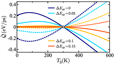
The steady-state heat currents induced by the temperature difference between molecule and metal are shown in Fig. 4 over variation of with held constant. When the temperature of the molecular environment is less than the temperature of the metal, , the heat current into the molecular environment is positive, , and the heat current of the metal is negative, . This is the expected result in which heat moves from the hot environment into the cold environment. At the unithermal point () the heat current vanishes. When , the directionality of the heat current is reversed. The same results for the heat currents can also be obtained using expectation values for the amount of heat transferred by a single electron moving between molecule and metal. See Appendix A for details of this calculation.
IV Electric Current and Thermoelectricity
IV.1 Electric current
To see the implications of the above considerations on the transport properties of a redox molecular junction, we consider a junction in which a molecular species with two electronic states ( and ) is in contact with two metal leads. The left (L) electrode has temperature , the right (R) electrode has temperature , and . The temperature of the molecular species is taken to be , which is an assumption that arises from the postulates that the temperature gradient between the two metals is linear and that the redox molecular site is seated a uniform distance from each electrode. The chemical potentials of the metal electrodes are and .
In this single-molecule two-electrode system, an electron whose charge is localized on the molecule can be transferred to either electrode, and the forward and backward rate constants for these processes are given by evaluating Eqs. (8) and (9) at the corresponding temperatures and chemical potentials. For the left electrode and are evaluated at , and for the right electrode and are evaluated at . The kinetic equations describing the occupation probabilities of states and are
| (22) | ||||
At steady state, the populations of each state can be expressed as
| (23) |
and the steady-state electronic current is Migliore and Nitzan 2011
| (24) |
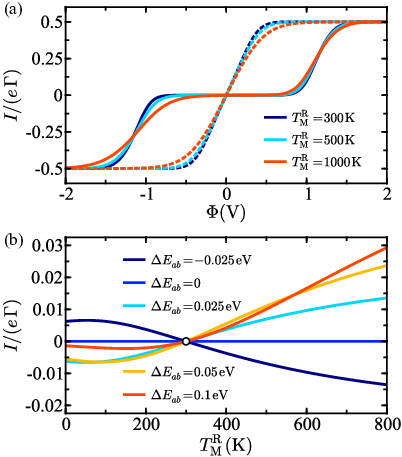
This current is shown in Fig. 5 as function of different system parameters. In Fig. 5(a) it is shown as a function of for various values of with held constant. For , the current is symmetric in the applied voltage , which is an obvious consequence from the symmetry of the structure. However, when and , this symmetry is destroyed. The reason for this is that the contribution to the current induced by the temperature difference depends on the sign of as explained below. For , ), illustrating that asymmetrical effects generated in the junction due to the temperature gradient are dependent on the free energy difference between electronic states in the molecule.
Shown in Fig. 5(b) is the electronic current as function of , keeping constant, at zero bias () for different values of . To understand the observed behavior it should be noted that , given by Eq. (12), corresponds in our model to the single electron energy (the occupation energy) associated with the molecule at nuclear configuration , and its effect on electron transmission depends on the difference . In the present model, where nuclear reorganization is represented by shifted harmonic surfaces, corresponds (for the present choice of ) to the case where , namely to the situation where the single electron “molecular level” at the equilibrium nuclear positions of the occupied state and the unoccupied state are symmetrically seated above and below the Fermi level. This implies that the electron and hole currents are equal in this situation which explains the vanishing of the net current seen in this case. For , the direction of the thermoelectric current (hot to cold or vice versa) depends on the sign of - an extension of the behavior known for electron or hole dominated currents in molecular thermoelectrics.
Nonmonotonic behavior in the electric current can also be observed in Fig. 5(b) with respect to variation of the energy difference between electronic states in the molecular species. In the low-temperature limit (), the magnitude of the current decreases with increasing . In temperature regimes both above and below the unithermal point, the electric current exhibits nonmonotonic trends in which the ordering of with respect to is dependent on the specific value of . In the high-temperature limit (), increasing results in an increased current magnitude.
IV.2 Seebeck coefficient
The standard Seebeck coefficient measures the dependence of the voltage across the junction on the temperature difference between the left and right electrodes, Galperin et al. 2008; Reddy et al. 2007; Tan et al. 2011 calculated about equilibrium under the condition of constant, namely zero, current:
| (25) |
This is most easily evaluated using Eq. (24) and the identity
| (26) |
with all derivatives evaluated at .

The calculated standard “equilibrium” Seebeck coefficient is shown in Fig. 6(a) as a function of . In the limit , it is , which is easily obtained from Eqs. (1) and (2). When , becomes smaller and is a slightly nonlinear function of (note however that linearity is restored for large ). As expected, changes sign with which measures the position of the molecular “single electron level” relative to the metal chemical potential. As , the thermopower in the junction vanishes, implying that without an energy gradient in the electronic states of the molecule, the electric current will vanish, regardless of the imposed temperature difference, which agrees with the results shown in Fig. 5(b). Increasing the reorganization energy , which is a measure of the nuclear-electronic coupling, results in smaller values of , illustrating that stronger coupling leads to lower thermopower in the junction.
The Seebeck coefficient can be calculated outside of the linear limit using the relation Galperin et al. 2008
| (27) |
where is the temperature difference that generates the same current at , as the generates for . Equation (27) is a generalization of the standard definition of the Seebeck coefficient as an attribute of the equilibrium junction to linear response about an arbitrary equilibrium point. The protocol we apply to measure is to change while keeping constant for , and to apply the bias symmetrically across the junction ( and ) for . not Shown in Fig. 6(b) is as a function of , which is the inverse function of , for different reorganization energies and constant . At , the value of is the same as that shown in Fig. 6(a) for the corresponding value of and . As is increased, the Seebeck coefficient increases nonlinearly, which agrees with the behavior observed in Ref. 71 in molecular junctions at the inelastic limit of transport. As is increased further, a turnover is observed for small values of (weak electron-environment interaction), and begins to decrease. This is the same trend that has been observed previously in studies of transport in junctions in the weak electron-phonon coupling limit.Galperin et al. 2008
V Conclusions
A theory has been developed to describe the rate of electron transfer between a molecular species and a metal electrode, with each being at a different local temperature. The rate constant for this process was found to be nonlinear in the temperature of each environment. We find that due the temperature gradient, electron transfer between redox sites carries heat between the metal and the thermal environment of the molecule, and this contribution to the interfacial heat conduction has been characterized. Analogous to previous results observed in bithermal molecule-to-molecule electron transfer reactions, Craven and Nitzan 2016 the electrothermal heat transfer does not vanish when the electric current between molecule and metal reaches a stationary state.
Thermoelectric effects induced by a temperature difference between heterogeneous redox sites have also been investigated. The findings presented here illustrate how electronic and thermal transport are related at the strong-coupling limit, and how electrothermal transport and traditional thermoelectric effects can be induced. Control of transport and amplification in thermal currents has potential applications in the development of novel energy conversion devices and molecular electronics. Operational deficiencies in thermal logic gates and circuits with respect to their electronic analogs occur due to timescale mismatches in phononic transport, which takes place on the time-scale of nuclear motion, and electronic transport. The theory of electrothermal transport presented here can possibly provide rectification of this timescale problem in thermal circuits due to the described heat transfer mechanism occurring on the timescale of electron motion. Further study and validation of this conjecture is required, and in future work we will provide a rigorous comparison of the rates and timescales of phononic and electronic heat transport.
The presented results provide a step toward the ability to completely model electron hopping in molecular junctions in which complex molecular motifs are seated between two electrodes. In future work, we will also present a theory for bithermal electron transfer at the weak-coupling limit in which electron transmission between redox sites occurs on a faster timescale than vibrational relaxation, resulting in energetic distributions that are intrinsically nonequilibrium.
VI Acknowledgments
AN is supported by the Israel Science Foundation, the US-Israel Bi-national Science Foundation and the University of Pennsylvania. AN thanks Prof. Michael Galperin for useful discussions.
Appendix A Heat Current Derivation From Single-Electron Expectation Values
To derive the expectation value for the heat transferred by an electron when it moves between environments, we consider a single electron whose charge is localized on the molecular donor, and the probability for it to enter the metal at energy . This probability depends on multiple independent factors: (a) the probability that the solvent environment is in a configuration in which the electron can be transferred into the metal at energy , (b) the probability that there is a vacancy in the metal at energy , (c) the density of states in the metal at energy , and (d) the probability that the transition between states occurs, which can be calculated using the Landau-Zener expression Nitzan 2006 and thus we denote this probability . In the nonadiabatic limit, the general relationship holds, where is a constant that does not play a role in the calculations that follow, but we include it for completeness.
Because of the occupancy characteristics of each energy level in the metal, the specific electron we consider can make many attempts to enter the metal, at many different energies, before the transfer event occurs. We denote the probability of a successful attempt (meaning ET occurs) for transfer into the metal with energy as where is the Boltzmann weight of energy level that leads to the electron entering the metal at energy , which depends on the temperature of the solvent environment of the molecular species. However, due to the quasicontinuum of energy levels in the electronic manifold of the metal and the occupancy/vacancy probabilities for each of these levels, there are many other possible outcomes for each attempt, and each outcome must be accounted for to derive the amount of heat transferred.
The complexity of this network of events can be simplified by grouping them the into three possible outcomes for each attempt: either the electron enters the metal at energy with probability , the electron enters the metal at an energy that is not , which we denote , or the electron attempts to transfer into the metal at any energy, but there is no vacancy at the respective energy. We term the latter as an unsuccessful attempt and denote the probability for this outcome as . From conservation of probability for each attempt, , we find that . If the first electron transfer attempt is unsuccessful, the electron will eventually make another transfer attempt due to thermal fluctuations. If the second attempt to transfer is also unsuccessful, the electron will make a third attempt, and this process is repeated ad infinitum. If the first attempt is unsuccessful with probability , the probability for success on the second attempt given that the first was unsuccessful is , and the probability for success on a third attempt given that it is preceded by two previous unsuccessful attempts is . Taking the sum of all possible event sequences that lead to the electron entering the metal at energy gives , a geometric series. The sum of this series can be expressed as which gives after substitution for .
This analysis can be performed for each energy level leading to the general expression . Note that this derivation is also valid for the transition in which the electron moves from metal to molecule, provided that the probability of vacancy given by is replaced by the corresponding occupancy probability in each expression.
Using this event analysis to evaluate the probability of all possible transitions from the molecule into the metal, and writing the sums in the expression as integrals, we find that the Fermi-weighted configuration integral for the transition (which corresponds to the denominator in the expression for given above) is
| (28) | ||||
The expectation value of the heat supplied by the environment of the molecular species during the ascent (denoted by ) to the transition state on the surface is
| (29) | ||||
and for the descent (denoted by ) on the surface:
| (30) | ||||
The heat that flows into the metal during the ET process is
| (31) | ||||
Note that if the Fermi factor was not included in , Eqs. (29)-(31) would give the respective expectation value per transition attempt; with its inclusion these equations give the probability per transition event. The heat transferred to the solvent environment over the transition is
| (32) |
The total free energy change by the molecular system and the metal is . Correspondingly, by conservation of energy we expect that the environments must change by . We have verified, numerically, over a variety of parameter values, that the sum of the energy change during each leg of the transition gives
| (33) |
and thus that the expectation value expressions conserve energy.
For the transition, constructing the Fermi-weighted configuration integral yields
| (34) | ||||
The expectation value of the heat supplied by the environment of the molecular species during the ascent to the transition state on the surface is
| (35) | ||||
and for the descent to equilibrium on the surface:
| (36) | ||||
The heat supplied by the metal is
| (37) | ||||
The heat transferred to the solvent environment over the transition is
| (38) |
The sum of the free energy change by the molecular system and the metal is , and thus during this transition the environments must change by . To confirm that our expectation value expressions conserve energy, we take the sum of each process in the transition (using numerically evaluation of the integrals). In all studied cases we have found that
| (39) |
as expected.
References
- Aviram and Ratner (1974) A. Aviram and M. A. Ratner, Chem. Phys. Lett. 29, 277 (1974), eprint doi:10.1016/0009-2614(74)85031-1.
- Carroll and Gorman (2002) R. L. Carroll and C. B. Gorman, Angew. Chem., Ind. Ed. 41, 4378 (2002), eprint doi:10.1002/1521-3773(20021202)41:23¡4378::AID-ANIE4378¿3.0.CO;2-A.
- Nitzan and Ratner (2003) A. Nitzan and M. A. Ratner, Science 300, 1384 (2003), eprint doi:10.1126/science.1081572.
- Coropceanu et al. (2007) V. Coropceanu, J. Cornil, D. A. da Silva Filho, Y. Olivier, R. Silbey, and J.-L. Brédas, Chem. Rev. 107, 926 (2007).
- Galperin et al. (2007a) M. Galperin, M. A. Ratner, and A. Nitzan, J. Phys.: Condens. Matter 19, 103201 (2007a).
- Dubi and Di Ventra (2011) Y. Dubi and M. Di Ventra, Rev. Mod. Phys. 83, 131 (2011), eprint doi:10.1103/RevModPhys.83.131.
- Galperin et al. (2007b) M. Galperin, A. Nitzan, and M. A. Ratner, Phys. Rev. B 75, 155312 (2007b), eprint doi:10.1103/PhysRevB.75.155312.
- Galperin et al. (2009) M. Galperin, K. Saito, A. V. Balatsky, and A. Nitzan, Phys. Rev. B 80, 115427 (2009), eprint doi:10.1103/PhysRevB.80.115427.
- Galperin and Nitzan (2011a) M. Galperin and A. Nitzan, J. Phys. Chem. Lett. 2, 2110 (2011a), eprint doi:10.1021/jz2008853.
- Galperin and Nitzan (2011b) M. Galperin and A. Nitzan, Phys. Rev. B 84, 195325 (2011b), eprint doi:10.1103/PhysRevB.84.195325.
- Horsfield et al. (2006) A. P. Horsfield, D. R. Bowler, H. Ness, C. G. Sánchez, T. N. Todorov, and A. J. Fisher, Rep. Prog. Phys. 69, 1195 (2006).
- D’Agosta and Ventra (2008) R. D’Agosta and M. D. Ventra, J. Phys.: Condens. Matter 20, 374102 (2008).
- Asai (2011) Y. Asai, Phys. Rev. B 84, 085436 (2011), eprint doi:10.1103/PhysRevB.84.085436.
- Asai (2015) Y. Asai, Phys. Rev. B 91, 161402 (2015), eprint doi:10.1103/PhysRevB.91.161402.
- Lake and Datta (1992) R. Lake and S. Datta, Phys. Rev. B 46, 4757 (1992), eprint doi:10.1103/PhysRevB.46.4757.
- Härtle and Thoss (2011) R. Härtle and M. Thoss, Phys. Rev. B 83, 115414 (2011), eprint doi:10.1103/PhysRevB.83.115414.
- Lu et al. (2015) J.-T. Lu, H. Zhou, J.-W. Jiang, and J.-S. Wang, AIP Adv. 5, 053204 (2015), eprint doi:10.1063/1.4917017.
- Cahill et al. (2002) D. G. Cahill, K. Goodson, and A. Majumdar, J. Heat Transfer 124, 223 (2002).
- Cahill et al. (2003) D. G. Cahill, W. K. Ford, K. E. Goodson, G. D. Mahan, A. Majumdar, H. J. Maris, R. Merlin, and S. R. Phillpot, J. Appl. Phys. 93, 793 (2003), eprint doi:10.1063/1.1524305.
- Leitner (2008) D. M. Leitner, Annu. Rev. Phys. Chem. 59, 233 (2008), eprint doi:10.1146/annurev.physchem.59.032607.093606.
- Leitner (2013) D. M. Leitner, J. Phys. Chem. B 117, 12820 (2013), eprint doi:10.1021/jp402012z.
- Leitner (2015) D. M. Leitner, Adv. Phys. 64, 445 (2015), eprint doi:10.1080/00018732.2015.1109817.
- Li et al. (2012) N. Li, J. Ren, L. Wang, G. Zhang, P. Hänggi, and B. Li, Rev. Mod. Phys. 84, 1045 (2012), eprint doi:10.1103/RevModPhys.84.1045.
- Dhar (2008) A. Dhar, Adv. Phys. 57, 457 (2008), eprint doi:10.1080/00018730802538522.
- Luo and Chen (2013) T. Luo and G. Chen, Phys. Chem. Chem. Phys. 15, 3389 (2013), eprint doi:10.1039/C2CP43771F.
- Rubtsova et al. (2015a) N. I. Rubtsova, L. N. Qasim, A. A. Kurnosov, A. L. Burin, and I. V. Rubtsov, Acc. Chem. Res. 48, 2547 (2015a), eprint doi:10.1021/acs.accounts.5b00299.
- Rubtsova et al. (2015b) N. I. Rubtsova, C. M. Nyby, H. Zhang, B. Zhang, X. Zhou, J. Jayawickramarajah, A. L. Burin, and I. V. Rubtsov, J. Chem. Phys. 142, 212412 (2015b), eprint doi:10.1063/1.4916326.
- Chen et al. (2003) Y.-C. Chen, M. Zwolak, and M. Di Ventra, Nano Lett. 3, 1691 (2003), eprint doi:10.1021/nl0348544.
- Pecchia et al. (2007) A. Pecchia, G. Romano, and A. Di Carlo, Phys. Rev. B 75, 035401 (2007), eprint doi:10.1103/PhysRevB.75.035401.
- Yang et al. (2012) N. Yang, X. Xu, G. Zhang, and B. Li, AIP Adv. 2, 041410 (2012), eprint doi:10.1063/1.4773462.
- Zimbovskaya (2016) N. A. Zimbovskaya, J. Phys.: Condens. Matter 28, 183002 (2016), eprint http://stacks.iop.org/0953-8984/28/i=18/a=183002.
- Li et al. (2004) B. Li, L. Wang, and G. Casati, Phys. Rev. Lett. 93, 184301 (2004), eprint doi:10.1103/PhysRevLett.93.184301.
- Segal and Nitzan (2005) D. Segal and A. Nitzan, J. Chem. Phys. 122, 194704 (2005), eprint doi:10.1063/1.1900063.
- Chang et al. (2006) C. W. Chang, D. Okawa, A. Majumdar, and A. Zettl, Science 314, 1121 (2006), eprint doi:10.1126/science.1132898.
- Segal (2008) D. Segal, Phys. Rev. Lett. 100, 105901 (2008), eprint doi:10.1103/PhysRevLett.100.105901.
- Wu and Segal (2009) L.-A. Wu and D. Segal, Phys. Rev. Lett. 102, 095503 (2009), eprint doi:10.1103/PhysRevLett.102.095503.
- Zhong et al. (2009) W.-R. Zhong, P. Yang, B.-Q. Ai, Z.-G. Shao, and B. Hu, Phys. Rev. E 79, 050103 (2009), eprint doi:10.1103/PhysRevE.79.050103.
- Ren and Zhu (2013) J. Ren and J.-X. Zhu, Phys. Rev. B 87, 241412 (2013), eprint doi:10.1103/PhysRevB.87.241412.
- Ming et al. (2016) Y. Ming, H.-M. Li, and Z.-J. Ding, Phys. Rev. E 93, 032127 (2016), eprint doi:10.1103/PhysRevE.93.032127.
- Arrachea et al. (2014) L. Arrachea, N. Bode, and F. von Oppen, Phys. Rev. B 90, 125450 (2014), eprint doi:10.1103/PhysRevB.90.125450.
- Li et al. (2015) Q. Li, I. Duchemin, S. Xiong, G. C. Solomon, and D. Donadio, J. Phys. Chem. C 119, 24636 (2015), eprint doi:10.1021/acs.jpcc.5b07429.
- Delor et al. (2014) M. Delor, P. A. Scattergood, I. V. Sazanovich, A. W. Parker, G. M. Greetham, A. J. H. M. Meijer, M. Towrie, and J. A. Weinstein, Science 346, 1492 (2014), eprint doi:10.1126/science.1259995.
- Vlc̆ek Jr. et al. (2015) A. Vlc̆ek Jr., H. Kvapilová, M. Towrie, and S. Zális̆, Acc. Chem. Res. 48, 868 (2015), eprint doi:10.1021/ar5004048.
- Bakulin et al. (2015) A. A. Bakulin, R. Lovrincic, X. Yu, O. Selig, H. J. Bakker, Y. L. Rezus, P. K. Nayak, A. Fonari, V. Coropceanu, J.-L. Brédas, et al., Nat. Commun. 6, 7880 (2015), eprint doi:10.1038/ncomms8880.
- Ren et al. (2012) J. Ren, J.-X. Zhu, J. E. Gubernatis, C. Wang, and B. Li, Phys. Rev. B 85, 155443 (2012), eprint doi:10.1103/PhysRevB.85.155443.
- Walczak (2007) K. Walczak, Physica B 392, 173 (2007), ISSN 0921-4526, eprint doi:10.1016/j.physb.2006.11.013.
- Koch et al. (2014) T. Koch, J. Loos, and H. Fehske, Phys. Rev. B 89, 155133 (2014), eprint doi:10.1103/PhysRevB.89.155133.
- Perroni et al. (2014) C. A. Perroni, D. Ninno, and V. Cataudella, Phys. Rev. B 90, 125421 (2014), eprint doi:10.1103/PhysRevB.90.125421.
- Zimbovskaya (2014) N. A. Zimbovskaya, J. Phys.: Condens. Matter 26, 275303 (2014).
- Migliore and Nitzan (2013) A. Migliore and A. Nitzan, J. Am. Chem. Soc. 135, 9420 (2013), eprint doi:10.1021/ja401336u.
- Marcus (1956) R. A. Marcus, J. Chem. Phys. 24, 966 (1956), eprint doi:10.1063/1.1742723.
- Marcus (1964) R. A. Marcus, Annu. Rev. Phys. Chem. 15, 155 (1964), eprint doi:10.1146/annurev.pc.15.100164.001103.
- Marcus and Sutin (1985) R. A. Marcus and N. Sutin, Biochim. Biophys. Acta 811, 265 (1985), eprint doi:10.1016/0304-4173(85)90014-X.
- Marcus (1993) R. A. Marcus, Rev. Mod. Phys. 65, 599 (1993), eprint doi:10.1103/RevModPhys.65.599.
- Peters (2015) B. Peters, J. Phys. Chem. B 119, 6349 (2015), eprint doi:10.1021/acs.jpcb.5b02547.
- Craven and Nitzan (2016) G. T. Craven and A. Nitzan, Proc. Natl. Acad. Sci. 113, 9421 (2016), eprint doi:10.1073/pnas.1609141113.
- Craven and Nitzan (2017) G. T. Craven and A. Nitzan, Phys. Rev. Lett. 118, 207201 (2017), eprint doi:10.1103/PhysRevLett.118.207201.
- Nitzan (2006) A. Nitzan, Chemical Dynamics in Condensed Phases: Relaxation, Transfer, and Reactions in Condensed Molecular Systems (Oxford University Press, 2006).
- Marcus (1965) R. A. Marcus, J. Chem. Phys. 43, 679 (1965), eprint doi:10.1063/1.1696792.
- Stähler et al. (2007) J. Stähler, M. Meyer, X. Y. Zhu, U. Bovensiepen, and M. Wolf, New J. Phys. 9, 394 (2007), eprint doi:10.1088/1367-2630/9/10/394.
- Zeng et al. (2014) Y. Zeng, R. B. Smith, P. Bai, and M. Z. Bazant, J. Electroanal. Chem. 735, 77 (2014), ISSN 1572-6657, eprint doi:10.1016/j.jelechem.2014.09.038.
- Zanetti-Polzi and Corni (2016) L. Zanetti-Polzi and S. Corni, Phys. Chem. Chem. Phys. 18, 10538 (2016), eprint doi:10.1039/C6CP00044D.
- Hupp and Weaver (1984) J. T. Hupp and M. J. Weaver, J. Phys. Chem. 88, 6128 (1984), eprint doi:10.1021/j150669a015.
- Laborda et al. (2012) E. Laborda, M. C. Henstridge, and R. G. Compton, J. Electroanal. Chem. 667, 48 (2012), ISSN 1572-6657, eprint doi:10.1016/j.jelechem.2011.12.011.
- Laborda et al. (2013) E. Laborda, M. C. Henstridge, C. Batchelor-McAuley, and R. G. Compton, Chem. Soc. Rev. 42, 4894 (2013), eprint doi:10.1039/C3CS35487C.
- Hush (1968) N. Hush, Electrochim. Acta 13, 1005 (1968), eprint doi:10.1016/0013-4686(68)80032-5.
- Chidsey (1991) C. E. D. Chidsey, Science 251, 919 (1991), eprint doi:10.1126/science.251.4996.919.
- Migliore and Nitzan (2011) A. Migliore and A. Nitzan, ACS Nano 5, 6669 (2011), eprint doi:10.1021/nn202206e.
- Migliore et al. (2012) A. Migliore, P. Schiff, and A. Nitzan, Phys. Chem. Chem. Phys. 14, 13746 (2012), eprint doi:10.1039/C2CP41442B.
- Reddy et al. (2007) P. Reddy, S.-Y. Jang, R. A. Segalman, and A. Majumdar, Science 315, 1568 (2007), eprint doi:10.1126/science.1137149.
- Galperin et al. (2008) M. Galperin, A. Nitzan, and M. A. Ratner, Mol. Phys. 106, 397 (2008), eprint doi:10.1080/00268970701837784.
- Ke et al. (2009) S.-H. Ke, W. Yang, S. Curtarolo, and H. U. Baranger, Nano Lett. 9, 1011 (2009), eprint doi:10.1021/nl8031229.
- Liu and Chen (2009) Y.-S. Liu and Y.-C. Chen, Phys. Rev. B 79, 193101 (2009), eprint doi:10.1103/PhysRevB.79.193101.
- Sadat et al. (2010) S. Sadat, A. Tan, Y. J. Chua, and P. Reddy, Nano Lett. 10, 2613 (2010), eprint doi:10.1021/nl101354e.
- Tan et al. (2011) A. Tan, J. Balachandran, S. Sadat, V. Gavini, B. D. Dunietz, S.-Y. Jang, and P. Reddy, J. Am. Chem. Soc. 133, 8838 (2011), eprint doi:10.1021/ja202178k.
- Kim et al. (2014) Y. Kim, W. Jeong, K. Kim, W. Lee, and P. Reddy, Nature Nanotech. 9, 881 (2014), eprint doi:10.1038/nnano.2014.209.
- Lee et al. (2014) E.-S. Lee, S. Cho, H.-K. Lyeo, and Y.-H. Kim, Phys. Rev. Lett. 112, 136601 (2014), eprint doi:10.1103/PhysRevLett.112.136601.
- Koch et al. (2004) J. Koch, F. von Oppen, Y. Oreg, and E. Sela, Phys. Rev. B 70, 195107 (2004), eprint doi:10.1103/PhysRevB.70.195107.
- Simine et al. (2015) L. Simine, W. J. Chen, and D. Segal, J. Phys. Chem. C 119, 12097 (2015), eprint doi:10.1021/jp512648f.
- (80) It is important to note that these results depend on the protocol used to define and . We will expand on this issue in a future paper.