Electrothermal Transistor Effect and Cyclic Electronic Currents
in Multithermal Charge Transfer Networks
Abstract
A theory is developed to describe the coupled transport of energy and charge in networks of electron donor-acceptor sites which are seated in a thermally heterogeneous environment, where the transfer kinetics are dominated by Marcus-type hopping rates. It is found that the coupling of heat and charge transfer in such systems gives rise to exotic transport phenomena which are absent in thermally homogeneous systems and cannot be described by standard thermoelectric relations. Specifically, the directionality and extent of thermal transistor amplification and cyclical electronic currents in a given network can be controlled by tuning the underlying temperature gradient in the system. The application of these findings toward optimal control of multithermal currents is illustrated on a paradigmatic nanostructure.
- Cite as
-
G. T. Craven and A. Nitzan, Phys. Rev. Lett. 118, 207201 (2017)
- DOI
The coupling between electron transfer (ET) and transport and the underlying thermal environment is a long studied subject Galperin et al. 2007. Its manifestations in recent studies of transport in molecular junctions mostly focus on the weak electron-phonon coupling regime. Similarly, thermoelectric phenomena in such junctions Dubi and Di Ventra 2011, where molecules connect between electrodes of different temperatures, are usually treated (with a few exceptions, e.g., Refs. Walczak 2007; Galperin et al. 2008; Wang et al. 2011; Ren et al. 2012; Tagani and Soleimani 2012; Tagani and Soleimani 2013; Perroni et al. 2014; Perroni et al. 2015; Koch et al. 2014; Zimbovskaya 2016) with electron-vibration interaction disregarded. This stands in contrast to electron transfer reactions in condensed molecular systems that are usually dominated by hopping between thermally equilibrated polaron-like states as described by Marcus theory Marcus 1956; Marcus 1964; Nitzan 2006; Peters 2015 (analogous kinetics in junction transport is known, mostly in so called redox molecular junctions Zhang et al. 2008; Migliore and Nitzan 2013). We have recently considered the latter type of electronic transport in thermally heterogeneous systems, where an electron hops between two sites of different local temperatures Craven and Nitzan 2016. This study was motivated by recent advances in measurement and control of temperature differences on length scales comparable to those involved in molecular electron transfer processes Chang et al. 2006; Sadat et al. 2010; Malen et al. 2010; Tan et al. 2011; Lee et al. 2013; Kim et al. 2014. The corresponding ET rate was obtained as a modified multidimensional Marcus expression that depends on the local temperatures of the two sites. Furthermore, electron hopping was shown to to be accompanied by heat transfer between the sites whose magnitude depends on the temperature difference and on the reorganization (polaron formation) energies at the two sites.
Thermal inhomogeneity can develop spontaneously in driven nonequilibrium systems Popov and Hernandez 2007; Jarzynski 2015; Craven and Hernandez 2015; Li et al. 2015; Einax and Nitzan 2016 or can be externally controlled as in a thermoelectric device. Considering such models, several recent theoretical studies have discovered interesting thermal transistor effects, whereupon the flux between two sites can be controlled by the temperature on a third site Li et al. 2006; Ben-Abdallah and Biehs 2014; Joulain et al. 2016.
In this Letter, we develop a theory to describe ET in complex networks of donor-acceptor sites, where each site is associated with normal modes that are in contact with an independent heat bath at the local site temperature. This is an idealization of the standard phenomenology of molecular electron transfer where the electronic processes is most strongly coupled to vibrations that are localized on the donor and acceptor sites. In the limit of strong electron-phonon coupling, electron transport is dominated by hopping-type events and Marcus theory gives the conceptual basis, and sometimes quantitative understanding, of ET reactions Marcus 1956; Marcus 1964; Nitzan 2006; Peters 2015. The multithermal nature of the examined systems arises because the donor and acceptor sites can be at different temperatures. Purely vibrational heat transfer between sites is disregarded for simplicity, so in what follows we focus on electron transfer and the associated heat transfer Craven and Nitzan 2016; Matyushov 2016. The development of complex network theory Schnakenberg 1976 has significantly increased our understanding of the flow of charge, energy, and information in diverse types of systems Strogatz 2001; Albert and Barabási 2002; Estrada and Hatano 2007; Gao et al. 2011; Solomon et al. 2010; Rai et al. 2011; Rai et al. 2012; Savoie et al. 2014; Einax and Nitzan 2014; Hansen and Solomon 2016 and the present study makes it possible to consider electron and heat transport within such a framework and to study the consequence of their interdependence.
The donor-acceptor networks we consider consist of sites, where each site , which has local temperature , is associated with harmonic modes that are equilibrated with the thermal environment about that site. Specifically, we consider transitions between electronic states for which an excess electron is localized on different sites of this network. In the Marcus picture Marcus 1956 of ET, the localized occupation of electron density associated with electronic state of the network is described by the energy surface
| (1) |
where is an electronic energy origin of state , is the coordinate of the th vibrational mode, and is a shift in the equilibrium position of the th mode. Both and are measured relative to some reference state for which and vanish (properties of this state do not affect the final results). The total number of modes in the system is denoted by and the group of modes associated with the th site is . In a likely special case unless mode is localized about the site on which the electron is placed in state (that is, unless and is the electronic state that corresponds to the electron occupying site ). However, the form (1) can represent more general situations where the modes localized about site respond to the electronic occupation on a different site. A transition between states and is associated with a reorganization energy (assumed temperature independent) in the th mode, , and a total reorganization energy, , which are given by:
| (2) |
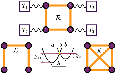
The shifts , and hence the reorganization energies, of a system depend on the intersite distances and therefore the topology of the underlying connectivity network. Shown in Fig. 1 are representative topologies for three typical connectivities: ring , linear , and complete . Associated with each network is an adjacency matrix where if sites and are connected (and thus the electron can tunnel between sites) and is zero otherwise Schnakenberg 1976. The topology of determines which modes are responsive to electron localization on a particular site. We next show that temperature differences between sites give rise to emergent and sometimes exotic thermal and electronic transport properties.
The electron transfer rate between any two sites in the network and the heat transfer rate between the thermal baths involved in this transition can be derived by adopting the formalism put forth in Ref. 19 for bithermal electron hopping between two sites. “Involved bath” implies that the harmonic modes that are thermalized by this bath are sensitive to the electronic population of at least one of the sites. Under standard transition state theory assumptions the rate of the transition can be expressed as
| (3) |
where is the tunneling probability between states, is the probability density about a transition surface (TS) separating the states, both evaluated on the surface, and is the velocity in the direction normal to the TS Hammes-Schiffer and Tully 1995; Jóhannesson and Jónsson 2001. The normal velocity where is a unit vector normal to the TS at position on this hypersurface. The factor is a (multi)thermal average that depends on the temperature of each bath involved in the transition. The TS is determined by the requirement that a transition can only take place at nuclear configurations where electronic energy is conserved. For the -dimensional paraboloid energy surface defined by (1), the TS separating states is an -dimensional transition state hypersurface which is the locus of mode configurations where , defined by .
In the adiabatic limit of Marcus rate theory and the pre-exponential factor is proportional to not a. In the nonadiabatic limit not b, can be approximated by the corresponding limit of the Landau-Zener expression Thompson 1998; Nitzan 2006; Lykhin et al. 2016 which is evaluated in the direction normal to the TS Marks and Thompson 1992. In this limit, , and the expectation value does not depend on the normal velocity not c. For the transition, the multithermal probability to be on the TS is:
| (4) | ||||
where with being the Boltzmann constant. The -function in (4) constrains the integration over the vibrational subspace in which and the gradient magnitude gives a precise definition to this constraint Hartmann et al. 2011. Evaluating the integrals in Eq. (4) we obtain
| (5) | ||||
which expresses the probability density on the reaction path in terms of the temperature of each bath, and the reorganization energy and reaction free energy of the respective transition. In the uniform temperature limit, combining Eqs. (3) and (5) recovers the Marcus rate Marcus 1956; Marcus 1964; Nitzan 2006; Peters 2015.
With the multidimensional-multithermal transition rate now derived, the kinetic equations for the occupation probability of each state can be constructed. For a reaction network (see Fig. 1) with adjacency matrix these equations take the form
| (6) |
for each state . At steady-state , which implies that the net electronic flux between sites vanishes.
Next consider the heat transfer associated with a given electron transfer step Craven and Nitzan 2016; Craven and Nitzan 2017. In Marcus theory, the nuclear motion leading to the transition proceeds through a point on the TS, and the corresponding heat transferred into a specific bath during the transition is where the first term is the heat obtained from the bath during the ascent to on the surface and the second term is the heat released to the bath during the descent to equilibrium on the surface (see Fig. 1). Using the energy surfaces of Eq. (1), the contribution of mode to the net heat exchange with the bath associated with it during the transition is given by
| (7) |
This quantity should be averaged over the probability to reach the particular configuration on the TS when coming from the side:
| (8) |
where is the probability density on the TS when the system is in state not a:
| (9) | ||||
Evaluating the expectation integral gives
| (10) |
where if . The total heat transferred to the thermal environment of site during the transition is the sum of contributions over all modes associated with that site:
| (11) | ||||
Here, the term proportional to expresses the heat released to/taken from the baths from the free energy difference between these electronic states, while the term proportional to is the actual heat transfer between baths and associated with the transition.
The heat current into the thermal environment of site is
| (12) |
Note that while , the expectation value of and the heat current can be either positive or negative implying that the corresponding bath absorbs or releases energy, respectively. In unithermal systems at steady-state the heat currents vanish (), while in contrast, for multithermal systems, and thus . Note that even as the occupation probabilities approach electronic quasi-equilibrium where the net electronic currents are zero, the net flow of heat does not vanish. This phenomenon is not a standard thermoelectric effect and reveals a novel pathway for energy transport in multithermal charge transfer networks.

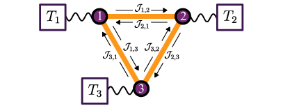
Another interesting behavior that is observed in multithermal networks with closed loops is the persistence of steady-state net electronic bond currents, , i.e., the breaking of detailed balance, and the formation of cyclical current loops that obviously vanish in full equilibrium where detailed balance is maintained. An example is seen in the three-site ring () shown in Fig. 2. We emphasize this simple system because of its experimental realizability and its general applications in molecular electronics and devices Li et al. 2012; Joulain et al. 2016; Allahverdyan et al. 2016, but note that other more complex networks can also be analyzed using the developed theory not e. In a multithermal network, the direction and magnitude of the cyclic flux can be altered by tuning the temperature . This is illustrated in Fig. 3(a) where the donor and acceptor sites 1,2 are at the same temperature while variation of the temperature on another site, , determines the direction and magnitude of the cyclical current. We find that this thermally-induced current persists, except in the case that the electronic occupation energy is the same for all sites involved in the cycle. Note that at the unithermal point in Figs. 3(a)-(b), for every connection, so . This is simply a statement that with no temperature gradient there is no heat current or cyclic electron flux. Similar trends are also observed in Figs. 3(c)-(d) for networks where the local temperature of each site is different. By comparing the temperatures at which in Fig. 3(c) with the heat currents at the same temperature in Fig. 3(d) it can be seen that even when the electron flux vanishes there is still a net heat flow between baths. At full equilibrium, which is achieved in the uniform temperature limit, all electronic and heat fluxes vanish.

The theory of coupled electron and heat transfer developed in this Letter can also be applied to elucidate the electronic contribution to transport phenomena in thermal transistors Li et al. 2006; Ben-Abdallah and Biehs 2014; Joulain et al. 2016, which are recently studied model devices that can be used to control and amplify heat flow. Following Ref. 31, we quantify the magnitude of amplification in thermal transistors by the factor , which measures the effect of pumping heat into site 3 on the heat current between sites 1 and 2. If a transistor effect is present. In the three-site system, variation of the heat current by alteration of can give rise to significant amplifications, as shown in Fig. 4(a). The reason for the electrothermal transistor effect is shown in Fig. 4(b), where at while for as this limit is approached. This aligns with the region of amplification shown in Fig. 4(a).
We have shown that in nanoscale systems where localized modes are in contact with environments at different temperatures, complex nonlinearities in the thermal gradient can induce currents which are characterized by multiple temperatures. A theory has been developed to unify the description of heat and charge transfer in these systems with multithermal temperature gradients between donor-acceptor states. This work provides a bridge connecting theories of electron transfer, heat transport, and thermoelectricity in systems where electron transport is dominated by intersite hopping, and will be useful in the design of electronic and thermoelectric devices that operate in this limit.
In regimes where the magnitude of heat conduction due to electron transport dominates over the magnitude of conduction from phonons, the developed theory will be directly applicable. Otherwise, a complete picture of the conduction process will require a theory that considers both electrothermal and phononic heat transport, and their coupling. Examination of thermopower, efficiency, and their relation to electrothermal transport in molecular junctions (and other complex donor/acceptor networks with molecule-metal and molecule-semiconductor interfaces) in the phonon-assisted hopping limit of electronic transport is a potential application of the present theory Jia et al. 2016; Gagorik et al. 2017; Craven and Nitzan 2017. Generalizations that go beyond the semiclassical Marcus treatment are obviously needed and will be taken on in future work.
AN is supported by the Israel Science Foundation, the US-Israel Binational Science Foundation and the University of Pennsylvania.
References
- Galperin et al. (2007) M. Galperin, M. A. Ratner, and A. Nitzan, J. Phys.: Condens. Matter 19, 103201 (2007).
- Dubi and Di Ventra (2011) Y. Dubi and M. Di Ventra, Rev. Mod. Phys. 83, 131 (2011), eprint doi:10.1103/RevModPhys.83.131.
- Walczak (2007) K. Walczak, Physica B 392, 173 (2007), ISSN 0921-4526, eprint doi:10.1016/j.physb.2006.11.013.
- Galperin et al. (2008) M. Galperin, A. Nitzan, and M. A. Ratner, Mol. Phys. 106, 397 (2008), eprint doi:10.1080/00268970701837784.
- Wang et al. (2011) Y. Wang, J. Zhou, and R. Yang, J. Phys. Chem. C 115, 24418 (2011), eprint doi:10.1021/jp208490q.
- Ren et al. (2012) J. Ren, J.-X. Zhu, J. E. Gubernatis, C. Wang, and B. Li, Phys. Rev. B 85, 155443 (2012), eprint doi:10.1103/PhysRevB.85.155443.
- Tagani and Soleimani (2012) M. B. Tagani and H. R. Soleimani, J. Appl. Phys. 112, 103719 (2012), eprint doi:10.1063/1.4767376.
- Tagani and Soleimani (2013) M. B. Tagani and H. R. Soleimani, Physica B 413, 86 (2013), eprint doi:10.1016/j.physb.2013.01.007.
- Perroni et al. (2014) C. A. Perroni, D. Ninno, and V. Cataudella, Phys. Rev. B 90, 125421 (2014), eprint doi:10.1103/PhysRevB.90.125421.
- Perroni et al. (2015) C. A. Perroni, D. Ninno, and V. Cataudella, New J. Phys. 17, 083050 (2015), eprint http://iopscience.iop.org/article/10.1088/1367-2630/17/8/083050.
- Koch et al. (2014) T. Koch, J. Loos, and H. Fehske, Phys. Rev. B 89, 155133 (2014), eprint doi:10.1103/PhysRevB.89.155133.
- Zimbovskaya (2016) N. A. Zimbovskaya, J. Phys.: Condens. Matter 28, 183002 (2016), eprint http://stacks.iop.org/0953-8984/28/i=18/a=183002.
- Marcus (1956) R. A. Marcus, J. Chem. Phys. 24, 966 (1956), eprint doi:10.1063/1.1742723.
- Marcus (1964) R. A. Marcus, Annu. Rev. Phys. Chem. 15, 155 (1964), eprint doi:10.1146/annurev.pc.15.100164.001103.
- Nitzan (2006) A. Nitzan, Chemical Dynamics in Condensed Phases: Relaxation, Transfer, and Reactions in Condensed Molecular Systems (Oxford University Press, 2006).
- Peters (2015) B. Peters, J. Phys. Chem. B 119, 6349 (2015), eprint doi:10.1021/acs.jpcb.5b02547.
- Zhang et al. (2008) J. Zhang, A. M. Kuznetsov, I. G. Medvedev, Q. Chi, T. Albrecht, P. S. Jensen, and J. Ulstrup, Chem. Rev. 108, 2737 (2008), eprint doi:10.1021/cr068073+.
- Migliore and Nitzan (2013) A. Migliore and A. Nitzan, J. Am. Chem. Soc. 135, 9420 (2013), eprint doi:10.1021/ja401336u.
- Craven and Nitzan (2016) G. T. Craven and A. Nitzan, Proc. Natl. Acad. Sci. 113, 9421 (2016), eprint doi:10.1073/pnas.1609141113.
- Chang et al. (2006) C. W. Chang, D. Okawa, A. Majumdar, and A. Zettl, Science 314, 1121 (2006), eprint doi:10.1126/science.1132898.
- Sadat et al. (2010) S. Sadat, A. Tan, Y. J. Chua, and P. Reddy, Nano Lett. 10, 2613 (2010), eprint doi:10.1021/nl101354e.
- Malen et al. (2010) J. A. Malen, S. K. Yee, A. Majumdar, and R. A. Segalman, Chem. Phys. Lett. 491, 109 (2010), eprint doi:10.1016/j.cplett.2010.03.028.
- Tan et al. (2011) A. Tan, J. Balachandran, S. Sadat, V. Gavini, B. D. Dunietz, S.-Y. Jang, and P. Reddy, J. Am. Chem. Soc. 133, 8838 (2011), eprint doi:10.1021/ja202178k.
- Lee et al. (2013) W. Lee, K. Kim, W. Jeong, L. A. Zotti, F. Pauly, J. C. Cuevas, and P. Reddy, Nature 498, 209 (2013), eprint doi:10.1038/nature12183.
- Kim et al. (2014) Y. Kim, W. Jeong, K. Kim, W. Lee, and P. Reddy, Nature Nanotech. 9, 881 (2014), eprint doi:10.1038/nnano.2014.209.
- Popov and Hernandez (2007) A. V. Popov and R. Hernandez, J. Chem. Phys. 126, 244506 (2007), eprint doi:10.1063/1.2743032.
- Jarzynski (2015) C. Jarzynski, Nature Phys. 11, 105 (2015), eprint doi:10.1038/nphys3229.
- Craven and Hernandez (2015) G. T. Craven and R. Hernandez, Phys. Rev. Lett. 115, 148301 (2015), eprint doi:10.1103/PhysRevLett.115.148301.
- Li et al. (2015) Q. Li, I. Duchemin, S. Xiong, G. C. Solomon, and D. Donadio, J. Phys. Chem. C 119, 24636 (2015), eprint doi:10.1021/acs.jpcc.5b07429.
- Einax and Nitzan (2016) M. Einax and A. Nitzan, J. Chem. Phys. 145, 014108 (2016), eprint doi:10.1063/1.4955160.
- Li et al. (2006) B. Li, L. Wang, and G. Casati, Appl. Phys. Lett. 88, 143501 (2006), eprint doi:10.1063/1.2191730.
- Ben-Abdallah and Biehs (2014) P. Ben-Abdallah and S.-A. Biehs, Phys. Rev. Lett. 112, 044301 (2014), eprint doi:10.1103/PhysRevLett.112.044301.
- Joulain et al. (2016) K. Joulain, J. Drevillon, Y. Ezzahri, and J. Ordonez-Miranda, Phys. Rev. Lett. 116, 200601 (2016), eprint doi:10.1103/PhysRevLett.116.200601.
- Matyushov (2016) D. V. Matyushov, Proc. Natl. Acad. Sci. 113, 9401 (2016), eprint doi:10.1073/pnas.1610542113.
- Schnakenberg (1976) J. Schnakenberg, Rev. Mod. Phys. 48, 571 (1976), eprint doi:10.1103/RevModPhys.48.571.
- Strogatz (2001) S. H. Strogatz, Nature 410, 268 (2001), eprint doi:10.1038/35065725.
- Albert and Barabási (2002) R. Albert and A.-L. Barabási, Rev. Mod. Phys. 74, 47 (2002), eprint doi:10.1103/RevModPhys.74.47.
- Estrada and Hatano (2007) E. Estrada and N. Hatano, Chem. Phys. Lett. 439, 247 (2007), eprint doi:10.1016/j.cplett.2007.03.098.
- Gao et al. (2011) J. Gao, S. V. Buldyrev, S. Havlin, and H. E. Stanley, Phys. Rev. Lett. 107, 195701 (2011), eprint doi:10.1103/PhysRevLett.107.195701.
- Solomon et al. (2010) G. C. Solomon, C. Herrmann, T. Hansen, V. Mujica, and M. A. Ratner, Nature Chem. 2, 223 (2010), eprint doi:10/1038/nchem.546.
- Rai et al. (2011) D. Rai, O. Hod, and A. Nitzan, J. Phys. Chem. Lett. 2, 2118 (2011), eprint doi:10.1021/jz200862r.
- Rai et al. (2012) D. Rai, O. Hod, and A. Nitzan, Phys. Rev. B 85, 155440 (2012), eprint doi:10.1103/PhysRevB.85.155440.
- Savoie et al. (2014) B. M. Savoie, K. L. Kohlstedt, N. E. Jackson, L. X. Chen, M. Olvera de la Cruz, G. C. Schatz, T. J. Marks, and M. A. Ratner, Proc. Natl. Acad. Sci. 111, 10055 (2014), eprint doi:10.1073/pnas.1409514111.
- Einax and Nitzan (2014) M. Einax and A. Nitzan, J. Phys. Chem. C 118, 27226 (2014), eprint doi:10.1021/jp5084373.
- Hansen and Solomon (2016) T. Hansen and G. C. Solomon, J. Phys. Chem. C 120, 6295 (2016), eprint doi:10.1021/acs.jpcc.5b11211.
- Hammes-Schiffer and Tully (1995) S. Hammes-Schiffer and J. C. Tully, J. Chem. Phys. 103, 8528 (1995), eprint doi:10.1063/1.470162.
- Jóhannesson and Jónsson (2001) G. H. Jóhannesson and H. Jónsson, J. Chem. Phys. 115, 9644 (2001), eprint doi:10.1063/1.1415499.
- not (a) See the Supplemental Material for detailed derivations of each component in the rate and heat transfer expressions.
- not (b) For experimental setups in which sites of appreciably different temperatures are relatively far from each other, implying relatively weak electronic coupling, the nonadiabatic limit will be the most pertinent.
- Thompson (1998) D. L. Thompson, Modern Methods for Multidimensional Dynamics Computations in Chemistry (World Scientific, 1998).
- Lykhin et al. (2016) A. O. Lykhin, D. S. Kaliakin, G. E. dePolo, A. A. Kuzubov, and S. A. Varganov, Int. J. Quantum Chem. 116, 750 (2016), eprint doi:10.1002/qua.25124.
- Marks and Thompson (1992) A. J. Marks and D. L. Thompson, J. Chem. Phys. 96, 1911 (1992), eprint doi:10.1063/1.462092.
- not (c) In the nonadiabatic limit a coupling constant between diabatic surfaces: has been used in all calculations.
- Hartmann et al. (2011) C. Hartmann, J. C. Latorre, and G. Ciccotti, Eur. Phys. J. Spec. Top. 200, 73 (2011), eprint doi:10.1140/epjst/e2011-01519-7.
- Craven and Nitzan (2017) G. T. Craven and A. Nitzan, J. Chem. Phys. 146, 092305 (2017), eprint doi:10.1063/1.4971293.
- not (d) Characteristic units are: for energy, for time, and for length. Using these units, a reduced temperature of corresponds to .
- Li et al. (2012) N. Li, J. Ren, L. Wang, G. Zhang, P. Hänggi, and B. Li, Rev. Mod. Phys. 84, 1045 (2012), eprint doi:10.1103/RevModPhys.84.1045.
- Allahverdyan et al. (2016) A. E. Allahverdyan, S. G. Babajanyan, N. H. Martirosyan, and A. V. Melkikh, Phys. Rev. Lett. 117, 030601 (2016), eprint doi:10.1103/PhysRevLett.117.030601.
- not (e) Analysis of electric and heat currents for other multithermal networks is given in the Supplemental Material.
- Jia et al. (2016) C. Jia, A. Migliore, N. Xin, S. Huang, J. Wang, Q. Yang, S. Wang, H. Chen, D. Wang, B. Feng, et al., Science 352, 1443 (2016), eprint doi:10.1126/science.aaf6298.
- Gagorik et al. (2017) A. G. Gagorik, B. Savoie, N. Jackson, A. Agrawal, A. Choudhary, M. A. Ratner, G. C. Schatz, and K. L. Kohlstedt, J. Phys. Chem. Lett. 8, 415 (2017), eprint doi:10.1021/acs.jpclett.6b02921.