Quantifying horizon dependence of asset prices:
a cluster entropy approach
Linda Ponta1, Anna Carbone2,
1 LIUC-Università Cattaneo, corso Giacomo Matteotti 22, 21053 Castellanza, Italy
2 Politecnico di Torino, corso Duca degli Abruzzi 24, 10129 Torino, Italy
Abstract
Market dynamic is quantified in terms of the entropy of the clusters formed by the intersections between the series of the prices and the moving average . The entropy is defined according to Shannon as , with the probability for the cluster to occur with duration .
The investigation is performed on high-frequency data of the Nasdaq Composite, Dow Jones Industrial Avg and Standard & Poor 500 indexes downloaded from the Bloomberg terminal. The cluster entropy is analysed in raw and sampled data over a broad range of temporal horizons varying from one to twelve months over the year 2018. The cluster entropy is integrated over the cluster duration to yield the Market Dynamic Index , a synthetic figure of price dynamics. A systematic dependence of the cluster entropy and the Market Dynamic Index on the temporal horizon is evidenced.
Finally, the Market Horizon Dependence, defined as , is compared with the horizon dependence of the pricing kernel with different representative agents obtained via a Kullback-Leibler entropy approach. The Market Horizon Dependence of the three assets is compared against the values obtained by implementing the cluster entropy approach on artificially generated series (Fractional Brownian Motion).
1 Introduction
Entropy, as a tool to quantify heterogeneity and dynamics in complex systems, has found a number of applications in different contexts [1, 2, 3, 4, 5, 6]. In economics and finance, the entropy ability to quantify heterogeneity and disentangle ordered and disordered patterns in data relevant to complex systems, has been adopted for portfolio selection to outperform traditional methods based on Markowitz covariance and Sharpe single-index models [7, 8, 9, 10, 11, 12, 13, 14, 15, 16, 17, 18, 19, 20, 21, 22, 23, 24, 25]. Entropy ability to quantify dynamics other than heterogeneity has gained interest to the aim of implementing entropy-derived tools to shed light on fundamental aspects of asset pricing dynamics beyond portfolio optimization [26, 27, 28, 29, 30].
Macroeconomic shocks are becoming increasingly important due to the growing connectedness of the assets in a global economy. The propagation of these shocks, which intrinsically are not diversifiable, cannot be averaged out by diversifying investments and, thus, even the best selection of portfolio assets might fail in keeping investors safe. Asset pricing models aim at providing estimates of endogenous risk by quantifying market evolution in terms of a stochastic function: the pricing kernel . Equilibrium prices of traded securities can be represented as the conditional expectation of the discounted future payoff :
| (1) |
where is known as the stochastic discount factor. The pricing kernel is factorizable into a function of the consumption growth times (a model specific term):
| (2) |
The standard consumption-based asset pricing model identifies the pricing kernel as a simple parametric function of the consumption growth . In this framework, with time-separable power utility representative agent models, the function is simply proportional to . More sophisticated agent behaviours have been suggested to explain puzzling phenomena such as amplitude and cross-sectional dispersion of returns among different categories of financial assets, equity premia and risk-free rates.
Pricing kernel dispersion and dynamics with different representative agents are modelled by using the Kullback-Leibler entropy in [29] and extending the findings of [26]. The work [26] was addressed to quantify standard deviation and volatility to define the pricing kernels bounds. A lower bound was provided for the volatility of the permanent component of asset pricing kernels, showing that stochastic discount factors need to be very volatile to be consistent with high Sharpe ratios [26]. A relative entropy minimization approach, based on the Kullback-Leibler divergence, is put forward in [30] to extract the model dependent term and quantify the minimum amount of extra information to be embedded in the standard pricing kernel models for reproducing asset return correctly. The Kullback-Leibler divergence between the probability distribution functions of the components and has been used as criterion to estimate the deviation of with respect to the simple consumption flow growth model. It was argued that the Kullback-Leibler divergence criterion is equivalent to maximize the entropy of the fundamental pricing kernel component [30].
An information theoretical tool has been recently developed which yields the weights of the efficient portfolio by using the cluster entropy estimated via the detrending moving average algorithm proposed in [31, 32, 33]. Interestingly, the works [34, 35] show that the cluster entropy of the volatility takes values depending on each market, as opposed to the entropy of the prices, which was shown to be approximately invariant across the markets. The Market Heterogeneity Index, defined as the integral of the cluster entropy, provides a cumulative figure allowing a straightforward comparison with the portfolio weights obtained by the Sharpe ratio approach. The main advantage of the cluster entropy approach is not to require a specific distribution of returns like a symmetric Gaussian distribution. Such a distribution is quite elusive in real-world financial assets and thus hindering, in principle, the application of Markowitz-based portfolio models.
In this work, we implement the cluster entropy approach for quantifying the intrinsic dynamics of prices and capturing the endogenous sources of risk over different temporal horizons. The present work builds upon and extends the study [35] that was limited to extract the portfolio weights from the cluster entropy of the prices and volatility of the financial series over a constant time horizon (about 6 years from 1998 to 2004). Under the condition of constant temporal horizon, the cluster entropy of the prices has been found to be almost invariant across the markets in [35].
Here the focus is on gaining insights in the intrinsic dynamic ruling price evolution. Hence, the cluster entropy analysis is performed over multiple horizons. The horizon dependence was not studied in [35] that reported the quantitative comparison of cluster entropy observed in several markets over the same horizon (i.e. same time interval of six years 1998-2004).
The ability of the cluster entropy approach to quantify the intrinsic dynamic of the prices is proved by analysing several assets. For the sake of simplicity in this work we report the results obtained on the three markets described in Table 1.
Cluster entropy has been analysed for prices of market indices (tick-by-tick prices from Jan to Dec. 2018) NASDAQ, DJIA and SP500 with length , and respectively. Data have been downloaded from the terminal www.bloomberg.com/professional. The three financial markets have been selected based on homogeneity and similarity criteria. The three markets are traded in the same country and with same currency. Furthermore the assets are characterised by a comparable number of transactions over time. The similarity criteria rule out differences in the dynamics that might be due to external causes. Another condition ensuring that the observed behavior is genuinely related to the intrinsic price dynamics rather than exogenous factors is to keep limited the maximum extension of the temporal horizon. In the current study the max temporal extension is one year (12 Months) and the analysis has been performed on multiples of monthly subsets from one to twelve months.
It is worth noting that though in literature many study have been performed to understand the asset pricing dynamics using low-frequency data, for example, to estimate the low-frequency components of returns, in this paper the analysis is performed on high-frequency data to investigate and capture the endogenous sources of risk. The data ranges over one single year. The huge data sets allow one to apply the cluster entropy algorithm over monthly segmented series with average lengths of the order of .
A systematic dependence of the cluster entropy of the asset prices over varying temporal horizons has been observed, that could be related to the macroeconomic fundamental properties and exogenous dynamics rather than to simple variations across different markets.
The manuscript is organized as follows. The main relationships relevant to understanding and implementing the cluster entropy approach are shortly recalled in Section 2. The analysed data sets (financial assets and artificially generated series) are described in Section 3. In Section 4 the cluster entropy and the Market Dynamic Index of the prices series as a function of the temporal horizon are reported together with a comparison against the Kullback-Leibler entropy results obtained by simulating the pricing kernel with different representative agent models. The cluster entropy and the market dynamic index estimated for Fractional Brownian Motion (FBM) sequences are reported and discussed. The artificially generated FBM data are taken as reference to validate the accuracy of the deviations observed in the real-world assets markets and validate the findings via a standard T-paired test.
2 Methods
In this section, we briefly recall the main definitions and equations used which are the core computational ingredients of the algorithm.
The cluster entropy is obtained by taking the intersection of the asset prices and its moving average for different moving average window [34, 35, 31, 32, 33]. For each window , the subsets between two consecutive intersections are considered. The subsets are named clusters. The clusters are exactly defined as the portions of the series between death/golden crosses according to the technical trading rules. Therefore, the information content has a straightforward connection with the trader’s perspective on the price and volatility series. Then, the clusters are ranked according to their characteristic size, the duration . The probability distribution function of the cluster duration is obtained. The present approach directly yields either power-law or exponential distributed cluster distributions, thus enabling us to separate the sets of inherently correlated/uncorrelated blocks along the sequence. The continuously compounded return is defined by:
| (3) |
where is the price at the time , with and the maximum length of the time series. Alternatively, one can consider the log-return defined as:
| (4) |
The approach adopted in this work builds upon the idea of Claude Shannon to quantify the ‘expected’ information contained in a message extracted from a sequence [36] by using the entropy functional:
| (5) |
with a probability distribution function associated with the sequence . For discrete sets, Eq. (5) reduces to:
| (6) |
Consider the time series of length and the moving average of length with the moving average window. The function generates, for each , a partition of non-overlapping clusters between two consecutive intersections of and . Each cluster has duration:
| (7) |
where the instances and refer to two subsequent intersections. The probability distribution function can be obtained by ranking the number of clusters according to their length for each . A stationary sequence of clusters is generated with probability distribution function varying as [31]:
| (8) |
with the factor taking the form , to account for the finite size effects when , resulting in the drop-off of the power-law and the onset of the exponential decay. The cluster entropy writes (the details of the derivation can be found in [31, 33]):
| (9) |
that by using Eq. (8) simplifies to:
| (10) |
where is a constant, and are related respectively to the terms and . The minimum value of the entropy is obtained for the fully ordered (deterministic) set of clusters with duration . Eq. (10) in the limit and reduces to . Conversely, the maximum value of the entropy is obtained when (with the maximum length of the sequence). This condition corresponds to the maximum randomness (minimum information) carried by the sequence, when a single longest cluster is obtained coinciding with the whole series.
For a fractional Brownian motion, the exponent is equal to the fractal dimension with the Hurst exponent of the time series. The term can be thus interpreted as a generalized form of the Boltzmann entropy , where corresponds to the fractional volume occupied by the fractional random walker. The term represents an excess entropy (excess noise) added to the intrinsic entropy term by the partition process. It depends on and is related to the finite size effect discussed above.
We stress the difference between the time series partitions obtained either by using equal size boxes or moving average clusters. For equal size boxes, the excess noise term vanishes (as it becomes a constant that can be included in the constant term) thus the entropy reduces to the logarithmic term as found in Ref. [3], which corresponds to the intrinsic entropy of an ideal fractional random walk. When a moving average partition is used, an excess entropy term emerges accounting for the additional heterogeneity introduced by the random partitioning process operated by the moving average intersections.
To univocally quantify market properties through the entropy Eq. (10), a cumulative information measure has been defined as follows:
| (11) |
which, for discrete sets, reduces to:
| (12) |
The function has been used to quantify cross-market heterogeneity in [35]. The cluster entropy of the volatility was integrated over the cluster duration to the purpose of obtaining the weights of the optimal portfolio.
In this work, the function will be used to quantify the intrinsic market dynamic. The cluster entropy of the prices will be integrated over the cluster duration to the purpose of obtaining the horizon dependence.
As a concluding remark to this section, it is worth mentioning the relation between the cluster entropy approach adopted in this work, the multiscale entropy (MSE) and its variants [37, 38, 39]. The multiscale entropy provides insights into the complexity of fluctuations over a range of time scales and thus extends the standard one-sample entropy. The computational implementation of multiscale entropy implies a coarse graining of the time series at increasingly time resolutions. Coarse graining the data basically means averaging different numbers of consecutive points to create different scales or resolutions of the signal. In the cluster entropy approach proposed here, the coarse graining of the signal is performed through the moving average, i.e. a time dependent averaging. The multiscale entropy analysis aims at quantifying the interdependence between entropy and scale, achieved by evaluating sample entropy of univariate time series coarse grained at multiple temporal scales. This facilitates the assessment of the dynamical complexity of the system whose behavior is reflected by the time series data.
3 Data
Prices of market indices traded in the US, namely NASDAQ, DJIA and SP500 are investigated. Data sets have been downloaded from the terminal www.bloomberg.com/professional. For each index, the data set includes tick-by-tick prices from January to December 2018. Details (Ticker; Extended name; Country; Currency; Members; Length) as provided by Bloomberg for the three assets are reported in Table 1. The length of each index is referred to the year 2018 (last column). Different temporal horizons have been considered as monthly integer multiples of one-month period ranging from up to . The individual lengths of the subsequences referred to the twelve time periods are reported for each index in Table 2.
To the purpose of performing cluster entropy analysis over sequences with constant lengths, the raw data are sampled, thus yielding data series with equal length. The sampling frequency is defined for each series by dividing the length of the series corresponding to the longest horizon by the minimum, rounding the ratio to the nearest whole, that is used to sample the raw data.
Consider for example the SP500 market ( column in Table 2). The minimum value of the length is that at (January with ) and the maximum value is longest horizon of interest (for example for horizon equal to ten months from January to October). As the sampling frequency is different for each series we consider the minimum value to perform the analysis with the same length.
Furthermore for the sake of validating the obtained results, a set of computational tests have been performed on artificially generated series of different lengths . The artificial series have been generated by means of the FRACLAB tool available at: https://project.inria.fr/fraclab/. The artificial series have been generated with lengths corresponding to those of the financial markets under investigation (Table 2). Further details and results are reported in the following Sections.
4 Results
Probability distribution and entropy have been calculated for a large set of prices series by means of the procedure summarized in Section 2. The series of the NASDAQ, DJIA and SP500 indexes described in Section 3 have been used for the investigation.
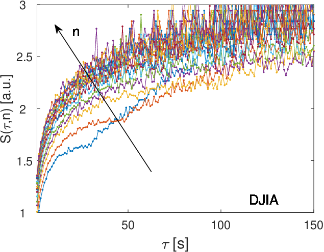
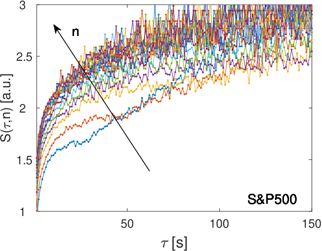
Fig. 1 shows the cluster entropy calculated by using raw data prices. In particular, the plots refer to one month of data (). The series lengths are , and respectively for NASDAQ, DJIA and SP500 as given in Table 2.
Fig. 2 shows the cluster entropy calculated by using raw data prices, as in Fig. 1, but here the series refer to a horizon of twelve months (). The series lengths are , and respectively for NASDAQ, DJIA and SP500 as one can find in the last row of Table 2.
Fig. 3 shows the cluster entropy calculated by using the prices series of the sampled data. The plots refer to the first month of data (). All the series have same length .
Fig. 4 shows the cluster entropy calculated by using the prices series of the sampled data. The plots refer to twelve months (). All the series have same length .
Different curves in each figure correspond to moving average values varying from , , , , up to (with step ).
One can note that the entropy curves exhibit a behaviour consistent with Eq. (10). At small values of the cluster duration , entropy behaves as a logarithmic function. At large values of the cluster duration the curves increase linearly with the term dominating. is -invariant for small values of , while its slope decreases as at larger , as expected according to Eq. (10), meaning that clusters with duration are not power-law correlated, due to the finite-size effects introduced by the partition with window . Hence, they are characterized by a value of the entropy exceeding the curve , which corresponds to power-law correlated clusters. It is worthy to remark that clusters with same duration can be generated by different values of the moving average window . At a constant value of , larger entropy values are obtained as increases.
The entropy of the NASDAQ, DJIA and SP500 prices (shown in Fig. 1, Fig. 2, Fig. 3 and Fig. 4) is representative of a quite general behaviour observed in several markets analysed by using the proposed cluster entropy approach.
In the following, we will discuss how to quantify the horizon dependence of the asset prices by using the cluster entropy function estimated over different periods . To this purpose, we use the cumulative information measure function defined in Eq. (11).
The quantity is calculated by using the values of the entropy of the asset prices estimated over several periods , ranging from one to twelve months, by using raw and sampled data. The first period () of the price sequences is taken in correspondence of January 2018 for all the assets. Multiple period sequences have been built by considering (January and February 2018) and, so on, up to (one year from January to December 2018). Details concerning lengths of the series corresponding to the temporal horizons are reported in Table 2.
The cumulative information measure has been plotted in Fig. 5 for the prices of the NASDAQ, DJIA and SP500. One can observe a dependence of the function at different horizons.
is the same for all implying that the horizon dependence is negligible at small scales (small / small values). Conversely, at large values, i.e. with a broad range of cluster lengths spanning more than one decades of values in the power law distribution, a horizon dependence varying with is found.
For identically distributed sequences of clusters, does not change with regardless of the value of . This, has been shown in Fig. 6 where the cluster entropy of artificially generated series (fractional random walks) are shown. One can note that the curves are practically unchanged at varying horizons and cluster duration . The departure from the iid case can be taken as a measure of price dynamics.
Furthermore, by comparing the figures corresponding to the different assets a dependence of the function is observed. In the case of the NASDAQ the variation seems larger than for the SP500, and even larger than for the DJIA.
5 Discussion and Conclusions
Next, the main results of the analysis of the cluster entropy and the cumulative information measure are compared with the results obtained by using information theoretical approaches by other authors.
To build a cluster entropy index of horizon dependence, i.e. a synthetic numerical parameter with the ability to provide an estimate of the horizon dependence, we consider the entropy integral defined by Eq. (12) at one-period () and at multiples of one period respectively defined as and . The quantity , defined above on the basis of Eq. (12) is called Market Dynamic Index.
To the purpose of comparing our results with those of paper [29], the horizon dependence is calculated as:
| (13) |
Values of Market Dynamic Index and horizon dependence calculated by using the NASDAQ, DJIA and SP500 data are reported in Table 3. The quantity is a reference value of the one-period entropy (lower bound). It is taken as , and respectively for power utility, recursive utility and difference habit agent models of the consumption growth following [29]. The value has been obtained from the curves in Fig. 5 for the prices of the NASDAQ, DJIA and SP500. is the difference between and on account of Eq. (13).
Next, the values of the horizon dependence obtained by using the cluster entropy will be checked against those obtained by using different representative agent models for the definition of the pricing kernel in [29]. The pricing kernel dynamics has been quantified by a measure of entropy dependence on the investment horizon for popular asset pricing models. The pricing kernel accounts for the stochastic dynamic evolution of asset returns, which in their turn contain information about the pricing kernel. The analysis is based on the Kulback-Leibner divergence (also known as relative entropy) of the true probability distribution of the prices with respect to the risk-adjusted probability. On account of those results, it was argued that a realistic asset pricing model should have substantial one-period entropy and modest horizon dependence to justify equity mean excess returns and bond yields at once.
The Kullback-Leibler (KL) divergence of the continuous probability measure with respect to some probability measure , writes:
| (14) |
Eq. (14) can be interpreted as the expectation of the function with respect to the probability :
| (15) |
It can be easily shown that the relative entropy Eq. (14) reduces to Eq. (5) for constant probability .
Investigation of asset price dispersion and dynamics has been put forward by using a variant of the Kullback-Leibler (KL) divergence of the pricing kernels expressed in terms of the ratio between the true and risk-adjusted distribution [29]. In this work, different representative agent models have been considered to quantify the Market Horizon Dependence :
| (16) |
with the quantity defined as:
| (17) |
where is defined as the average of the relative entropy of the pricing kernel, and is calculated at the month . A summary of the horizon dependence obtained by estimating the Kullback-Leibler (KL) entropy with pricing kernels generated by different representative agent models according to the approach of [29] is reported in Table 4.
To further validate the behaviour observed in real-world financial markets, simulations have been performed on artificial data generated by means of the FRACLAB tool available at: https://project.inria.fr/fraclab/. The FRACLAB tool generates Fractional Brownian Motion series with assigned Hurst exponent . The Hurst exponent corresponding to financial prices is generally assumed to be . In Fig. 6, the cluster entropy curve is shown for a FBM series with and different lengths . For the curves shown in Fig. 6 the artificial series has been generated with a total length equal to the one of the NASDAQ index (). Then the artificial series has been divided in twelve consecutive segments with the same lengths of the NASDAQ sub-sequences (values of first column of Table 2). Figures refer respectively to the first segment (), the first sixth segments () and twelve segments ().
To the purpose of fully appreciating the different behaviour of real world market series compared to those exhibited by the artificially generated sequences, the market dynamic index has been calculated for the artificial series (Fig. 7). The Market Dynamic Index has quite a constant value at the different horizons and moving average clusters , thus exhibiting a behaviour different than real market dynamic indexes shown in Fig. 5.
Last but not least, results of statistical significance tests are reported in Table 5. The test has been performed by using the paired t-test to check the null hypothesis that the cluster entropy values obtained on the real-world financial markets and those obtained on the artificial series (FBMs with assumed as benchmark) come from distributions with equal mean and same variance with a probability .
One can note in Table 5 that the probability that the null hypothesis holds true ranges from to . This confirms that the NASDAQ market behaves quite differently from the traditional interpretation of independent elementary stochastic process of price variations, as the FBM with implies. The S&P 500 exhibits an intermediate tendency to behave as ideal market being the probability . The probability for Dow Jones ranges within the interval . Thus it seems that the DJIA index reproduces more closely the behaviour of the fully independent stochastic process involved in the FBM with .
From an economic perspective the results have shown how financial market apparently very similar in terms of regional features, size and volumes may exhibit different horizon dependence. The obtained results are very robust from a statistical point of view. Thus they can represent a valid basis for developing investment tools to quantify risks and extremely useful for investors in classifying markets and choosing their strategy.
References
- [1] Crutchfield JP. Between order and chaos. Nature Physics. 2012;8(1):17–24.
- [2] Bandt C, Pompe B. Permutation entropy: a natural complexity measure for time series. Phys Rev Lett. 2002;88(17):174102.
- [3] Grassberger P, Procaccia I. Characterization of strange attractors. Phys Rev Lett. 1983;50(5):346.
- [4] Marcon E, Scotti I, Hérault B, Rossi V, Lang G. Generalization of the partitioning of Shannon diversity. PLoS ONE. 2014;9(3):e90289.
- [5] Karpiarz M, Fronczak P, Fronczak A. International trade network: fractal properties and globalization puzzle. Phys Rev Lett. 2014;113(24):248701.
- [6] Rubido N, Grebogi C, Baptista MS. Entropy-based generating Markov partitions for complex systems. Chaos: An Interdisciplinary Journal of Nonlinear Science. 2018;28(3):033611.
- [7] Philippatos GC, Wilson CJ. Entropy, market risk, and the selection of efficient portfolios. Applied Economics. 1972;4(3):209–220.
- [8] Fernholz ER. Stochastic portfolio theory. In: Stochastic Portfolio Theory. Springer; 2002. p. 1–24.
- [9] Ou J. Theory of portfolio and risk based on incremental entropy. The Journal of Risk Finance. 2005;6(1):31–39.
- [10] Xu J, Zhou X, Wu DD. Portfolio selection using mean and hybrid entropy. Annals of Operations Research. 2011;185(1):213–229.
- [11] Usta I, Kantar YM. Mean-variance-skewness-entropy measures: a multi-objective approach for portfolio selection. Entropy. 2011;13(1):117–133.
- [12] Zhou R, Wang X, Dong X, Zong Z. Portfolio selection model with the measures of information entropy-incremental entropy-skewness. Advances in Information Sciences and Service Sciences. 2013;5(8):833.
- [13] Zhang WG, Liu YJ, Xu WJ. A possibilistic mean-semivariance-entropy model for multi-period portfolio selection with transaction costs. European Journal of Operational Research. 2012;222(2):341–349.
- [14] Bera AK, Park SY. Optimal portfolio diversification using the maximum entropy principle. Econometric Reviews. 2008;27(4-6):484–512.
- [15] DeMiguel V, Garlappi L, Uppal R. Optimal Versus Naive Diversification: How Inefficient is the Portfolio Strategy? The Review of Financial Studies. 2009;22(5):1915–1953.
- [16] Rödder W, Gartner IR, Rudolph S. An entropy-driven expert system shell applied to portfolio selection. Expert Systems with Applications. 2010;37(12):7509–7520.
- [17] Chandrinos S, Lagaros ND. Construction Of Currency Portfolios By Means Of An Optimized Investment Strategy. Operations Research Perspectives. 2018;.
- [18] Gospodinov N, Maasoumi E, et al. General Aggregation of Misspecified Asset Pricing Models. Federal Reserve Bank of Atlanta; 2017.
- [19] Chen X, Tian Y, Zhao R. Study of the cross-market effects of Brexit based on the improved symbolic transfer entropy GARCH model—An empirical analysis of stock–bond correlations. PLoS ONE. 2017;12(8):e0183194.
- [20] Ormos M, Zibriczky D. Entropy-based financial asset pricing. PLoS ONE. 2014;9(12):e115742.
- [21] Lahmiri S, Bekiros S. The Informational Dynamics of Mean–Variance Relationships in Fertilizer Markets: An Entropic Investigation. Entropy. 2018;20(9):677.
- [22] Lahmiri S. Randomness in denoised stock returns: The case of Moroccan family business companies. Physics Letters A. 2018;382(8):554–560.
- [23] Lahmiri S, Bekiros S, Salvi A. Long-range memory, distributional variation and randomness of bitcoin volatility. Chaos, Solitons & Fractals. 2018;107:43–48.
- [24] Lahmiri S, Bekiros S. Disturbances and complexity in volatility time series. Chaos, solitons & fractals. 2017;105:38–42.
- [25] Lahmiri S, Uddin GS, Bekiros S. Nonlinear dynamics of equity, currency and commodity markets in the aftermath of the global financial crisis. Chaos, solitons & fractals. 2017;103:342–346.
- [26] Hansen LP, Jagannathan R. Implications of Security Market Data for Models of Dynamic Economies. Journal of Political Economy. 1991;99(2):225–262.
- [27] Hansen LP. Nobel Lecture: Uncertainty Outside and Inside Economic Models. Journal of Political Economy. 2014;122(5):945–987. doi:10.1086/678456.
- [28] Hansen LP, Sargent TJ. Macroeconomic Uncertainty Prices. National Bureau of Economic Research; 2019. 25781.
- [29] Backus D, Chernov M, Zin S. Sources of entropy in representative agent models. The Journal of Finance. 2014;69(1):51–99.
- [30] Ghosh A, Julliard C, Taylor AP. What Is the Consumption-CAPM Missing? An Information-Theoretic Framework for the Analysis of Asset Pricing Models. Review of Financial Studies. 2017;30(2):442–504. doi:10.1093/rfs/hhw075.
- [31] Carbone A. Information Measure for Long-Range Correlated Sequences: the Case of the 24 Human Chromosomes. Scientific Reports. 2013;3:2721.
- [32] Carbone A, Stanley HE. Scaling properties and entropy of long-range correlated time series. Physica A: Statistical Mechanics and its Applications. 2007;384(1):21–24.
- [33] Carbone A, Castelli G, Stanley HE. Analysis of clusters formed by the moving average of a long-range correlated time series. Phys Rev E. 2004;69:026105.
- [34] Ponta L, Carbone A, Cincotti S. Detrending Moving Average algorithm: quantifying heterogeneity in financial data. In: Computer Software and Applications Conference (COMPSAC), 2017 IEEE 41st Annual. vol. 2. IEEE; 2017. p. 395–400.
- [35] Ponta L, Carbone A. Information measure for financial time series: Quantifying short-term market heterogeneity. Physica A: Statistical Mechanics and its Applications. 2018;510:132 – 144. doi:https://doi.org/10.1016/j.physa.2018.06.085.
- [36] Shannon CE. A mathematical theory of communication, Part I, Part II. Bell Syst Tech J. 1948;27:623–656.
- [37] Costa M, Goldberger AL, Peng CK. Multiscale entropy analysis of complex physiologic time series. Physical review letters. 2002;89(6):068102.
- [38] Niu H, Wang J. Quantifying complexity of financial short-term time series by composite multiscale entropy measure. Communications in Nonlinear Science and Numerical Simulation. 2015;22(1-3):375–382.
- [39] Humeau-Heurtier A. The multiscale entropy algorithm and its variants: A review. Entropy. 2015;17(5):3110–3123.
| Ticker | Name | Country | Currency | Members | Length |
|---|---|---|---|---|---|
| NASDAQ | Nasdaq Composite | US | USD | 2570 | 6982017 |
| DJIA | Dow Jones Industrial Average | US | USD | 30 | 5749145 |
| SP500 | Standard & Poor 500 | US | USD | 505 | 6142443 |
| Data Length | |||
|---|---|---|---|
| NASDAQ | DJIA | SP500 | |
| 1 | 586866 | 516644 | 516635 |
| 2 | 1117840 | 984101 | 984046 |
| 3 | 1704706 | 1500764 | 1500662 |
| 4 | 2291572 | 1623779 | 2017282 |
| 5 | 2906384 | 2165044 | 2558504 |
| 6 | 3493250 | 2681708 | 3075125 |
| 7 | 4069315 | 3187571 | 3580946 |
| 8 | 4712062 | 3753440 | 4146769 |
| 9 | 5243029 | 4220774 | 4614186 |
| 10 | 5885781 | 4786624 | 5180006 |
| 11 | 6461845 | 5292487 | 5685826 |
| 12 | 6982017 | 5749145 | 6142443 |
| Nasdaq Composite Index (NASDAQ) | ||||
|---|---|---|---|---|
| Entropy Indexes | Power Utility | Recursive Utility | Difference Habit | |
| 30 | 0.0052 | 0.0226 | 0.0208 | |
| 0.0003 | 0.0012 | 0.0011 | ||
| 50 | 0.0052 | 0.0227 | 0.0209 | |
| 0.0003 | 0.0013 | 0.0012 | ||
| 100 | 0.0052 | 0.0229 | 0.0211 | |
| 0.0003 | 0.0015 | 0.0014 | ||
| 150 | 0.0054 | 0.0234 | 0.0215 | |
| 0.0005 | 0.0020 | 0.0018 | ||
| 200 | 0.0056 | 0.0246 | 0.0226 | |
| 0.0007 | 0.0032 | 0.0029 | ||
| Dow Jones Industrial Average Index (DJIA) | ||||
| Entropy Indexes | Power Utility | Recursive Utility | Difference Habit | |
| 30 | 0.0050 | 0.0218 | 0.0201 | |
| 0.0001 | 0.0004 | 0.0004 | ||
| 50 | 0.0050 | 0.0219 | 0.0201 | |
| 0.0001 | 0.0005 | 0.0004 | ||
| 100 | 0.0050 | 0.0217 | 0.0200 | |
| 0.0001 | 0.0003 | 0.0003 | ||
| 150 | 0.0050 | 0.0219 | 0.0201 | |
| 0.0001 | 0.0005 | 0.0004 | ||
| 200 | 0.0050 | 0.0218 | 0.0201 | |
| 0.0001 | 0.0004 | 0.0004 | ||
| S&P 500 Index (SP500) | ||||
| Entropy Indexes | Power Utility | Recursive Utility | Difference Habit | |
| 30 | 0.0051 | 0.0224 | 0.0206 | |
| 0.0002 | 0.0010 | 0.0009 | ||
| 50 | 0.0052 | 0.0226 | 0.0208 | |
| 0.0003 | 0.0012 | 0.0011 | ||
| 100 | 0.0052 | 0.0227 | 0.0209 | |
| 0.0003 | 0.0013 | 0.0012 | ||
| 150 | 0.0052 | 0.0229 | 0.0211 | |
| 0.0003 | 0.0015 | 0.0014 | ||
| 200 | 0.0053 | 0.0230 | 0.0212 | |
| 0.0004 | 0.0016 | 0.0015 | ||
| Constant Variance | ||||
|---|---|---|---|---|
| Entropy | Power Utility | Recursive Utility | Ratio Habit | Difference Habit |
| 0.0049 | 0.0214 | 0.0049 | 0.0197 | |
| 0.0258 | 0.0232 | 0.0003 | 0.0258 | |
| 0.0119 | 0.0011 | -0.0042 | 0.0001 | |
| 0.0208 | 0.0018 | -0.0047 | 0.0061 | |
| Stochastic Variance | ||||
| Entropy | Recursive Utility 1 | Recursive Utility 2 | Campbell Cochrane | - |
| 0.0218 | 0.0249 | 0.0230 | - | |
| 0.0238 | 0.0293 | 0.0230 | - | |
| 0.0012 | 0.0014 | 0 | - | |
| 0.0020 | 0.0044 | 0 | - | |
| with Jumps | ||||
| Entropy | IID w/Jumps | Stochastic Intensity | Constant Intensity 1 | Constant Intensity 2 |
| 0.0485 | 0.0512 | 1.2299 | 0.0193 | |
| 0.0485 | 0.0542 | 15.730 | 0.0200 | |
| 0 | 0.0025 | 9.0900 | 0.0005 | |
| 0 | 0.0030 | 14.5000 | 0.0007 | |
| Probability | |||
|---|---|---|---|
| NASDAQ | DJIA | SP500 | |
| 1 | 0.5154 | 0.8892 | 0.7399 |
| 2 | 0.6026 | 0.9257 | 0.8335 |
| 3 | 0.6470 | 0.9332 | 0.8588 |
| 4 | 0.6631 | 0.9283 | 0.8814 |
| 5 | 0.6823 | 0.9417 | 0.9018 |
| 6 | 0.7124 | 0.9534 | 0.9246 |
| 7 | 0.7162 | 0.9461 | 0.9224 |
| 8 | 0.7288 | 0.9618 | 0.9309 |
| 9 | 0.7370 | 0.9645 | 0.9479 |
| 10 | 0.7409 | 0.9570 | 0.9336 |
| 11 | 0.7542 | 0.9519 | 0.9321 |
| 12 | 0.7584 | 0.9434 | 0.9248 |



Supporting information
This section describes the files available in the Dropbox Shared Folder:
In particular the following items can be found in the dropbox folder:
- •
Data folder
- •
Codes zipped file
DATA
H05Art….zip refers to two data folders. These data can be generated and analysed by using the codes described here below. Horizon.zip contains the horizon (.MAT) data estimated for market series and artificial series shown in Figures 5 and 7. These data have been used to estimate the horizon dependence reported in Table 3. These data have been used to perform the test whose results are reported in Table 5.
CODES
Codes.zip: contains all the MATLAB codes used for the analysis.
The following table provides further details regarding each file included in the Code zipped folder and the algorithm steps.
| List of .m files included in Code.zip | |
|---|---|
| FileName | Description |
| TimeSeriesGenerator.m | generates time series using the FracLab matlab environment. |
| SampledSeries.m | First, creates the data structures. Second it samples the data. It includes the variable “Sampled”. If “Sampled=1” the output data are sampled. If “Sampled=0” the data are raw (i.e. unsampled). |
| Prices.m | It evaluates and saves the prices vector under analysis |
| Entropy.m | evaluates the cluster entropy of the series. It generates the curves plotted in Figures 1, 2, 3, 4 and 6 in the paper. |
| MarketDynamicIndex.m | evaluates the Market Dynamic Index according to Eq. (12). |
| DMIfigure.m | Plots the Market Dynamic Index, i.e. it yields the Figures 5 and 7 in the paper. |
| DMA.m | Function |
| DMAbackward.m | Function |
| DMAcentered.m | Function |
| DMAforward.m | Function |
| ComputeClusterProbability.m | Function |
In Table 7 the main calculation steps are summarized:
- •
Generate the data with the “TimeSeriesGenerator.m” file or use already available timeseries in the specified format.
- •
Create a structured data with option sampled/unsampled the series with the “SampledSeries.m” file.
- •
Create a vector of prices by means of “Prices.m”
- •
Evaluate the entropy by means of “Entropy.m” (to produce Figure 1,2 for unsampled data series; to produce Figure 3 and 4 for sampled data series) .
- •
Evaluate the Market Dynamic Index by means of “MarketDynamicIndex.m”
- •
Plot the MarketDynamic Index by means of “MDIfigure.m” (Figure 5 and Figure 7).
| Workflow of .m files included in Code.zip | ||
|---|---|---|
| FileName | Input files (Data and Functions) | Output files (Data) |
| TimeSeriesGenerator.m | None | Data1.mat, , Data12.mat |
| SampledSeries.m | Data1.mat, , Data12.mat | DataSampled0.mat; DataSampled1.mat |
| Prices.m | DataSampled0.mat, DataSampled1.mat | PricesData1.mat, , PricesData12.mat. |
| Entropy.m | PricesData1.mat, , PricesData12.mat; DMA.m; ComputeClusterProbability.m | SimulationsCompleteData1.mat, SimulationsCompleteData12.mat |
| MarketDynamicIndex.m | SimulationsCompleteData1.mat, SimulationsCompleteData12.mat | MDInPricesData.mat |
| DMIfigure.m | MDInPricesData.mat | None |
| DMA.m | DMAbackward.m; DMAcentered.m; DMAforward.m | None |
| DMAbackward.m | None | None |
| DMAcentered.m | None | None |
| DMAforward.m | None | None |
| ComputeClusterProbability.m | None | None |
Data Availability Statement
Data of NASDAQ, DIJA, SP500 indexes have been downloaded from the Bloomberg terminal: www.bloomberg.com/professional, which is accessible to several organizations worldwide or by activating a subscription via the registration page.
Furthermore we provide a set of series of different lengths (simulating the different horizons) that have been generated artificially by means of the FRACLAB tools freely accessed at: https://project.inria.fr/fraclab/ and a MATLAB code to reproduce the results shown in the Figures.