Graph Neural Networks for Small Graph and Giant Network Representation Learning: An Overview

In IsoNN, the sub-graph based feature extraction process is achieved by a novel graph isomorphic layer. Formally, given a brain graph $G=(\mathcal{V},\mathcal{E})$, its adjacency matrix can be represented as $\mathbf{A}\in\mathbb{R}^{|\mathcal{V}|\times|\mathcal{V}|}$. In order to find the existence of specific sub-graph patterns in the input graph, IsoNN matches the input graph with a set of sub-graph templates. Instead of defining these sub-graph templates manually as the existing works, each template is denoted as a kernel variable $\mathbf{K}_{i}\in\mathbb{R}^{k\times k},\forall i\in\{1,2,\cdots,c\}$ and IsoNN will learn these kernel variables automatically. Here, $k$ denotes the node number in the templates and $c$ is the channel number. Meanwhile, to match one template (i.e., the kernel variable matrix $\mathbf{K}_{i}$) with regions in the input graph (i.e., sub-matrices in $\mathbf{A}$), IsoNN uses a set of permutation matrices, which map both rows and columns of the kernel matrix to the sub-matrices in $\mathbf{A}$ effectively. The permutation matrix can be represented as $\mathbf{P}\in\{0,1\}^{k\times k}$ that shares the same dimensions with the kernel matrix. Given a kernel variable matrix $\mathbf{K}_{i}$ and a regional sub-matrix $\mathbf{M}_{(s,t)}\in\mathbb{R}^{k\times k}$ in $\mathbf{A}$ (where $\mathbf{M}_{(s,t)}(1:k,1:k)=\mathbf{A}(s:s+k-1,t:t+k-1)$ and index pair $s,t\in\{1,2,\cdots,(|\mathcal{V}|-k+1)\}$), there may exist $k!$ different such permutation matrices and the optimal one can be denoted as $\mathbf{P}^{*}$:

where $\mathcal{P}=\{\mathbf{P}_{1},\mathbf{P}_{2},\cdots,\mathbf{P}_{k!}\}$ covers all the potential permutation matrices. The F-norm term measures the mapping loss, which is also used as the graph isomorphic feature in IsoNN. Formally, the isomorphic feature extracted based on the kernel $\mathbf{K}_{i}$ for the regional sub-matrix $\mathbf{M}_{(s,t)}$ in $\mathbf{A}$ can be represented as

where vector $\bar{\mathbf{z}}_{i,(s,t)}\in\mathbb{R}^{k!}$ with $\bar{\mathbf{z}}_{i,(s,t)}(j)=\left\|\mathbf{P}_{j}\mathbf{K}_{i}\mathbf{P}_{j}^{\top}-\mathbf{M}_{(s,t)}\right\|_{F}^{2},\forall j\in\{1,2,\cdots,k!\}$ denoting the features computed on the permutation matrix $\mathbf{P}_{j}\in\mathcal{P}$. Furthermore, by shifting the kernel matrix $\mathbf{K}_{i}$ on regional sub-matrices in $\mathbf{A}$, the isomorphic features extracted by IsoNN from the input graph can be denoted as a 3-way tensor ${\mathcal{Z}}_{i}\in\mathbb{R}^{k!\times(|\mathcal{V}|-k+1)\times(|\mathcal{V}|-k+1)}$, where ${\mathcal{Z}}_{i}(1:k!,s,t)=\bar{\mathbf{z}}_{i,(s,t)}(1:k!)$.

Given a brain graph instance $G_{g}\in\mathcal{B}$ ($\mathcal{B}\subset\mathcal{T}$ denotes the training batch), its extracted isomorphic feature matrix can be denoted as $\mathbf{Q}_{g}$. By feeding its flat vectorized representation vector $\mathbf{q}_{g}=vec(\mathbf{Q}_{g})$ as the input into the classification component (with three fully-connected layers), the predicted label vector by IsoNN on the instance can be represented as $\hat{\mathbf{y}}_{g}$. Several frequently used loss functions, e.g., cross-entropy, can be used to measure the introduced loss between $\hat{\mathbf{y}}_{g}$ and the ground-truth label vector $\mathbf{y}_{g}$. Formally, the fully-connected (FC) layers and the loss function used in IsoNN can be represented as follows:

and

where $\mathbf{W}_{i}$ and $\mathbf{b}_{i}$ are the weight and biase in $i_{th}$ layer, $\sigma(\cdot)$ denotes the sigmoid activation function and $softmax(\cdot)$ is the softmax function for output normalization. Variables $\boldsymbol{\Theta}=(\{\mathbf{K}\}_{i=1}^{k},\{\mathbf{W}_{i},\mathbf{b}_{i}\}_{i=1}^{3})$ (including the kernel matrices and weight/bias terms) involved in the model can be effectively learned with the error back propagation algorithm by minimizing the above loss function. For more information about IsoNN, the readers are suggested to refer to isonn for detailed descriptions.

Given the graph set $\mathcal{G}=\{G_{1},G_{2},\cdots,G_{n}\}$, the goal of graph reordering is to find a node labeling $\ell_{n}$ such that for any two graphs $G_{i},G_{j}\in\mathcal{G}$ randomly draw from $\mathcal{G}$, the expected differences between the distance of the graph connectivity adjacency matrices based on $\ell_{n}$ and the distance of the graphs in the graph space is minimized. Formally, for each graph instance $G_{i}\in\mathcal{G}$, its connectivity adjacency matrix can be denoted as $\mathbf{A}_{i}$. Let $d_{\mathcal{A}}$ and $d_{\mathcal{G}}$ denote the distance metrics on the adjacency matrix domain $\mathcal{A}$ and graph domain $\mathcal{G}$ respectively, the graph reordering problem can be formulated as the following optimization problem:

Graph reordering is a combinatorial optimization problem, which has also be demonstrated to be NP-hard and is computationally infeasible to address in polynomial time. SDBN proposes to apply the spectral clustering to help reorder the nodes and brain graph connectivity instead. Formally, based on the brain graph adjacency matrix $\mathbf{A}_{i}$ of $G_{i}$, its corresponding Laplacian matrix can be represented as $\mathbf{L}_{i}$. The spectral clustering algorithm aims at partitioning the brain graph $G_{i}$ into $K$ modules, where the node-module belonging relationships are denoted by matrix $\mathbf{F}\in\mathbbm{R}^{|\mathcal{V}|\times K}$. The optimal $\mathbf{F}$ can be effectively learned with the following objective function:

where $\mathbf{I}\in\{0,1\}^{K\times K}$ denotes an identity matrix and the constraint is added to ensure one node is assigned to one module only. From the learned optimal $\mathbf{F}$, SDBN can assign the nodes in graph $G_{i}$ to their modules $\mathcal{M}=\{M_{1},M_{2},\cdots,M_{K}\}$, where $\mathcal{V}=\bigcup_{i=1}^{K}M_{i}$ and $M_{i}\cap M_{j}=\emptyset,\forall i\neq j$ and $i,j\in\{1,2,\cdots,K\}$. Such learned modules $\mathcal{M}$ can help reorder the nodes in the graph into relatively compact regions, and the graph connectivity adjacency matrix $\mathbf{A}_{i}$ after reordering can be denoted as $\tilde{\mathbf{A}}_{i}$. Similar operations will be performed on the other graph instances in the set $\mathcal{G}$.

Prior to feeding the reordered graph adjacency matrix to the deep convolutional neural network for representation learning, SDBN proposes to augment the network structure by both refining the connectivity adjacency matrix and creating an additional module identification channel.

• •

  Reordered Adjacency Matrix Refinement: Formally, for graph $G_{i}\in\mathcal{G}$, based on its reordered adjacency matrix $\tilde{\mathbf{A}}_{i}$ obtained from the previous step, SDBN proposes to refine its entry values with the following equation:

  $$\tilde{\mathbf{A}}_{i}(p,q)=\begin{cases}1&\mbox{ for }v_{p},v_{q}\in M_{k},\exists M_{k}\in\mathcal{M};\\ \epsilon&\mbox{ otherwise}.\end{cases}$$

  (9)

  In the equation, term $\epsilon$ denotes a small constant.

• •

  Module Identification Channel Creation: From the reordered adjacency matrix $\tilde{\mathbf{A}}_{i}$ for graph $G_{i}\in\mathcal{G}$, the learned module identity information is actually not preserved. To effectively incorporate such information in the model, SDBN proposes to create one more channel $\mathbf{M}_{i}\in\mathbbm{R}^{|\mathcal{V}|\times|\mathcal{V}|}$ for graph $G_{i}$, whose entry values can be denoted as follows:

  $$\mathbf{M}_{i}(p,q)=\begin{cases}k&\mbox{ for }v_{p},v_{q}\in M_{k},\exists M_{k}\in\mathcal{M};\\ 0&\mbox{ otherwise}.\end{cases}$$

  (10)

Formally, based on the above operations, the inputs for the representation learning component on graph $G_{i}$ will be $\mathbf{X}_{i}=\left[\tilde{\mathbf{A}}_{i};\mathbf{M}_{i}\right]$, which encodes much more information and can help learn more useful representations.

As illustrated in Figure 3, based on the input matrix $\mathbf{X}$ for the graphs in $\mathcal{G}$ (here, the subscript of $\mathbf{X}$ is not indicated and it can represent any graphs in $\mathcal{G}$), SDBN proposes to apply the convolutional neural network for the graph representation learning. To be specific, the convolutional neural network used in SDBN involves two operators: conv and pool, which can be stacked together multiple times to form a deep architecture.

Formally, according to Figure 3, the intermediate representations of the input graphs as well as the corresponding labels in the SDBN can be represented with the following equations:

where $reshape(\cdot)$ flattens the matrix to a matrix and $FC(\cdot)$ denotes the fully-connected layers in the model. In the above equations, $\mathbf{\Theta}$ denotes the involved variables in the model, which will be optimized.

Based on the above model, for all the graph instances $G_{i}\in\mathcal{G}$, we can represent the introduced loss terms by the model as

where $\mathbf{y}_{i}$ and $\hat{\mathbf{y}}_{i}$ represent the ground-truth label vector and the inferred label vector of graph $G_{i}$, respectively.

Meanwhile, in addition to the above loss term, SDBN also incorporates the autoencoder into the model learning process via the depool and deconv operations. The conv and pool operators mentioned above compose the encoder part, whereas the deconv and depool operators will form the decoder part. Formally, based on the learned intermediate representation $\mathbf{X}^{(2)}$ of the input graph matrix $\mathbf{X}$, SDBN computes the recovered representations as follows:

By minimizing the difference between $\hat{\mathbf{X}}^{(1)}$ and ${\mathbf{X}}^{(1)}$, as well as the difference between $\hat{\mathbf{X}}$ and ${\mathbf{X}}$, i.e.,

SDBN can effectively learn the involved variables in the model. As illustrated in Figure 3, the decoder step can work in different manner, which will lead to different regularization terms on the intermediate representations. The performance comparison between IsoNN and SDBN is also reported in isonn, and the readers may refer to isonn; sdbn for more detailed information of the models and the experimental evaluation results.

The LF&ER model works based on the deep autoencoder actually. Autoencoder is an unsupervised neural network model, which projects the instances in original feature representations into a lower-dimensional feature space via a series of non-linear mappings. Figure 4 shows that autoencoder model involves two steps: encode and decode. The encode part projects the original feature vector to the objective feature space, while the decode step recovers the latent feature representation to a reconstruction space. In autoencoder model, we generally need to ensure that the original feature representation of instances should be as similar to the reconstructed feature representation as possible.

Formally, let $\mathbf{x}$ represent the original feature representation of instance $i$, and $\mathbf{y}^{(1)},\mathbf{y}^{(2)},\cdots,\mathbf{y}^{(o)}$ be the latent feature representations of the instance at hidden layers $1,2,\cdots,o$ in the encode step respectively, the encoding result in the objective lower-dimension feature space can be represented as $\mathbf{z}\in\mathbb{R}^{d_{z}}$ with dimension $d_{z}$. Formally, the relationship between these vector variables can be represented with the following equations:

Meanwhile, in the decode step, the input will be the latent feature vector $\mathbf{z}$ (i.e., the output of the encode step), and the final output will be the reconstructed vector $\hat{\mathbf{x}}$. The latent feature vectors at each hidden layers can be represented as $\hat{\mathbf{y}}^{(o)},\hat{\mathbf{y}}^{(o-1)},\cdots,\hat{\mathbf{y}}^{(1)}$. The relationship between these vector variables can be denoted as

In the above equations, $\mathbf{W}$ and $\mathbf{b}$ with different subscripts denote the weight matrices and bias terms to be learned in the model. The objective of the autoencoder model is to minimize the loss between the original feature vector $\mathbf{x}$ and the reconstructed feature vector $\hat{\mathbf{x}}$. Formally, the loss term can be represented as

where $\boldsymbol{\Theta}$ denotes the variables involved in the autoencoder model.

LF&ER proposes to learn the community allocation information for the vibrancy inference and ranking. Formally, spatial structure denotes the distribution of POIs inside the community, e.g., a grocery store lies between two residential buildings; a school is next to the police office. The Spatial structure can hardly be represented with explicit features extracted before, and LF&ER proposes to represent them with a set of latent feature vectors extracted from the geographic distance graph and the mobility connectivity graph defined in the previous subsection. The autoencoder model is applied here for the latent feature extraction.

Autoencoder model has been applied to embed the graph data into lower-dimensional spaces in many of the research works, which will obtain a latent feature representation for the nodes inside the graph. Different from these works, instead of calculating the latent feature for the POI categories inside the communities, LF&ER aims at obtaining the latent feature vector for the whole community, i.e., embedding the graph as one latent feature vector.

As shown in Figure 4, LF&ER transforms the matrix of the graphical distance graph (involving the POI categories) $\mathbf{D}$ into a vector, which can be denoted as

Vector $\mathbf{d}$ will be used as the input feeding into the autoencoder model. The latent embedding feature vector of $\mathbf{d}$ can be represented as $\mathbf{z}_{D}$ (i.e., the vector $\mathbf{z}$ as introduced in the autoencoder model in the previous section), which depicts the layout information of POI categories in the community in terms of the geographical distance. Besides the static layout based on geographic distance graph, the spatial structure of the POIs in the communities can also be revealed indirectly through the human mobility. For a pair of POI categories which are far away geographically, if people like to go between them frequently, it can display another type of structure of the POIs in terms of their functional correlations. Via the multiple fully connected layers, LF&ER will project such learned features to the objective vibrancy scores of the community. We will not introduce the model learning part here, since it also involves the ranking models and explicit feature engineering works, which is not closely related to the topic of this paper. The readers may refer to lfer for detailed description about the model and its learning process. In addition, autoencoder (i.e., the base model of LF&ER) is also compared against IsoNN, whose results are reported in isonn.

Formally, given an input network $G=(\mathcal{V},\mathcal{E})$, its network structure information can be denoted as an adjacency matrix $\mathbf{A}=\{0,1\}^{|\mathcal{V}|\times|\mathcal{V}|}$. The corresponding normalized graph Laplacian matrix can be denoted as $\mathbf{L}=\mathbf{I}-\mathbf{D}^{-\frac{1}{2}}\mathbf{A}\mathbf{D}^{-\frac{1}{2}}=\mathbf{U}\mathbf{\Lambda}\mathbf{U}^{\top}$, where $\mathbf{D}$ is a diagonal matrix with entries $\mathbf{D}(i,i)=\sum_{j}\mathbf{A}(i,j)$ on its diagonal and $\mathbf{I}=diag(\mathbf{1})\in\{0,1\}^{|\mathcal{V}|\times|\mathcal{V}|}$ is an identity matrix with ones on its diagonal. The eigen-decomposition of matrix $\mathbf{L}$ can be denoted as $\mathbf{L}=\mathbf{U}\mathbf{\Lambda}\mathbf{U}^{\top}$, where $\mathbf{U}$ denotes the eigen-vector matrix and diagonal matrix $\mathbf{\Lambda}$ has eigen-values on its diagonal.

The spectral convolution operator defined on network $G$ in GCN is denoted as a multiplication of an input signal vector $\mathbf{x}\in\mathbbm{R}^{d_{x}}$ with a filter $\mathbf{g}_{\boldsymbol{\theta}}=diag(\boldsymbol{\theta})$ (parameterized by variable vector $\boldsymbol{\theta}\in\mathbbm{R}^{d_{\theta}})$ in the Fourier domain as follows:

where notation $\mathbf{U}^{\top}\mathbf{x}$ is defined as the graph Fourier transform of $\mathbf{x}$ and $\mathbf{g}_{\boldsymbol{\theta}}$ can be understood as a function on the eigen-values, i.e., $\mathbf{g}_{\boldsymbol{\theta}}(\mathbf{\Lambda})$.

According to Equ. (19), the computation cost of the term on the right-hand-side will be $\mathcal{O}(|\mathcal{V}|^{2})$. For the giant networks involving millions even billions of nodes, the computation of the graph convolution term will become infeasible, not to mention the eigen-decomposition of the Laplacian matrix $\mathbf{L}$ defined before. Therefore, to resolve such a problem, gcn introduces an approximation of the filter function $\mathbf{g}_{\boldsymbol{\theta}}(\mathbf{\Lambda})$ by a truncated expansion in terms of the Chebyshev polynomial $T_{k}(\cdot)$ up to the $K_{th}$ order as follows:

where $\tilde{\mathbf{L}}=\frac{2}{\lambda_{max}}\mathbf{L}-\mathbf{I}$ and $\lambda_{max}$ is the largest eigen-value in matrix $\mathbf{\Lambda}$. Vector $\boldsymbol{\theta}\in\mathbbm{R}^{k}$ is a vector of Chebyshev coefficients. Noticing that the computational complexity of the term on the right-hand-side is $\mathcal{O}(|\mathcal{E}|)$, i.e., linear in terms of the edge numbers, which will be lower than that of Equ. (19) introduced before.

As proposed in gcn, Equ. (20) can be further simplified by setting $K=1$, $\lambda_{max}=2$, $\boldsymbol{\theta}(0)=-\boldsymbol{\theta}(1)=\theta$, which will reduce the right hand-term of Equ. (20) approximately as follows:

where $\tilde{\mathbf{A}}=\mathbf{A}+\mathbf{I}$ and $\tilde{\mathbf{D}}$ is the diagonal matrix defined on $\tilde{\mathbf{A}}$ instead.

As illustrated in Figure 5, in the case when there exist $C$ input channels, i.e., the input will be a matrix $\mathbf{X}\in\mathbbm{R}^{|\mathcal{V}|\times C}$, and $F$ different filters defined above, the learned graph convolution feature representations will be

where matrix $\hat{\mathbf{A}}=\tilde{\mathbf{D}}^{-\frac{1}{2}}\tilde{\mathbf{A}}\tilde{\mathbf{D}}^{-\frac{1}{2}}$ can be pre-computed in advance. Matrix $\mathbf{W}\in\mathbbm{R}^{C\times F}$ is the filter parameter matrix and $\mathbf{Z}\in\mathbbm{R}^{|\mathcal{V}|\times F}$ will be the learned convolved representations of all the nodes. The computational time complexity of the operation will be $\mathcal{O}(|\mathcal{E}|FC)$.

The GCN model can have a deeper architecture by involving multiple graph convolution operators defined in the previous sections. For instance, the GCN model with two layers can be represented with the following equations:

In the above equation, matrices $\mathbf{W}_{1}$ and $\mathbf{W}_{2}$ are the involved variables in the model. ReLU is used as the activation function for the hidden layer 1, and softmax function is used for the output result normalization. By comparing the inferred labels, i.e., $\hat{\mathbf{Y}}$, of the labeled instances against their ground-truth labels, i.e., ${\mathbf{Y}}$, the model variables can be effectively learned by minimizing the following loss function:

where $\boldsymbol{\Theta}$ covers all the variables in the model.

For representation simplicity, node subscript is used as its corresponding index in the label matrix $\mathbf{Y}$. Notation $d_{y}$ denotes the number of labels in the studied problem, and $d_{y}=2$ for the traditional binary classification tasks. The readers can also refer to gcn for detailed information of the GCN model.

Formally, given an input network $G=(\mathcal{V},\mathcal{E})$ and the raw features of the nodes, the node features can be denoted as a matrix $\mathbf{X}\in\mathbbm{R}^{|\mathcal{V}|\times d_{x}}$, where $d_{x}$ denotes the dimension of the node feature vectors. Furthermore, for node $v_{i}\in\mathcal{V}$, its feature vector can also be represented as $\mathbf{x}_{i}=\mathbf{X}(i,:)$ for simplicity. Without considerations about the network structures, via a mapping matrix $\mathbf{W}\in\mathbbm{R}^{d_{x}\times d_{h}}$, the nodes can be projected to their representations in the hidden layer. Meanwhile, to further incorporate the network structure information into the model, based on the network structure, the neighbor set of node $v_{i}$ can be denoted as $\Gamma(v_{i})=\{v_{j}|v_{j}\in\mathcal{V}\land(v_{i},v_{j})\in\mathcal{E}\}\cup\{v_{i}\}$, where $\{v_{i}\}$ is also added and treated as the self-neighbor. As illustrated in Figure 6, GAT proposes to compute the attention coefficient between nodes $v_{i}$ and $v_{j}$ (if $v_{j}\in\Gamma(v_{i}$)) as follows:

where $\mathbf{a}\in\mathbbm{R}^{2d_{h}}$ is a variable vector for weighted sum of the entries in vector $\mathbf{W}\mathbf{x}_{i}\sqcup\mathbf{W}\mathbf{x}_{j}$ and $\sqcup$ denotes the concatenation operator of two vectors. LeakyReLU function is added here mainly for the model learning considerations.

To further normalize the coefficients among all the neighbors, GAT further adopts the softmax function based on the coefficients defined above. Formally, the final computed weight between nodes $v_{i}$ and $v_{j}$ can be denoted as

GAT effectively update the nodes’ representations by aggregating the information from their neighbors (including the self-neighbor). Formally, the learned hidden representation of node $v_{i}$ can be represented as

GAT can be in a deeper architecture by involving multiple attentive node representation updating. In the deep architecture, for the upper layers, the representation vector $\mathbf{h}_{i}$ will be treated as the inputs feature vector instead, and we will not over-elaborate that here.

As introduced in gat, to stabilize the learning process of the model, GAT can be further extended to include the multi-head attention as illustrated in Figure 6. Specifically, let $K$ denote the number of involved attention mechanisms. Based on each attention mechanism, the learned representations of node $v_{i}$ based on the above descriptions (i.e., Equ. (27)) can be denoted as $\mathbf{h}_{i}^{(1)}$, $\mathbf{h}_{i}^{(2)}$, $\cdots$, $\mathbf{h}_{i}^{(K)}$, respectively. By further aggregating such learned representations together, the ultimate learned representation of node $v_{i}$ can be denoted as

Several different aggregation function is tried in gat, including concatenation and average:

• •

  Concatenation:

  $$\mathbf{h}_{i}^{\prime}=\bigsqcup_{k=1}^{K}\sigma\left(\sum_{v_{j}\in\Gamma(v_{i})}\alpha^{(k)}_{i,j}\mathbf{W}^{(k)}\mathbf{x}_{j}\right).$$

  (29)

• •

  Average:

  $$\mathbf{h}_{i}^{\prime}=\sigma\left(\frac{1}{K}\sum_{k=1}^{K}\sum_{v_{j}\in\Gamma(v_{i})}\alpha^{(k)}_{i,j}\mathbf{W}^{(k)}\mathbf{x}_{j}\right).$$

  (30)

The learning process of the GAT model is very similar to that of GCN introduced in Section 3.1.3, and we will not introduce that part again here. The readers can also refer to gat for more detailed descriptions about the model as well as its experimental performance.

Given a heterogeneous input network $G=(\mathcal{V},\mathcal{E})$, the node set $\mathcal{V}$ in the network can be divided into multiple subsets depending on their node types. It is similar for the links in set $\mathcal{E}$. Here, for the representation simplicity, we will follow the news augmented heterogeneous social network example illustrated in dif when introducing the model. As illustrated in Figure 8, there exist three different types of nodes (i.e., creator, news article and subject) and two different types of links (i.e., the creator-article link and article-subject link) in the network. Formally, the node set can be categories into three subsets, i.e., $\mathcal{V}=\mathcal{U}\cup\mathcal{N}\cup\mathcal{S}$, and the link set can be categorized into two subsets, i.e., $\mathcal{E}=\mathcal{E}_{u,n}\cup\mathcal{E}_{n,s}$.

For each node in the network, e.g., $v_{i}\in\mathcal{V}$, its extracted raw feature vector can be denoted as $\mathbf{x}_{i}$. As introduced at the beginning of Section 3, in many cases, the network is partially labeled. Formally, the label vector of node $v_{i}$ is represented as $\mathbf{y}_{i}$. For each nodes in the input network, DifNN utilizes one GDU (which will be introduced in the following subsection) to model its representations and the connections with other neighboring nodes. For instance, based on the input network in Figure 8, its corresponding DifNN model architecture can be represented in Figure 8. Via the gdu neuron unit, DifNN can effectively project the node inputs to their corresponding labels. The parameters involved in the DifNN model can be effectively trained based on the labeled nodes via the back propagation algorithm. In the following two subsections, we will introduce the detailed information about GDU as well as the DifNN model training.

To introduce the GDU neuron, we can take news article nodes as an example here. Formally, among all the inputs of the GDU model, $\mathbf{x}_{i}$ denotes the extracted feature vector for news articles, $\mathbf{z}_{i}$ represents the input from other GDUs corresponding to subjects, and $\mathbf{t}_{i}$ represents the input from other GDUs about creators. Considering that the GDU for each news article may be connected to multiple GDUs of subjects and creators, the $mean(\cdot)$ of the outputs from the GDUs corresponding to these subjects and creators will be computed as the inputs $\mathbf{z}_{i}$ and $\mathbf{t}_{i}$ instead respectively, which is also indicated by the GDU architecture illustrated in Figure 9. For the inputs from the subjects, GDU has a gate called the “forget gate”, which may update some content of $\mathbf{z}_{i}$ to forget. The forget gate is important, since in the real world, different news articles may focus on different aspects about the subjects and “forgetting” part of the input from the subjects is necessary in modeling. Formally, the “forget gate” together with the updated input can be represented as

Here, operator $\otimes$ denotes the entry-wise product of vectors and $\mathbf{W}_{f}$ represents the variable of the forget gate in GDU.

Meanwhile, for the input from the creator nodes, a new node-type “adjust gate” is introduced in GDU. Here, the term “adjust” models the necessary changes of information between different node categories (e.g., from creators to articles). Formally, the “adjust gate” as well as the updated input can be denoted as

where $\mathbf{W}_{e}$ denotes the variable matrix in the adjust gate.

GDU allows different combinations of these input/state vectors, which are controlled by the selection gates $\mathbf{g}_{i}$ and $\mathbf{r}_{i}$ respectively. Formally, the final output of GDU will be

where $\mathbf{g}_{i}=\sigma(\mathbf{W}_{g}\left[\mathbf{x}_{i}^{\top},\mathbf{z}_{i}^{\top},\mathbf{t}_{i}^{\top}\right]^{\top})$, and $\mathbf{r}_{i}=\sigma(\mathbf{W}_{r}\left[\mathbf{x}_{i}^{\top},\mathbf{z}_{i}^{\top},\mathbf{t}_{i}^{\top}\right]^{\top})$, and term $\mathbf{1}$ denotes a vector filled with value $1$. Operators $\oplus$ and $\ominus$ denote the entry-wise addition and minus operation of vectors. Matrices $\mathbf{W}_{u}$, $\mathbf{W}_{g}$, $\mathbf{W}_{r}$ represent the variables involved in the components. Vector $\mathbf{h}_{i}$ will be the output of the GDU model.

The introduced GDU model also works for both the news subjects and creator nodes in the network. When applying the GDU to model the states of the subject/creator nodes with two input only, the remaining input port can be assigned with a default value (usually vector $\mathbf{0}$). In the following section, we will introduce how to learn the parameters involved in the DifNN model for concurrent inference of multiple nodes.

In the DifNN model as shown in Figure 8, based on the output state vectors of news articles, news creators and news subjects, the framework will project the feature vectors to their labels. Formally, given the state vectors $\mathbf{h}_{n,i}$ of news article $n_{i}$, $\mathbf{h}_{u,j}$ of news creator $u_{j}$, and $\mathbf{h}_{s,l}$ of news subject $s_{l}$, their inferred labels can be denoted as vectors $\mathbf{y}_{n,i},\mathbf{y}_{u,j},\mathbf{y}_{s,l}\in\mathcal{R}^{|\mathcal{Y}|}$ respectively, which can be represented as

where $\mathbf{W}_{u}$, $\mathbf{W}_{n}$ and $\mathbf{W}_{s}$ define the weight variables projecting state vectors to the output vectors.

Meanwhile, based on the news articles in the training set $\mathcal{T}_{n}\subset\mathcal{N}$ with the ground-truth label vectors $\{\hat{\mathbf{y}}_{n,i}\}_{n_{i}\in\mathcal{T}_{n}}$, the loss function of the framework for news article label learning are defined as the cross-entropy between the prediction results and the ground truth:

Similarly, the loss terms introduced by news creators and subjects based on training sets $\mathcal{T}_{u}\subset\mathcal{U}$ and $\mathcal{T}_{s}\subset\mathcal{S}$ can be denoted as

where $\mathbf{y}_{u,j}$ and $\hat{\mathbf{y}}_{u,j}$ (and $\mathbf{y}_{s,l}$ and $\hat{\mathbf{y}}_{s,l}$) denote the prediction result vector and ground-truth vector of creator (and subject) respectively.

Formally, the main objective function of the DifNN model can be represented as follows:

where $\mathbf{\Theta}$ denotes all the involved variables to be learned, term ${reg}(\mathbf{\Theta})$ represents the regularization term (i.e., the sum of $L_{2}$ norm on the variable vectors and matrices), and $\alpha$ denotes the regularization term weight. By resolving the optimization functions, variables in the model can be effectively learned with the back-propagation algorithm. For the news articles, creators and subjects in the testing set, their predicted labels will be outputted as the final result.

GNL also adopts GDU as the basic neuron unit and extends it to the dynamic network regression problem settings, which can model both the network snapshot internal connections and the temporal dependency relationships between sequential network snapshots for the nodes.

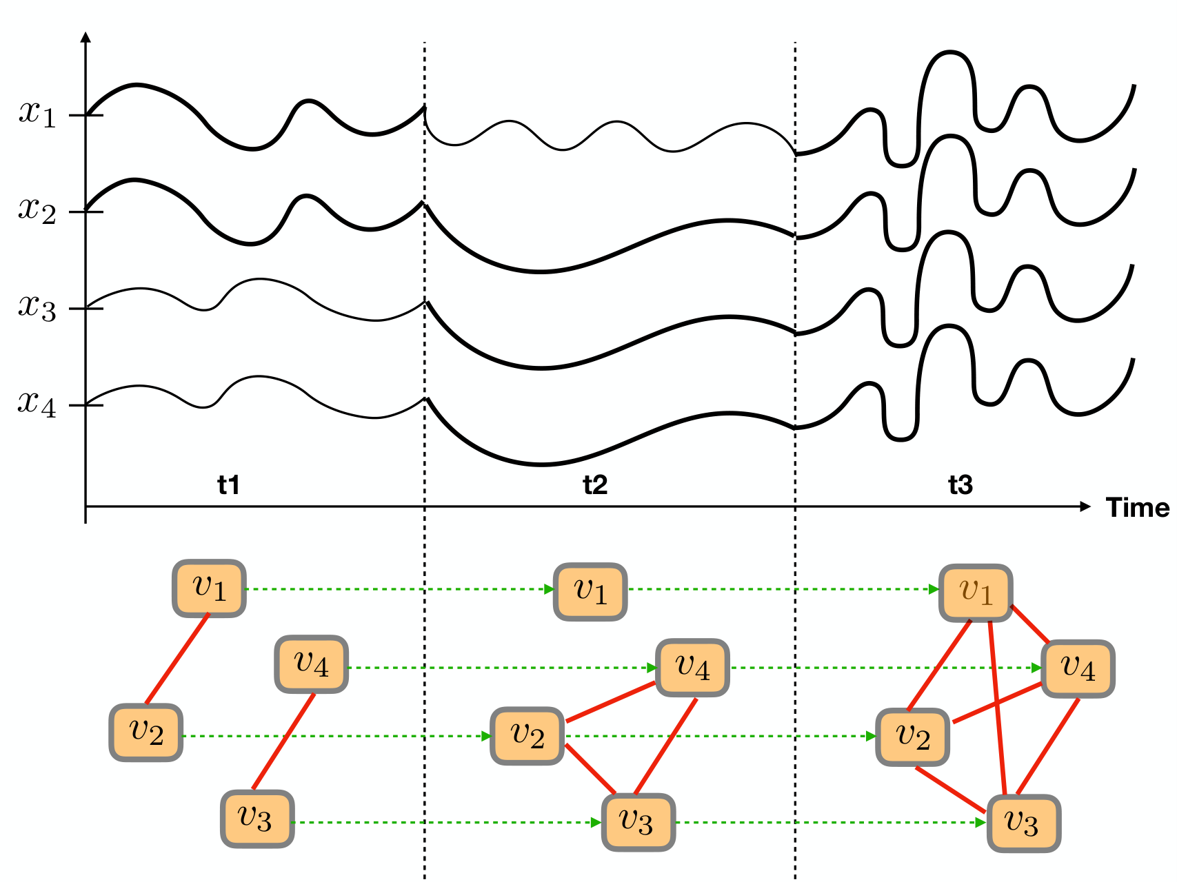
Formally, given the time series data about a set of connected entities, such data can be represented as a dynamic network set $\mathcal{G}=\{G^{(1)},G^{(2)},\cdots,G^{(t)}\}$, where $t$ denotes the maximum timestamp. For each network $G^{(\tau)}\in\mathcal{G}$, it can be denoted as $G^{(\tau)}=(\mathcal{V}^{(\tau)},\mathcal{E}^{(\tau)})$ involving the node set $\mathcal{V}^{(\tau)}$ and link set $\mathcal{E}^{(\tau)}$, respectively. Given a node $v_{i}$ in network $G^{(\tau)}$, its in-neighbors and out-neighbors in the network can be denoted as sets $\Gamma_{in}(v_{i})=\{v_{j}|v_{j}\in\mathcal{V}^{(\tau)}\land(v_{j},v_{i})\in\mathcal{E}^{(\tau)}\}$ and $\Gamma_{out}(v_{i})=\{v_{j}|v_{j}\in\mathcal{V}^{(\tau)}\land(v_{i},v_{j})\in\mathcal{E}^{(\tau)}\}$. Here, the link direction denotes the influences among the nodes. If the influences in the studied networks are bi-directional, the in/out neighbor sets will be identical, i.e., $\Gamma_{in}(v_{i})=\Gamma_{out}(v_{i})$.

For node $v_{i}$ in network $G^{(\tau)}$ of the $\tau_{th}$ timestamp, the input attribute values of $v_{i}$ can be denoted as an input feature vector $\mathbf{x}_{i}^{(\tau)}\in\mathbbm{R}^{d_{x}}$. GDU maintains a hidden state vector for each node, and the vector of node $v_{i}$ at timestamp $\tau$ can be denoted as $\mathbf{h}_{i}^{(\tau)}\in\mathbbm{R}^{d_{h}}$. As illustrated in Figure 11, besides the feature vector $\mathbf{x}_{i}^{(\tau)}$ and hidden state vector $\mathbf{h}_{i}^{(\tau)}$ inputs, the GDU neuron of $v_{i}$ will also accept the inputs from $v_{i}$’s input neighbor nodes, i.e., $\{\mathbf{h}_{j}^{(\tau)}\}_{v_{j}\in\Gamma_{in}(v_{i})}$, which will be integrated via certain aggregation operators:

The $\mbox{Aggregate}(\cdot)$ operator used in GNL will be introduced in detail in the next subsection.

A common problem with existing graph neural network models is over-smoothing, which will reduce all the nodes in the network to similar hidden representations. Such a problem will be much more serious when the model involves a deep architecture with multiple layers. To resolve such a problem, besides the attention mechanism to be introduced later, GDU introduces several gates for the neural state adjustment as introduced in Section 3.3.2. Formally, based on the input vectors $\mathbf{x}_{i}^{(\tau)}$, $\mathbf{z}_{i}^{(\tau)}$ and $\mathbf{h}_{i}^{(\tau)}$, the representation of node $v_{i}$ in the next timestamp $\tau+1$ can be represented as

The concrete representation of the $GDU(\cdot)$ function is similar to Equ. (31)-(33) introduced before, and $\mathbf{\Theta}$ denotes the variables involved in the GDU neuron.

In this part, we will introduce the $\mbox{Aggregate}(\cdot)$ operator used in Equ. (39) for node neighborhood influence integration proposed in gnl. The GNL model defines such an operator based on an attention mechanism. Formally, given the node $v_{i}$ and its in-neighbor set $\Gamma_{in}(v_{i})$, for any node $v_{j}\in\Gamma_{in}(v_{i})$, GNL quantifies the influence coefficient of $v_{j}$ on $v_{i}$ based on their hidden state vectors $\mathbf{h}_{j}^{(\tau)}$ and $\mathbf{h}_{i}^{(\tau)}$ as follows:

In the above equation, operator $\mbox{Linear}(\cdot;\mathbf{w}_{a})$ denotes a linear sum of the input vector parameterized by weight vector $\mathbf{w}_{a}$. According to gat, out of the model learning concerns, the above influence coefficient term can be slightly changed by adding the LeakyReLU function into its definition. Formally, the final influence coefficient used in GNL is represented as follows:

References

- [1] Yixin Chen, Lin Meng, and Jiawei Zhang. Graph neural lasso for dynamic network regression. CoRR, abs/1907.11114, 2019.
- [2] William L. Hamilton, Rex Ying, and Jure Leskovec. Inductive representation learning on large graphs. CoRR, abs/1706.02216, 2017.
- [3] Thomas N. Kipf and Max Welling. Semi-supervised classification with graph convolutional networks. CoRR, abs/1609.02907, 2016.
- [4] Lin Meng and Jiawei Zhang. Isonn: Isomorphic neural network for graph representation learning and classification. CoRR, abs/1907.09495, 2019.
- [5] Petar Veličković, Guillem Cucurull, Arantxa Casanova, Adriana Romero, Pietro Liò, and Yoshua Bengio. Graph Attention Networks. International Conference on Learning Representations, 2018.
- [6] Pengyang Wang, Jiawei Zhang, Guannan Liu, Yanjie Fu, and Charu Aggarwal. Ensemble-Spotting: Ranking Urban Vibrancy via POI Embedding with Multi-view Spatial Graphs, pages 351–359.
- [7] Shen Wang, Lifang He, Bokai Cao, Chun-Ta Lu, Philip S. Yu, and Ann B. Ragin. Structural deep brain network mining. In Proceedings of the 23rd ACM SIGKDD International Conference on Knowledge Discovery and Data Mining, KDD ’17, pages 475–484, New York, NY, USA, 2017. ACM.
- [8] Jiawei Zhang, Limeng Cui, Yanjie Fu, and Fisher B. Gouza. Fake news detection with deep diffusive network model. CoRR, abs/1805.08751, 2018.
- [9] Jiawei Zhang, Limeng Cui, and Fisher B. Gouza. SEGEN: sample-ensemble genetic evolutional network model. CoRR, abs/1803.08631, 2018.