Quantum light-matter interaction and controlled phonon scattering in a photonic Fano cavity
Abstract
The Fano effect arises from the interference between a continuum of propagating modes and a localised resonance. By using this resonance as one of the mirrors in an optical cavity, a localised mode with a highly asymmetric line shape is obtained. Placing a single quantum emitter inside the cavity leads to a new regime of cavity quantum electrodynamics, where the light–matter interaction dynamics is fundamentally different from that observed in a conventional cavity with Lorenztian lineshape. Furthermore, when the vibrational dynamics of the emitter is taken into account, an intricate phonon–photon interplay arises, and the optical interference induced by the Fano mirror significantly alters the leakage of energy into vibrational modes. We demonstrate that this control mechanism improves the maximum attainable indistinguishability of emitted photons, as compared to an equivalent cavity with a conventional mirror.
The Fano effect arises from the interference between a continuum of modes and a localised resonance Fano 1961. A photonic variant of the phenomenon can be realised by placing a nanocavity close to a waveguide with a partially transmitting element, as shown in Fig. 1a. In this configuration, photons in the waveguide can propagate directly through the partially transmitting element or via the cavity. The resulting interference leads to a strong and asymmetric frequency dependence of the transmittivity through the system Heuck et al. 2013 (see Fig. 1b). By replacing one of the mirrors in a conventional Fabry-Pérot cavity with such a Fano mirror, one may construct an exotic nanophotonic structure – a so-called Fano cavity. The interference between the two dissipation paths of the Fano mirror leads to a quasi-localised cavity mode with an asymmetric line-shape that is far from a Lorentzian Fabry-Pérot cavity. Indeed, in the limit where the two paths exhibit perfect destructive interference, this mode becomes a true bound state in the continuum Friedrich and Wintgen 1985, which has recently been studied with a non-linear atomic mirror that allows for excitation of the bound mode through a two-photon process Cotrufo and Alù 2019; Calajó et al. 2019. Such Fano cavities are of growing interest in the field of integrated nanophotonics, where Fano lasers with unique dynamics Yu et al. 2017; Mork et al. 2014 and non-reciprocal elements Yu et al. 2015 have been demonstrated. However, there are a number of open questions regarding how the non-Lorentzian nature of the cavity will impact the emission properties of a single quantum emitter.
In this paper, we extend the description of a Fano cavity into the regime of cavity quantum electrodynamics (cQED), where we consider a single solid-state emitter placed in the centre of the cavity. This theory allows us to directly investigate the impact that the non-Lorentzian lineshape of the Fano cavity has on the optical properties of the emitter, and crucially demonstrate that the coupling between a solid-state emitter and its vibrational environment can be engineered by structuring the optical local density of states (LDOS). This effect is observed through drastic modifications to the phonon sideband present in solid-state emitters Besombes et al. 2001, which we show becomes highly sensitive to the shape of the LDOS of the nanophotonic structure, and is able to suppress phonon emission (see Fig. 1c), resulting in photon indistinguishabilities that surpass standard Lorentzian cavities.
When studying light-matter coupling in cQED, quantisation of the cavity mode is of paramount importance. Therefore, a central question in the analysis of the Fano cavity is how to fully represent the structured LDOS in regimes of potentially strong light-matter coupling. Recently, a general quantisation scheme based on symmetrised quasi-normal modes has been presented, which relies on a numerical calculation of the electromagnetic modes of the system Franke et al. 2019. In contrast, we make use of a simple and intuitive approach that provides an analytical expression for the LDOS of the Fano cavity. We then develop a mapping that extracts the key features of the LDOS and incorporates them into an enlarged system Hamiltonian. This mapping generates a pair of dissipative bosonic modes (see Fig. 1d) which are coupled in order to capture the predominant interference pathways, and thus the non-Lorentzian behaviour of the Fano cavity. Resolving such interference features requires at least two coupled modes, and thus cannot be analysed with any single-mode mapping technique such as the reaction coordinate master equations Iles-Smith et al. 2014; Iles-Smith et al. 2016. Our two-mode representation allows us to fully account for strong-coupling effects between the emitter and the Fano cavity, while simultaneously capturing the non-Markovian dynamics arising from interactions with the vibrational phonon environment of the host lattice Roy-Choudhury and Hughes 2015a; Iles-Smith et al. 2017.
In the rotating wave approximation, the Hamiltonian describing the interaction between a single two level emitter and the electromagnetic field is , where is the bosonic annihilation operator for the -mode of the field, is the emitter transition operator between the excited () and ground () states, and is the coupling constant. The spectral density, , with the frequency of the mode, then fully characterises the interaction. This spectral density is equivalent to the LDOS of the electromagnetic field Lodahl et al. 2015, which can be calculated using an extension of Refs. Gregersen et al. 2016; Rybin et al. 2016; Denning et al. 2018 where the right mirror is a Fano mirror with reflectivity Yoon and Magnusson 2013; Heuck et al. 2013; Yu et al. 2015. Here, is the bare reflectivity of the partially transmitting element in the waveguide; is the coupling rate between the nanocavity and the waveguide, which is taken equal on both sides of the cavity; is the intrinsic loss rate of the nanocavity; is the total loss rate; is the resonant frequency of the nanocavity and is the parity () of the Fano mirror, determining whether the reflectivity minimum is on the blue- or red-detuned side of the maximum Osterkryger et al. 2016; Heuck et al. 2013. When the emitter is placed in the middle of the cavity, the LDOS becomes sup
| (1) |
where is the spontaneous emission into the bare waveguide in the absence of mirrors, is the reflectivity of the conventional left mirror (here taken to be ) and is the free spectral range of the bare resonator set by , with the speed of light, the effective waveguide group index and the cavity length. The interplay between the roundtrip phase in the cavity and the reflection phase of the Fano mirror gives rise to a resonance and an anti-resonance appearing as a peak and a dip in the LDOS (see Fig. 2a). Fig. 2b shows how the LDOS depends on frequency and the coupling rate between the nanocavity and the waveguide. At the critical point where the anti-resonance crosses over from the red-detuned to the blue-detuned side of the resonance, the peak corresponds to a bound state in the continuum Friedrich and Wintgen 1985. At this point, the lifetime of this bound state is only limited by the intrinsic losses of the nanocavity.
Various techniques have been developed to perform the non-trivial task of constructing an accurate representation of a continuous bosonic environment in terms of a set of discrete modes. Reaction coordinate master equations have previously been used to extract a single damped bosonic mode from a continuous reservoir Iles-Smith et al. 2014; Iles-Smith et al. 2016. Such a representation, however, has so far only been successful in representing environments that are Lorentzian in nature, and therefore cannot capture the central features of the Fano cavity induced by interference. The pseudomode mapping associates a discrete mode with each complex pole of the spectral density Garraway 1997; Dalton et al. 2001; Mazzola et al. 2009. This technique is exact but requires that all poles in the spectral density are included in the mapping, because the sum of the residues must have a vanishing real part. In the present paper, the spectral density has infinitely many poles, and therefore such an approach is infeasible. A more flexible approach allows representation of a bosonic environment as an infinite discrete chain of coupled harmonic oscillators Chin et al. 2010, with the possibility of truncating the chain after a finite number of links Woods et al. 2014. In order to be efficient, the chain needs to represent the spectral density accurately with only a few links, or rely on sophisticated numerical techniques to calculate the dynamics of the reduced system Prior et al. 2010; Rosenbach et al. 2016. However, we have found that for the Fano cavity, no clear convergence within 10 chain sites is observable. This is largely attributed to the interference between the two optical decay paths in the physical structure that generates the central features of the spectral density, which is challenging to reproduce in an equivalent one-dimensional system.
On a more general note, it was recently shown that the reduced dynamics of a quantum system, , with a bosonic environment, , is invariant under a substitution of by a different bosonic environment, , provided that the spectral densities of and are equal Tamascelli et al. 2018. In most practical applications, the correspondence between the spectral densities of and cannot be exact, but their difference within a relevant frequency range determined by serves as a measure for equivalence of a given mapping. This strategy can be exemplified by the canonical representation of a QED emitter–cavity system by the dissipative Jaynes-Cummings model, where the cavity is described by a single mode with a finite lifetime. To describe the asymmetric Fano cavity mode, it is necessary to use two modes (see Fig. 1d), with annihilation operators where light-matter coupling is described by the master equation
| (2) |
Here, is the free evolution Hamiltonian of the emitter, is the Lindblad dissipator and
| (3) |
We have introduced the emitter-cavity coupling strength , the resonant frequency and leakage rate for the -cavity mode, and the intercavity coupling strength . The interference between the two modes appearing in the dissipator is crucial for capturing the underlying physical interference between the direct and cavity-mediated transmissions in the Fano mirror.
To establish a link between the microscopic physical parameters of the cavity and the parameters in the discrete representation, we calculate the spectral density generated by the -modes and compare it to the LDOS of Eq. (1) to minimise the error, , over a finite frequency window, , around the emitter resonance. The spectral density of the discrete mode representation is calculated as , where denotes the free evolution of the cavity modes under Eq. (2) in the absence of the emitter. With analytic expressions for and , we require that the position of the complex poles of is equal to those of , and the imaginary part of the sum of the residues are equal sup. These requirements determine five out of the seven parameters in the discrete-mode representation. The remaining two parameters are determined numerically by minimising . The LDOS in Eq. (1) features an infinite number of discrete poles corresponding to the Fabry-Pérot resonances. However, the emitter is only sensitive to the the LDOS in the vicinity of its resonance frequency. For cavities with length scales of a few micrometers, the free spectral range is much larger than any features in the spectral response of the emitter and phonon modes, covering a few meV. As such, we find that features of the bound mode in the Fano cavity are very well described by two nearby poles of , separated from the remaining poles by . In Fig. 2a, we provide an example of how the mapped spectral density, , (green dashed line and shaded area) reproduces with a high precision the LDOS, (black solid line). A recent related work presents a similar technique based on a numerical search for the optimal parameters for a coupled network of harmonic oscillators to represent a given spectral density Mascherpa et al. 2019.
Interactions with longitudinal acoustic phonons are described by the additional Hamiltonians and Wilson-Rae and Imamoğlu 2002; Mahan 2013; Kaer and Mørk 2014. The phonon interactions are characterised by the spectral density , with overall coupling strength and cutoff frequency Nazir 2008; Nazir and McCutcheon 2016. To account for the non-Markovian emitter–phonon correlations, we use the polaron transformation Wilson-Rae and Imamoğlu 2002; Iles-Smith et al. 2017; Nazir and McCutcheon 2016; McCutcheon and Nazir 2010; Roy-Choudhury and Hughes 2015a to derive a master equation sup. The resulting master equation is a modification of Eq. (2) in which the light–matter coupling rate, , is effectively reduced and an additional dissipator is introduced. We furthermore add a dissipator accounting for spontaneous emission into the radiation modes, McCutcheon and Nazir 2013; Roy-Choudhury and Hughes 2015b.
The photon indistinguishability is an important feature that characterises the coherence properties of the light emitted from a cQED system Iles-Smith et al. 2017; Roy-Choudhury and Hughes 2015a; Kaer et al. 2010; Kaer and Mørk 2014; Hornecker et al. 2017. In the present situation, the indistinguishability reveals how strongly the photonic structure is able to modify the phonon dynamics by shaping the phonon sideband or enhancing/suppressing the zero phonon line. Here, the emission from the system is studied by choosing an initial state where the emitter is excited and the electromagnetic field is in the vacuum state, and then calculating the optical spectrum as the system relaxes and a single photon is emitted. Of particular interest is the two-colour spectrum of light emitted from the system through the Fano mirror, Iles-Smith et al. 2017, which is related to the dipole spectrum, , through the optical Green’s function as , where and is the transmittivity of the Fano mirror. This two-colour spectrum is related to the observable emission spectrum, , as . Furthermore, it allows calculation of photon indistinguishability as sup; Iles-Smith et al. 2017; Denning et al. 2018
| (4) |
where is the emitted energy into the detection channel. In a multiphoton experiment with subsequent two-photon interference events, the accumulated visibility scales as , where is the distinguishibility, which quantifies the decoherence-induced error Kiraz et al. 2004.
Fig. 3a shows the photon indistinguishability as a function of nanocavity coupling rate and emitter transition frequency, corresponding to parameter variations over the LDOS shown in Fig. 2b. The behaviour of the indistinguishability over the parameter space shows a rich structure, which is mainly a result of the interplay between the electromagnetic LDOS and the phonon sideband. Along the dotted line, the emitter transition frequency is tuned to the resonance of the Fano cavity, meaning that emission is funnelled into the zero-phonon line. In the lower part of the plot, the LDOS anti-resonance is located on the red-detuned side of the resonance and thereby suppresses emission into the phonon sideband while enhancing emission into the zero phonon line. The combination of these effects leads to a minimal distinguishability of 0.010 (indicated with a white dot). The emission spectrum corresponding to these parameters is shown in Fig. 3b (solid orange; shading). To understand how this spectrum arises, the bulk emission spectrum is indicated (thin blue) along with the electromagnetic LDOS (grey dashed). This demonstrates how the anti-resonance leads to a spectral hole in the phonon sideband. In the supplemental material sup, we show that the minimal attainable distinguishability for the same optical structure with a conventional mirror is Iles-Smith et al. 2017; Denning et al. 2018, found when the mirror reflectivity is optimised to . Fig. 3c shows the emission spectrum for parameters corresponding to the black dot in Fig. 3a, where the cavity lifetime is long enough for the system to enter the strong coupling regime and two polariton peaks can be seen along with the spectral hole in the phonon sideband. In this regime, phonons reduce the indistinguishability by driving transitions between the polaritons Kaer et al. 2010; Kaer and Mørk 2014; Iles-Smith et al. 2017. If the emitter frequency is blue-shifted relative to the resonance line in Fig. 3a, the LDOS peak will lie in the sideband, thereby increasing the phonon sideband emission, followed by a reduction of indistinguishability. Similarly, the low-indistinguishability area in Fig. 3a on the blue-detuned side of the resonant line arises because the emitter transition lies on the cavity anti-resonance, thereby suppressing emission into the zero-phonon line.
In conclusion, we have analysed the quantum light-matter interactions between a single emitter and an optical Fano cavity. To this end, we have developed a mapping technique that allows to accurately represent the non-Lorentzian features of the cavity. We have demonstrated that coupling to the Fano cavity leads to rich and complex optical behaviour, and in particular shown how the anti-resonance of the Fano cavity can shape the phonon sideband, thereby increasing the photon indistinguishability to values unobtainable with conventional Fabry-Pérot cavities.
During the preparation of this manuscript, we became aware of related work Černotík et al. 2019 that presents a quantum optical description of the Fano mirror.
E.V.D. and J.M. acknowledge funding from the Danish Council for Independent Research (Grant No. DFF-4181-00416) and from Villum Fonden (Grant No. 8692). J.I.-S. acknowledges support from the Royal Commission for the Exhibition of 1851.
References
- Fano (1961) U. Fano, Physical Review 124, 1866 (1961).
- Heuck et al. (2013) M. Heuck, P. T. Kristensen, Y. Elesin, and J. Mørk, Optics Letters 38, 2466 (2013).
- Friedrich and Wintgen (1985) H. Friedrich and D. Wintgen, Physical Review A 32, 3231 (1985).
- Cotrufo and Alù (2019) M. Cotrufo and A. Alù, Optica 6, 799 (2019).
- Calajó et al. (2019) G. Calajó, Y.-L. L. Fang, H. U. Baranger, F. Ciccarello, et al., Physical Review Letters 122, 073601 (2019).
- Yu et al. (2017) Y. Yu, W. Xue, E. Semenova, K. Yvind, and J. Mork, Nature Photonics 11, 81 (2017).
- Mork et al. (2014) J. Mork, Y. Chen, and M. Heuck, Physical Review Letters 113, 163901 (2014).
- Yu et al. (2015) Y. Yu, Y. Chen, H. Hu, W. Xue, K. Yvind, and J. Mork, Laser & Photonics Reviews 9, 241 (2015).
- Besombes et al. (2001) L. Besombes, K. Kheng, L. Marsal, and H. Mariette, Physical Review B 63, 155307 (2001).
- Franke et al. (2019) S. Franke, S. Hughes, M. K. Dezfouli, P. T. Kristensen, K. Busch, A. Knorr, and M. Richter, Physical Review Letters 122, 213901 (2019).
- Iles-Smith et al. (2014) J. Iles-Smith, N. Lambert, and A. Nazir, Physical Review A 90, 032114 (2014).
- Iles-Smith et al. (2016) J. Iles-Smith, A. G. Dijkstra, N. Lambert, and A. Nazir, The Journal of chemical physics 144, 044110 (2016).
- Roy-Choudhury and Hughes (2015a) K. Roy-Choudhury and S. Hughes, Physical Review B 92, 205406 (2015a).
- Iles-Smith et al. (2017) J. Iles-Smith, D. P. S. McCutcheon, A. Nazir, and J. Mørk, Nat. Phot. 11, 521 (2017).
- Lodahl et al. (2015) P. Lodahl, S. Mahmoodian, and S. Stobbe, Reviews of Modern Physics 87, 347 (2015).
- Gregersen et al. (2016) N. Gregersen, D. P. S. McCutcheon, J. Mørk, J.-M. Gérard, and J. Claudon, Optics Express 24, 20904 (2016).
- Rybin et al. (2016) M. V. Rybin, S. F. Mingaleev, M. F. Limonov, and Y. S. Kivshar, Scientific reports 6, 20599 (2016).
- Denning et al. (2018) E. V. Denning, J. Iles-Smith, A. D. Osterkryger, N. Gregersen, and J. Mork, Physical Review B 98, 121306(R) (2018).
- Yoon and Magnusson (2013) J. W. Yoon and R. Magnusson, Optics Express 21, 17751 (2013).
- Osterkryger et al. (2016) A. D. Osterkryger, J. R. de Lasson, M. Heuck, Y. Yu, J. Mørk, and N. Gregersen, Optics Letters 41, 2065 (2016).
- (21) See Supplemental Material.
- Garraway (1997) B. M. Garraway, Physical Review A 55, 2290 (1997).
- Dalton et al. (2001) B. J. Dalton, S. M. Barnett, and B. M. Garraway, Physical Review A 64, 053813 (2001).
- Mazzola et al. (2009) L. Mazzola, S. Maniscalco, J. Piilo, K.-A. Suominen, and B. M. Garraway, Physical Review A 80, 012104 (2009).
- Chin et al. (2010) A. W. Chin, Á. Rivas, S. F. Huelga, and M. B. Plenio, Journal of Mathematical Physics 51, 092109 (2010).
- Woods et al. (2014) M. P. Woods, R. Groux, A. W. Chin, S. F. Huelga, and M. B. Plenio, Journal of Mathematical Physics 55, 032101 (2014).
- Prior et al. (2010) J. Prior, A. W. Chin, S. F. Huelga, and M. B. Plenio, Physical Review Letters 105, 050404 (2010).
- Rosenbach et al. (2016) R. Rosenbach, J. Cerrillo, S. F. Huelga, J. Cao, and M. B. Plenio, New Journal of Physics 18, 023035 (2016).
- Tamascelli et al. (2018) D. Tamascelli, A. Smirne, S. F. Huelga, and M. B. Plenio, Physical Review Letters 120, 030402 (2018).
- Mascherpa et al. (2019) F. Mascherpa, A. Smirne, D. Tamascelli, P. F. Acebal, S. Donadi, S. F. Huelga, and M. B. Plenio, ArXiv preprint arXiv:1904.04822 (2019).
- Wilson-Rae and Imamoğlu (2002) I. Wilson-Rae and A. Imamoğlu, Physical Review B 65, 235311 (2002).
- Mahan (2013) G. D. Mahan, Many-particle physics (Springer Science & Business Media, 2013).
- Kaer and Mørk (2014) P. Kaer and J. Mørk, Physical Review B 90, 035312 (2014).
- Nazir (2008) A. Nazir, Physical Review B 78, 153309 (2008).
- Nazir and McCutcheon (2016) A. Nazir and D. P. S. McCutcheon, Journal of Physics: Condensed Matter 28, 103002 (2016).
- McCutcheon and Nazir (2010) D. P. S. McCutcheon and A. Nazir, New Journal of Physics 12, 113042 (2010).
- McCutcheon and Nazir (2013) D. P. S. McCutcheon and A. Nazir, Physical Review Letters 110, 217401 (2013).
- Roy-Choudhury and Hughes (2015b) K. Roy-Choudhury and S. Hughes, Optica 2, 434 (2015b).
- Kaer et al. (2010) P. Kaer, T. R. Nielsen, P. Lodahl, A.-P. Jauho, and J. Mørk, Physical Review Letters 104, 157401 (2010).
- Hornecker et al. (2017) G. Hornecker, A. Auffèves, and T. Grange, Phys. Rev. B 95, 035404 (2017).
- Kiraz et al. (2004) A. Kiraz, M. Atatüre, and A. Imamoğlu, Physical Review A 69, 032305 (2004).
- Pan et al. (2012) J.-W. Pan, Z.-B. Chen, C.-Y. Lu, H. Weinfurter, A. Zeilinger, and M. Żukowski, Reviews of Modern Physics 84, 777 (2012).
- Kok et al. (2007) P. Kok, W. J. Munro, K. Nemoto, T. C. Ralph, J. P. Dowling, and G. J. Milburn, Reviews of Modern Physics 79, 135 (2007).
- Černotík et al. (2019) O. Černotík, A. Dantan, and C. Genes, arXiv preprint arXiv:1902.10400 (2019).
Supplemental Material
Here we elaborate on the expressions and results presented in the main text.
I Reflectivity and transmittivity of Fano mirror
Here, we calculate the reflectivity and transmittivity of the bare Fano mirror for a general situation, where the side-coupled nanocavity couples to the semi-infinite left and right waveguide segments with different rates, , and corresponding phases, , (see Fig. S1). The reflectivity and transmittivity of the partially transmitting element are denoted by and and the intrinsic loss rate of the nanocavity is .
To analyse this system, we use coupled mode theory as in Refs. Suh et al. 2004; Yoon and Magnusson 2013; Wang et al. 2013; Kristensen et al. 2017, for the for the four in- and outgoing field amplitudes in the waveguide, , as indicated in Fig. S1, and in the resonant mode of the nanocavity, ,
| (S1) | ||||
with , and the resonance frequency of the cavity. Fourier transforming the equations, setting and defining the amplitude reflectivity and transmittivity as , we find
| (S2) | ||||
Using the relation Suh et al. 2004, with
| (S3) |
we arrive at the expressions
| (S4) | ||||
| (S5) |
The phases are not independent from the coupling parameters, but are given as Yu et al. 2015; Yu et al. 2017
| (S6) | ||||
with the parity of the resonance, determined by the symmetry properties of the optical mode in the side-coupled cavity Osterkryger et al. 2016.
I.1 Symmetric couplings
I.2 Asymmetric couplings
II Local density of states of electromagnetic field in Fano cavity
Following Refs. Gregersen et al. 2016; Denning et al. 2018 we consider a waveguide supporting a single guided transverse mode, with two mirrors forming a cavity. In the region between the two mirrors, the local density of states (LDOS) of the electromagnetic field associated with the cavity mode is
| (S11) |
where is the longitudinal position ( corresponding to the position of the two mirrors, respectively), and are the complex reflectivities of the left and right mirror in the cavity, respectively. These are defined such that also accounts for the propagation from the position of the emitter, , to the ’th mirror and back to . Taking the left mirror (index 1) to be perfectly reflecting with a reflectance phase and the right mirror (index 2) to be a Fano resonance with reflectivity ,
| (S12) | ||||
where is the speed of light and is a dimensionless position along the waveguide axis, such that corresponds to the position of the left mirror and of the right mirror. The free spectral range (FSR) of the resonator is then given by (such that the corresponding FSR for angular frequencies, , is ).
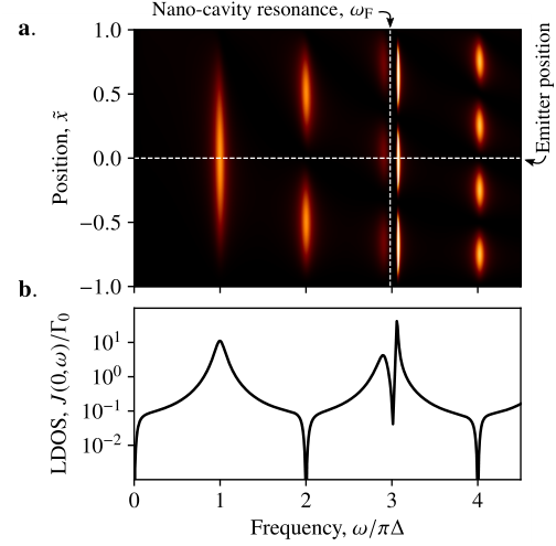
Fig. S2a shows the LDOS of the Fano-cavity, , as a function of position and frequency. Far away from the resonance of the side-coupled cavity (indicated by a dashed vertical line) the partially transmitting element and the left mirror generate simple Fabry-Perot resonances separated by the free spectral range, . Around the resonance of the side-coupled cavity, Fano interference effects give rise to a sharp dip in the LDOS located close to sharp peak. This is more clearly seen in Fig. S2b, where the LDOS for the cavity midpoint () is plotted.
III Mapping
III.1 Effective spectral density of few-mode reservoir
The full Hamiltonian for the solid state emitter and the electromagnetic field is
| (S13) |
where accounts for the free evolution of the emitter as well as the vibrational dynamics of the lattice. The mapped environment consists of two coupled cavity modes, described by bosonic annihilation operators and , both coupled to a common auxiliary bosonic reservoir (labeled by the symbol ) with annihilation operators . The emitter couples to the mapped environment only through the cavity mode (with the real coupling rate ). The full Hamiltonian for this system, , is
| (S14) | ||||
where and are the frequency and overall coupling rate to the mode in the auxiliary reservoir, are unitless complex numbers specifying the relative strength and phase of the mode–reservoir couplings, is a complex coupling rate between the two cavity modes and are their frequencies.
The light-matter coupling terms in both and are of the form , where for we have and for we have . If the initial state of the optical environment is taken as the vacuum, the only non-zero environmental correlation function is , where the expectation value is taken with respect to the free evolution of the environment. Following Ref. Tamascelli et al. 2018, the equivalence between the emitter dynamics generated by and is quantified as the similarity between the two correlation functions
| (S15) | ||||
Equivalently, their corresponding spectral densities, (and similarly for and ) can be used instead. The spectral density of the original system, , can be calculated as the LDOS from Sec. II. For the mapped system, we can calculate using and by tracing out the auxiliary reservoir. Imposing the Markov approximation on the auxiliary reservoir, the master equation corresponding to Eq. (S14) is Breuer and Petruccione 2002
| (S16) | ||||
where and taken frequency-independent, consistent with the Markov approximation.
To calculate the environmental correlation function , we simply set . Since the initial state of the environment is taken as the vacuum state, the system only explores a subspace of the two-cavity Fock space spanned by the basis . In this basis, the Liouvillian corresponding to the RHS of the master equation, Eq. (S16), can be represented by a matrix, which we shall denote by . Since the interaction with the auxiliary environment is taken Markovian, we can calculate using the quantum regression theorem Breuer and Petruccione 2002, allowing for analytic calculation of the corresponding spectral density by matrix exponentiation,
| (S17) | ||||
where in the last equality, we have have defined
| (S18) | ||||
In particular, we see that the spectral density does not depend on all of the complex phases individually, but only on the phase difference . We might thus conveniently set and thus . In this case, the dissipator in the master equation, Eq. (S16), simplifies as .
Analytic structure
The two poles of , denoted by , are found as the roots of the denominator in (S17),
| (S19) | ||||
where and . This allows us to write as
| (S20) |
From this form, we see that are simple poles, and the corresponding residues, , are thus
| (S21) | ||||
III.2 Determining the parameters of the mapped environment

Rather than optimising all of the seven parameters freely using a numerical fitting routine, we exploit our access to analytical properties of and .
By calculating the analytical continuation of in the complex plane in the vicinity of the Fano cavity resonance, two poles can be found (see Fig. S3), which we shall denote by . By numerically integrating along a closed contour, , enclosing a single pole, , the residue of this pole, , can be calculated using the residue theorem as
| (S22) |
Choosing the contour to be a circle with radius , , the residue becomes
| (S23) |
We now require
| (S24) |
Adding these two equations yields
| (S25) | ||||
| (S26) |
Subtracting the two equations (S24) yields . Squaring and taking the real and imaginary parts of this equation leads to
| (S27) | ||||
| (S28) |
Proceeding similarly with the residues and would lead to four additional constraints, which would overdetermine the system. Alternatively, we use the restriction to generate the constraint
| (S29) |
The equations (S25)-(S30) gives five constraints, leaving two degrees of freedom. In our numerical implementation, we leave the two parameters and as free. We then choose the pair that minimises error function , where the integral runs over a frequency window, that covers the central features of the LDOS in the vicinity of the resonance.
IV Polaron master equation and dynamics
IV.1 Master equation
The full Hamiltonian of the mapped optical environment and phonon reservoir is , where is as in Eq. (S14), describes the free evolution of the emitter, describes the free evolution of the phonons and describes the emitter–phonon coupling. In the polaron frame, described by the unitary transformation , with , the Hamiltonian is , where
| (S30) |
describes the internal dynamics of the two-level system and the two mapped optical modes,
| (S31) |
describes the free evolution of the total reservoir comprising the auxiliary electromagnetic environment and the phonon environment, and
| (S32) | ||||
describes the system-reservoir interactions. The quantities entering these expressions are defined as , where is the expectation value of with respect to the phonon thermal state, , with and the Boltzmann constant and temperature, respectively. Tracing out the phonon environment and auxiliary electromagnetic environment leads to the second order Born-Markov master equation for the reduced density operator, Breuer and Petruccione 2002
| (S33) | ||||
where the reference state of the auxiliary electromagnetic environment is taken as the vacuum, , assuming temperatures significantly below the typical optical frequencies around the emitter resonance, . Writing this master equation out explicitly yields
| (S34) |
where the phonon-induced term is
| (S35) |
where , with and denoting the free Heisenberg picture time evolution, . The phonon correlation functions are with and . The phonon spectral density is , with overall coupling strength and cutoff frequency .
IV.2 Dipole spectrum
When calculating dynamics in the polaron frame, quantities of interest must be transformed back to the lab frame. In particular, the dipole correlation function, (with subscript signifying expectation values in the lab frame) is calculated from the polaron frame (subscript ) dynamics as Roy and Hughes 2012
| (S36) |
Assuming that the two-level system and phonons are weakly coupled in the polaron frame, this is approximated as
| (S37) |
and is approximated as the equilibrium phonon correlation function, .
The two-colour emission spectrum, , observed in the waveguide region on the right hand side of the Fano mirror is related to the dipole correlation function as Roy-Choudhury and Hughes 2015; Iles-Smith et al. 2017
| (S38) |
where is the dipole spectrum and
| (S39) |
is the Green’s function that connects the dipole spectrum with the spectrum of the electromagnetic field in the waveguide, transmitted through the Fano mirror Denning et al. 2018.
V Equivalent Fabry-Perot cavity
When both mirrors in the cavity are regular broadband mirrors, a simpler analysis can be carried out. The LDOS in the middle position of the cavity is then
| (S40) |
where is the reflectivity of the right mirror. Following the strategy from Ref. Denning et al. 2018, a single cavity mode can be extracted from the LDOS with reflectivity-dependent emitter coupling strength, , and decay rate, . The master equation describing the dynamics (including interactions with phonons) is then
| (S41) |
where is the annihilation operator of the cavity mode and is as in Eq. (S35), but with . The emission spectrum and indistinguishability is calculated using the same technique as for the Fano cavity, but with the Fabry-Pérot Green’s function
| (S42) |
where is the transmittivity of the right mirror.
Fig. S4 shows the indistinguishability for a Fabry-Pérot cavity as a function of emitter frequency and transmittivity of the right mirror. Besides from the right mirror, all the properties of the optical structure are the same as in Fig. 3 of the main text. The minimal distinguishability of 0.013 is indicated with a dot.
References
- Suh et al. (2004) W. Suh, Z. Wang, and S. Fan, IEEE Journal of Quantum Electronics 40, 1511 (2004).
- Yoon and Magnusson (2013) J. W. Yoon and R. Magnusson, Optics express 21, 17751 (2013).
- Wang et al. (2013) K. X. Wang, Z. Yu, S. Sandhu, and S. Fan, Optics letters 38, 100 (2013).
- Kristensen et al. (2017) P. T. Kristensen, J. R. de Lasson, M. Heuck, N. Gregersen, and J. Mørk, Journal of Lightwave Technology 35, 4247 (2017).
- Yu et al. (2015) Y. Yu, Y. Chen, H. Hu, W. Xue, K. Yvind, and J. Mork, Laser & Photonics Reviews 9, 241 (2015).
- Yu et al. (2017) Y. Yu, W. Xue, E. Semenova, K. Yvind, and J. Mork, Nature Photonics 11, 81 (2017).
- Osterkryger et al. (2016) A. D. Osterkryger, J. R. de Lasson, M. Heuck, Y. Yu, J. Mørk, and N. Gregersen, Optics letters 41, 2065 (2016).
- Gregersen et al. (2016) N. Gregersen, D. P. S. McCutcheon, J. Mørk, J.-M. Gérard, and J. Claudon, Optics express 24, 20904 (2016).
- Denning et al. (2018) E. V. Denning, J. Iles-Smith, A. D. Osterkryger, N. Gregersen, and J. Mork, Physical Review B 98, 121306 (2018).
- Tamascelli et al. (2018) D. Tamascelli, A. Smirne, S. F. Huelga, and M. B. Plenio, Physical Review Letters 120, 030402 (2018).
- Breuer and Petruccione (2002) H.-P. Breuer and F. Petruccione, The theory of open quantum systems (Oxford University Press on Demand, 2002).
- Roy and Hughes (2012) C. Roy and S. Hughes, Physical Review B 85, 115309 (2012).
- Roy-Choudhury and Hughes (2015) K. Roy-Choudhury and S. Hughes, Physical Review B 92, 205406 (2015).
- Iles-Smith et al. (2017) J. Iles-Smith, D. P. S. McCutcheon, A. Nazir, and J. Mørk, Nat. Phot. 11, 521 (2017).