Robust utility maximization under model uncertainty via a penalization approach
This revised version: July 3, 2020
Abstract
This paper addresses the problem of utility maximization under uncertain parameters. In contrast with the classical approach, where the parameters of the model evolve freely within a given range, we constrain them via a penalty function. We show that this robust optimization process can be interpreted as a two-player zero-sum stochastic differential game. We prove that the value function satisfies the Dynamic Programming Principle and that it is the unique viscosity solution of an associated Hamilton–Jacobi–Bellman–Isaacs equation. We test this robust algorithm on real market data. The results show that robust portfolios generally have higher expected utilities and are more stable under strong market downturns. To solve for the value function, we derive an analytical solution in the logarithmic utility case and obtain accurate numerical approximations in the general case by three methods: finite difference method, Monte Carlo simulation, and Generative Adversarial Networks.
Keywords: robust portfolio optimization, differential games, HJBI equation, Monte Carlo, GANs
AMS subject classifications: 49N90, 49K35, 49K20, 49L20, 49L25, 91G80
1 Introduction
This paper addresses the problem of continuous-time utility maximization. Besides the choice of utility function, a key element in the formulation of such a problem is the a priori knowledge assumed for the evolution of the underlying assets (e.g., the expected returns and the quadratic covariation of the diffusion process). In a landmark paper, Merton 1969 found an explicit solution for the problem of optimal portfolio selection and consumption, for a constant relative risk aversion (CRRA) utility function , (a.k.a. power utility or isoelastic utility). He found that the optimal fraction of the wealth to be invested in the risky asset is given by 11 1 Here, is the expected rate of asset returns, is the variance of the asset returns, is the risk-free interest rate and is the relative risk aversion constant., which is independent of both time and the current wealth, even though this quantity is a priori allowed to evolve dynamically. This conclusion is arguably one of the most important results in portfolio optimization (and it is also consistent with the results of Markowitz portfolio optimization Markowitz 1952). It has led to various extensions, some of which are illustrated in the textbook by Rogers 2013.
In the original Merton problem, the evolution of the risky asset, although stochastic by essence, is governed by the Black-Scholes model (Black and Scholes 1973) with fixed parameters and . This is a very simplistic model for the underlying asset price. Stochastic models (for the volatility and interest rates) that describe the price evolution more realistically have later emerged. Several papers have addressed the problem in this context: Matoussi et al. 2015 examined the case of stochastic volatility, while Noh and Kim 2011 addressed the case of stochastic interest rates. The expected return (or drift) plays an essential role in the optimal allocation; even when it is considered stochastic, it is still assumed to be an observable input of the problem. This assumption clearly does not match the reality that investors are facing. Several works by Lakner 1995 and then Bel Hadj Ayed et al. 2017 addressed the utility maximization problem with an uncertain drift, although it was assumed to follow some form of prescribed dynamics or prior distribution.
Two decades ago, the concept of robust portfolio optimization had emerged. It was first introduced in the operations research literature by El Ghaoui and Lebret 1997 and Ben-Tal and Nemirovski 1998. Instead of assuming a model with a known drift, interest rate or volatility, the problem of robust optimal allocation assumes that they will evolve dynamically in the most unfavourable way within a given range. The resulting allocation process tends to be more stable and less vulnerable to changes and misspecifications in model parameters.
There has been a substantial amount of literature on robust portfolio optimization over the last decade and the area is still developing. A comprehensive introduction of the trends and methods can be found in the book by Fabozzi et al. 2007. Gabrel et al. 2014 provided an overview of advances in robust optimization, including but not limited to applications in finance, where they stated that “robustifying” stochastic optimization is one of the key advancements that should develop following the 2007 financial crisis. We list below a few pieces of influential research in this direction. For instance, Elliott and Siu 2009 supposed that an agent wants to maximize the minimal utility function, over a family of probability measures. This problem was then formulated as a Markovian regime-switching model, where the market parameters are modulated by a continuous-time finite-state Markov chain that is determined by the probability measures. Glasserman and Xu 2013 went beyond parameter uncertainties to consider the effect of changes in the probability distributions that define an underlying model. They used relative entropy to quantify the deviation of the worst-case model from a baseline model. Fouque et al. 2016 studied an asset allocation problem with stochastic volatility and uncertain correlation, and derived closed-form solutions for a class of utility functions. Ismail and Pham 2019 studied a robust Markowitz portfolio selection problem under covariance uncertainty. The value function is obtained by optimizing the worst-case mean-variance functional, over the admissible investing strategies . They then solved this problem by the McKean-Vlasov dynamic programming approach and characterized the solution with a Bellman-Isaacs PDE. They also illustrated the robust efficient frontier in two examples: uncertain volatilities and uncertain correlation. Last but not least, we also mention the work by Talay and Zheng 2002, which studied the robust optimization problem in the context of derivatives hedging.
A robust investment process can be interpreted as a two-player game. On one hand, the market can be thought of as an adversarial player controlling the volatility (or the drift) in order to minimize the gains of an investor, on the other hand, the investor, who controls the allocation of the portfolio, is trying to maximize her gains under the worst possible behaviour of the market. The two controllers have conflicting interests, with the gain of one player being a loss for the other. Hence we call this competition between the investor and the market a two-player zero-sum stochastic differential game (SDG). Differential games were first introduced by Isaacs 1965; the book by Fleming and Soner 2006 provides a concise introduction to the theory of viscosity solutions and deterministic zero-sum differential games. The first complete theory for two-player zero-sum SDGs was developed by Fleming and Souganidis 1989, where they proved the existence of value functions of the games. Buckdahn and Li 2008 generalized the results of Fleming and Souganidis 1989 by considering the gain functional as a solution of a Backward Stochastic Differential Equation (BSDE). With the help of BSDE methods, they proved the Dynamic Programming Principle (DPP) for the value functions in a more straightforward approach. Some more recent works on zero-sum SDG include Hernández-Hernández and Sîrbu 2018, Baltas et al. 2019 and Cosso and Pham 2019.
The main novelty of our work is threefold. Firstly, we do not assume a given range of parameters in the evolution of the underlying process. In other papers considering uncertain volatility, the authors assume the admissible , where and are model bounds in accordance with the uncertainty about future fluctuations. Instead, we allow the parameters to move freely and use a penalty function to penalize unrealistic values of the parameters. Mathematically speaking, the penalty function gives some coercivity to the problem so that an optimal solution can be found. This approach has been used for robust derivatives pricing in Tan et al. 2013 and Guo et al. 2017. Note that one can asymptotically recover the aforementioned approaches that involve a fixed parameter range, by taking the penalty function to be 0 over a given set and outside.
Secondly, in the classical papers studying two-player zero-sum SDGs, Fleming and Souganidis 1989 and Nisio 2015 made the assumptions that the domain is bounded and the utility function is bounded and Lipschitz continuous. The present paper extends these results to more general assumptions by considering an unbounded domain and an unbounded utility function . Moreover, we prove that the lower- and upper-value of the SDG (2)-(3) in fact coincide.
Last but not least, we devise two innovative algorithms to compute the value functions, which are control randomization and Generative Adversarial Networks (GANs). In particular, it is, to our knowledge, the first application of the control randomization method (see Kharroubi et al. 2014) in the context of a robust portfolio optimization problem. It is also the first time GANs are used to solve a robust optimization problem in the field of quantitative finance.
GANs are an exciting recent innovation in machine learning. The fundamental principle of GANs is to use two different neural networks as two opponents with conflicting goals, and its solution is a Nash equilibrium. Hence, GANs training is closely related to game theory. Cao et al. 2020 reviewed the minimax structures underlying GANs, and they established theoretical connections between GANs and Mean-Field Games. However, there are few applications of GANs in quantitative finance so far. The only relevant work is by Wiese et al. 2020. Being inspired by GANs’ ability to generate images, they approximated a realistic asset price simulator using adversarial training techniques.
The rest of the paper is organized as follows. In Section 2, we formulate a portfolio optimization problem in a robust setting and introduce the uncertain drift and uncertain volatility processes. In the subsequent sections, we only focus on the uncertain volatility case because the uncertain drift case can be solved in a similar way. In Section 3, we define the value functions for static games and two-player zero-sum SDGs. In Section 4 we show that the differential game has a saddle point and as a consequence, the lower- and upper-values of the SDG coincide. We prove that the value function satisfies the DPP in Section 5 and that our value function is the unique viscosity solution of an HJBI equation in Section 6. In section 7.1, we derive a closed-form solution for the logarithmic utility. In section 7.2, we add some noise to the covariance matrix and simulate portfolios with robust and non-robust strategies, respectively. Then, in section 7.3, we test our robust mechanism by constructing two empirical portfolios using market data. In section 7.4 and 7.5, we provide numerical results for general utility functions using PDE techniques via finite difference methods and Monte Carlo simulations via control randomization. Finally, in section 7.6, we present the algorithm and result of solving a robust portfolio optimization problem with GANs.
2 Problem formulation
We consider a portfolio with risky assets and one risk-free asset compounding at a constant interest rate . The price process of the risky assets is denoted by , and the th element of follows the dynamics
| (1) |
with drift , covariance matrix and its square-root matrix .
We consider a probability space , and processes which are progressively measurable with respect to the -augmented filtration of the -dimensional Brownian motion
Let be the value of the portfolio at time . A portfolio allocation strategy represents the proportion of total wealth the agent invests in the risky assets at time , and is the proportion invested in the risk-free asset.
Assuming the strategy is self-financed, the wealth process evolves as follows
We define with being a -dimensional ones vector. The wealth evolution can be rewritten as
| (2) |
We will follow the framework set in Fleming and Souganidis 1989 and Talay and Zheng 2002. We first introduce the canonical sample spaces for the underlying Brownian motion in (1) and (2). For each , we set
We denote by , the filtration generated by the canonical process from time to time . Equipped with the Wiener measure on , the filtered probability space is the canonical sample space, and is the standard -dimensional Brownian motion.
Now, we introduce the concept of admissible controls.
Definition 1.
An admissible control process (resp. ) for the market on is a progressively measurable process with respect to , taking values in a compact convex set (resp. ), where is a set of symmetric positive semi-definite matrices. The set of all admissible (resp. ) on is compact and convex, denoted by (resp. ).
Definition 2.
An admissible control process for the investor on is a progressively measurable process with respect to , taking values in a compact convex set . The set of all admissible is compact and convex, denoted by .
Note that although the sets for the value of the controls are compact, in practice, where is arbitrarily large.
Next, let us define the payoff function as the expectation of a terminal utility function plus a penalty function :
| (3) |
where denotes the expectation given the initial time and wealth . and is a positive constant. Throughout the paper, we will often include and in the superscript of to indicate the dependency of the wealth process on the allocation, drift and volatility processes. Our objective is to find the optimal portfolio allocation process that maximizes the worst-case payoff function given by the drift process or the covariance process . Throughout the paper, will be a convex function in and .
2.1 Robust value functions
We are now ready to define the value functions. In our problem, the covariance (or drift) is unknown. We want to find the optimal portfolio allocation process that maximizes the worst-case situation given by the covariance (or drift). Then, given an initial condition , this value is given by
We say and are optimal controls if . Hereafter, we focus on the robust optimization problem with an uncertain covariance, that is,
| (4) |
because the uncertain drift case can be studied in a similar manner.
This problem is known as a static game, and the function is called the lower value of the static game. If we reverse the moving order of the two players, we obtain the upper value of the static game, which is
| (5) |
Note that denotes a process controlled by processes . When starts from an initial condition , we write the expectation of as .
2.2 Assumptions
In this section, we make the following assumptions which will hold throughout the paper.
Assumption 1.
The utility function is a continuous, increasing and concave function such that
| (6) |
where is a positive polynomial function.
Assumption 2.
The penalty function is a continuous convex function, and attains its minimum in the interior of .
In addition to Definition 1 and 2, we need the following conditions to ensure the existence and uniqueness of a strong solution of the SDE (2).
Assumption 3.
For any and , we have
and for any fixed value ,
3 Value functions of two-player zero-sum stochastic differential games
In order to complete the description of the game, we need to clarify what information is available to the controllers at each time . For multi-stage discrete time games this can be formulated inductively. However, this is problematic in continuous time, because control choices can be changed instantaneously (Fleming and Soner 2006, Chapter 11). To address this issue, Fleming and Souganidis 1989 adopted the idea of a progressive strategy in a two-player zero-sum SDG, which is defined as follows:
Definition 3.
An admissible strategy (resp. ) for the investor (resp. market) on is a mapping (resp. ) such that, for any and (resp. ), (resp. ) for all implies (resp. ) for all . The set of all admissible strategies for the investor (resp. market) on is denoted by (resp. ).
In the two-player zero-sum SDG, one player is allowed to strategically adapt his control according to the control of his opponent in a non-anticipative fashion. This is in contrast to the static game, in which the player must choose his control without any knowledge of the opponent’s choice. Then, we may define another set of value functions using these admissible strategies: the upper value function of the two-player zero-sum SDG is defined by
| (7) |
and the corresponding lower value function is
| (8) |
The terms “lower” and “upper” are not obvious at first glance, one might first guess the opposite because . We will justify in Corollary 2 using the comparison principle.
4 Existence of a value for the differential games
In this section, we prove that the four value functions defined in the previous sections all coincide, i.e., . This is established via the following propositions.
Proposition 1.
Proof.
The inequality holds because contains constant mappings, i.e., for any and fixed . Similarly, holds because contains a copy of . Then for all and , there exists some such that
So . A similar argument gives us . Hence we have
In order to complete the proof, it suffices to show that . This is proven in Corollary 2. ∎
Proposition 2.
Let be a continuous, increasing and concave utility function on , suppose that Assumption 2 holds, then .
Proof.
See Appendix A.1. ∎
Using Proposition 2, we can conclude that there exists a value for the two-player zero-sum SDG, i.e., . We focus on the analysis of in the following sections.
5 Dynamic programming principle
If the drift and volatility functions of dynamics (2) and the utility function were bounded and was Lipschitz continuous, we could apply the results of Fleming and Souganidis 1989 directly. However, in our model, the drift and volatility functions are unbounded and is only locally Lipschitz continuous. So we must extend the classical results and use localization techniques to prove that the value function defined in (7) satisfies the Dynamic Programming Principle (DPP). The DPP is widely used in numerical methods, such as the least squares Monte Carlo method.
Before presenting the main result, we require the following important property of the value function.
Proposition 3.
Proof.
See Appendix A.2. ∎
We are now in the position to present a main result in this paper.
Theorem 1 (Dynamic Programming Principle).
Proof.
See Appendix A.3. ∎
As a consequence of the DPP, the value function satisfies the following property.
Corollary 1.
Proof.
See Appendix A.4. ∎
6 Viscosity solution of the HJBI equation
In this section, we prove that the value function is the unique viscosity solution of a Hamilton-Jacobi-Bellman-Isaacs equation. In 6.1, we prove the existence of the viscosity solution, and we state the uniqueness of this viscosity solution in 6.2.
6.1 Existence of a viscosity solution of the HJBI Equation
Now we state another main result in this paper; the proof is a modification of Talay and Zheng 2002.
Theorem 2.
Suppose that Assumptions 1, 2 and 3 hold true. Then the value function defined in (7) is a viscosity solution of the HJBI equation
| (12) |
where
| (13) |
for .
Proof.
See Appendix A.5. ∎
6.2 Comparison principle for the HJBI Equation
In this subsection, we present the comparison principle for equation (12), which implies the uniqueness of the viscosity solution of the HJBI equation. We can adapt the proof from Pham 2009 for an HJB equation and straightforwardly extend it to HJBI equations with two controls.
Theorem 3.
Comparison Principle (Pham 2009).
As a consequence of the comparison principle, the function (7) is in fact the unique viscosity solution of the HJBI equation (12).
Corollary 2.
Proof.
From Theorem 2, is a viscosity solution of the HJBI equation (12). Let be a test function such that is a local minimum of . Using the viscosity supersolution property of , we have
where is defined by (13). Define
| (15) |
It is obvious that , so
Thus is a supersolution of the HJBI equation
Using the results of Fleming and Souganidis 1989 and a similar argument, we can prove the lower value function (8) is the unique viscosity solution of the HJBI equation
| (16) |
Finally, by the comparison principle, we have , as required. ∎
7 Numerical results
In this section, we provide a few numerical examples with commonly used utility functions. We first establish an analytical solution in the case of the Logarithmic utility function. Then we numerically approximate the value functions for both the Logarithmic and CRRA utility functions using an implicit finite difference method, a control randomization method, and a Generative Adversarial Network method.
7.1 Analytical solution
In the first example, we consider and the penalty function . It is possible to find the explicit solution for the value function as well as the optimal controls. Writing explicitly, the value function becomes:
| (17) | ||||
To find the optimal and , we can differentiate instantaneously the integrand with respect to and respectively. Then we obtain the following optimality conditions:
| (18) | ||||
| (19) |
which leads to a quartic equation
| (20) |
The optimal and can be solved from equation (20) explicitly; we provide the solution in the Appendix A.6. The equation (20) always has a real positive root, hence the optimal volatility and optimal strategy . By substituting the optimal controls into (17), we obtain the analytical solution of the value function. From equations (18)–(19), we observe that the optimal volatility and investment strategy are both constants, being independent of the wealth and the time . The classical optimal portfolio strategy given by Merton is also a constant, where for CRRA utility functions. However, in our problem, it is not possible to find an analytical solution for a power utility function. We will use numerical methods to estimate the values in the next subsection. It is worth mentioning that, when , we can apply the above method to portfolios with multiple risky assets and get the analytical solutions by solving a system of optimality conditions. The detailed process is very similar, hence omitted here. Moreover, the reference volatility is not necessarily a constant, it can be a local volatility depending on time and stock price. However, for multiple assets, it would increase the dimension of the problem.
7.2 Comparison of robust and non-robust portfolios with Monte Carlo simulation
In this section, we implement our robust strategy using Monte Carlo simulations, and compare the performance of robust and non-robust portfolios.
As we know, in the real world volatility estimates are noisy and biased, though likely to oscillate around a reference value in the long run. In the first experiment, we have a reference covariance matrix , which is estimated according to historical data. We assume that the real-world covariance is the reference covariance plus some noise. We construct robust and non-robust portfolios consisting of two risky assets and one risk-free asset. For the robust portfolio, we use ( denotes the usual Frobenius norm) as the penalty function, then the analytical robust investment strategy can be calculated in a similar method to the one in section 7.1. For the non-robust one, we use as the covariance, then calculate the non-robust strategy accordingly. Assuming the real covariance matrix during the investment process is , where the noise follows a standard normal distribution and is the magnitude of the noise, we use Monte Carlo simulations to estimate the expected utility function
| (21) |
We substitute in (21) for the robust portfolio, and for the non-robust one.
The results with various are shown in Figures 7.2 to 7.2, where we used paths in the simulation and the initial wealth . We can observe that the robust portfolio may underperform when there is little noise. But, as the noise size increases, the robust strategy will outperform the non-robust strategy eventually. Comparing Figures 7.2, 7.2 and 7.2, we can find that when the penalty is relatively weak (), it takes a bigger noise size for the robust strategy to outperform. When the penalty is stiff (), the robust strategy will outperform with a very small noise size. The robust expected utility is almost a constant for all sizes of noise in Figure 7.2, meaning that our model is very robust to changes in market circumstances. Among the three values of illustrated, Figure 7.2 is probably the most attractive to investors. When the reference is perfect, the robust portfolio only loses to the non-robust one by a little, but when is wrong, the robust portfolio outperforms the non-robust one by a large amount. It means the price we pay for the robustness is tolerable, but the potential reward is substantial.
Define the crossing point as the value of for which the robust expected utility matches the non-robust expected utility. Figure 7.2 depicts how the crossing point varies with respect to . It tells us how much should our reference covariance be wrong for the robust portfolio to outperform the non-robust portfolio. The behaviour of the robust portfolio varies with . For a certain , by looping over a range of , we can find the one giving us the maximal robust expected utility. This relation is plotted in Figure 7.2. With this plot, if we know how confident we are with the reference (i.e., the value of ), we can choose the best for robust portfolio allocation.
![[Uncaptioned image]](1907.13345v5/robust_simulation_2asset_la001.png) \captionof
\captionof
figureExpected utility with
![[Uncaptioned image]](1907.13345v5/robust_simulation_2asset_la1.png) \captionof
\captionof
figureExpected utility with
![[Uncaptioned image]](1907.13345v5/robust_simulation_2asset_la70.png) \captionof
\captionof
figureExpected utility with
![[Uncaptioned image]](1907.13345v5/epsilon_vs_lambda_2asset.png) \captionof
\captionof
figure
![[Uncaptioned image]](1907.13345v5/la_best_log10.png) \captionof
\captionof
figure
7.3 Comparison of robust and non-robust portfolios with empirical market data
In the second experiment, we implement the robust and non-robust strategies with empirical market data. We have portfolios, and we construct each portfolio according to robust and non-robust allocations, respectively. Each portfolio consists of risky assets and risk-free asset, with a maturity of year. The portfolios’ starting dates range from 02/04/15 to 03/04/19 (for example, the st portfolio starts on 02/04/15 and lasts for one year, the th portfolio starts on 03/04/19 and lasts for one year as well). We choose the SP500 (GSPC) and SPDR Gold Shares (GLD)22 2 Stock prices are downloaded from Yahoo Finance. as our risky assets and use a constant interest rate . For a specific portfolio, we set to be the sample covariance estimator of the years of daily relative returns before the starting date. The estimated annual expected returns are the exponentially weighted moving average of the daily relative returns with a -year lookback window and -year half-life. With a decay parameter , for the th portfolio, .
In this experiment, we use a logarithmic utility function and a penalty function . At the beginning of the investment process for each portfolio, we estimate parameters and then compute the robust and non-robust portfolio allocations accordingly. Starting from an initial wealth , the wealth of the non-robust portfolio evolves as
| (22) |
where are the non-robust allocations on day . For the wealth of the robust portfolio, just replace with the robust allocations in (22). Finally, by averaging the of all the portfolios, we get the expected utility function.
Figures 7.3–7.3 present the terminal wealth of the robust and non-robust portfolios. For a small , the robust portfolios are very stable. No matter how the market changes, the robust terminal wealth stays around . As increases, the robust portfolios start to show fluctuations. Eventually, their behaviour converges to that of the non-robust portfolios as approaches to infinity, which corresponds to the non robust case. This behaviour is consistent with our expectations. The penalty function is not playing its role when is close to zero. Hence the robust allocations are optimal for the most chaotic market situations, and the investment strategies are very conservative. As becomes larger, the penalty function comes into play and prevents extreme volatilities. As a consequence, the robust strategies are less conservative, and portfolios will show more fluctuations under regime changes.
We show the robust and non-robust expected utilities in Figure 1. It depicts how and change w.r.t. . We can compare this plot with Figures 7.2, 7.2, 7.2 and 7.2 in section 7.2. For a given amount of noise, the robust portfolio may underperform for small , but the value will increase gradually and reach a highest point. Finally, the robust expected utility will converge to the non-robust one.
![[Uncaptioned image]](1907.13345v5/new_la001.png) \captionof
\captionof
figureTerminal wealth with
![[Uncaptioned image]](1907.13345v5/new_la10.png) \captionof
\captionof
figureTerminal wealth with
![[Uncaptioned image]](1907.13345v5/new_la100.png) \captionof
\captionof
figureTerminal wealth with
![[Uncaptioned image]](1907.13345v5/new_la1000.png) \captionof
\captionof
figureTerminal wealth with

To illustrate the time evolution of the portfolio wealth, we show the stock prices and wealth of two portfolios, starting on 2017-01-03 (Figure 2) and 2018-01-26 (Figure 3), respectively. For the portfolio in Figure 2, the optimal non-robust allocations are , and the robust allocations with are . The allocations are both constant, independent of time. The SP500 keeps rising in Figure 2a, while there are some fluctuations in the Gold price. Over the same period, the absolute performance of the non-robust portfolio is better all the way (Figure 2b). For the portfolio in Figure 3, we have , and . Since the proportions invested in Gold are small for both robust and non-robust portfolios, the trend of wealth is dominated by the price of SP500. There are two big drops happening in Feb. 2018 and Dec. 2018, respectively. These are also reflected in the portfolio wealth in Figure 3b. However, compared with the non-robust strategy, the robust strategy is more conservative. Hence, the robust portfolio loses less during the market shocks and outperforms the non-robust one.


From the above empirical experiments and the Monte Carlo simulations from subsection 7.2 , we can see that, by adding this robust mechanism with a properly chosen , the portfolio value can overcome a wrong covariance matrix estimate and is less vulnerable to sudden market shocks. Furthermore, unlike other robust methods which only consider the worst case, our model is more flexible and provides a greater range of more practical in-between option.
7.4 Implicit finite difference method
In this section, we are computing the value function via an implicit finite difference method. We use the penalty function for simplicity. Then the HJBI equation is
| (23) |
where the Hamiltonian is defined by
| (24) |
Solving for the optimal controls in (24) using the first order condition, we obtain and . Substituting and into the PDE (23), we obtain
where . Note we have shown in Section 4 that .
Since the PDE (23) is non-linear, in order to use the implicit finite difference method, we first linearize the function with respect to the second order term via the Legendre transform. This method was also used by Jonsson and Sircar 2002a; Jonsson and Sircar 2002b to solve nonlinear HJB equations. We also combine the linearization step with a fixed-point iteration scheme.
Define as the Legendre transform of with respect to the second order term; it is given by
where . Hence, we can represent as the supremum of linear functions of ,
| (25) |
It is difficult to check the condition for stability in our PDE as the optimal is unknown. Fortunately, implicit finite difference methods have a weaker requirement for stability than explicit finite difference methods.
We set the time grid as , and the spatial grid as . With the maturity , we use a constant time step and a constant spatial step . We apply a forward approximation for , a central approximation for , and a standard approximation for . Working backward in the implicit scheme, at each time step , the optimal in (25) is the solution of the first order condition or equivalently,
| (26) |
Although we do not have the true values for as the values of depend on , we can use a fixed-point iteration scheme to find the solution of equation (26). First we make an initial guess using the known values , then iteratively generate a sequence with until converges.
Finally we can substitute the discrete approximations of the derivatives into the HJBI equation (23), and we obtain the implicit form:
| (27) |
Let be the coefficient matrix, the value vector at time and the right hand side of (27). Then equation (27) can be written in a matrix notation:
The algorithm for this method is summarized in Algorithm 1.
for step do
- 1.
Solve using , and get the value vector
- 2.
Solve using , where the values are from . Then get the value vector .
- 3.
Repeat step 2 until
- 4.
Let
7.4.1 Logarithmic utility function
In the 1-asset example, we use the logarithmic utility function and the penalty function . The terminal condition is given by the utility function,
The boundary conditions and for are given explicitly by the equation
with
![[Uncaptioned image]](1907.13345v5/Im_fin_diff.png) \captionof
\captionof
figure,
![[Uncaptioned image]](1907.13345v5/fin_diff_true_2d.png) \captionof
\captionof
figure,
Similarly, we can also implement the above method on a 2-asset example where and . The HJBI equation becomes
| (28) |
We can solve for the optimal controls in (28) using the first order condition. In this example, we always have the optimal and . Then, by applying Algorithm 1, we can get the value function of a portfolio with 2 risky assets.
Figure 7.4.1 shows the PDE estimated for the 1-asset example with parameters ; Figure 7.4.1 shows result for the 2-asset case with parameters . Comparing with the analytical solution, we can see that the two curves completely overlap for both 1-asset and 2-asset cases, which validates the accuracy of the PDE approach.
7.4.2 Power utility function
In the second example, we use a power utility function. This time, we only have the terminal condition and the boundary condition for , but not the boundary condition for a large . For functions where , the limit of the first order derivative approaches as goes to infinity. Therefore we can use a zero Neumann boundary condition when is large. Then we have the following terminal and boundary conditions:
Figure 4a shows the simulated value for a range of , with and parameters . We only display the estimated curve computed by our PDE method, as there is no analytical solution available for comparison in this example. Figure 4b shows the first four iterations of the estimated from an initial guess. There is almost no difference between the four curves, indicating that the fixed point iteration scheme has converged within the first four iterations.


This subsection has shown that the PDE method converges to the true value efficiently. Nevertheless, there are a few shortcomings to this approach:
- •
The PDE approach requires tedious algebraic manipulation before implementation. In particular, even when using the same utility function, the preliminary computations have to be redone if we switch to a different penalty function.
- •
In general, PDE approaches suffer from the curse of dimensionality. As the dimension of the problem becomes higher, the computational complexity increases exponentially and the approach becomes infeasible. Although the PDE approach suffices for our current problem as the wealth process is only one-dimensional, it may not be feasible for other problems arising from multidimensional stochastic differential games.
For these two reasons, in the next subsection we develop a numerical scheme based on Monte Carlo simulations, which can be potentially useful for high-dimensional problems or in the case of complex penalty functions.
7.5 Monte Carlo method
In this section, we implement a Regression Monte Carlo scheme to solve the same robust portfolio allocation problems. Carriere 1996 introduced the Regression Monte Carlo approach to solve optimal stopping problems for any Markovian process in discrete time. In particular, he used non-parametric regression techniques. Later, Tsitsiklis and Van Roy 2001 and Longstaff and Schwartz 2001 used a similar scheme with ordinary least squares (a.k.a. Least Squares Monte Carlo) to value American options, respectively by value iteration and by performance iteration (see for example Denault and Simonato 2017). Since then, Regression Monte Carlo has become a popular tool in option pricing and more generally for solving discrete-time stochastic control problems in finite horizon.
First of all, we discretize the time interval into time steps with a constant step size . Using the Euler scheme on the logarithm of the state variable, one obtains the following dynamics for the discrete-time wealth :
| (29) |
and the discretized form of our value is
| (30) |
As we have proved in Section 5, this value function satisfies the DPP:
| (31) |
7.5.1 Control randomization
Inspired by the Dynamic Programming Principle, we can start from the known terminal condition and compute the value functions backward in time recursively. Equation (31) involves a conditional expectation, which cannot be computed explicitly. Instead, one can for example use a least squares regression to approximate with a polynomial basis function. The obstacle in the implementation is that we are not able to simulate the paths forward, since the dynamics of the state variable depends on the uncertain controls. Following Kharroubi et al. 2014, one way to tackle this problem is an initial randomization of the controls, i.e., we choose an arbitrary initial distribution for the controls and simulate the with these dummy and , before including these dummy controls in the regressors of the least-squares regressions.
Proofs of the convergence and error bounds for standard Regression Monte Carlo are available in Clément et al. 2002 and Beutner et al. 2013 for example. In the case of controlled dynamics, Kharroubi et al. 2015 analyzed the time-discretization error, and Kharroubi et al. 2014 investigated the projection error generated by approximating the conditional expectation by basis functions for the control randomization scheme. Recently, alternative randomization schemes have been proposed in the literature, such as Ludkovski and Maheshwari 2019, Balata and Palczewski 2018, Bachouch et al. 2018 or Shen and Weng 2019, which are more amenable to comprehensive convergence proofs, see Balata and Palczewski 2017 and Huré et al. 2018. Nevertheless, the classical control randomization scheme retains some advantages, such as the ease with which it can handle switching costs, as shown in Zhang et al. 2019.
For the choice of basis function , we can use a polynomial function in , and let . Once we complete the regression, we can approximate the conditional expected value function in (31) by . For the th simulation path, we can find the optimal controls by:
The complete process is shown in Algorithm 2.
Backward Regression:
- 1.
Choose an initial distribution and generate initial random controls accordingly.
- 2.
Generate paths of state variable . The th path starts from the initial condition , evolves following the dynamics with and assign .
- 3.
For do
- (a)
Regress on , and get the regression coefficients
- (b)
Find the optimal controls by
- (c)
The value function at time step is
- (a)
- 4.
The value function
Forward Resimulation:
- 1.
Set the initial condition
- 2.
For
- (a)
Find the optimal controls by , using the regression coefficients obtained in the backward part and the new state variable .
- (b)
The state variable at time step is
- (a)
- 3.
The forward simulated value function
7.5.2 Logarithmic utility function
We first consider an example with 1 risky asset. When the utility function is logarithmic and the penalty function is , we choose the following basis function
To find the optimal controls, we differentiate with respect to and , then we can get the optimal controls by solving the following polynomial equation
With , there exists a real positive root. We can see the optimal controls are constants for each step, being independent of the state variable , this is the same as our observation in the analytical solution.
We used paths, and step size in the simulation, with the parameters . Figure 6 shows the backward regression values, forward resimulation values and true values as we change the parameter . Figure 6 compares the forward resimulation values, finite difference results and true values as we change the parameter . It shows that both the PDE and Monte Carlo approach the true value in this example.


For the example with risky assets, we use the logarithmic utility function and the penalty function . We choose the following basis function in this case:
where are the volatilities of the two assets and is the correlation between the assets. We can differentiate to get the optimal controls. In practice, we always have , but we need to truncate to . The optimal controls are also constants for each step as in the 1-asset case.
In the implementation, we use paths, and step size . The result is provided in Figure 8. This plot compares the backward regression values, forward resimulation values and the analytical values, and it shows how the values change w.r.t. the penalty strength . From our observation, the average of the forward and backward results yields an even better estimate.
We can observe from Figure 6 and 8 that, as claimed in Kharroubi et al. 2014, the value function estimated at the end of the backward loop serves as an upper bound for the true value, while the one obtained from the forward resimulation serves as a lower bound and has a smaller error than the upper bound.
7.5.3 Power utility function
Here we show a 1-asset example with power utility. When the utility function is and the penalty function , we choose the basis function
| (32) |
To find the optimal controls, we differentiate and then get the polynomial equation (33) for each path. We can see the optimal controls and depend on in this case.
| (33) |
Figure (8) shows Monte Carlo and finite difference approximations for a range of drifts , with , , . We can see that the PDE estimates lie within the Monte Carlo bounds and that the forward simulation values almost overlap the PDE estimations. Although we do not have the analytical solution for this power utility case, these plots suggest that we are able to estimate the true values accurately with both Control Randomization and Finite Difference.
In both the logarithmic and power utility cases, the forward resimulation always performs better than the backward loop estimates. That is because the forward resimulation only suffers from one source of error, the optimal control estimation, while the backward regression suffers more directly from regression error (see Kharroubi et al. 2014). So the forward simulation result is a better estimator of the true value and is the one we use for comparison with the analytical and PDE approaches.
From the results above, we can see that for these robust portfolio allocation problems with one single risky asset, both PDE and Monte Carlo methods provide accurate estimates, with the PDE estimates being slightly better overall. Both methods can be considered for solving robust portfolio allocation problems in practice. Some difficulties with the Monte Carlo approach are the choice of the basis and the number of Monte Carlo paths needed for a stable convergence. Still, the Monte Carlo would be the method of choice for more realistic portfolio allocation with multiple risky assets (see Zhang et al. 2019), as the PDE approach could quickly become computationally intractable in this situation.
7.6 Generative Adversarial Networks
In this section, we devise a GAN-based algorithm to solve the two-player zero-sum differential game.
Generative Adversarial Networks were introduced in Goodfellow et al. 2014. A GAN is a combination of two competing (deep) neural networks: a generator and a discriminator. The generator network tries to generate data that looks similar to the training data, and the discriminator network tries to tell the real data from the fake data. The idea behind GANs is very similar to the robust optimization problem studied in our paper: GANs can be interpreted as minimax games between the generator and the discriminator, whereas our problem is a minimax game between the agent who controls the portfolio allocation and the market who controls the covariance matrix. Inspired by this connection, we propose the following GAN-based algorithm.
Our GANs are composed of two neural networks; one generates (-generator), the other generates (-generator). The two networks have conflicting goals, the -generator tries to maximize the expected utility, while the -generator wants to minimize the expected utility. They compete against each other during the training. Because we have two networks with different objectives, it cannot be trained as a regular neural network. Each training iteration is divided into two phases: In the first phase, we train the -generator, with the loss function . Then the back-propagation only optimizes the weights of the -generator. In the second phase, given the output from the -generator, we train the -generator with a loss function . During this phase, the weights of the -generator are frozen and the back-propagation only updates the weights of the -generator. In a zero-sum game, the -generator and -generator constantly try to outsmart each other. As training advances, the game may end up at a Nash Equilibrium.
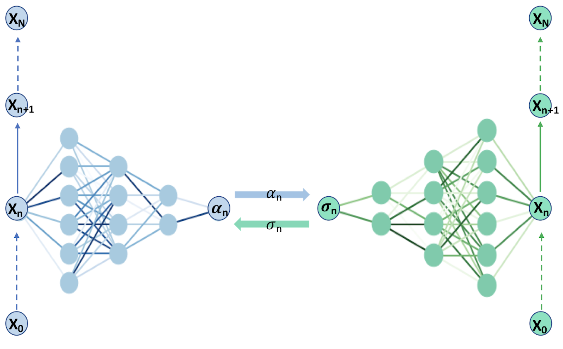
A demonstration of the simplified network architecture is illustrated in Figure 9. The blue part on the left of Figure 9 is the -generator. For each time step , we construct a network (), with the input and parameter , the network generates output . With the dynamics of wealth (29), we can continue this process until we get the terminal wealth . Once we get the output , we can use them as parameters for the -generator (the green part in the figure). In the -generator, similarly, we have one network () for each time step . With the input and parameter , we can generate . At the end of this phrase, the sequence will be fed into the -generator as parameters as well. We have summarized this training process for 1-asset examples in Algorithm 3.
In the implementation, we choose the parameters . The training data has a sample size . We discretize the investment process into time steps. The deep neural network for each time step contains hidden layers, using Leaky ReLU as the activation function. For the generator, to ensure the positivity of the output, we use Leaky Sigmoid as the activation function of the output layer. It is defined as . Its shape is similar to Sigmoid, but its range is . We train the first epochs with a learning rate , and then we train another epochs with a decreased learning rate .
Given the initial condition , and the initial starting point of :
for epoch do
We now assess the quality of Algorithm 3. Firstly, we use a utility function and a cost function . Assuming the portfolio has an initial wealth , the analytical solution facilitates numerical comparison. Figures 10a compares the learned value functions with the true values for a range of . It shows good accuracy of the learned functions versus the true ones. The errors are of magnitude . The loss function during the training is presented in Figure 10b. Unlike the trend in training regular deep neural networks, the loss function is not monotonically decreasing. As we can see, the minimizer was dominating the competition at the beginning, the loss function decreasing rapidly. Then the maximizer caught up, the loss function increased for a while and finally converged to the true value.
In the second example, we use a utility function and a cost function . We set in this case and estimate the value functions for a range of . Since we do not have access to the true values for power utility, we compare the GANs estimated values with the PDE estimations in 11a. The loss function for during the training is presented in Figure 11b.


Despite the promising results, a limitation of GANs, shared with deep neural networks in general, is the sensitivity of training to the chosen parameters. On difficult problems, fine-tuning the hyper-parameters of the GAN to facilitate training might require a lot of effort. One standard strategy for stabilizing training is to carefully design the model, either by adopting a proper architecture (Radford et al. 2015) or by selecting an easy-to-optimize objective function (Salimans et al. 2016). In spite of this caveat, GANs can be considered a viable contender to the more classical Monte Carlo methods of subsection 7.5 for robust portfolio allocation involving multiple risky assets, and deserve further investigation.
8 Conclusion
In this paper, we interpreted a robust portfolio optimization problem as a two-player zero-sum stochastic differential game. We have proven that the value function is the unique viscosity solution of a Hamilton–Jacobi–Bellman–Isaacs equation, and satisfies the Dynamic Programming Principle. We compared the performance of the robust and non-robust portfolios with both Monte Carlo simulation and empirical market data. Under market shocks, our robust mechanism can prevent huge losses. By choose the properly, the robust portfolios have a higher expected utility than the non-robust one. In addition to the finite difference method, we provide control randomization and GANs algorithms to estimate the value function. These two methods can enrich quantitative techniques for solving robust portfolio optimization problems. Both of them have demonstrated high accuracy in the numerical results.
Acknowledgements
The Centre for Quantitative Finance and Investment Strategies has been supported by BNP Paribas. Ivan Guo has been partially supported by the Australian Research Council Discovery Project DP170101227.
References
- Bachouch et al. (2018) Bachouch, A., C. Huré, N. Langrené, and H. Pham (2018). Deep neural networks algorithms for stochastic control problems on finite horizon: numerical applications. arXiv preprint arXiv:1812.05916.
- Balata and Palczewski (2017) Balata, A. and J. Palczewski (2017). Regress-later Monte Carlo for optimal control of Markov processes. arXiv preprint arXiv:1712.09705.
- Balata and Palczewski (2018) Balata, A. and J. Palczewski (2018). Regress-later Monte Carlo for optimal inventory control with applications in energy. arXiv preprint arXiv:1703.06461.
- Baltas et al. (2019) Baltas, I., A. Xepapadeas, and A. N. Yannacopoulos (2019). Robust control of parabolic stochastic partial differential equations under model uncertainty. European Journal of Control 46, 1–13.
- Bel Hadj Ayed et al. (2017) Bel Hadj Ayed, A., G. Loeper, and F. Abergel (2017). Forecasting trends with asset prices. Quantitative Finance 17(3), 369–382.
- Ben-Tal and Nemirovski (1998) Ben-Tal, A. and A. Nemirovski (1998). Robust convex optimization. Mathematics of operations research 23(4), 769–805.
- Beutner et al. (2013) Beutner, E., A. Pelsser, and J. Schweizer (2013). Fast convergence of regress-later estimates in least squares Monte Carlo.
- Black and Scholes (1973) Black, F. and M. Scholes (1973). The pricing of options and corporate liabilities. Journal of Political Economy 81(3), 637–654.
- Buckdahn and Li (2008) Buckdahn, R. and J. Li (2008). Stochastic differential games and viscosity solutions of Hamilton–Jacobi–Bellman–Isaacs equations. SIAM Journal on Control and Optimization 47(1), 444–475.
- Cao et al. (2020) Cao, H., X. Guo, and M. Lauriere (2020). Connecting GANs and MFGs. arXiv preprint arXiv:2002.04112.
- Carriere (1996) Carriere, J. F. (1996). Valuation of the early-exercise price for options using simulations and nonparametric regression. Insurance: Mathematics and Economics 19(1), 19–30.
- Clément et al. (2002) Clément, E., D. Lamberton, and P. Protter (2002). An analysis of a least squares regression method for American option pricing. Finance and Stochastics 6(4), 449–471.
- Cosso and Pham (2019) Cosso, A. and H. Pham (2019). Zero-sum stochastic differential games of generalized McKean–Vlasov type. Journal de Mathématiques Pures et Appliquées 129, 180–212.
- Denault and Simonato (2017) Denault, M. and J.-G. Simonato (2017). Dynamic portfolio choices by simulation-and-regression: revisiting the issue of value function vs portfolio weight recursions. Computers & Operations Research 79, 174–189.
- El Ghaoui and Lebret (1997) El Ghaoui, L. and H. Lebret (1997). Robust solutions to least-squares problems with uncertain data. SIAM Journal on matrix analysis and applications 18(4), 1035–1064.
- Elliott and Siu (2009) Elliott, R. J. and T. K. Siu (2009). Robust optimal portfolio choice under Markovian regime-switching model. Methodology and Computing in Applied Probability 11(2), 145–157.
- Fabozzi et al. (2007) Fabozzi, F. J., P. N. Kolm, D. A. Pachamanova, and S. M. Focardi (2007). Robust portfolio optimization and management. John Wiley & Sons.
- Fleming and Soner (2006) Fleming, W. H. and H. M. Soner (2006). Controlled Markov processes and viscosity solutions, Volume 25. Springer Science & Business Media.
- Fleming and Souganidis (1989) Fleming, W. H. and P. E. Souganidis (1989). On the existence of value functions of two-player, zero-sum stochastic differential games. Indiana University Mathematics Journal 38(2), 293–314.
- Fouque et al. (2016) Fouque, J.-P., C. S. Pun, and H. Y. Wong (2016). Portfolio optimization with ambiguous correlation and stochastic volatilities. SIAM Journal on Control and Optimization 54(5), 2309–2338.
- Gabrel et al. (2014) Gabrel, V., C. Murat, and A. Thiele (2014). Recent advances in robust optimization: An overview. European Journal of Operational Research 235(3), 471–483.
- Glasserman and Xu (2013) Glasserman, P. and X. Xu (2013). Robust portfolio control with stochastic factor dynamics. Operations Research 61(4), 874–893.
- Goodfellow et al. (2014) Goodfellow, I., J. Pouget-Abadie, M. Mirza, B. Xu, D. Warde-Farley, S. Ozair, A. Courville, and Y. Bengio (2014). Generative adversarial nets. In Advances in neural information processing systems, pp. 2672–2680.
- Guo et al. (2017) Guo, I., G. Loeper, and S. Wang (2017). Local volatility calibration by optimal transport. arXiv preprint arXiv:1709.08075.
- Hernández-Hernández and Sîrbu (2018) Hernández-Hernández, D. and M. Sîrbu (2018). Zero-sum stochastic differential games without the Isaacs condition: random rules of priority and intermediate Hamiltonians. SIAM Journal on Control and Optimization 56(3), 2095–2119.
- Huré et al. (2018) Huré, C., H. Pham, A. Bachouch, and N. Langrené (2018). Deep neural networks algorithms for stochastic control problems on finite horizon: convergence analysis. arXiv preprint arXiv:1812.04300.
- Isaacs (1965) Isaacs, R. (1965). Differential games: a mathematical theory with applications to warfare and pursuit, control and optimization. SIAM Series in Applied Mathematics. Wiley, New York.
- Ismail and Pham (2019) Ismail, A. and H. Pham (2019). Robust Markowitz mean-variance portfolio selection under ambiguous covariance matrix. Mathematical Finance 29(1), 174–207.
- Jonsson and Sircar (2002a) Jonsson, M. and K. R. Sircar (2002a). Partial hedging in a stochastic volatility environment. Mathematical Finance 12(4), 375–409.
- Jonsson and Sircar (2002b) Jonsson, M. and R. Sircar (2002b). Optimal investment problems and volatility homogenization approximations. In Modern Methods in Scientific Computing and Applications, pp. 255–281. Springer.
- Kharroubi et al. (2014) Kharroubi, I., N. Langrené, and H. Pham (2014). A numerical algorithm for fully nonlinear HJB equations: an approach by control randomization. Monte Carlo Methods and Applications 20(2), 145–165.
- Kharroubi et al. (2015) Kharroubi, I., N. Langrené, and H. Pham (2015). Discrete time approximation of fully nonlinear HJB equations via BSDEs with nonpositive jumps. Annals of Applied Probability 25(4), 2301–2338.
- Lakner (1995) Lakner, P. (1995). Utility maximization with partial information. Stochastic Processes and their Applications 56(2), 247–273.
- Longstaff and Schwartz (2001) Longstaff, F. A. and E. S. Schwartz (2001). Valuing American options by simulation: a simple least-squares approach. The Review of Financial Studies 14(1), 113–147.
- Ludkovski and Maheshwari (2019) Ludkovski, M. and A. Maheshwari (2019). Simulation methods for stochastic storage problems: A statistical learning perspective. Energy Systems, 1–39.
- Markowitz (1952) Markowitz, H. M. (1952). Portfolio selection/Harry Markowitz. The Journal of Finance 7(1), 77–91.
- Matoussi et al. (2015) Matoussi, A., D. Possamaï, and C. Zhou (2015). Robust utility maximization in nondominated models with 2BSDE: the uncertain volatility model. Mathematical Finance 25(2), 258–287.
- Merton (1969) Merton, R. C. (1969). Lifetime portfolio selection under uncertainty: The continuous-time case. The Review of Economics and Statistics, 247–257.
- Nisio (2015) Nisio, M. (2015). Stochastic control theory, Volume 72. Springer Science & Business Media.
- Noh and Kim (2011) Noh, E.-J. and J.-H. Kim (2011). An optimal portfolio model with stochastic volatility and stochastic interest rate. Journal of Mathematical Analysis and Applications 375(2), 510–522.
- Pham (2009) Pham, H. (2009). Continuous-time stochastic control and optimization with financial applications, Volume 61. Springer Science & Business Media.
- Radford et al. (2015) Radford, A., L. Metz, and S. Chintala (2015). Unsupervised representation learning with deep convolutional generative adversarial networks. arXiv:1511.06434.
- Rogers (2013) Rogers, L. C. (2013). Optimal investment. Springer.
- Salimans et al. (2016) Salimans, T., I. Goodfellow, W. Zaremba, V. Cheung, A. Radford, and X. Chen (2016). Improved techniques for training GANs. In Advances in neural information processing systems, pp. 2234–2242.
- Shen and Weng (2019) Shen, Z. and C. Weng (2019). A backward simulation method for stochastic optimal control problems. arXiv preprint arXiv:1901.06715.
- Talay and Zheng (2002) Talay, D. and Z. Zheng (2002). Worst case model risk management. Finance and Stochastics 6(4), 517–537.
- Tan et al. (2013) Tan, X., N. Touzi, et al. (2013). Optimal transportation under controlled stochastic dynamics. The Annals of Probability 41(5), 3201–3240.
- Tsitsiklis and Van Roy (2001) Tsitsiklis, J. N. and B. Van Roy (2001). Regression methods for pricing complex American-style options. IEEE Transactions on Neural Networks 12(4), 694–703.
- Wiese et al. (2020) Wiese, M., R. Knobloch, R. Korn, and P. Kretschmer (2020). Quant GANs: deep generation of financial time series. Quantitative Finance, 1–22.
- Zeidler (2013) Zeidler, E. (2013). Nonlinear functional analysis and its applications: III: variational methods and optimization. Springer Science & Business Media.
- Zhang et al. (2019) Zhang, R., N. Langrené, Y. Tian, Z. Zhu, F. Klebaner, and K. Hamza (2019). Dynamic portfolio optimization with liquidity cost and market impact: a simulation-and-regression approach. Quantitative Finance 19(3), 519–532.
Appendix A Appendices
A.1 Proof of Proposition 2
Proof.
First of all, define , . All the assumptions on hold for , except that we assume the covariance for time is a fixed known process in . An argument used in Pham 2009 proved that, when the utility function is continuous, increasing and concave on is also increasing and concave in , .
For any fixed , we define a function by
Then is also concave in for . We define
In addition to Assumption 2, we know is convex in and concave in . By Zeidler 2013, there exists a saddle point , such that
| (34) |
We know from Pham 2009 that is a viscosity solution of the HJB equation
| . |
Then is a viscosity solution of the PDE
which is equivalent to
| (35) |
due to the saddle point property (34). Using arguments similar to the ones in Pham 2009, the function is the unique viscosity solution of the HJB equation (35). Therefore we have
With , then the inequality
| (36) |
implies
A.2 Proof of Proposition 3
Proof.
Let and be the solutions of the SDE (2) with initial states and respectively, they are both controlled by an arbitrary pair of admissible control and strategy processes . From Assumption 1, we have
We have
| (37) |
By the Cauchy-Schwarz inequality,
| (38) |
It is straightforward to check that there exist constants , and such that
| (39) |
By the classical inequality (e.g., Pham 2009), for arbitrary control and strategy processes , we have
| (40) |
where are constants, and is a polynomial function.
Next, for all bounded functions and ,
| (41) | ||||
| (42) |
Under Assumptions 1 and 3, is bounded. Then we can write the difference between the two value functions as:
| (43) | ||||
| (44) |
In addition to the inequality (40), the value function is locally Lipschitz continuous in . ∎
A.3 Proof of Theorem 1
Proof.
We use localization techniques here. Let , let be a function such that on , and outside . Then we can define a new process
| (45) |
starting from an initial condition . Let , then we can define the truncated value function by
| (46) |
In the above setting, the drift and volatility functions in the SDE (45) are bounded, and the utility function in (46) is bounded and Lipschitz continuous. Since all assumptions of Fleming and Souganidis 1989 are satisfied, the localized value function defined in (46) satisfies the dynamic programming principle: for ,
| (47) |
In this proof, and are the solutions of SDE (45) and SDE (2) respectively, both starting from , controlled by processes for the time .
As , defined in (46) approaches defined in (7), then our problem reduces to proving that the right hand side of (47) converges to the right hand side of (11).
Note that if is in , then is in almost surely. Define to be the first exit time of from . Thus, for , we have
| (48) | ||||
| (49) |
If , the term (48) is zero. For the term (49), for any arbitrary pair , we have
| (50) |
Finally our task is to show that the upper bound (50) converges to zero as goes to infinity.
Let be the solution of SDE (45) starting from , and be the solution of (2) starting from , they are controlled by for the time .
Using arguments in equations (41) and (42),
For any arbitrary controls for the time , it is easy to see that
where are constants. Then there exists a polynomial such that
| (51) |
and the Markov inequality yields
| (52) |
where is a constant independent of . Therefore we have
where is a polynomial function in terms of .
A.4 Proof of Corollary 1
Proof.
Let be the solution of the SDE (2) starting from at time , controlled by for time . By the Dynamic Programming Principle and inequality (40), for
With any arbitrary control and strategy processes for time , we have
| (53) | ||||
| (54) | ||||
| (55) |
Referring to (40), there exist a polynomial function and constants for an arbitrary pair of for time such that
We know
Let , therefore
Hence is Hölder continuous in . ∎
A.5 Proof of Theorem 2
Proof.
We again make use of the localized processes and from the proof of Theorem 1 in Section 5. The HJBI equation associated with SDE (45) is
| (56) |
where
| (57) |
All the assumptions in Fleming and Souganidis 1989 are satisfied, so (46) is a viscosity solution of the HJBI equation (56).
Now we introduce another value function
In the first case where , we have almost surely. Therefore
Then is a viscosity solution of
| (58) |
Since the drift and diffusion of are zero outside of , then for and
It is easy to check that is also a viscosity solution of HJBI equation (58) with . Combining the two cases, we have
and is a viscosity solution of (58).
Since as , if we can prove as , then it shows that is a viscosity solution of equation (12). We will prove the convergence in the following way: first of all, we have
For any arbitrary pair of control and strategy processes , we have
| (59) |
Using Assumption 1, we can write
| (60) |
Applying the Cauchy-Schwarz inequality on the upper bound (60), with similar arguments in (52), we obtain
| (61) |
Hence
| (62) |
where is a polynomial function independent of . Since are arbitrary, combining (59), (60) and (62), we deduce that
So converges to as . Thus is a viscosity solution of the HJBI equation (12). ∎
A.6 Explicit solution of equation (20)
For completeness, we express the real positive root of equation (20) explicitly.
Let , the discriminant of the equation is less than zero, meaning there are two distinct real roots. It is easy to check that there is one positive and one negative root, and the real positive one is