Scalable characterization of localizable entanglement in noisy topological quantum codes
Abstract
Topological quantum error correcting codes have emerged as leading candidates towards the goal of achieving large-scale fault-tolerant quantum computers. However, quantifying entanglement in these systems of large size in the presence of noise is a challenging task. In this paper, we provide two different prescriptions to characterize noisy stabilizer states, including the surface and the color codes, in terms of localizable entanglement over a subset of qubits. In one approach, we exploit appropriately constructed entanglement witness operators to estimate a witness-based lower bound of localizable entanglement, which is directly accessible in experiments. In the other recipe, we use graph states that are local unitary equivalent to the stabilizer state to determine a computable measurement-based lower bound of localizable entanglement. If used experimentally, this translates to a lower bound of localizable entanglement obtained from single-qubit measurements in specific bases to be performed on the qubits outside the subsystem of interest. Towards computing these lower bounds, we discuss in detail the methodology of obtaining a local unitary equivalent graph state from a stabilizer state, which includes a new and scalable geometric recipe as well as an algebraic method that applies to general stabilizer states of arbitrary size. Moreover, as a crucial step of the latter recipe, we develop a scalable graph-transformation algorithm that creates a link between two specific nodes in a graph using a sequence of local complementation operations. We develop open-source Python packages for these transformations, and illustrate the methodology by applying it to a noisy topological color code, and study how the witness and measurement-based lower bounds of localizable entanglement varies with the distance between the chosen qubits.
I Introduction
The advancements in the science of quantum information and computation Bennett and DiVincenzo 2000 has put entanglement Horodecki et al. 2009 in a position of extreme importance for a number of quantum protocols including quantum teleportation Horodecki et al. 2009; Bennett et al. 1993; Bouwmeester et al. 1997, quantum dense coding Bennett and Wiesner 1992; Mattle et al. 1996; Sen De, quantum cryptography Ekert 1991; Jennewein et al. 2000, and measurement-based quantum computation Raussendorf and Briegel 2001; Raussendorf et al. 2003; Briegel et al. 2009. Besides, entanglement has also been identified as the key ingredient in several other seemingly unrelated problems, such as the study of topological Pollmann et al. 2010; Chen et al. 2010; Jiang et al. 2012 and non-topological Osterloh et al. 2002; Osborne and Nielsen 2002; Amico et al. 2008; Chiara and Sanpera 2018 quantum phases and corresponding quantum phase transitions in many-body systems, understanding transport properties in biological systems such as light-harvesting complexes Sarovar et al. 2010; Zhu et al. 2012; Lambert et al. 2013; Chanda et al. 2014, investigating the role of radical-pair mechanism in the navigability of animals in weak magnetic fields Cai et al. 2010, and aspects of AdS/CFT correspondence in models of quantum gravity Hubeny 2015; Pastawski et al. 2015; Almheiri et al. 2015; Jahn et al. 2017. Tremendous technological development has made the laboratory realization of entangled states, in both biparty and multiparty scenario, possible by using trapped ions Leibfried et al. 2003; Leibfried et al. 2005; Brown et al. 2016, photonic systems Raimond et al. 2001; Prevedel et al. 2009; Barz 2015, nuclear magnetic resonance (NMR) molecules Negrevergne et al. 2006, superconducting qubits Clarke and Wilhelm 2008; Berkley et al. 2003, cold atoms Hald et al. 1999; Mandel et al. 2003; Bloch 2005; Bloch et al. 2008, solid-state systems Bernien et al. 2013, and set-ups involving hybrids of these systems Togan et al. 2010; Marinković et al. 2018. This highlights the potential of realizing different quantum protocols that uses entanglement as resource in these systems. The theoretical aspect of this line of study involves quantum information processing using many-body systems realizable in the above substrates, which has particularly brought the importance of the study quantum many-body systems in a language consistent with the quantum information theory in focus. Being a key resource in quantum protocols, entanglement has been the natural choice as the characterising feature of quantum many-body systems for this purpose.
In the last decade, the extraordinary potential of quantum computation DiVincenzo 2000; Gottesman 2010 in addressing otherwise intractable problems, such as simulating large quantum systems or decrypting codes efficiently, has led to major efforts towards fabricating scalable systems, with a long-term goal of fault-tolerance, using the available many-body substrates such as trapped ions Benhelm et al. 2008 and superconducting qubits Chow et al. 2012; Barends et al. 2014. There already exist noisy intermediate-scale quantum (NISQ) devices Preskill 2018; Paler et al. 2018; Nash et al. 2019 made of 50-100 qubits, which are being viewed and investigated as platforms to potentially achieve “quantum supremacy” Preskill 2012, and as possible candidate systems to host logical qubits as building blocks of envisioned large-scale quantum computers Fujii 2015. To date, the figures of merit for the usefulness of a quantum state, prepared in these systems, in a given quantum protocol are the different quantum correlations, such as entanglement, that serves as resource in that protocol. However, characterizing such systems using entanglement proves to be difficult mainly due to exceeding resource requirements in traditional techniques such as complete quantum state or process tomography, even for moderately sized systems of a few qubits Ibort et al. 2009; Lvovsky and Raymer 2009. Another obstacle, from the computational point of view, is the presence of noise, which requires entanglement to be computed for a mixed state of a large system – a long-standing problem of quantum information theory Horodecki et al. 2009; Huang 2014.
In the vision of building large-scale fault-tolerant quantum computers, topological quantum error correcting codes Nayak et al. 2008; Pachos and Simon 2014; Lahtinen and Pachos 2017, such as, eg., the surface codes Dennis et al. 2002; Kitaev 2006 and the color codes Bombin and Martin-Delgado 2006; Bombin and Martin-Delgado 2007 (see Fig. 1 and Appendix A for a description), are being considered as leading candidate systems. These systems are realized by arranging qubits on lattices of specific geometry, and are robust against external perturbation Dusuel et al. 2011; Jahromi et al. 2013; Zarei 2015; Jamadagni et al. 2018, qubit loss Stace et al. 2009; Stace and Barrett 2010; Vodola et al. 2018, as well as computational errors Katzgraber et al. 2009. Attempts have recently been made to implement such systems in the laboratory with, for example, trapped ions Nigg et al. 2014; Linke et al. 2017; Wright et al. 2019, and superconducting qubits Kelly et al. 2015; Gambetta et al. 2017. In order to host a single logical qubit with low or moderate code distance, and to perform error correction protocols taking into account errors on multiple physical qubits, one needs to deal with systems with a large number of physical qubits in the presence of noise. This makes the characterization of these systems using entanglement measures difficult. Therefore, quantifying bipartite as well as multipartite entanglement in subsystems of a large-scale quantum many-body system like the topological quantum codes in the presence of noise has been an active field of research in recent times Castelnovo and Chamon 2007; Castelnovo and Chamon 2008; Schmitz et al. 2019.
There exists a plethora of approaches towards quantifying entanglement in subsystems of a quantum many-body system, which mainly follow two approaches – (1) the partial trace-based Horodecki et al. 2009, and (2) the local measurement-based DiVincenzo et al. 1998; Verstraete et al. 2004a; Popp et al. 2005; Sadhukhan et al. 2017 approach. In the former, an entanglement measure is computed either between two subsystems denoted by and of the full quantum many-body system, or over a subsystem of a quantum many-body system by using the reduced state of . The reduced state is obtained by performing a partial trace operation on the rest of the system , where represents the entire system, and . This protocol is particularly useful in scenarios where the state of the entire system is pure, leading to concepts like topological entanglement entropy Kitaev and Preskill 2006; Levin and Wen 2006; Linke et al. 2018; Brydges et al. 2019 between the subsystems and . This is also effective in situations where the partial trace operation results in a reduced density matrix that faithfully provides a non-zero value of a chosen bipartite or multipartite entanglement measure thereby quantifying entanglement over , when the subsystems constituting the region are entangled accordingly. Apart from leading to the study of topological entanglement entropy as a function of the system parameters in topological quantum codes Kitaev 2003; Kargarian 2008, the partial trace-based prescription has also resulted in, for example, investigations of the behaviour of entanglement over a collection of subsystems. These include pair of nearest-neighbor spins, in a large set of quantum many-body Hamiltonians, such as the transverse field Ising and the XY models, and the XXZ model in the presence of a magnetic field Osterloh et al. 2002; Osborne and Nielsen 2002; Amico et al. 2008; Chiara and Sanpera 2018.

However, topological entanglement entropy fails to provide a faithful characterization of bipartite entanglement in a topological code when the state of the system is mixed – for example, when there is noise in the system Horodecki et al. 2009; Castelnovo and Chamon 2007; Castelnovo and Chamon 2008. Also, there exist logical states in topological error correcting codes for which the reduced state is classical Nigg et al. 2014, thereby providing zero entanglement as quantified by a chosen entanglement measure despite the existence of entanglement over . In these situations, the appropriate protocol is the local measurement-based approach Verstraete et al. 2004a; Popp et al. 2005; Sadhukhan et al. 2017, which relies on performing local projection measurements on the subsystems constituting in specific measurement bases in order to create entangled post-measurement states over the region . This leads to non-zero average entanglement in the region after the measurement, thereby appropriately quantifying the entanglement present in the subsystem . The maximum average post-measurement entanglement, maximized over all possible local projection measurements on the subsystems in , is referred to as the localizable entanglement Verstraete et al. 2004a; Popp et al. 2005; Sadhukhan et al. 2017, which is defined for both pure as well as mixed states. Apart from being a good quantifier of local entanglement in stabilizer states Van den Nest et al. 2004; Hein et al. 2006; Fujii 2015; Amaro et al. 2018, including topological quantum codes, with or without noise, localizable entanglement is crucial also in other scenarios. For example, it has been used in conceptualizing the correlation length in certain quantum many-body systems Verstraete et al. 2004a; Popp et al. 2005; Verstraete et al. 2004b; Jin and Korepin 2004, for characterizing local entanglement in cluster-Ising Skrøvseth and Bartlett 2009; Smacchia et al. 2011 and cluster-XY models Montes and Hamma 2012, and in protocols including measurement-based quantum computation Van den Nest et al. 2004; Hein et al. 2006; Fujii 2015 and entanglement percolation in quantum network Acín et al. 2007.
Although the definition of localizable entanglement Verstraete et al. 2004a; Popp et al. 2005; Sadhukhan et al. 2017 is straightforward to understand, the maximization involved in the definition often makes the computation of the quantity difficult if the size of the quantum many-body system is too large. Also, in the case of mixed states, which may originate in situations where there is noise in the system – a practical scenario being topological quantum error correcting codes, the computation of the value of localizable entanglement requires calculation of a chosen entanglement measure for the states in the post-measurement ensemble over the region , which may turn out to be a challenging task. These obstacles highlight the need of a recipe to determine the localizable entanglement over a region of a large-scale topological quantum error correcting code in the presence of noise, which is the aim of this paper.
In this paper, we calculate, if not the actual value, an effective lower bound of localizable entanglement in an efficient and experiment-friendly way via the use of entanglement witness operators. We illustrate our prescriptions for a region of two qubits in a color code under local uncorrelated Pauli noise. However, the recipe is fully applicable to the more general case of arbitrary stabilizer states, and it has the potential to be generalized to the case of arbitrary regions in arbitrary topological quantum error correcting stabilizer codes. The major new results reported in this paper are as follows.
- 1.
We propose two prescriptions for computing non-trivial lower bounds of localizable entanglement over a group of qubits in noisy topological quantum codes, and establish a connection between the two seemingly different prescriptions. The complete prescriptions are given in Section II.
- •
One of the prescriptions is a method based on entanglement witness operators Terhal 2002; Gühne et al. 2002; Bourennane et al. 2004; Gühne and Tóth 2009; Tóth and Gühne 2005; Alba et al. 2010; Friis et al. 2018; Amaro and Müller 2019, which exploits appropriate construction of a local witness operator Alba et al. 2010; Amaro and Müller 2019 from the topological code via a projection operator-based approach and the fact that a witness-based lower bound of localizable entanglement is computable from local witness operators Amaro et al. 2018. We propose a specific construction of the local witness operator in the case of topological color codes, and explain the method in detail in Section II.1.
- •
The second approach is graph-based. It exploits graph states Van den Nest et al. 2004; Hein et al. 2006 obtained via local unitary transformation from the stabilizer states representing topological codes, and subsequently transforming the graphs such that the chosen region becomes connected in the transformed graph. The salient features of this method are given in Section II.2.
- •
- 2.
The graph-based method requires obtaining the possible graph states from an aritrary stabilizer state in a topological quantum error correcting code. A geometric prescription for the transformation of the surface code to the local unitary equivalent graph state has been proposed in Ref. Lang and Büchler 2012. In this paper, we discuss the geometric recipe for transforming a general stabilizer state of a topological color code to a graph state (Section III). We also present, in connection to the geometric recipe, an algebraic methodology that transforms an arbitrary stabilizer state to a graph state, which is convenient for obtaining the adjacency matrix of the graph from the structures of the stabilizer operators. This part is fairly technical, and to make the main text of the paper comprehensive and appropriate for a broad readership, we discuss the technicalities of this conversion in Appendix E. The method has also been given the form of an open source Python package.
- 3.
Moreover, for the graph-based approach, we develop a fail-safe adaptive algorithm for connecting a region of two qubits in arbitrary connected graphs by local complementation operations, and implement the algorithm in the form of an open-source Python package. This involves technical details on graphs and their transformations under specific operations. Similar to the case of the algebraic approach for obtaining the adjacency matrices of graphs, the more technical details of the methodology are discussed in Appendix G.
The detailed calculations of the decomposition of local entanglement witnesses, and a few examples and the necessary information on the topological color codes, graph states, and noise models have been included in the Appendices A-L. To demonstrate how the newly developed methodology can be used for topological quantum codes, we apply them to the specific example of the two-dimensional color code on the square hexagonal lattice, and discuss the results regarding the noise as well as distance dependence of localizable entanglement between a pair of qubits. The results are discussed in detail in Section IV. Section V contains the concluding remarks.

II Bounds of localizable entanglement
Localizable entanglement (LE) Verstraete et al. 2004a; Popp et al. 2005; Sadhukhan et al. 2017; Amaro et al. 2018 over a region composed of the qubits in a -qubit state is the maximum average entanglement that can be localized over , by performing local projection measurements on the qubits in – the region outside the chosen subsystem . Without any loss in generality, we assign the first qubits in the set of qubits labelled as to the region and the rest in , with representing the complete -partite system with , and . Considering only rank- projection measurements on the qubits in , LE over the region is given by
| (1) |
where is the normalized post-measurement state over the region , is the probability of obtaining the measurement outcome with , and forms the complete set of rank- projection measurements over . Here are two arbitrary and mutually orthogonal single-qubit states in the Bloch sphere, with , , being the computational basis, and are the real azimuthal and polar angles of the Bloch sphere (, ). The index here can be identified as the multi-index , with . The optimization in Eq. (1), therefore, reduces to an optimization over real parameters, and is difficult to perform when is a large number. However, even in cases where is small, analytical determination of LE is possible only in the cases of a very limited number of multiqubit quantum states with special properties.
In order to extract useful information about the properties of LE in situations where computing the exact value of LE proves difficult, a possible approach is to determine computable lower bounds of LE, which can provide insight of the behaviour of the actual quantity. In this spirit, one can perform the optimization over a restricted subset of the complete set of local projection measurements, for example, by allowing only local Pauli measurements over the qubits, thereby computing the restricted LE (RLE), , of Amaro et al. 2018. However, computation of RLE is also non-trivial in the case of large , where one has to consider a total of measurement settings, corresponding to three possible local Pauli measurements on each qubit, which is a large number when is large. A further lower bound can be found by considering a specific Pauli measurement setting where each qubit in is measured in the basis of a specific Pauli operator , where . The average entanglement in the region , corresponding to the chosen measurement setting , is given by
| (2) |
where the superscript represents an appropriately chosen specific Pauli measurement setting, and by the definition of LE.
The challenge now is to choose an appropriate Pauli measurement setting , which would provide a non-trivial lower bound of LE. In Amaro et al. 2018, two avenues for constructing such lower bounds of the LE have been discussed – (1) an experimentally accessible entanglement witness-based lower bound (WLB) by using entanglement witness operators appropriate for the post-measurement states on the region , and (2) a graph-based approach to determine an appropriate Pauli measurement set-up , which provides a non-trivial value of , denoted by the measurement-based lower bound (MLB). We consider the state to be a mixed one in general, originated from, for example, a stabilizer state due to application of noise , representing the noise model. In the following subsections, we present the underlying intricacies of computing the WLB and the MLB for LE in the case of arbitrary stabilizer states under noise. We use topological color codes Bombin and Martin-Delgado 2006; Bombin and Martin-Delgado 2007 (see also Appendix A for definitions) for demonstration.
II.1 Witness-based lower bound
We begin our discussion with the WLB of LE, which employs an entanglement witness operator Terhal 2002; Gühne et al. 2002; Bourennane et al. 2004; Gühne and Tóth 2009; Tóth and Gühne 2005; Alba et al. 2010; Friis et al. 2018; Amaro and Müller 2019, , that indicates non-zero entanglement content in a quantum state via a negative expectation value, i.e., . A lower bound of the entanglement content in a quantum state can be determined using the set of expectation values of appropriately chosen entanglement witness operators as the solution of the optimization problem Brandão 2005; Brandão and Viana 2006; Eisert et al. 2007; Gühne et al. 2007; Gühne et al. 2008; Amaro et al. 2018
| (3) |
subject to , , and , where is the chosen entanglement measure. This can be used in Eq. (2) to write
| (4) |
where is the expectation value of an appropriately chosen witness operator for the post-measurement state over the region such that , and is the WLB.
Note that to obtain , one has to (1) perform local Pauli measurements on the qubits in the region , (2) choose appropriate witness operators for the post-measurement states subject to the specific measurement outcome for the chosen Pauli measurement setting, and then (3) measure the expectation values in the post-measurements states. However, this protocol can prove difficult to carry out in experiments when and are large numbers. An alternative approach would be to look for a witness operator , called the local witness operator, such that the expectation value of , when determined with respect to the state , detects entanglement in the region Alba et al. 2010; Amaro and Müller 2019, and a functional relation between and exists. The challenge, however, in this approach is choosing an appropriate form of which can be connected to the specific measurement outcomes of the chosen Pauli measurement setting , such that the witnesses corresponding to different values of can be constructed out of .
For this purpose, we construct a local witness operator in terms of stabilizers describing the stabilizer state. A local witness operator that can detect genuine multiparty entanglement in the region in an arbitrary stabilizer state , or a state close to it can be chosen to be of the form Amaro and Müller 2019
| (5) |
where is a subset of the complete set of stabilizers defining the state , given by , , is the qubit-index, indicates which stabilizer the qubit belongs to, and , , , and , for , and respectively (this is the same definitions of stabilizers as given in Appendix A, with a new variable introduced in order to conveniently represent the Pauli matrices, which will be clear in subsequent discussions). One can write the stabilizers constructing by distinguishing the supporting qubits according to whether they belong to the region or , as
| (6) |
where is the part of the stabilizer with support on . For to detect entanglement in the region , the stabilizers in Eq. (5) have to be such that Amaro and Müller 2019
- (i)
qubits , and stabilizer pairs , i.e., the supports of the stabilizers involved in constructing must commute outside the region , and
- (ii)
the set obtained from the subset of stabilizers of is a complete set of stabilizer generators of a genuinely multipartite entangled state over .
See Figs. 3(a) and (b) for demonstrations.

The constructed local witness operator can be decomposed as a sum of the products of Pauli projection operators on and the witness operators , as (see Appendix B for the derivation)
| (7) |
where is the number of qubits in , , and and are multi-indices with , such that represents the outcome of the projection operation, and , , and . For a specific set of Pauli operators chosen for the qubits in (i.e., for a specific value of ), the expectation value of with respect to the state is
| (8) |
where is the probability of obtaining the measurement outcome if the projection operator is applied on the qubits in , and to obtain this, we have used
| (9) |
with . Note that we have now been able to write the expectation value of the witness operator as the sum of the product of a number of expectation values of witness operators confined to the region and the corresponding probabilities of obtaining those witness operators in via a projection operation on qubits in (Eq. (8)). This has direct resemblance with the definition of localizable entanglement, and therefore opens up a pathway to define a lower bound of LE according to Eq. (4). However, choice of an appropriate entanglement measure for the state still remains a challenge. The required characteristics of the chosen entanglement measure would be as follows.
- 1.
In order to exploit Eq. (8), the functional relation should be such that
(10) - 2.
The forms of the witness operator suggest that the chosen measure should capture the genuine multiparty entanglement in .
The first requirement indicates to be a linear function of , while the second requirement demands a computable genuine multiparty entanglement measure for mixed multiparty states. From here onward, we focus on regions of size (as in the example in Fig. 3), constituted of qubits, say, and , and choose negativity as the entanglement measure (see Appendix C for definition) for mixed states. It has been shown in Amaro et al. 2018 that for a two-qubit state and the corresponding expectation value of witness operator having the form given in Eq. (5), the lower bound of entanglement, , as measured by negativity Peres 1996; Horodecki et al. 1996 and as a function of , can be obtained as , which is linear in . Also, negativity captures the genuine multiparty entanglement over the two-qubit region . Therefore, from Eqs. (4) and (8),
| (11) |
which can be computed from the original state by measuring only the expectation value of the constructed local witness operator .
II.2 Measurement-based lower bound: Graph-based method
Here we present a complete description of the methodology for determining the MLB of LE between any two qubits and in a large stabilizer state under noise. More specifically, we prescribe a logical choice for the specific Pauli measurements over the qubits in which guarantees a non-trivial MLB, by exploiting our previously reported results Amaro et al. 2018 on graph states (a primer on the graph states and the graph transformations required for our purpose is provided in Appendix D). In order to make the paper comprehensive for a general audience, we postpone discussions on the technical details of the different steps involved for the Appendices.
II.2.1 Graph-based method: Underlying mechanism
Let us denote the stabilizer state of physical qubits, , under noise represented by the map
| (12) |
Any stabilizer state can be transformed to a graph state Van den Nest et al. 2004 corresponding to a connected bicolorable graph by local unitary transformations, such that
| (13) |
where , being either a single-qubit Clifford unitary operation, or the identity operator in the qubit Hilbert space (a detailed discussion on a geometric approach towards this transformation is given in Sec. III, and the algebraic details related to this methodology can be available at Appendix E). The graph is bicolorable since the qubits situated on the nodes can be divided into two disjoint sets – a set of control qubits and a set of target qubits, where inter-set links are present in the graph, but intra-set links are not allowed. In the case of a graph state, we have provided a prescription for determining a non-trivial MLB of LE over a region in Amaro et al. 2018 as long as is connected, which, for a two-qubit region, implies the existence of a link between the two qubits constituting the region. However, in the present case, the underlying connected graph may or may not contain the link corresponding to the two-qubit region . In such scenario, a set of local complementation (LC) operations on a number of strategically chosen qubits situated on a selected simple path connecting the nodes and may result in a graph transformation , where the link exists in Amaro et al. 2018. A sequence of LC operations on a graph is equivalent to a local unitary operation such that
| (14) |
and is either a single-qubit Clifford unitary operation or the identity operator corresponding to the qubit situated on the chosen simple path . Therefore, the complete transition of the stabilizer state to the graph state can be described by a unitary operation (see Appendix F for a demonstration with a -qubit color code)
| (15) |
Let us proceed with the assumption that the graph state corresponding to the graph containing the link has been created from via local unitary transformation . In presence of the noise represented by the map ,
| (16) | |||||
where , and is the transformation of the noise due to the local unitary operation. Note that the LE and the RLE for are the same as respectively the LE and the RLE of due to the local Clifford unitary connection between and . But computation of the LE and the RLE over the region in still remains difficult in the case of large which results in large , and one has to look for an appropriate Pauli measurement set-up in which can provide a computable non-trivial MLB for . The local unitary connection between and can then be exploited to connect the value of the MLB with a specific measurement setup in the case of . We have shown in Amaro et al. 2018 that in situations where noise in the system is low, and the link between qubits and exists in the graph-state representation, an appropriate choice of measurement basis for a non-trivial MLB of is local measurements on all the qubits except qubits and , which is an optimal basis for the LE over in . The value of represents the value of the MLB corresponding to a specific Pauli measurement setup for the original state , where can be obtained by transforming the measurements on the qubits in according to the over-all local unitary operation .
The graph-based algorithm is summarized in Fig. 4 (a pseudo-code for the algorithm can be found in Appendix H). Evidently, the graph-based algorithm has two parts – transforming the stabilizer state to the graph states, for which the graph adjacency matrix is to be determined, and transforming the graph via local complementation operations to another graph in which a link exists between the chosen qubits. The first part and its different aspects have been discussed in Sec. III and Appendix E, and the algorithm has been transformed into a Python open-source package, namely, StabGraph Amaro 2019, which generates the adjacency matrix of a graph corresponding to a graph state which is connected to a given stabilizer state via local unitary operators. For the second part of the graph-based method, the key challenge is to ensure the certainty of creating a link between two chosen qubits by an optimal sequence of LC operations on a set of qubits in the graph. Towards this goal, we have developed an adaptive LC (ALC) algorithm, which, along with the corresponding graph transformations, is discussed in detail in Appendix G. The crux of the algorithm depends on adapting itself according to the change in the graph after each local complementation operation on individual qubits, and subsequently choosing the qubit for the next local complementation operation according to the updated information. This algorithm has been made available as a package named ALCPack Amaro et al. 2019, which creates a link between any two given nodes in a simple, connected, and undirected graph via the adaptive local complementation method.
II.2.2 Numerical aspects of the graph-based approach
Note here that there exists a set of bicolorable graphs that can be obtained from a specific stabilizer state by appropriately varying the local unitary operation . Moreover, for each such bicolorable graph where and are not connected, one can choose a set of simple paths so that LC operations on each of these paths would provide a graph with the link . Let us denote the complete set of all possible bicolorable graphs obtained from by , having cardinality . In situations where the link , let us denote the set of all possible simple paths connecting the qubits and be , having cardinality . In the case of an arbitrary stabilizer state with large , is usually a large number11 1 For a color code with plaquettes, there can be control qubits among qubits, and the number varies as .. Also, for a given graph and a given pair of nodes , determination of all possible paths between and can be difficult when as well as the number of links in the graph is large. Therefore, for a large system described by a stabilizer state , it is difficult to obtain the optimal value of . However, since each graph results in a non-zero value of MLB, one can choose only a subset of with cardinality , and a subset of with cardinality for each . This leads to a set of graphs , for each of which a value of can be obtained. The bound can be tightened by increasing the value of according to the available numerical resources. Note that the analytical computation of depends also on the noise model . As shown in Amaro et al. 2018, in the case of local uncorrelated Pauli noise, is analytically computable for arbitrary system size as long as the neighborhood of the region in and the noise present in this region is fully known.
A word on the dependence of the run-time of the graph-based method, in particular, the adaptive local-complementation algorithm and the algorithm used to get the graph from the stabilizer structure, on the system size is in order here. Since the ALC algorithm takes into account the transformed graphs at each of its steps, it is difficult to determine an exact dependence of the run-time of the algorithm on system size. However, one can determine a bound on how the run-time scales with , by determining the maximum number of link operations during the ALC algorithm, which is (see Appendix G for an explicit derivation). On the other hand, the Stabgraph algorithm used Gauss elimination technique, and scales as . These indicate an overall polynomial scaling of the graph-based method with system size.
We point out here that one can also control the transformation in such a way that the bicolorable graph directly contains the link (see Sec. III for a discussion on how to ensure the creation of the link in ). Note that in the modified algorithm, which we refer to as the modified graph-based method, the optimization of is performed over a set of bicolorable graphs the corresponding states of which are connected to each other via local unitary operations. On the other hand, the former algorithm additionally uses graph states outside the set of bicolorable graphs. Therefore, the maximum value of obtained from the former algorithm is higher than the same obtained from the latter. See Appendix H for a pseudo code of the modified graph-based method.
III Graphs from topological codes: geometric approach
An arbitrary stabilizer state describing a system can be shown to be connected to a graph state defined on a bicolorable graph via a local unitary transformation Van den Nest et al. 2004. While this transformation has an established algebraic formulation, it has also been shown Lang and Büchler 2012 in the case of Kitaev’s toric code that the graph can also be constructed from the structure of the stabilizers via a geometric recipe. In this Section, we introduce the geometric recipe for the topological color codes (see Appendix A for the details on the topological color codes) and explain the underlying idea which emerges from the preparation protocols of the logical states of the code.
To discuss how a graph state can be obtained from a logical state of a topological color code via a geometric construction, we point out that the procedure for the creation of the logical states of a code on a lattice involves (1) initializing the qubits to either or so that they collectively form a product state, and then (2) creating plaquette-wise GHZ state-type Greenberger et al. 1989 entanglement Nigg et al. 2014 via controlled entangling gates, which naturally labels one of the qubits as control (c), and the rest of the qubits as target (t) (see Appendix I for an example with four qubits). The state on each of the plaquettes, however, can be further transformed to a graph state corresponding to a simple, connected, and undirected star-shapped graph with the control qubit as the central qubit, and the target qubits as the peripheral qubits, by applying local unitary transformations in the form of Hadamard operations on the target qubits. In terms of the stabilizer operators, the plaquette stabilizers corresponding to the plaquette are transformed to the graph-state generators via application of Hadamard operations on the target qubits. As an example, following this prescription, the state of the -qubit color code can be created by (1) choosing the qubits , , and , located at the corners of the triangular code, as control qubits controlling the rest of the qubits in their respective plaquettes, (2) initializing the seven qubits to the state , and (3) applying controlled phase gate to the pairs. Subsequently, the local unitary connected graph state, which is obtained by applying Hadamard operations on all the target qubits in the -qubit lattice, corresponds to a graph that is obtained by creating the three star graphs with central qubits , and their respective target qubits (See Fig. 6(a)).

Note that in the case of topological color codes, the term plaquette does not always represent the original plaquettes of the color code lattice. It can be used in a broader sense, since a topological code can also be defined in terms of the products of its original plaquette stabilizers, defining the resultant plaquettes corresponding to the stabilizer operators obtained by multiplying two or more than two of the original plaquette stabilizer operators of the original lattice. Therefore, applying the above prescription for creating GHZ state-type entanglement needs to be suitably generalized for larger codes. Nevertheless, the above recipe can be applied to all plaquettes in a topological code in its logical state, where the challenge is identifying the appropriate set of control qubits at correct positions of the code, and determining the correct sets of target qubits that are controlled by each of these control qubits. The graph corresponding to a graph state that is local unitary equivalent to the logical state of the topological code can then simply be obtained by creating all the star-shaped graphs that involve a control qubit and all its target qubits, with the control qubit as the central qubit. For example, the seven-qubit color code shown in Fig. 6(a) can also be expressed in terms of the plaquette stabilizer operators corresponding to the re-combined plaquettes , , and . This can be understood from the example shown in Fig. 6(b), where the qubit controls the plaquette , while the qubit controls the plaquette constituted of qubits . Although there are two control qubits, qubits and , among these, the target qubits in plaquette are controlled by only the control qubit , while the target qubit is controlled by none of the control qubits from the plaquette . The plaquette , on the other hand, is controlled by the qubit . Note that the -type stabilizers associated to the plaquettes are an equivalent subset of the -type generators associated to the plaquettes , which ensures the validity of the geometric recipe. It is also clear from the above discussion that the number of chosen control qubits has to be equal to the number of plaquettes in the topological color code.
In view of all these aspects, for an arbitrary topological color code with an appropriate choice of the set of control qubits and the set of target qubits that are controlled by them, one has to ensure the following conditions:
- 1.
a qubit, once chosen as a target (control) qubit, can not be chosen as a control (control or target) qubit any more, and
- 2.
the support of all the plaquettes and the logical operators, as well as the products of them, must contain at least one control and one target qubits .
Note here that the condition 1 ensures that the transformation from the logical state of a TCC to graph state ensures only -type links, thereby dividing the qubits into two mutually disjoint sets of control and target qubits, and ensuring that the resulting graph is bicolorable, i.e., and links are not present. Note also that in the modified graph-based method discussed in Sec. II.2, one needs to ensure creation of a link between two given qubits. This can be done by choosing a path of adjacent plaquettes so that the given qubit-pair is contained by the large plaquette constituted by the plaquettes on the path, and then using one of the given qubit-pair as control qubit to create the graph by creating the -type links (see Fig. 7 for a demonstration).
The success of the geometric method depends explicitly on the correct choice of a set of control qubits, and the determination of the sets of target qubits that are controlled by the control qubits, ensuring the conditions (i) and (ii). While this is possible irrespective of the size of the code, the choice of a correct set of control qubits may prove difficult in the case of larger codes. This leads us to an algebraic approach for creating the graph, exploiting the binary picture of the code. Note that an algebraic treatment of the same problem was considered in Van den Nest et al. 2004, although the connection between the geometric recipe and the algebraic method was absent. We revisit the treatment, and provide a slightly modified version of the algebraic calculation in Appendix E for a general stabilizer state. The geometric recipe for the color code presented above is inherent in the algebraic approach for determining the adjacency matrix of the graph from the stabilizer structure of the color code.
IV Application: Color code on a square hexagonal lattice
In this Section, we apply the methodology developed through Secs. II-III in the case of a color code hosted in a square hexagonanl lattice with open boundary condition on a plane, where the ‘square’ indicates the shape of the lattice (our methodology works irrespective of whether the lattice is square or triangular; for an example of the ‘triangular’ lattice, see the -qubit code shown in Fig. 4(b)). The number of qubits, , in the code is represented by the distance, , of the code, where, for the square hexagonal lattice, increases quadratically with increasing (see Appendix A). An example of the square hexagonal lattice hosting a color code with and containing two logical qubits is given in Fig. 8(a), where . We will be computing the lower bound of LE over a qubit pair in the bulk, which is constructed from the lattice by removing qubits in the direction towards the center from each boundary (see Fig. 8(b)). Note that the choice of the control and the target qubits depends explicitly on the choice of the stabilizer state. In the present case, we consider the color code to be in for all our discussions, and the local unitary connected graph state is obtained by applying Hadamard operations over the control qubits. This choice is justified as the logical Pauli-eigenstates in 2D color codes are connected by local unitary operators due to the transversality of logical Clifford gate operations Bombin and Martin-Delgado 2006; Bombin and Martin-Delgado 2007.
IV.1 Computation of witness-based lower bound
Here, we explicitly compute the expectation value of the local witness operator of the form given in Eq. (5), constructed for a pair of qubits in the bulk. As discussed in Sec. II.1 and demonstrated in Fig. 3, we build these witnesses from two stabilizers denoted by and , one being -type and the other -type, obtained by multiplying respectively the - and -type stabilizers corresponding to the plaquettes on two adjacent paths of plaquettes connecting the qubits and , so that the necessary conditions for the construction of (see Sec. II.1) are satisfied. The path constituted of the common lattice-links between the adjacent paths of plaquettes provide the path connecting the two chosen qubits, and the length of this path is the distance between the chosen qubits. In all our discussions, we compute the distance between the chosen qubits with respect to the square hexagonal color code lattice.
Expanding the form of from Eq. (5) using and , the WLB is calculated as
| (17) |
where , and . For demonstration, we consider the state originating from the application of single-qubit uncorrelated Pauli noise channels Nielsen and Chuang 2010; Holevo and Giovannetti 2012 to the stabilizer state (see Appendix K for a brief description), including the bit-flip (BF), phase-flip (PF), bit-phase-flip (BPF), and depolarizing (DP) noise. For the BF (PF) noise, one can show that and (), where is the strength of the noise which we asssume to be the same for all qubits, and () is the number of qubits in the support () of the stabilizer (). See Appendix L for the calculation in the case of PF noise. The calculation in the case of the DP channel is similar to the same in the case of the PF channel, where the expectation values are , , and , where is the number of qubits in the support of . Using these, Eq. (17) becomes
| (18) | |||||
Note from the design of the local witness operator (see Fig. 3) that the types of the plaquette stabilizer operators corresponding to each of the two adjacent paths of plaquettes – one above and the other below the path made of lattice-links connecting qubits and – are different from each other, one being -type while the other -type. One obtains a valid local witness operator even when - and -types of the stabilizers above and below the path connecting qubits and , and contributing to , are interchanged. Note also that the values of and depends on the distance between the chosen qubits, implying that the dependence of WLB on is decided by how and grow with increasing . The exact dependence of and on depends explicitly on the construction of , and the layout of the path made of lattice-links connecting the qubits and on the lattice. In general, the number of plaquettes involved in the local witness operators constructed in this way, and therefore the support of the stabilizers grows as , with some constants and , implying an exponential dependence of on . As an example, let us consider the layout of the path of lattice-links connecting the qubits and in the bulk as shown in Fig. 3(b), for which
| (19) |
IV.2 Computation of measurement-based lower bound
We now investigate the variation of MLB with the distance between the chosen qubits in the bulk of the square hexagonal lattice of code-distance . Before moving on to the analysis of the numerical results, a word on the notion of the existence of local and non-local links in the graph, and its relation with the topological properties of the system is in order here. In the color code lattice, the links are all local links since they connect qubits belonging to a specific plaquette. This notion of locality comes from the fact that the plaquette stabilizer operators are intrinsically local in the sense that they operate on the qubits belonging to the same plaquette. Therefore, a graph constructed following the lattice of the color code (where one considers lattice sites as nodes in the graph where the qubits are situated, and introduces links in the graph according to the links in the color-code lattice – see Fig. 8(c) for an example) contains only local links. However, the graph obtained from the code using the methodology presented in Sec. III may contain a number of non-local links connecting a control and a target qubit belonging to two different and distant plaquettes (see Fig. 8(d)), which is in contrast with the characteristics of a local graph. It has been shown that small and simple setups diminishes the effect of these non-local links, and a critical size is to be achieved in order to observe the effect of the topological properties in terms of the existence of the non-local links in the graph Lang and Büchler 2012. However, one can also take a different perspective, and ask whether a differentiation can be made in terms of entanglement. Our graph-based algorithms are appropriate for such investigations.
We use the developed packages StabGraph and ALCPack to apply the graph-based algorithms I and II to determine the MLB for LE over qubit-pairs situated in the bulk of the lattice of the square hexagonal code. In the case of the graph-based algorithm I, for a pair of chosen qubits separated from each other by distance , we set , and optimize the MLB of LE over a set of graphs generated via LC operations on the qubits situated on randomly chosen paths connecting the qubits and , where the size of the set of graphs equals to the number of random paths . We first test how the ALC algorithm scales with the system size by looking at the average time taken by the ALC algorithm to create a link between the chosen qubits and . We vary the code-distance of a square hexagonal code as , such that the number of qubits in the system are respectively. In Fig. 9, we present the variation of as a function of for qubit pairs with different distances , where the average value is determined over a sample of size for each value of . We separately consider a local graph that follows the structure of the square hexagonal lattice, and a non-local graph obtained from the TCC defined on the square hexagonal lattice by using the methodology described in Sec. III. From Fig. 9, it is evident that increases with for a fixed , and increases with for a fixed when the graph is local, which is in contrast with the variation of with in the case of a non-local graph obtained from the square hexagonal code. In the latter case, increases only negligibly with for a fixed value of . This can be understood from the fact that there exists considerable number of non-local links in the case of the local unitary equivalent graph obtained from the TCC, which results in comparable lengths of the paths connecting the chosen qubits in the graph irrespective of the actual distance between the qubits. This leads to a similar number of required LC operations, which results in slowly increasing values of with for a fixed . On the other hand, in the local graph, the typical length of a path connecting and increases with increasing distance between qubits and in the TCC lattice, subsequently increasing the required number of LC operations, and therefore the average value of . Also, the variation of with increasing for a fixed clearly validates the polynomial scaling of the ALC algorithm as discussed in Sec. II.2.
Given the above discussion, it is interesting to investigate whether the average number of LC operation, , required to create a link between two chosen qubits in the bulk varies with the distance between the qubits, when the system-size is fixed. Fig. 10 depicts the variation of with in the case of the local and non-local graphs corresponding to the square hexagonal color code lattice of , where the averaging has been done over a sample size of for each value of . In the case of the local graph, rapidly increases with increasing , while for the non-local graph, the increasing trend of slows down considerably when increases. These results are in agreement with the variations of against for a fixed value of .
Since both and are constituted of local Clifford unitary operators (see Sec. II.2), the transformed noise is also local uncorrelated Pauli noise similar to , although the individual bases in which the noise processes take place corresponding to on each qubit may differ from that in . As shown in Amaro et al. 2018, for uncorrelated single-qubit Pauli noise applied to a graph in which a link between the two chosen qubits is present, a high value of MLB is favourable when the size ‘’ of the neighborhood of the qubit-pair , for which the noise does not commute with the -measurement, is low. In Figs. 11(a)-(b), we plot the variation of the minimum value of , represented by , as a function of for the local as well as non-local graphs corresponding to the square hexagonal code with , where the minimization of is achieved over a sample size of for all values of , in the case of (a) the DP and (b) the PF noise. Note that in the former case, the value of equals the number of qubits in the full neighborhood, while in the latter, is the number of qubits in the neighborhood with BF or BPF noise. This implies a higher value of in the former case than the latter, which is clearly demonstrated also in the values of in the Fig. 11. In both cases of the local and the non-local graphs corresponding to the TCC, and for both types of noise, the value of increases monotonically with .
Next, we plot the natural logarithm of the maximum value of MLB, denoted by and computed following the methodology developed in Amaro et al. 2018 as a function of . The plots are shown in Figs. 11(c) (for the DP noise) and (d) (for the PF noise), where we choose the noise strength , and the maximization is achieved over the same set of graphs as in the cases of and . We fit the variation of the value of the natural logarithm of with using the equation , such that the MLB decays exponentially with according to the equation with . Here, and are fitting parameter, which are expected to be functions of the noise strength . See Fig. 11 for the values of the fitting parameters and , obtained in the example.
So far, we have considered a variant of the graph-based algorithm by setting , . We now apply the modified graph-based algorithm in order to investigate the features of MLB where a link between and is created every time that one transforms the stabilizer state into a graph state. Therefore, the optimization this time is over a large number of bicolorable graphs , obtained directly from (see Sec. II.2). The data obtained for and as functions of by using graph-based algorithm II are presented in Fig. 12.
The numerical results presented in this Section are illustrations of the applicability of the witness- and graph-based methodologies developed and discussed in Sec. II for determining non-trivial lower bounds of the localizable entanglement over bulk qubit-pairs in the case of arbitrary TCC lattices, such as the square hexagonal lattice with open boundary condition. The lower bounds decrease with increasing , and the trend agrees with our understanding of the growth of the size of the neighborhood with noise having bases that do not commute with -measurements around the link connecting the qubits in the chosen pair, with the increasing distance between them. However, in order to infer the exact dependence of the MLB on , one could consider the optimality of the algorithms for obtaining the maximum value of the MLB. This issue could be thoroughly investigated, which is beyond the scope of the present work.
V Conclusions and outlook
In this paper, we provide two specific pathways to estimate the lower bound of localizable entanglement over a subset of qubits in a large system of noisy topological codes, including the surface and the color codes. In one approach, we use an appropriately constructed local entanglement witness operator constituted of the stabilizer generators of the code, and estimate a lower bound of localizable entanglement over the chosen region of qubits via the expectation value of the witness operator. We also propose a specific construction of the the local witness operator for this purpose. On the other hand, we also propose a methodology for estimating a lower bound of localizable entanglement corresponding to a specific projection measurement setup on the qubits outside the specified subset of qubits in a noisy stabilizer state. This uses the fact that an arbitrary stabilizer state can be connected to a graph state via local unitary transformations. We discuss in detail a scalable geometric recipe for determining the graph underlying the local unitary connected graph state from the stabilizer state describing a color code. We also present an algebraic methodology to determine the adjacency matrix of the graph corresponding to a graph state obtained via local unitary transformation from a stabilizer state of arbitrary size. Moreover, we develop an algorithm which creates a link between any two chosen nodes in a simple, connected, and undirected graph by using a sequence of local complementation. We also develop appropriate numerical packages Amaro 2019; Amaro et al. 2019 for these purposes. We predict that the runtime of the graph-based algorithm scales polynomially with the system size, which is supported by our numerical findings corresponding to a topological color code on a square hexagonal lattice.
We also determine the witness- and measurement-based lower bounds of localizable entanglement in the case of qubit pairs situated in the bulk of a topological color code described on a square hexagonal lattice. We explicitly compute the expectation value of the local entanglement witness operator constructed according to our prescription in the case of a stabilizer state of the system under local uncorrelated Pauli noise. Our calculations show that the bound obtained from the proposed construction of the local witness operator exponentially decreases with increasing support of the witness operator, and therefore with increasing distance between the chosen qubits. In the case of the measurement-based method, along with computing the bounds of localizable entanglement over a qubit-pair in the bulk of a topological color code via the graph-based methods I and II, we also determine the bounds of localizable entanglement corresponding to a qubit pair in the case of a local graph that follows the square hexagonal lattice.
Note that the numerical data presented in this paper corresponding to the measurement-based lower bound is obtained as a proof of the functionality of the graph-based method and the modified graph-based method developed in this paper. It could be interesting to study the optimality of the algorithm in order to optimize the bound. The algorithms proposed in this paper could also be generalized for regions beyond two qubits leading to the notion of multiparty localized entanglement Sadhukhan et al. 2017 in topological quantum codes, which could allow to reveal long-range multiparty quantum correlations.
Acknowledgements.
We acknowledge support by the EU Quantum Technology Flagship grant AQTION 820495, the ERC Starting Grant QNets 804247, and by U.S. A.R.O. through Grant No. W911NF-14-1-010. The research is also based upon work supported by the Office of the Director of National Intelligence (ODNI), Intelligence Advanced Research Projects Activity (IARPA), via the U.S. Army Research Office Grant No. W911NF-16-1-0070. The views and conclusions contained herein are those of the authors and should not be interpreted as necessarily representing the official policies or endorsements, either expressed or implied, of the ODNI, IARPA, or the U.S. Government. The U.S. Government is authorized to reproduce and distribute reprints for Governmental purposes notwithstanding any copyright annotation thereon. Any opinions, findings, and conclusions or recommendations expressed in this material are those of the author(s) and do not necessarily reflect the view of the U.S. Army Research Office. AKP acknowledges support from the National Science Center (Poland) Grant No. 2016/22/E/ST2/00559. Numerical simulations have been performed on the Swansea SUNBIRD system. The Swansea SUNBIRD system is part of the Supercomputing Wales project, which is part-funded by the European Regional Development Fund (ERDF) via the Welsh Government. We thank Davide Vodola for letting us use the numerical tools developed by him to construct the square hexagonal lattice. We also thank Ciarán Ryan-Anderson for useful discussions.Appendix A Topological color codes
We use topological color codes (TCC) Bombin and Martin-Delgado 2006; Bombin and Martin-Delgado 2007 as the testing ground for our results, and the defining features of a TCC are briefly discussed in this appendix. A TCC model is constructed on a two-dimensional (2D), three-colorable, and trivalent lattice, where each vertex of the lattice contains a physical qubit, and the lattice can be embedded on a compact surface having arbitrary topology of genus (for example, a torus with ). The three-colorability of the lattice implies that the faces of the lattice, also known as the plaquettes, can be painted with three different colors, where neighbouring plaquettes always have different colors. The trivalency of the lattice implies that each vertex is connected to three links. The lattice can also be characterized by coloring the three links connected to each vertex with the same set of three different colors as the colors of the plaquettes, such that the neighboring plaquettes share a link having a color different than both colors of the plaquettes sharing the link. There is a number of such regular lattices available, such as the hexagonal (honeycomb) lattice, the square-octagonal lattice, and the square-hexagon-dodecahedron lattice. The number of logical qubits in a TCC is given by , where is the Euler characteristic of the surface, thereby ensuring that depends on the topology of the surface . The methodology developed in this paper are aimed for arbitrary stabilizer states, and therefore applies to arbitrary TCC. For the purpose of testing our prescriptions, in this paper, we shall focus on the 2D honeycomb lattice with open boundary conditions. To keep the figures uncluttered, we shall use the three-colorability of only the plaquettes for demonstration (see Fig. 1 for a schematic of a honeycomb lattice, where the three colors corresponding to the TCC are red , green , and blue ).
We now set up the terminology for the stabilizer description of a TCC, which requires the definition of two key concepts, (1) the stabilizer subspace, and (2) the logical operators. The stabilizer subspace of the TCC is determined by the stabilizer group of operators, which is generated by a set of plaquette operators denoted by . There are two types of plaquette operators, corresponding to and for each plaquette , called the -type and the -type operators, given by
| (20) |
where and are respectively the and components of Pauli matrices. Each of the plaquette operators squares to the identity, i.e., , , and they mutually commute, , since all plaquettes have an even number of vertices in a trivalent three-colorable lattice, and since adjacent plaquettes share even number of vertices. The stabilizer subspace in the full Hilbert space of the TCC is given by
| (21) |
Note that the plaquette stabilizer operators are intrinsically local in the sense that they operate on the qubits belonging to the same plaquette. This notion of locality will be crucial for the discussions presented in this paper. In all our considerations, we define the physical distance between any two lattice points by the length of the shortest path constituted of the lattice links and connecting the two lattice points.
A TCC hosts a total of independent logical generators , where is the number of logical qubit, and indicates the local Pauli matrices corresponding to the lattice sites that constitute the logical operators. They are defined on homologically non-trivial (i.e., non-contractible) strings across the lattice, and they commute with all stabilizers:
| (22) |
The - and -type logical operators define the computational basis for the logical qubits, such that
| (23) |
where the subscript ‘’ denotes the logical states. The eigenbasis of and in terms of are and respectively.
In this paper, we focus on a 2D color code defined on a square-hexagonal lattice, as described in Sec. IV. The number of physical qubits, , in a 2D topological color code depends on the code distance . In the case of the topological color code defined on the square-hexagonal lattice with code distance , varies with as
| (24) |
where .
Appendix B Decomposition of local witness operators
In this appendix, we present the detailed calculation for decomposing a local entanglement witness operator of the form in Eq. (5) into the form given in Eq. (7). In order to decompose in terms of local projection operators on and witness operators on , notice that the commutation property in (i) splits into two regions, (1) constituted of qubits for which , and (2) consisting of qubits such that there exists at least one stabilizer in which . Therefore, for qubits , , being the identity operator in the Hilbert space of the qubits in . On the other hand, in the case of a qubit in , if for more than one stabilizers , then the values of are identical for all for which . This assigns a specific Pauli operator ( or ) for the qubits . The corresponding projection operators can be written as , being the identity operator in the Hilbert space of the qubit in stabilizer , and can be interpreted as the outcome of the projection measurement via . The constructions of the local witness operator has been demonstrated in Figs. 3(a) and (b). The supports of the stabilizers and , denoted by and respectively, are the sets of nodes corresponding to which the Pauli operator contributing to the stabilizer is not an identity. For example, the sizes of and , denoted respectively by and , are , , for the figure (a), while for (b), . See Fig. 13 for an illustration of the supports is the case depicted in Fig. 3(b).
Before breaking the mathematics any further, let us consider the effect of the application of a projection operator on each of the qubits in , which results in
where
Therefore, application of a projection operator of the form on each qubit yields
| (29) |
with , and
| (30) |
where and are multi-indices22 2 Note here that the allowed values of are and instead of which forms a complete base of decimal numbers. Therefore, the allowed values of form only a subset of , and we denote the size of by (). From Eq. (29), it is clear that the application of local projection operations in the basis of Pauli operators fixed by the witness outside the region results in local stabilizers . These stabilizers correspond to the genuine multiparty entangled state – the same state that is obtained over the region by performing projection operation on the stabilizer state (see condition (ii)).

We now point out that the completeness of the basis formed by the eigenstates of the Pauli matrices in the Hilbert space of a qubit allows one to write as
| (31) |
This can be extended to the identity operator in the Hilbert space of the full system, which, when multiplied with from the left and expanded in terms of the projectors yields
| (32) |
with
| (33) |
where is the identity operator in the Hilbert space of the qubits in . Note here that given the condition (ii) for the construction of witness operators, detects genuine multiparty entanglement in the region . Note also that one can use Eq. (31) for the identity operators in the Hilbert space of the qubits in as well, by choosing any one of the three Pauli operators, , , or to define the projectors, since the form of remains independent of this choice. Each set of Pauli operators defining the projectors over the region leads to a specific Pauli measurement setup over the qubits in . For each of these setups, Eq. (32) takes the form
| (34) |
Appendix C Negativity of a two-qubit state
We formally define negativity Peres 1996; Horodecki et al. 1996 as a bipartite entanglement measure. Negativity of an arbitrary bipartite (e.g. two-qubit) state is defined as
| (35) |
Here, is the partial transposition of w.r.t. qubit , and denotes the trace norm. In terms of the eigenvalues of , is given by
| (36) |
Appendix D Graphs and graph states
Here we discuss some basic concepts regarding graphs and graph states Hein et al. 2006.
Graph. A graph is a collection of nodes connected to each other by links. We denote the number of nodes by , and label them as , while a link connecting the nodes and is designated as (, ). A graph is represented by an binary matrix , called the adjacency matrix, given by
| (37) |
We shall focus on simple, undirected, and connected graphs only. A simple graph is one without any loop (a node connected to itself) or multiple links connecting a pair of nodes. Such a graph is connected iff for each pair of sites , there exists at least one path between and , constituted of a set of links with . In an undirected graph, the links and are equivalent. The neighbourhood of a node in is denoted by by , which is the set of nodes that are directly connected to by links, i.e., .
Graph state. A graph state corresponding to an underlying graph can be created by (i) considering a qubit located at every node, initialized in the state such that the state of the -qubit system is , and then (ii) applying a controlled phase gate, (see Eq. (93)), on each pair of qubits if . The resulting graph state is
| (38) |
Note that further application of the same controlled phase unitaries on the qubits in the graph state completely disentangles the graph state to , since .
Simple paths. A simple path connecting the two nodes by a sequence of nodes is given by
| (39) |
with being the nodes that are visited while traveling from the source to the target along , where none of the nodes is repeated in the sequence, and the link , . The number of links traversed while going from to is the length of the path. We denote a simple path between and having length as . To keep our notations uncluttered, we discard the subscript “” and the superscript “”, and denote a simple path of the form given in Eq. (39) by , unless we need to distinguish between two paths of different source and/or target nodes, or of different length.
Shortest paths. There can be more than one simple paths of different or same lengths between two nodes and in a graph. The shortest path is the simple path between and having the minimal length , where the minimization is taken over all possible simple paths between and . There can be more than one shortest paths between a specific pair of nodes.
Local complementation. The local complementation (LC) operation with respect to a node , denoted by , on a graph deletes all the links if , and , and creates all the links if , and . A sequence of LC operations on nodes denoted by of a graph results in a graph transformation
| (40) | |||||
where the LC operation is performed on the node first, and then according to the sequence . Note that this specific sequence is important, as LC operations, in general, do not commute.
Stabilizer formalism. The stabilizer description of a graph state corresponding to a graph uses generators of the form
| (41) |
such that , which forms a subset of the Pauli group. The generators mutually commute, thereby sharing a common eigenbasis, and the graph state represents the common eigenstate with eigenvalue . The rest of the eigenstates of the generators can be represented as , where is a multi-index representing the sequence of indices corresponding to the qubit , where , and .
Local complementation as local unitary operation. An LC operation on a graph with respect to the node is equivalent to a local unitary transformation of the corresponding graph state , where the unitary operator is given by
| (42) |
A sequence of LC operations on a number of chosen nodes in a graph , denoted by Eq. (40), is given by
| (43) |
where is as in Eq. (42).
Appendix E Algebraic approach
In this appendix, we put the graphical recipe discussed in Sec. III in a mathematical footing, and show how the adjacency matrix of the graph can be obtained from the structure of the stabilizers, revisiting the results obtained in Van den Nest et al. 2004. We use the binary picture Van den Nest et al. 2004; Hein et al. 2006 for the description of the stabilizer state of the -qubit system, which is a binary matrix composed of two blocks corresponding to the - and -type stabilizers, given by
| (44) |
Here each column of , marked by the index , represents one stabilizer , in which the Pauli matrix corresponding to the qubit is represented by , where , (see Appendix J for details). Since the stabilizers, or more precisely, the generators are independent, the matrix is of . Assuming that the rank of is , the stabilizer state can be represented by a new set of stabilizers obtained by re-combining the original stabilizers through Gaussian elimination among the columns in such a way that for , where we arrange the columns as without any loss in generality. We point out here that all the operations in the binary picture are performed modulo . Denoting “left” by and “right” by , the stabilizer state now becomes
| (45) |
where is an matrix of full rank. Note here that in the case of a CSS code Nielsen and Chuang 2010, can be considered to be , ensuring that the left block of columns in corresponds to only -type stabilizers, while the stabilizers represented by the right block of columns are only -type.
Since the matrix has rank , the same number of linearly independent rows can be chosen from it, which will then form invertible matrix corresponding to the control qubits, the subscript denoting control. As a consequence, is an invertible matrix. The rest of the rows in stand for the target qubits, denoted by the subscript . We always label the rows as from the top, and consider the first rows to be corresponding to the control qubits, while the rest rows are for target qubits. Therefore the matrix takes the form
Our approach towards extracting the adjacency matrix underlying a local unitary connected graph state from a stabilizer state represented by can be summarized via the following equation:
where is an invertible binary matrix, and is constituted of local Clifford unitary operations, having the form . Here, is a local rotation w.r.t. the -axis on a subset of the control qubits that we are going to specify later, and represents Hadamard operations on all the target qubits. In the subsequent discussion, we explicitly calculate the L.H.S of Eq. (E), and demonstrate the extraction of .
The first step is to apply Hadamard operations on all the target qubits, which, in the binary picture, implies the interchange of the elements above and below the horizontal line in Eq. (45), i.e.,
It can be proved that the lower block of is invertible, and its inverse, , can be determined. To do this, we take a different approach that the one used in Van den Nest et al. 2004. We apply to a Clifford operation represented by that makes the upper block vanish and leaves the lower block unchanged. The unitary that we construct for the purpose of the proof is represented by
| (59) |
where explicit forms of will be given in Eqs. (72) and (73) respectively. The matrix is given by
| (60) |
From the form of the matrix in Eq. (72), the non-zero diagonal terms of the upper block vanish, while the off-diagonal terms vanish due to Eq. (66). Hence the proof of the invertibility of the lower block of . Note that Clifford operations are represented by full-rank matrices, and therefore has preserved the rank of . Consequently, the matrix , which contains only the lower block, is of full rank, and therefore, the lower block is invertible.
In order to determine , we note that the lower block of has the form of a lower triangular matrix, and the diagonal terms and of the lower block of are also invertible due to the invertibility of the lower block of . Therefore, is another lower triangular matrix by blocks having the form
| (61) |
where must satisfy that , leading to .
The lower block of , when multiplied by from the right, becomes the identity, while the upper block becomes
We now show that the upper block of is symmetric, for which we exploit the fact that every stabilizer state, say, , due to the communitativity between all pairs of stabilizers, has to satisfy , where is a binary matrix with zeros in the two diagonal blocks, and identity matrices in the off-diagonal blocks Hein et al. 2006 (also see Appendix J). This leads to
| (65) | |||||
| (66) |
Multiplying Eq. (66) from the left hand side by , and from the right hand side by , we obtain
| (67) |
Next, we multiply Eq. (65) from the left by and from the right by to obtain
| (68) |
Use of Eqs. (67) leads to the modified form of the upper block of as
where
| (72) | |||||
| (73) |
with being symmetric, given Eq. (68). Therefore, in view of our goal to explicitly calculate from Eq. (E), we have now obtained
For the above matrix to be the adjacency matrix of a graph, the diagonal elements of must vanish, which is achieved by multiplying by from the left, given by (see Appendix J)
where represents the single-qubit rotations with respect to the axis on the control qubits for which . This leads to the adjacency matrix of the form
Based on the above discussion, one can develop an algorithm for obtaining the adjacency matrix corresponding to the graph representing the graph state that is local unitary equivalent to the stabilizer state, by utilizing the stabilizer structure of the state only. This algorithm has been realized in the form of a Python open-source package called StabGraph Amaro 2019, which generates the adjacency matrix corresponding to the graph underlying the graph state which is connected via local unitary operations with the stabilizer state (see Appendix H for a pseudo code of the algorithm). Our recipe using the Gaussian elimination technique scales as with the system size, . Note here that in the case of CSS codes Nielsen and Chuang 2010, and in can be set to zero by stabilizer recombination, implying , thereby ensuring that the adjacency matrix
has vanishing diagonal blocks. This also implies that links between a pair of control qubits and a pair of target qubits are prohibited, thereby ensuring that the resulting graph is bicolorable, although in the general stabilizer state, the existence of -type links is allowed. Moreover, transformation of the stabilizer state to the graph state does not require the application of the local unitary operation , if .
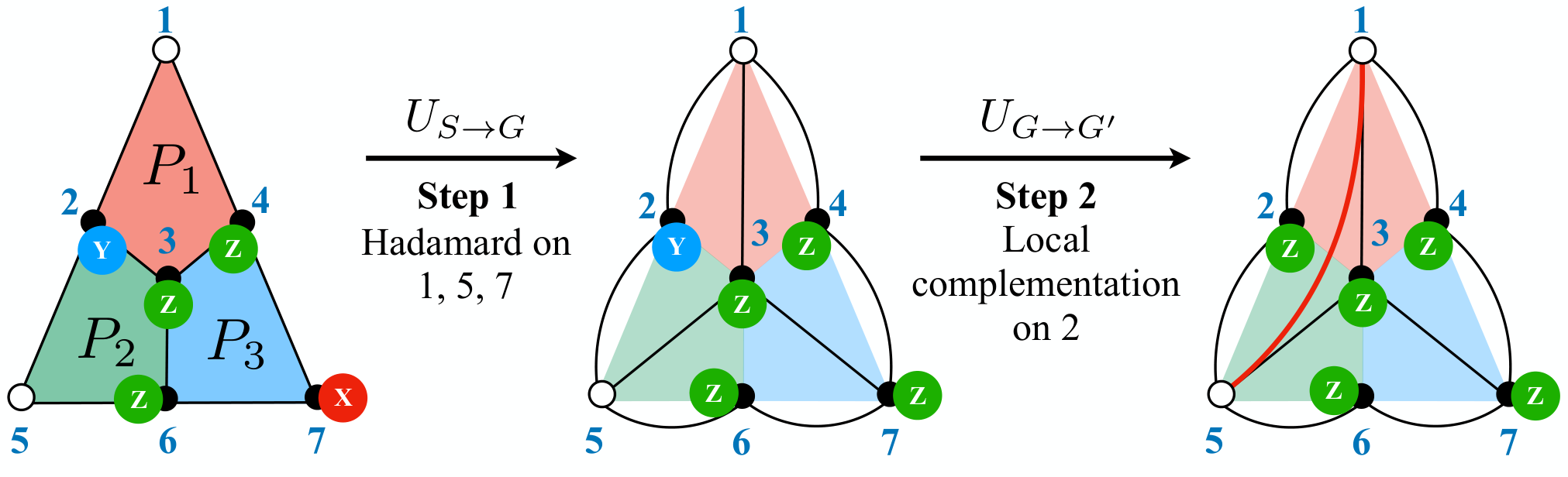
Appendix F Graph-based algorithm on a 7-qubit color code
The graph-based method for computing the measurement-based lower bound of LE has been discussed in Sec. II.2. In this appendix, for illustration, we apply the graph-based method described in Sec. II.2 on the smallest 2D color code, constructed over a triangular lattice of seven qubits arranged in three adjoined plaquettes, where one physical qubit is placed at each vertex. The stabilizer operators corresponding to the 7-qubit color code are constituted of 4-qubit - and -type operators for each plaquette, given by
| (88) |
Let us assume that the two-qubit region is given by the qubits and (see Fig. 14), where . The logical state of this TCC can be transformed into a graph state via the unitary transformation , where the set of control qubits here is composed of the qubits , and the set of targets holds the qubits . The link is absent in the graph . Therefore, a subsequent LC operation on the qubit is performed to create the graph , where the link exists. This LC transformation is equivalent to (see Appenndix D). Therefore, the unitary operator consists of the local unitary operators , , and in the region . Consequently, as a MLB with measurement on all qubits in is equivalent to measurement on qubit , measurement on qubit , and measurements on qubits , , and , denoted altogether by in , so that .
Appendix G Graph transformations via Adaptive Local Complementation
As mentioned in Sec. II.2, for the successful implementation of the graph-based protocol, one needs to develop a graph trannsformation algorithm that creates a link between any two chosen nodes in a simple, connected, undirected graph via a sequence of local complementation operations over a set of nodes in the graph. We have developed an adaptive local complementation technique that updates itself at every step of the graph transformation via local complementation over one qubit, and chooses the next node for local complementation using the updated information. Here, we discuss the technical details of the adaptive LC technique developed for the graph transformation used in Sec. II.2. The prescription works for a generic simple, connected, and undirected graph , irrespective of whether it is bicolorable or not.
We shall denote a link connecting two nodes and by . We shall also represent a simple path in the graph, connecting the two nodes and and having length , by , which, without any loss in generality, is given by (see Appendix D)
| (89) |
Here, are the nodes that are visited while traveling from to along , such that , , and none of the nodes is repeated in the sequence. The number of links traversed while going from to is the length of the path. To keep the notation uncluttered, we will drop the subscript and the superscript from the notation of the simple path unless it is explicitly required for comparison. For the purpose of this discussion, one needs a specific classification of the simple paths connecting two nodes, and a definition of the distance between them, as follows.
Category of simple paths. We first divide the set of all possible simple paths between two given nodes and into two categories, and . A simple path of the form given in Eq. (89) belongs to the category if a qubit on is not connected to another qubit on via a direct link, unless the second qubit is right before or after the first qubit in the sequence . Formally put, for two qubits and on , iff , , , then . Otherwise, (see Fig. 15 for an example). Note that , while constitutes the set of all possible simple paths between and .
Distance between two nodes. There can be a number of ways in which the distance between a pair of nodes in a graph can be quantified. However, the distance between two nodes and that is specific to a given path of the form in Eq. (89) is unique. It is measured by the number of links that one has to traverse while going from to along , and can be represented by , where we have assumed without any loss of generality. Note that for a path , .
All shortest paths between two given nodes and in a simple, connected, and undirected graph belongs to . This can be proved by assuming that there exists a shortest path (see Appendix D for a definition) between two nodes and that belongs to . However, by definition of , there exists at least one link such that , , and . This implies that there exists a simple path between and , given by
of length , which is since by the definition of . Therefore, is not a shortest path. However, note that not all paths in are shortest paths (see Fig. 15 for examples).
We are now in a position to prove the following Theorem, which will be crucial for our purpose.
Theorem 1. For a simple path of the form given in Eq. (89) between a pair of nodes and in a graph , a sequence of LC operations on the nodes always creates a link between the nodes and , when the LC operations are performed on the nodes in the same order as they are in the sequence .
Proof. Let us consider the path , as given in Eq. (89), between the nodes and in a simple, connected, and undirected graph . Let us denote the neighborhood of the node as . The definition of implies that only belongs to , while . Let us assume that the LC operation (see Appendix D) on node transforms the graph as . The definition of LC operation implies creation of the link thereby introducing in the neighborhood of , while keeping the neighborhoods of the rest of the nodes unchanged. Also, the LC operation does not affect the links , . Therefore, in , there exists a simple path of length , given by , between the pair of nodes and . One can continue performing a total of LC operations successively on the nodes in the same order as they are in the sequence , where during each individual LC operations on the node , , the above arguments apply, and a link is created between the node and the node . The last LC operation on the node creates a link between the nodes and . Hence the proof.
Corollary 1.1. For a shortest path of the form given in Eq. (89) between a pair of nodes and in a graph , a sequence of LC operations on the nodes always creates a link between the nodes and , when the LC operations are performed on the nodes in the same order as they are in the sequence .
Corollary 1.2. For a path of length , the number of LC operations required to create the link is .
Theorem 1 suggests that the creation of a link between and in a connected graph is ensured if one chooses only paths between and and perform LC operations on the qubits in those paths. However, there usually exists a large number of paths in a connected graph, and there is no intuition whatsoever for choosing a path in order to obtain a tight MLB of LE. The challenge therefore is to develop an effective algorithm that can guarantee the creation of the link irrespective of whether the chosen path belongs to or , when LC operations only on the nodes belonging to the chosen path are performed. Towards this goal, note that by virtue of the definition of , for a path , one can distil a number of paths of different lengths from the links constructing and the links connecting the nodes in the , but not contributing to (see Fig. 15 for examples). These paths have support on the nodes only, and therefore the condition of performing LC operations only on the nodes belonging to is satisfied. Theorem 1 ensures that each of these paths can be chosen to create with certainty. Therefore, the challenge is to find a path from the path, which, in turn, leads to the creation of the link according to Theorem 1. It is easily understood how this is achieved via the algorithm represented by the pseudocode in Appendix H.4.
Note here that to minimize effort, one has to use the distilled path having the shortest length, which may or may not be the shortest path between and . However, there is no intuitive reason behind using the shortest path, or the shortest distilled path to create the link, since the value of the MLB computed via the graph-based method I depends explicitly on the structure of the graph, and how the size of the neighborhood of the qubit-pair in the transformed graph depends on the length of the chosen path between and in the original graph. In a graph with high connectivity, there may exist other paths having length close to the shortest length which may provide a tighter value of the MLB compared to the same obtained from the shortest path (we elaborate more on this in Sec. IV). The algorithm focuses on finding any one of the distilled paths that creates the link . For example, in Fig. 15, the algorithm distils the path of length , while the shortest distilled path is of length , which is also one of the shortest paths between the qubits and .
We now combine all these insights, and develop an LC-based graph-transformation algorithm that creates a link by performing LC operations on a subset of the set of nodes situated on a chosen path, where the subset of nodes is chosen by adapting the chosen path according to its category. We call this algorithm the Adaptive LC (ALC) algorithm, which has been represented by the pseudocode in Appendix H.5. The LC operation on a simple, connected, and undirected graph w.r.t. a chosen node, the distillation of a path from a path via the algorithm, and the creation of a link between any two given nodes in a graph by using ALC algorithm have been realized in the form of the Python open-source package ALCPack Amaro et al. 2019.
A word on the dependence of the run-time of the adaptive LC algorithm on the system size is in order here. Since the algorithm takes into account the transformed graphs at each of its steps, it is difficult to determine an exact dependence of the run-time of the algorithm on system size. However, one can determine a bound on how the run-time scales with . It is easy to see that the maximum size of the neighborhood of a node can be , and it can host at most links if is connected and undirected. Therefore, the maximum number of links that can be created or deleted during an LC operation on a single node is . Since there can be at most nodes on a path between and , the total number of link operations during the ALC algorithm is , which indicates a polynomial scaling with system size.
Appendix H Pseudo codes for different algorithms
In this Appendix, we present pseudo-codes for the different algorithms introduced in this paper.
H.1 Graph-based method
We now present the pseudo code representing the graph-based method to calculate the measurement-based lower bound for localizable entanglement.
input (1) on system of size , (2) qubit-pair , and (3) noise map
- 1.
obtain and corresponding to all
- 2.
for all , do
- (a)
if link then
- i.
for all , do
- A.
perform the transformation via adaptive local complementations on
- B.
determine
- C.
determine noise transformation
- D.
due to
- E.
compute following Amaro et al. 2018
- F.
determine
- A.
- i.
- (b)
else
- i.
determine due to
- ii.
compute following Amaro et al. 2018
- iii.
determine
- i.
- (a)
output (1) , and (2) measurement setup
H.2 Modified graph-based method
The graph-based method will be modified if the graph obtained from the stabilizer state already has a link between the chosen qubits. The modified algorithm is as follows.
input (1) on system of size , (2) qubit-pair , and (3) noise map
- 1.
obtain and corresponding to all such that
- 2.
for all , do
- (a)
determine due to
- (b)
compute following Amaro et al. 2018
- (c)
determine
- (a)
output (1) , (2) measurement setup
H.3 Determination of the adjacency matrix
The following pseudo code is for obtaining the adjacency matrix of bicolorable graphs from the stabilizer states as per the algebraic approach discussed in Appendix E. Note that similar code has been used to develop the Stabgraph package.
input Stabilizer state in the binary representation as given in Eq. (44)
- 1.
obtain via Gauss elimination on
- 2.
determine in bottom block via reordering rows
- 3.
apply same reordering in top block to get in Eq. (E)
- 4.
identify ,,, from
- 5.
- 6.
construct (Eq. (E))
output adjacency matrix describing a graph state which is local unitary equivalent to the input stabilizer state.
H.4 Obtaining a path from a path
We now present the algorithm developed in Appendix G to convert a category path to a category path.
input (1) graph , (2) qubit-pair such that , and (3) a path between
initiate list of nodes
- 1.
determine : neighborhood of
- 2.
determine
- 3.
determine node with maximum
- 4.
append to
- 5.
if then
- (a)
- (b)
repeat 1-5
- (a)
- 6.
else
-
stop
-
output connecting
H.5 Adaptive local complementation
We can now adapt the pseudo codes discussed in Appendix H.4 and obtain an adaptive local complementation algorithm, as follows. This also is the underlying algorithm for the ALCPack.
input (1) graph , and (2) qubit-pair such that and there exists a simple path connecting and
- 1.
determine category of
- 2.
if then
- (a)
apply algorithm and determine the shortest path
- (b)
- (a)
- 3.
perform local complementation operations on nodes belonging to in same sequence as
output transformed graph ,
Appendix I Graphs from color codes: Illustration
In this appendix, we demonstrate the procedure for obtaining a graph state from a topological color code with an example. In the case of a four-qubit plaquette in a topological color code, constituted of four qubits , , , and , the first step is to initialize the four qubits in the product state , and then to apply CNOT gates successively over the qubit-pairs , , and , always using qubit as the control qubit. This leads to the four-qubit GHZ state
over the plaquette . Here, the CNOT operator is given by
| (92) |
for a qubit-pair , where denotes the control and denotes a target qubit. The state can be further transformed to a graph state corresponding to a simple, connected, and undirected star-shaped graph with the control qubit as the central qubit via local unitary transformations on the target qubits Hein et al. 2006, where represents a Hadamard operator (see Fig. 5). Note here that the convention of creating the graph state involves initializing all the qubits in , and subsequently applying a controlled phase gate on all pairs of nodes Hein et al. 2006, where the controlled phase gate,
| (93) |
is connected to via a Hadamard operation on the target qubit: . In terms of the stabilizer operators, the plaquette stabilizer is transformed to the graph-state generator via application of Hadamard operations on the target qubits.
Appendix J Binary picture
Here we provide a few essential details on the binary picture of the stabilizer formalism Hein et al. 2006.
Pauli operators. In the binary picture, the single-qubit identity and Pauli operators are represented by the column vectors
and the products of these operators are mapped to the sum of the columns modulo . Note that in the binary picture, the global phases are disregarded.
Clifford operations. Single-qubit Clifford operators are binary matrices that multiply from the left to the Pauli operators given in Eq. (). Given that these operators do not transform Pauli matrices into the identity, their representative binary matrix is full-rank. As an examples, the Hadamard gate and a -rotation are represented by
One can check that interchanges and , while changes to .
Stabilizer state. A stabilizer state of qubits is represented by a binary matrix formed by two blocks,
| (109) |
where the -th stabilizer is represented by the -th column, and the qubit is represented by the rows and in such a way that the column of two elements, written as
| (110) |
represents the operator from the set that is applied to the qubit due to stabilizer . For example, the two-qubit maximally entangled state defined by the stabilizers and is represented by
| (111) |
Another important example is a graph state defined on an underlying graph represented by the adjacency matrix . The stabilizer description of the graph state is given in Appendix D. Given that the neighborhood of qubit includes the nodes corresponding to the non-vanishing elements of the -th column of , the representation of a graph state is completely defined by the adjacency matrix as
| (112) |
where is the identity matrix. In a stabilizer state, all stabilizers are independent, implying that no product of them exists which equals to the identity operator. Since in the binary picture the product of Pauli operators is mapped to a sum of columns, all the columns of must be linearly independent, or equivalently, . Moreover, an invertible recombination of the stabilizers operators leads to the same stabilizer operator. In the binary picture this recombination is represented by an invertible binary matrix that multiplies from the right. Finally, the commutation of the stabilizer operators defining a stabilizer state is guaranteed by the relation , where is the matrix:
| (113) |
Clifford operation on stabilizer state. Clifford operations performed on multiple qubits of the stabilizer state are represented by binary matrices that multiply from the left. Clifford operations can not map a stabilizer operator or a recombination of them into the identity operator, implying that multiplication of to for all can not result in vanishing a column. Consequently, is a full-rank matrix. For local operations like or in Eq. (J), is the tensor product of the single-qubit matrices. For example,
| (114) |
represents a -rotation applied on every qubits for which , being a diagonal matrix.
Appendix K Uncorrelated single-qubit Pauli noise
We consider an operator-sum representation Holevo and Giovannetti 2012; Nielsen and Chuang 2010 of the uncorrelated single-qubit Pauli noise applied to the stabilizer state , given by , where
| (115) |
Here, are the Kraus operators satisfying the completeness condition , and is a probability distribution, representing the strength of the noise. The individual operators, can be written as
| (116) |
whereas
| (117) |
with , , and , , , and . Here we interpret the index as the multi-index , where the value of is the decimal representation of the base string . Examples of uncorrelated Pauli noise include phase-flip (, , ) , bit-flip (, , ), bit-phase-flip (, , ), and depolarizing (, ) noises.
Appendix L Stabilizer expectation values under noise
For the purpose of demonstration, we choose the phase-flip noise, where due to the specific values of the probabilities , only terms in the sum in Eq. (115) survive. We rewrite Eq. (115) for the PF noise as
| (118) |
where the index has similar definition as before, only with , , and , . From the form of the Kraus operators and the fact that , it is easy to see that . However, in the case of ,
| (119) |
Writing and , where is the set of qubits constructing the support of such that constructs the entire system, and , with () defined similarly as for qubits in (), Eq. (119) becomes
| (120) |
since the probabilities sum up to 1. The form of suggests that the value of the trace in the parenthesis in Eq. (120) is if the number of qubits in for which is even (odd). Using the explicit forms of in terms of for the PF noise (see Appendix K), Eq. (120) yields
| (121) |
which, upon using the identities
leads to
| (123) |
Lastly, using the commutation of and , it is easy to show that .
We point out here that the calculation for the bit-flip and the depolarizing channels would be exactly similar to the same for the phase-flip channel. However, in the case of the depolarizing channel, all terms in the operator-sum representation have to be considered.
References
- Bennett and DiVincenzo (2000) C. H. Bennett and D. P. DiVincenzo, Nature 404, 247 (2000).
- Horodecki et al. (2009) R. Horodecki, P. Horodecki, M. Horodecki, and K. Horodecki, Rev. Mod. Phys. 81, 865 (2009).
- Bennett et al. (1993) C. H. Bennett, G. Brassard, C. Crépeau, R. Jozsa, A. Peres, and W. K. Wootters, Phys. Rev. Lett. 70, 1895 (1993).
- Bouwmeester et al. (1997) D. Bouwmeester, J.-W. Pan, K. Mattle, M. Eibl, H. Weinfurter, and A. Zeilinger, Nature 390, 575 (1997).
- Bennett and Wiesner (1992) C. H. Bennett and S. J. Wiesner, Phys. Rev. Lett. 69, 2881 (1992).
- Mattle et al. (1996) K. Mattle, H. Weinfurter, P. G. Kwiat, and A. Zeilinger, Phys. Rev. Lett. 76, 4656 (1996).
- Sen (De) A. Sen(De) and U. Sen, Phys. News 40, 17 (2011), arXiv:1105.2412 .
- Ekert (1991) A. K. Ekert, Phys. Rev. Lett. 67, 661 (1991).
- Jennewein et al. (2000) T. Jennewein, C. Simon, G. Weihs, H. Weinfurter, and A. Zeilinger, Phys. Rev. Lett. 84, 4729 (2000).
- Raussendorf and Briegel (2001) R. Raussendorf and H. J. Briegel, Phys. Rev. Lett. 86, 5188 (2001).
- Raussendorf et al. (2003) R. Raussendorf, D. E. Browne, and H. J. Briegel, Phys. Rev. A 68, 022312 (2003).
- Briegel et al. (2009) H. J. Briegel, D. E. Browne, W. Dür, R. Raussendorf, and M. Van den Nest, Nat. Phys. 5, 19 (2009).
- Pollmann et al. (2010) F. Pollmann, A. M. Turner, E. Berg, and M. Oshikawa, Phys. Rev. B 81, 064439 (2010).
- Chen et al. (2010) X. Chen, Z.-C. Gu, and X.-G. Wen, Phys. Rev. B 82, 155138 (2010).
- Jiang et al. (2012) H.-C. Jiang, Z. Wang, and L. Balents, Nat. Phys. 8, 902 (2012).
- Osterloh et al. (2002) A. Osterloh, L. Amico, G. Falci, and R. Fazio, Nature 416, 608 (2002).
- Osborne and Nielsen (2002) T. J. Osborne and M. A. Nielsen, Phys. Rev. A 66, 032110 (2002).
- Amico et al. (2008) L. Amico, R. Fazio, A. Osterloh, and V. Vedral, Rev. Mod. Phys. 80, 517 (2008).
- Chiara and Sanpera (2018) G. D. Chiara and A. Sanpera, Rep. Prog. Phys. 81, 074002 (2018).
- Sarovar et al. (2010) M. Sarovar, A. Ishizaki, G. R. Fleming, and K. B. Whaley, Nat. Phys. 6, 462 (2010).
- Zhu et al. (2012) J. Zhu, S. Kais, A. Aspuru-Guzik, S. Rodriques, B. Brock, and P. J. Love, J. Chem. Phys. 137, 074112 (2012).
- Lambert et al. (2013) N. Lambert, Y.-N. Chen, Y. Cheng, C.-M. Li, G. Chen, and F. Nori, Nat. Phys. 9, 10 (2013).
- Chanda et al. (2014) T. Chanda, U. Mishra, A. Sen(De), and U. Sen, arXiv:1412.6519 (2014).
- Cai et al. (2010) J. Cai, G. G. Guerreschi, and H. J. Briegel, Phys. Rev. Lett. 104, 220502 (2010).
- Hubeny (2015) V. E. Hubeny, Classical Quant. Grav. 32, 124010 (2015).
- Pastawski et al. (2015) F. Pastawski, B. Yoshida, D. Harlow, and J. Preskill, J. High. Energy Phys. 2015, 149 (2015).
- Almheiri et al. (2015) A. Almheiri, X. Dong, and D. Harlow, J. High Energy Phys. 4, 163 (2015).
- Jahn et al. (2017) A. Jahn, M. Gluza, F. Pastawski, and J. Eisert, arXiv:1711.03109 (2017).
- Leibfried et al. (2003) D. Leibfried, R. Blatt, C. Monroe, and D. Wineland, Rev. Mod. Phys. 75, 281 (2003).
- Leibfried et al. (2005) D. Leibfried, E. Knill, S. Seidelin, J. Britton, R. B. Blakestad, J. Chiaverini, D. B. Hume, W. M. Itano, J. D. Jost, C. Langer, R. Ozeri, R. Reichle, and D. J. Wineland, Nature 438, 639 (2005).
- Brown et al. (2016) K. R. Brown, J. Kim, and C. Monroe, Nature Phys. J. Quant. Inf. 2, 16034 EP (2016).
- Raimond et al. (2001) J. M. Raimond, M. Brune, and S. Haroche, Rev. Mod. Phys. 73, 565 (2001).
- Prevedel et al. (2009) R. Prevedel, G. Cronenberg, M. S. Tame, M. Paternostro, P. Walther, M. S. Kim, and A. Zeilinger, Phys. Rev. Lett. 103, 020503 (2009).
- Barz (2015) S. Barz, J. Phys. B 48, 083001 (2015).
- Negrevergne et al. (2006) C. Negrevergne, T. S. Mahesh, C. A. Ryan, M. Ditty, F. Cyr-Racine, W. Power, N. Boulant, T. Havel, D. G. Cory, and R. Laflamme, Phys. Rev. Lett. 96, 170501 (2006).
- Clarke and Wilhelm (2008) J. Clarke and F. K. Wilhelm, Nature 453, 1031 (2008).
- Berkley et al. (2003) A. J. Berkley, H. Xu, R. C. Ramos, M. A. Gubrud, F. W. Strauch, P. R. Johnson, J. R. Anderson, A. J. Dragt, C. J. Lobb, and F. C. Wellstood, Science 300, 1548 (2003).
- Hald et al. (1999) J. Hald, J. L. Sørensen, C. Schori, and E. S. Polzik, Phys. Rev. Lett. 83, 1319 (1999).
- Mandel et al. (2003) O. Mandel, M. Greiner, A. Widera, T. Rom, T. W. Hansch, and I. Bloch, Nature 425, 937 (2003).
- Bloch (2005) I. Bloch, J. Phys. B: At. Mol. Opt. Phys. 38, S629 (2005).
- Bloch et al. (2008) I. Bloch, J. Dalibard, and W. Zwerger, Rev. Mod. Phys. 80, 885 (2008).
- Bernien et al. (2013) H. Bernien, B. Hensen, W. Pfaff, G. Koolstra, M. S. Blok, L. Robledo, T. H. Taminiau, M. Markham, D. J. Twitchen, L. Childress, and R. Hanson, Nature 497, 86 (2013).
- Togan et al. (2010) E. Togan, Y. Chu, A. S. Trifonov, L. Jiang, J. Maze, L. Childress, M. V. G. Dutt, A. S. Sørensen, P. R. Hemmer, A. S. Zibrov, and M. D. Lukin, Nature 466, 730 (2010).
- Marinković et al. (2018) I. Marinković, A. Wallucks, R. Riedinger, S. Hong, M. Aspelmeyer, and S. Gröblacher, Phys. Rev. Lett. 121, 220404 (2018).
- DiVincenzo (2000) D. P. DiVincenzo, Fortschr. Phys. 48, 771 (2000).
- Gottesman (2010) D. Gottesman, in Quantum information science and its contributions to mathematics, Proceedings of Symposia in Applied Mathematics, Vol. 68 (2010) pp. 13–58.
- Benhelm et al. (2008) J. Benhelm, G. Kirchmair, C. F. Roos, and R. Blatt, Nat. Phys. 4, 463 (2008).
- Chow et al. (2012) J. M. Chow, J. M. Gambetta, A. D. Córcoles, S. T. Merkel, J. A. Smolin, C. Rigetti, S. Poletto, G. A. Keefe, M. B. Rothwell, J. R. Rozen, M. B. Ketchen, and M. Steffen, Phys. Rev. Lett. 109, 060501 (2012).
- Barends et al. (2014) R. Barends, J. Kelly, A. Megrant, A. Veitia, D. Sank, E. Jeffrey, T. C. White, J. Mutus, A. G. Fowler, B. Campbell, Y. Chen, Z. Chen, B. Chiaro, A. Dunsworth, C. Neill, P. O’Malley, P. Roushan, A. Vainsencher, J. Wenner, A. N. Korotkov, A. N. Cleland, and J. M. Martinis, Nature 508, 500 (2014).
- Preskill (2018) J. Preskill, Quantum 2, 79 (2018).
- Paler et al. (2018) A. Paler, A. Zulehner, and R. Wille, arXiv:1806.07241 (2018).
- Nash et al. (2019) B. Nash, V. Gheorghiu, and M. Mosca, arXiv:1904.01972 (2019).
- Preskill (2012) J. Preskill, arXiv:1203.5813 (2012).
- Fujii (2015) K. Fujii, arXiv:1504.01444 (2015).
- Ibort et al. (2009) A. Ibort, V. I. Man’ko, G. Marmo, A. Simoni, and F. Ventriglia, Physica Scripta 79, 065013 (2009).
- Lvovsky and Raymer (2009) A. I. Lvovsky and M. G. Raymer, Rev. Mod. Phys. 81, 299 (2009).
- Huang (2014) Y. Huang, New Journal of Physics 16, 033027 (2014).
- Nayak et al. (2008) C. Nayak, S. H. Simon, A. Stern, M. Freedman, and S. Das Sarma, Rev. Mod. Phys. 80, 1083 (2008).
- Pachos and Simon (2014) J. K. Pachos and S. H. Simon, New J. Phys. 16, 065003 (2014).
- Lahtinen and Pachos (2017) V. Lahtinen and J. K. Pachos, SciPost Phys. 3, 021 (2017).
- Dennis et al. (2002) E. Dennis, A. Kitaev, A. Landahl, and J. Preskill, J. Math. Phys. 43, 4452 (2002).
- Kitaev (2006) A. Kitaev, Ann. Phys. 321, 2 (2006).
- Bombin and Martin-Delgado (2006) H. Bombin and M. A. Martin-Delgado, Phys. Rev. Lett. 97, 180501 (2006).
- Bombin and Martin-Delgado (2007) H. Bombin and M. A. Martin-Delgado, Phys. Rev. Lett. 98, 160502 (2007).
- Dusuel et al. (2011) S. Dusuel, M. Kamfor, R. Orús, K. P. Schmidt, and J. Vidal, Phys. Rev. Lett. 106, 107203 (2011).
- Jahromi et al. (2013) S. S. Jahromi, M. Kargarian, S. F. Masoudi, and K. P. Schmidt, Phys. Rev. B 87, 094413 (2013).
- Zarei (2015) M. H. Zarei, Phys. Rev. A 91, 022319 (2015).
- Jamadagni et al. (2018) A. Jamadagni, H. Weimer, and A. Bhattacharyya, Phys. Rev. B 98, 235147 (2018).
- Stace et al. (2009) T. M. Stace, S. D. Barrett, and A. C. Doherty, Phys. Rev. Lett. 102, 200501 (2009).
- Stace and Barrett (2010) T. M. Stace and S. D. Barrett, Phys. Rev. A 81, 022317 (2010).
- Vodola et al. (2018) D. Vodola, D. Amaro, M. A. Martin-Delgado, and M. Müller, Phys. Rev. Lett. 121, 060501 (2018).
- Katzgraber et al. (2009) H. G. Katzgraber, H. Bombin, and M. A. Martin-Delgado, Phys. Rev. Lett. 103, 090501 (2009).
- Nigg et al. (2014) D. Nigg, M. Müller, E. A. Martinez, P. Schindler, M. Hennrich, T. Monz, M. A. Martin-Delgado, and R. Blatt, Science 345, 302 (2014).
- Linke et al. (2017) N. M. Linke, M. Gutierrez, K. A. Landsman, C. Figgatt, S. Debnath, K. R. Brown, and C. Monroe, Sci. Adv. 3, 10 (2017).
- Wright et al. (2019) K. Wright, K. M. Beck, S. Debnath, J. M. Amini, Y. Nam, N. Grzesiak, J.-S. Chen, N. C. Pisenti, M. Chmielewski, C. Collins, K. M. Hudek, J. Mizrahi, J. D. Wong-Campos, S. Allen, J. Apisdorf, P. Solomon, M. Williams, A. M. Ducore, A. Blinov, S. M. Kreikemeier, V. Chaplin, M. Keesan, C. Monroe, and J. Kim, arXiv:1903.08181 (2019).
- Kelly et al. (2015) J. Kelly, R. Barends, A. G. Fowler, A. Megrant, E. Jeffrey, T. C. White, D. Sank, J. Y. Mutus, B. Campbell, Y. Chen, Z. Chen, B. Chiaro, A. Dunsworth, I.-C. Hoi, C. Neill, P. J. J. O’Malley, C. Quintana, P. Roushan, A. Vainsencher, J. Wenner, A. N. Cleland, and J. M. Martinis, Nature 519, 66 (2015).
- Gambetta et al. (2017) J. M. Gambetta, J. M. Chow, and M. Steffen, Nature Phys. J. Quant. Inf. 3, 2 (2017).
- Castelnovo and Chamon (2007) C. Castelnovo and C. Chamon, Phys. Rev. B 76, 184442 (2007).
- Castelnovo and Chamon (2008) C. Castelnovo and C. Chamon, Phys. Rev. B 78, 155120 (2008).
- Schmitz et al. (2019) A. T. Schmitz, S.-J. Huang, and A. Prem, Phys. Rev. B 99, 205109 (2019).
- DiVincenzo et al. (1998) D. P. DiVincenzo, C. A. Fuchs, H. Mabuchi, J. A. Smolin, A. Thapliyal, and A. Uhlmann, arXiv:quant-ph/9803033 (1998).
- Verstraete et al. (2004a) F. Verstraete, M. Popp, and J. I. Cirac, Phys. Rev. Lett. 92, 027901 (2004a).
- Popp et al. (2005) M. Popp, F. Verstraete, M. A. Martín-Delgado, and J. I. Cirac, Phys. Rev. A 71, 042306 (2005).
- Sadhukhan et al. (2017) D. Sadhukhan, S. S. Roy, A. K. Pal, D. Rakshit, A. Sen(De), and U. Sen, Phys. Rev. A 95, 022301 (2017).
- Kitaev and Preskill (2006) A. Kitaev and J. Preskill, Phys. Rev. Lett. 96, 110404 (2006).
- Levin and Wen (2006) M. Levin and X.-G. Wen, Phys. Rev. Lett. 96, 110405 (2006).
- Linke et al. (2018) N. M. Linke, S. Johri, C. Figgatt, K. A. Landsman, A. Y. Matsuura, and C. Monroe, Phys. Rev. A 98, 052334 (2018).
- Brydges et al. (2019) T. Brydges, A. Elben, P. Jurcevic, B. Vermersch, C. Maier, B. P. Lanyon, P. Zoller, R. Blatt, and C. F. Roos, Science 364, 260 (2019).
- Kitaev (2003) A. Kitaev, Ann. Phys. 303, 2 (2003).
- Kargarian (2008) M. Kargarian, Phys. Rev. A 78, 062312 (2008).
- Van den Nest et al. (2004) M. Van den Nest, J. Dehaene, and B. De Moor, Phys. Rev. A 69, 022316 (2004).
- Hein et al. (2006) M. Hein, W. Dür, J. Eisert, R. Raussendorf, M. Van den Nest, and H. J. Briegel, arXiv:quant-ph/0602096 (2006).
- Amaro et al. (2018) D. Amaro, M. MÃŒller, and A. K. Pal, New J. Phys. 20, 063017 (2018).
- Verstraete et al. (2004b) F. Verstraete, M. A. Martín-Delgado, and J. I. Cirac, Phys. Rev. Lett. 92, 087201 (2004b).
- Jin and Korepin (2004) B.-Q. Jin and V. E. Korepin, Phys. Rev. A 69, 062314 (2004).
- Skrøvseth and Bartlett (2009) S. O. Skrøvseth and S. D. Bartlett, Phys. Rev. A 80, 022316 (2009).
- Smacchia et al. (2011) P. Smacchia, L. Amico, P. Facchi, R. Fazio, G. Florio, S. Pascazio, and V. Vedral, Phys. Rev. A 84, 022304 (2011).
- Montes and Hamma (2012) S. Montes and A. Hamma, Phys. Rev. E 86, 021101 (2012).
- Acín et al. (2007) A. Acín, J. I. Cirac, and M. Lewenstein, Nat. Phys. 3, 256 (2007).
- Terhal (2002) B. M. Terhal, Theor. Comput. Sci. 287, 313 (2002).
- Gühne et al. (2002) O. Gühne, P. Hyllus, D. Bruß, A. Ekert, M. Lewenstein, C. Macchiavello, and A. Sanpera, Phys. Rev. A 66, 062305 (2002).
- Bourennane et al. (2004) M. Bourennane, M. Eibl, C. Kurtsiefer, S. Gaertner, H. Weinfurter, O. Gühne, P. Hyllus, D. Bruß, M. Lewenstein, and A. Sanpera, Phys. Rev. Lett. 92, 087902 (2004).
- Gühne and Tóth (2009) O. Gühne and G. Tóth, Phys. Rep. 474, 1 (2009).
- Tóth and Gühne (2005) G. Tóth and O. Gühne, Phys. Rev. A 72, 022340 (2005).
- Alba et al. (2010) E. Alba, G. Tóth, and J. J. García-Ripoll, Phys. Rev. A 82, 062321 (2010).
- Friis et al. (2018) N. Friis, O. Marty, C. Maier, C. Hempel, M. Holzäpfel, P. Jurcevic, M. B. Plenio, M. Huber, C. Roos, R. Blatt, and B. Lanyon, Phys. Rev. X 8, 021012 (2018).
- Amaro and Müller (2019) D. Amaro and M. Müller, arXiv:1911.01144 (2019).
- Lang and Büchler (2012) N. Lang and H. P. Büchler, Phys. Rev. A 86, 022336 (2012).
- Brandão (2005) F. G. S. L. Brandão, Phys. Rev. A 72, 022310 (2005).
- Brandão and Viana (2006) F. G. S. L. Brandão and R. O. Viana, Int. J. Quant. Inf. 04, 331 (2006).
- Eisert et al. (2007) J. Eisert, F. G. S. L. Brandão, and K. M. R. Audenaert, New J. Phys. 9, 46 (2007).
- Gühne et al. (2007) O. Gühne, M. Reimpell, and R. F. Werner, Phys. Rev. Lett. 98, 110502 (2007).
- Gühne et al. (2008) O. Gühne, M. Reimpell, and R. F. Werner, Phys. Rev. A 77, 052317 (2008).
- Amaro (2019) D. Amaro, “stabgraph,” availale at https://github.com/davamaro/stabgraph (2019).
- Amaro et al. (2019) D. Amaro, M. Müller, and A. K. Pal, “alcpack,” available at https://github.com/amitkpal/alcpack (2019).
- Peres (1996) A. Peres, Phys. Rev. Lett. 77, 1413 (1996).
- Horodecki et al. (1996) M. Horodecki, P. Horodecki, and R. Horodecki, Phys. Lett. A 223, 1 (1996).
- Greenberger et al. (1989) D. M. Greenberger, M. A. Horne, and A. Zeilinger, Bell’s theorem, quantum theory and conceptions of the universe (Kluwer, Netherlands, 1989).
- Nielsen and Chuang (2010) M. A. Nielsen and I. L. Chuang, Quantum Computation and Quantum Information (Cambridge University Press, 2010).
- Holevo and Giovannetti (2012) A. S. Holevo and V. Giovannetti, Rep. Prog. Phys. 75, 046001 (2012).