Quantum mechanics and speed limit of ultrafast local control in spin chains
Abstract
We study optimization of fidelity for ultrafast transformation of a spin chain via external control of a local exchange coupling. We show that infidelity of such a process can be dramatically decreased by choosing a proper control profile in nonadiabatic time domain, predict main features of this profile analytically, corroborate them numerically with a gradient search algorithm, and discuss the corresponding quantum speed limit. For ultrafast transformations, the qualitative features of the obtained optimal control are system-independent. Moreover, the main restrictions on its shape do not depend on the transformation time and remain valid up to the adiabatic limit. Our results can be applied to control a broad variety of quantum systems.
I Introduction
Recent progress in experimental research on quantum systems described by moderate-size Hilbert spaces, such as ensembles of qubits, posed fascinating problems of optimal quantum control Peirce et al. 1988; Brif et al. 2010; Borzi et al. 2017; Caneva et al. 2011a; Caneva et al. 2014 of these systems. The quantum control aims at achieving desired quantum states or certain quantum operations with maximum possible fidelity using limited resources such as time or energy. The dynamics of quantum systems under external control can be unitary or non-unitary. The unitary dynamics is driven by a time-dependent controllable Hamiltonian , where is a multicomponent control function. The controllable non-unitary dynamics is achievable by system measurements Li et al. 2011; Luchnikov and Filippov 2017; Wu et al. 2004; Pyshkin et al. 2016; Torres et al. 2017, via a controllable interaction with a non-Markovian environment Verstraete et al. 2009; Jing and Yu 2010; Luo et al. 2015 or via control of the unitary part of the evolution of open system Schmidt et al. 2011.
We consider driving a quantum system from a ground state of initial Hamiltonian to achieve at time ground state of a final Hamiltonian with where and Although a high fidelity can be obtained by an adiabatic process Born and Fock 1928 driven by a slowly varying with, e.g., , this method requires a long evolution while optimized can permit achieving a demanded quantum state for a relatively short
A possible approach to the quantum control, where the transitions occur between the ground states of , is based on the shortcut to adiabaticity Torrontegui et al. 2013; Guéry-Odelin et al. 2019; Demirplak and Rice 2003; Berry 2009; Ren et al. 2017. However, this technique requires a control of the all parts of a complex quantum system. Implementation of a such a shortcut can be a part of quantum computation in arrays of quantum dots Loss and DiVincenzo 1998; Burkard et al. 1999, or in quantum annealing Das and Chakrabarti 2008, such as applied in D-Wave computer McGeoch 2014. Here by focusing on high fidelity ultrafast processes, we analytically obtain properties of optimal local control in the ultra-short time domain for a particular many-body system and corroborate our reasoning by a direct numerical optimization. We show that several properties of the finite time quantum control (even for the ultra-short time) can be explained by requiring a smooth passage to the adiabatic protocols, thus, connecting these two limits. Although the reported results are obtained for spin chains, the proposed heuristic reasoning and numerical approach can be extended to a much broader class of quantum systems.

II Ultrafast local control: the problem setting
We concentrate on a local control acting only on a small part of a complex system, being a natural tool for cutting or stitching links between its parts, thus, modifying its size and/or topology. We consider an Ising chain with spins, as shown in Fig. 1, described by the Hamiltonian
| (1) |
where are corresponding Pauli matrices of the -th spin and is a magnetic field. It is useful to rewrite Hamiltonian (1) in a short form: where We assume antiferromagnetic interaction and set The last term in (1) connects the first and last spins in the chain. By assuming and we perform a transformation from an open to a ring-shaped chain via “stitching” a single link between the spins (see Fig. 1). Now we define initial and final Hamiltonians: , and . The corresponding ground states of these Hamiltonians are and : , and . The state of the system during the evolution is where
| (2) |
is the time-ordering operator, and we set , and the time unit as . We assume that the initial state and study the controlled state-transition process with the following target fidelity and infidelity :
| (3) |
Adiabatic theorem allows us to have an ideal state-transition protocol:
| (4) |
when . Note that the protocol (4) is valid only in the absence of level crossing for an arbitrary . In this work we assume that the evolution time belongs to one of three domains: ultrashort one (), short time (), and adiabatic one (), where the adiabatic theorem is valid. We will concentrate mainly on the physics of the optimal control in the ultrashort domain and analyze the general features being common for all three domains. Such ultrafast control can be achieved, e.g., by electrical manipulation of the bonds connecting quantum dots on the time scale much shorter than global change in the magnetic field strength Burkard et al. 1999.
If ground state of or is degenerate we select or/and from some subspace. In such a case we assume that () is a non-degenerate ground state of Hamiltonian () for .
Our task is to find the optimal to minimize the target infidelity functional for a finite time . Note that our system (1) doesn’t have complete controllability Schirmer et al. 2002; Ramakrishna et al. 1995 because of locality of our control. Although the local control can, in general, be complete (see Ref. Burgarth et al. 2009), the Hamiltonian (1) doesn’t satisfy assumptions made in Ref. Burgarth et al. 2009 since does not generate a Lie algebra in the subspace of 1st and th spins. Therefore, the result of our optimization is the minimal nonzero
In order to deal with a function instead of a functional we parameterize as follows,
| (5) |
with . Now the target infidelity is a function of two parameters . Parametrization (5) can be considered as a simple particular case of chopped-random-basis optimization Caneva et al. 2011b; Rach et al. 2015. Our task is to find optimal , with . Also we can rewrite statement (4) as for and and therefore we expect that is a good starting point for gradient numerical search.
III Optimal control for ultrafast evolution
III.1 Analytical results for singular control parameters
It is possible to use the first two terms of Dyson series for approximation of when . One can write
| (6) | |||||
and is the identity operator. By using , where , we obtain that this approximation leads to a quadratic dependence of the target fidelity
| (7) |
where , and is a coefficient, e.g., The quadratic behavior with is an understandable feature of the sudden approximation Sakurai and Napolitano 2010 where the initial state remains almost intact after fast change in the Hamiltonian. However, (7) being valid only for provides an inefficient optimization and, therefore, one needs to go beyond this condition.
A more convenient way to go beyond the simple sudden approximation is to apply the following interaction picture:
| (8) |
with the validity of the integral expression (8) being not explicitly related to the magnitude of For we simplify matrix exponents in (8) as:
| (9) |
Since only two terms, that is and in do not commute with by using algebra of Pauli matrices with , and we simplify integral in (8) as:
| (10) |
where
| (11) |
Now we analyze the integral terms in (10). If we assume the control is very weak when for any given , we arrive at Eq. (7). The opposite case of a strong control should be considered in more detail. To get insight into the evolution, we assume for the moment a pulsed control: , for and , for . In this case we have , . Part of the last integral in (10) can be written as
| (12) |
where we picked out linear proportionality on as in the other terms in (10). Now we see that the contribution of this integral goes to zero in two limits: 1) and 2) . Thus, we have reached an important conclusion that for effective control one must have for . The same conclusion can be made for by analysis of the interval.
As the next step in our reasoning we require that the optimal control enhances the fidelity, that is:
| (13) |
In order to satisfy (13) we can require for optimal control (see Eq.(8)). This means that for two pulses one must have . All these conclusions now can be applied for smooth optimal control function (5) in the following way:
| (14) |
where constants to be obtained by numerical calculations based on Eq. (10).
Using result (10) we write the target infidelity as:
| (15) | |||
| (16) |
where
| (17) |
Since without loss of generality, we can assume that the states and are real, we obtain , and thus our result does not depend on
Expression (15) was derived using
| (18) |
Here we also assume for all values of . This assumption means that we chose as optimal value for any small nonzero 201. It is important that optimized function is linear for small , where , is a system-dependent coefficient, and satisfies (14). Thus, the linear approximation to optimal infidelity is
| (19) |
Linearly decreasing behavior of infidelity (19) under optimal control gives a big advantage in comparison with quadratic (7) for short time . The spatial symmetry of Hamiltonian (1) assures that is an odd function of corresponding to the fidelity independent of the direction of the magnetic field.
III.2 Numerical examples
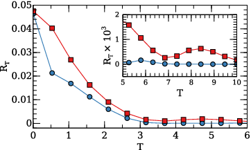
To illustrate the above arguments, we study a chain with spins and , and relate the results of direct numerical simulations to expressions (7), (15), and (19). Although the Ising chain in a transverse field is exactly solvable Pfeuty 1970, we obtain the states and by direct numerical diagonalization of the corresponding Hamiltonians. Next, we use gradient Broyden-Fletcher-Goldfarb-Shanno (BFGS) algorithm Fletcher 1988 in direct numerical search of . Exact numerical diagonalization was used in order to calculate dependent propagators (2). In Fig. 2 we show non-optimized () and optimized infidelities obtained by direct numerical simulations. To quantify linear approximation for the optimized fidelity, we first numerically obtain , , , resulting in as expected, and . It is easy to numerically find a maximum of a function for fixed and ; the example of dependence for is depicted in Fig. 3. From the last line of Table 1 we find and obtain . Additional numerical checks show that adding next harmonic in (5) doesn’t considerably change the optimal fidelity value. Note, that expression (19) being linear in is not linear in since is dependent.
| 0.005 | 0.02 | 0.05 | 0.1 | |
| 648.3 | 162.4 | 65.2 | 32.84 | |
| 0.00322 | 0.0129 | 0.0322 | 0.0642 | |
| 0.644 | 0.644 | 0.643 | 0.642 |

In Fig. 4 (main panel) we show numerically optimized values of , and approximation which follows from expression (14). The coefficient can be obtained by taking product from the first column of Table 1. We see a good agreement between analytical and exact numerical optimization up to . In the inset of Fig. 4 we show numerically optimized values of and see that remains finite in the limit in agreement with (14), and thus our simplification for in (15) was rational. Note, in Fig. 4 we do not have as we used in our analysis. However, the approximation we made is valid because for any finite and .


Important input of (19) is that the optimal control parameters can be evaluated from analysis of function (11), which, in turn, does not contain information about and . Therefore we expect that the optimal control for different quantum Ising chains is only very weakly system-dependent in the ultrashort time limit. This universality is confirmed by Fig. 5 (a) where we present the BFGS optimization results for chains with different parameters.
III.3 Relation to quantum speed limit
The optimal control (14) produces a strong perturbation, where the characteristic energy given by the time-energy uncertainty Mandelstam and Tamm 1991 is proportional to Therefore, it is instructive to consider the quantum speed limit (QSL) time that is the minimal possible time required to transform the initial into the final state Margolus and Levitin 1998. The time is computed as Deffner and Lutz 2013:
| (20) |
and the ratio can be considered as the efficiency of the quantum control (see, e.g., Murphy et al. 2010; Caneva et al. 2009). In Fig. 5(b), where we show dependence of , one can see the ratio , and this relatively large value can be related to the locality of the control.

IV From ultrafast to adiabatic evolution
Here we briefly discuss features of optimal control when the evolution time runs from ultrashort values to the adiabatic domain. In Fig. 6 we show non-optimized and optimized infidelity for an extended interval of As can be seen, the non-optimized infidelity goes to zero as a consequence of adiabaticity (4). Also, the maximal difference between optimized and non-optimized infidelity appears at short time .
As we have shown in Refs. Pyshkin et al. 2018; Pyshkin et al. 2019 the optimal shape of control function is restricted by two requirements: (1) continuous transition from non-adiabatic to adiabatic time domain, and (2) nonzero time derivative at and These two assumptions lead to the following conditions:
| (21) |
written in parametrization (5) as:
| (22) |
Remarkably, the conditions (22) are independent. It turns out that from the numerical calculations satisfies (22) for ultrashort, short, and adiabatic processes, regardless of the time domain (this statement is as well independent when we take more than two harmonics in (5)). Note that first two harmonics in (5) provide the simplest efficient parametrization, which satisfies (21), for a strong energy pumping, with at a finite time interval.
In Fig. 7 we show the landscape of output fidelity as a function of for . One can see that the high-fidelity “islands” form horizontal equidistant lines. Appearance of these lines is related to possibility of the satisfaction of (13) by letting with (see Eqs.(8) and (9)). In comparison with the fidelity of different local maximums we see that initial point is the valid choice for numerical BFGS search in order to avoid traps Rabitz et al. 2004; Ho and Rabitz 2006; Pechen and Tannor 2011; Zhdanov and Seideman 2015; Zhdanov 2018, and our assumption is corroborated. Moreover, the universal initial point (which satisfies (22)) for numerical search connects together adiabatic and non-adiabatic time domains.

V Conclusion
We demonstrated that properly-designed incomplete local control can greatly decrease infidelity of unitary evolution in the non-adiabatic time domain, even for ultrafast transition processes. We presented an approximate analytical solution for finding the optimal control parameters in the ultrashort domain and showed that optimization can lead to a linear in decrease in the infidelity. Rather than achieving zero infidelity, this linearity is the main benefit of using the unrestricted energy resource in the case of incomplete local control.
The main features of the optimal control found by heuristic reasoning and analytical derivations have been confirmed by direct numerical simulations. Our results show that optimal control parameters for short , being system-independent, are somehow universal. Surprisingly, in our approach one needs to only analyze one of extrema of a single-variable analytical function to find the optimal control parameters instead of the conventional numerical algorithm for computing propagators. We hope that our findings and approaches will be useful for further improvements of efficiency in realistic quantum control in broad variety of systems.
Acknowledgements
We gratefully acknowledge National Research, Development and Innovation Office of Hungary (Project Nos. K124351 and 2017-1.2.1-NKP-2017-00001), the Basque Country Government (Grant No. IT472-10), the Spanish Ministry of Economy, Industry, and Competitiveness (MINECO) and the European Regional Development Fund FEDER Grant No. FIS2015-67161-P (MINECO/FEDER, UE).
References
- Peirce et al. (1988) A. P. Peirce, M. A. Dahleh, and H. Rabitz, Phys. Rev. A 37, 4950 (1988).
- Brif et al. (2010) C. Brif, R. Chakrabarti, and H. Rabitz, New Journal of Physics 12, 075008 (2010).
- Borzi et al. (2017) A. Borzi, G. Ciaramella, and M. Sprengel, Formulation and Numerical Solution of Quantum Control Problems (Computational Science & Engineering) (SIAM-Society for Industrial & Applied Mathematics, 2017).
- Caneva et al. (2011a) T. Caneva, T. Calarco, R. Fazio, G. E. Santoro, and S. Montangero, Phys. Rev. A 84, 012312 (2011a).
- Caneva et al. (2014) T. Caneva, A. Silva, R. Fazio, S. Lloyd, T. Calarco, and S. Montangero, Phys. Rev. A 89, 042322 (2014).
- Li et al. (2011) Y. Li, L.-A. Wu, Y.-D. Wang, and L.-P. Yang, Phys. Rev. B 84, 094502 (2011).
- Luchnikov and Filippov (2017) I. A. Luchnikov and S. N. Filippov, Phys. Rev. A 95, 022113 (2017).
- Wu et al. (2004) L.-A. Wu, D. A. Lidar, and S. Schneider, Phys. Rev. A 70, 032322 (2004).
- Pyshkin et al. (2016) P. V. Pyshkin, E. Y. Sherman, D.-W. Luo, J. Q. You, and L.-A. Wu, Phys. Rev. B 94, 134313 (2016).
- Torres et al. (2017) J. M. Torres, J. Z. Bernád, G. Alber, O. Kálmán, and T. Kiss, Phys. Rev. A 95, 023828 (2017).
- Verstraete et al. (2009) F. Verstraete, M. M. Wolf, and J. I. Cirac, Nature Physics 5, 633 (2009).
- Jing and Yu (2010) J. Jing and T. Yu, Phys. Rev. Lett. 105, 240403 (2010).
- Luo et al. (2015) D.-W. Luo, P. V. Pyshkin, C.-H. Lam, T. Yu, H.-Q. Lin, J. Q. You, and L.-A. Wu, Phys. Rev. A 92, 062127 (2015).
- Schmidt et al. (2011) R. Schmidt, A. Negretti, J. Ankerhold, T. Calarco, and J. T. Stockburger, Phys. Rev. Lett. 107, 130404 (2011).
- Born and Fock (1928) M. Born and V. Fock, Zeitschrift für Physik 51, 165 (1928).
- Torrontegui et al. (2013) E. Torrontegui, S. Ibáñez, S. Martínez-Garaot, M. Modugno, A. del Campo, D. Guéry-Odelin, A. Ruschhaupt, X. Chen, and J. G. Muga, in Advances In Atomic, Molecular, and Optical Physics (Elsevier, 2013) p. 117.
- Guéry-Odelin et al. (2019) D. Guéry-Odelin, A. Ruschhaupt, A. Kiely, E. Torrontegui, S. Martínez-Garaot, and J. G. Muga, Rev. Mod. Phys. 91, 045001 (2019).
- Demirplak and Rice (2003) M. Demirplak and S. A. Rice, The Journal of Physical Chemistry A 107, 9937 (2003).
- Berry (2009) M. V. Berry, Journal of Physics A: Mathematical and Theoretical 42, 365303 (2009).
- Ren et al. (2017) F.-H. Ren, Z.-M. Wang, and Y.-J. Gu, Physics Letters A 381, 70 (2017).
- Loss and DiVincenzo (1998) D. Loss and D. P. DiVincenzo, Phys. Rev. A 57, 120 (1998).
- Burkard et al. (1999) G. Burkard, D. Loss, and D. P. DiVincenzo, Phys. Rev. B 59, 2070 (1999).
- Das and Chakrabarti (2008) A. Das and B. K. Chakrabarti, Rev. Mod. Phys. 80, 1061 (2008).
- McGeoch (2014) C. C. McGeoch, Adiabatic Quantum Computation and Quantum Annealing: Theory and Practice (Synthesis Lectures on Quantum Computing) (Morgan & Claypool, 2014).
- Schirmer et al. (2002) S. G. Schirmer, A. I. Solomon, and J. V. Leahy, Journal of Physics A: Mathematical and General 35, 4125 (2002).
- Ramakrishna et al. (1995) V. Ramakrishna, M. V. Salapaka, M. Dahleh, H. Rabitz, and A. Peirce, Phys. Rev. A 51, 960 (1995).
- Burgarth et al. (2009) D. Burgarth, S. Bose, C. Bruder, and V. Giovannetti, Phys. Rev. A 79, 060305(R) (2009).
- Caneva et al. (2011b) T. Caneva, T. Calarco, and S. Montangero, Phys. Rev. A 84, 022326 (2011b).
- Rach et al. (2015) N. Rach, M. M. Müller, T. Calarco, and S. Montangero, Phys. Rev. A 92, 062343 (2015).
- Sakurai and Napolitano (2010) J. J. Sakurai and J. J. Napolitano, Modern Quantum Mechanics (2nd Edition) (Pearson, 2010).
- (31) In other words, we change the real function (which as we assume must have a property ) to a constant . Thus the factor in Eq.(7).
- Pfeuty (1970) P. Pfeuty, Annals of Physics 57, 79 (1970).
- Fletcher (1988) R. Fletcher, Practical Methods of Optimization, 2nd Edition (Wiley, 1988).
- Mandelstam and Tamm (1991) L. Mandelstam and I. Tamm, in Selected Papers, edited by B. M. Bolotovskii, V. Y. Frenkel, and R. Peierls (Springer Berlin Heidelberg, Berlin, Heidelberg, 1991) p. 115.
- Margolus and Levitin (1998) N. Margolus and L. B. Levitin, Physica D: Nonlinear Phenomena 120, 188 (1998).
- Deffner and Lutz (2013) S. Deffner and E. Lutz, Journal of Physics A: Mathematical and Theoretical 46, 335302 (2013).
- Murphy et al. (2010) M. Murphy, S. Montangero, V. Giovannetti, and T. Calarco, Phys. Rev. A 82, 022318 (2010).
- Caneva et al. (2009) T. Caneva, M. Murphy, T. Calarco, R. Fazio, S. Montangero, V. Giovannetti, and G. E. Santoro, Phys. Rev. Lett. 103, 240501 (2009).
- Pyshkin et al. (2018) P. V. Pyshkin, E. Y. Sherman, J. Q. You, and L.-A. Wu, New Journal of Physics 20, 105006 (2018).
- Pyshkin et al. (2019) P. Pyshkin, E. Sherman, and L.-A. Wu, Acta Physica Polonica A 135, 1198 (2019).
- Rabitz et al. (2004) H. A. Rabitz, M. M. Hsieh, and C. M. Rosenthal, Science 303, 1998 (2004).
- Ho and Rabitz (2006) T.-S. Ho and H. Rabitz, Journal of Photochemistry and Photobiology A: Chemistry 180, 226 (2006).
- Pechen and Tannor (2011) A. N. Pechen and D. J. Tannor, Phys. Rev. Lett. 106, 120402 (2011).
- Zhdanov and Seideman (2015) D. V. Zhdanov and T. Seideman, Phys. Rev. A 92, 052109 (2015).
- Zhdanov (2018) D. V. Zhdanov, Journal of Physics A: Mathematical and Theoretical 51, 508001 (2018).